Existence of a weak solution to a nonlinear ﬂuid-structure ...canic/KoiterFSI_ARMA.pdf · The...

ARMA manuscript No.(will be inserted by the editor)

Existence of a weak solution to a nonlinearfluid-structure interaction problem modeling

the flow of an incompressible, viscous fluid in acylinder with deformable walls

BORIS MUHA, SUNCICA CANIC

Abstract

We study a nonlinear, unsteady, moving boundary, fluid-structure interaction(FSI) problem arising in modeling blood flow through elastic and viscoelastic ar-teries. The fluid flow, which is driven by the time-dependent pressure data, is gov-erned by 2D incompressible Navier-Stokes equations, while the elastodynamicsof the cylindrical wall is modeled by the 1D cylindrical Koiter shell model. Twocases are considered: the linearly viscoelastic and the linearly elastic Koiter shell.The fluid and structure are fully coupled (2-way coupling) via the kinematic anddynamic lateral boundary conditions describing continuity of velocity (the no-slipcondition), and balance of contact forces at the fluid-structure interface. We proveexistence of weak solutions to the two FSI problems (the viscoelastic and the elas-tic case) as long as the cylinder radius is greater than zero.

The proof is based on a novel semi-discrete, operator splitting numerical scheme,known as the kinematically coupled scheme, introduced in [32] to numericallysolve the underlying FSI problems. The backbone of the kinematically coupledscheme is the well-known Marchuk-Yanenko scheme, also known as the Lie split-ting scheme. We effectively prove convergence of that numerical scheme to a so-lution of the corresponding FSI problem.

1. Introduction

We study the existence of a weak solution to a nonlinear moving boundary, un-steady, fluid-structure interaction (FSI) problem between an incompressible, vis-cous, Newtonian fluid, flowing through a cylindrical 2D domain, whose lateralboundary is modeled as a cylindrical Koiter shell. See Figure 1. Two Koiter shellmodels are considered: the linearly viscoelastic and the linearly elastic model.

The fluid flow is driven by the time-dependent inlet and outlet dynamic pres-sure data. The fluid and structure are fully coupled via the kinematic and dynamic

2 BORIS MUHA, SUNCICA CANIC

lateral boundary conditions describing continuity of velocity (the no-slip condi-tion), and balance of contact forces at the fluid-structure interface.

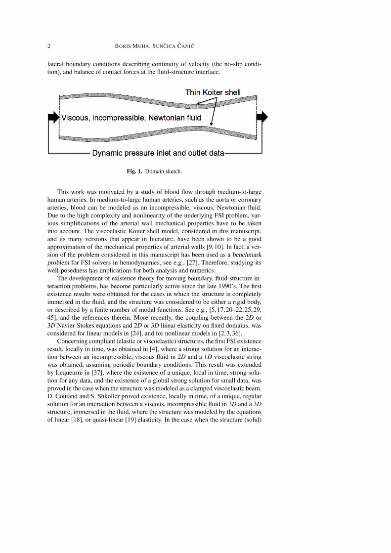
Fig. 1. Domain sketch.

This work was motivated by a study of blood flow through medium-to-largehuman arteries. In medium-to-large human arteries, such as the aorta or coronaryarteries, blood can be modeled as an incompressible, viscous, Newtonian fluid.Due to the high complexity and nonlinearity of the underlying FSI problem, var-ious simplifications of the arterial wall mechanical properties have to be takeninto account. The viscoelastic Koiter shell model, considered in this manuscript,and its many versions that appear in literature, have been shown to be a goodapproximation of the mechanical properties of arterial walls [9,10]. In fact, a ver-sion of the problem considered in this manuscript has been used as a benchmarkproblem for FSI solvers in hemodynamics, see e.g., [27]. Therefore, studying itswell-posedness has implications for both analysis and numerics.

The development of existence theory for moving boundary, fluid-structure in-teraction problems, has become particularly active since the late 1990’s. The firstexistence results were obtained for the cases in which the structure is completelyimmersed in the fluid, and the structure was considered to be either a rigid body,or described by a finite number of modal functions. See e.g., [5,17,20–22,25,29,45], and the references therein. More recently, the coupling between the 2D or3D Navier-Stokes equations and 2D or 3D linear elasticity on fixed domains, wasconsidered for linear models in [24], and for nonlinear models in [2,3,36].

Concerning compliant (elastic or viscoelastic) structures, the first FSI existenceresult, locally in time, was obtained in [4], where a strong solution for an interac-tion between an incompressible, viscous fluid in 2D and a 1D viscoelastic stringwas obtained, assuming periodic boundary conditions. This result was extendedby Lequeurre in [37], where the existence of a unique, local in time, strong solu-tion for any data, and the existence of a global strong solution for small data, wasproved in the case when the structure was modeled as a clamped viscoelastic beam.D. Coutand and S. Shkoller proved existence, locally in time, of a unique, regularsolution for an interaction between a viscous, incompressible fluid in 3D and a 3Dstructure, immersed in the fluid, where the structure was modeled by the equationsof linear [18], or quasi-linear [19] elasticity. In the case when the structure (solid)

Title Suppressed Due to Excessive Length 3

is modeled by a linear wave equation, I. Kukavica and A. Tufahha proved the exis-tence, locally in time, of a strong solution, assuming lower regularity for the initialdata [35]. A fuid-structure interaction between a viscous, incompressible fluid in3D, and 2D elastic shells was considered in [13,12] where existence, locally intime, of the unique regular solution was proved. All the above mentioned exis-tence results for strong solutions are local in time. We also mention that the worksof Shkoller et al., and Kukavica at al. were obtained in the context of Lagrangiancoordinates, which were used for both the structure and fluid problems.

In the context of weak solutions, the following results have been obtained.Continuous dependence of weak solutions on initial data for a fluid structure inter-action problem with a free boundary type coupling condition was studied in [33].Existence of a weak solution for a FSI problem between a 3D incompressible, vis-cous fluid and a 2D viscoelastic plate was considered by Chambolle et al. in [11],while Grandmont improved this result in [31] to hold for a 2D elastic plate. In theseworks existence of a weak solution was proved for as long as the elastic boundarydoes not touch ”the bottom” (rigid) portion of the fluid domain boundary.

In the present manuscript we prove the existence of a weak solution to a FSIproblem modeling the flow of an incompressible, viscous, Newtonian fluid flowingthrough a cylinder whose lateral wall is described by the linearly viscoelastic, orby the linearly elastic Koiter shell equations. The fluid domain is two-dimensional,while the structure equations are in 1D. The two existence results (the viscoelas-tic case and the elastic case) hold for as long as the compliant tube walls do nottouch each other. The main novelty of this work is in the methodology of proof.The proof is based on a semi-discrete, operator splitting Lie scheme, which wasused in [32] for a design of a stable, loosely coupled numerical scheme, called thekinematically coupled scheme (see also [7]). Therefore, in this work, we effec-tively prove that the kinematically coupled scheme converges to a weak solutionof the underlying FSI problem. To the best of our knowledge, this is the first resultof this kind in the area of nonlinear FSI problems. Semi-discretization is a wellknown method for proving existence of weak solutions to the Navier-Stokes equa-tions, see e.g. [47], Ch. III.4. The Lie operator splitting scheme, also known as theMarchuk-Yanenko scheme, has been widely used in numerical computations, see[30] and the references therein. Temam used a combination of these approachesin [46] to prove the existence of a solution of the nonlinear Carleman equation.The present manuscript represents the first use of this methodology in the area ofnonlinear FSI problems. This method is robust in the sense that it can be applied tothe viscoelastic case and to the elastic case, independently. Namely, our existenceresult in the case when the structure is purely elastic in not obtained in the limit,as the regularization provided by structural viscosity tends to zero.

Another novelty of this work is in the the boundary conditions, which are notperiodic, but are motivated by the blood flow application and are given by theprescribed inlet and outlet dynamic pressure data. This means that the Lagrangianframework for the treatment of the entire coupled FSI problem cannot be usedin this context, and so we employed the Arbitrary Langrangian-Eulerian (ALE)method to deal with the motion of the fluid domain.


Our proof is constructive, and its main steps have already been implemented inthe design of several stable computational FSI schemes for the simulation of bloodflow in human arteries [7,26,32,34]. The main steps in the proof include the ALEweak formulation and the time-discretization via Lie operator splitting. Solu-tions to the time-discretized problems define a sequence of approximate solutionsto the continuous time-dependent problem. The time-dependent FSI problem isdiscretized in time in such a way that at each time step, this multi-physics problemis split into two sub-problems: the fluid and the structure sub-problem. However,to achieve stability and convergence of the corresponding numerical scheme [32],the splitting had to be performed in a special way in which the fluid sub-problemincludes structure inertia (and structural viscosity in the viscoelastic case) via a”Robin-type” boundary condition. See [8] for more details. The fact that structureinertia (and structural viscosity) are included implicitly in the fluid sub-problem,enabled us, in the present work, to get appropriate energy estimates for the ap-proximate solutions, independently of the size of time discretization. Passing tothe limit, as the size of the time step converges to zero, is achieved by the use ofcompactness arguments and a careful construction of the appropriate test functionsassociated with moving domains. The main difference between the viscoelasticand the elastic case is in the compactness argument.

The main body of the manuscript is dedicated to the proof in the case whenthe structure is modeled as a linearly viscoelastic Koiter shell. In Section 8 wesummarize the main steps of the proof in the case when the structure is modeledas a linearly elastic Koiter shell.

2. Problem description

We consider the flow of an incompressible, viscous fluid in a two-dimensional,symmetric cylinder (or channel) of reference length L, and reference width 2R, seeFigure 2.

Fig. 2. Domain sketch and notation.

Without loss of generality, we consider only the upper half of the fluid domainsupplemented by a symmetry boundary condition at the bottom boundary. Thus,the reference domain is (0,L)× (0,R) with the lateral (top) boundary given by(0,L)×R.


We will be assuming that the lateral boundary of the cylinder is deformable andthat its location is not known a priori, but is fully coupled to the motion of the vis-cous, incompressible fluid occupying the fluid domain. Furthermore, it will be as-sumed that the lateral boundary is a thin, isotropic, homogeneous structure, whosedynamics is modeled by the cylindrical, linearly viscoelastic, or by the cylindricallinearly elastic Koiter shell equations. Additionally, for simplicity, we will be as-suming that only the displacement in vertical (radial) direction is non-negligible.The (vertical) displacement from the reference configuration will be denoted byη(t,z). See Figure 2. Models of this kind are common in blood flow applications[9,42,44], where the lateral boundary of the cylinder corresponds to arterial walls.

The fluid domain, which depends on time and is not known a priori, will bedenoted by

Ωη(t) = (z,r) ∈ R2 : z ∈ (0,L), r ∈ (0,R+η(t,x),

and the corresponding lateral (top) boundary by

Γη(t) = (z,r) ∈ R2 : r = R+η(t,z), z ∈ (0,L).

The “bottom” (symmetry) boundary of the fluid domain will be denoted by Γb =(0,L)×0, while the inlet and outlet sections of the fluid domain boundary byΓin = 0× (0,R), Γout = L× (0,R). See Figure 2.

The fluid problem: We are interested in studying a dynamic pressure-drivenflow through Ωη(t) of an incompressible, viscous fluid modeled by the Naiver-Stokes equations:

ρ f (∂tu+u ·∇u) = ∇ ·σ ,∇ ·u = 0,

in Ωη(t), t ∈ (0,T ), (1)

where ρ f denotes the fluid density, u fluid velocity, p fluid pressure, σ = −pI+2µD(u) is the Cauchy stress tensor of the fluid, µ is the kinematic viscosity coef-ficient, and D(u) = 1

2 (∇u+∇τ u) is the symmetrized gradient of u.At the inlet and outlet boundaries we prescribe zero tangential velocity and

dynamic pressure p+ ρ f2 |u|

2 (see e.g. [16]):

p+ρ f

2|u|2 = Pin/out(t),

ur = 0,

on Γin/out , (2)

where Pin/out ∈ L2loc(0,∞) are given. Therefore the fluid flow is driven by a pre-

scribed dynamic pressure drop, and the flow enters and leaves the fluid domainorthogonally to the inlet and outlet boundary.

At the bottom boundary we prescribe the symmetry boundary condition:

ur = ∂ruz = 0, on Γb. (3)

The structure problem, namely, the dynamics of the lateral boundary, is de-fined by the linearly viscoelastic cylindrical Koiter shell equations capturing radialdisplacement η (for the purely elastic problem see Section 8):

ρsh∂2t η +C0η−C1∂

2z η +C2∂

4z η +D0∂tη−D1∂t∂

2z η +D2∂t∂

4z η = f . (4)


Here, ρs is the structure density, h is the structure thickness, and f is the forcedensity in the radial (vertical) er direction acting on the structure. The constants Ciand Di > 0 are the material constants describing structural elasticity and viscosity,respectively, which are given in terms of four material parameters: the Young’smodulus of elasticity E, and the Poisson ratio σ , and their viscoelastic couter-partsEv and σv (for a derivation of this model and the exact form of the coefficients,please see Appendix, and [7,9]). The purely elastic case, i.e., Di = 0, i = 0,1,2,will be considered in Section 8.

We consider the dynamics of a clamped Koiter shell with the boundary condi-tions

η(0) = ∂zη(0) = η(L) = ∂zη(L) = 0.

The coupling between the fluid and structure is defined by two sets of bound-ary conditions satisfied at the lateral boundary Γη(t). They are the kinematic anddynamic lateral boundary conditions describing continuity of velocity (the no-slipcondition), and continuity of normal stress, respectively. Written in Lagrangianframework, with z ∈ (0,L), and for t ∈ (0,T ), they read:

– The kinematic condition:

(∂tη(t,z),0) = u(t,z,R+η(t,z)), (5)

– The dynamic condition:

f (t,z) =−J(t,z)(σn)|(t,z,R+η(t,z)) · er. (6)

Here, f = f (t,z) corresponds to the right hand-side of equation (4), and J(t,z)=√1+(∂zη(t,z))2 denotes the Jacobian of the transformation from Eulerian to

Lagrangian coordinates.

System (1)–(6) is supplemented with the following initial conditions:

u(0, .) = u0, η(0, .) = η0, ∂tη(0, .) = v0. (7)

Additionally, we will be assuming that the initial data satisfies the followingcompatibility conditions:

u0(z,R+η0(z)) = v0(z)er, z ∈ (0,L),η0(0) = η0(L) = v0(0) = v0(L) = 0,

R+η0(z)> 0, z ∈ [0,L].(8)

Notice that the last condition requires that the initial displacement is such that thelateral boundary does not touch the bottom of the domain. This is an importantcondition which will be used at several places throughout this manuscript.

In summary, we study the following fluid-structure interaction problem:

Problem 1. Find u = (uz(t,z,r),ur(t,z,r)), p(t,z,r), and η(t,z) such that


ρ f(∂tu+(u ·∇)u

)= ∇ ·σ

∇ ·u = 0

in Ωη(t), t ∈ (0,T ), (9)

u = ∂tηer,ρsh∂ 2

t η +C0η−C1∂ 2z η +C2∂ 4

z η

+D0∂tη−D1∂t∂2z η +D2∂t∂

4z η = −Jσn · er,

on (0,T )× (0,L), (10)

ur = 0,∂ruz = 0,

on (0,T )×Γb, (11)

p+ ρ f2 |u|

2 = Pin/out(t),ur = 0,

on (0,T )×Γin/out , (12)

u(0, .) = u0,η(0, .) = η0,

∂tη(0, .) = v0.

at t = 0. (13)

This is a nonlinear, moving-boundary problem, which captures the full, two-way fluid-structure interaction coupling. The nonlinearity in the problem is repre-sented by the quadratic term in the fluid equations, and by the nonlinear couplingbetween the fluid and structure defined at the lateral boundary Γη(t), which is oneof the unknowns in the problem.

2.1. The energy of the problem

Problem (1) satisfies the following energy inequality:

ddt

E(t)+D(t)≤C(Pin(t),Pout(t)), (14)

where E(t) denotes the sum of the kinetic energy of the fluid and of the structure,and the elastic energy of the Koiter shell:

E(t) =ρ f

2‖u‖2

L2(Ωη (t))+

ρsh2‖∂tη‖2

L2(0,L)

+12(C0‖η‖2

L2(0,L)+C1‖∂zη‖2L2(0,L)+C2‖∂ 2

z η‖2L2(0,L)

),

(15)

the term D(t) captures dissipation due to structural and fluid viscosity:

D(t)= µ‖D(u)‖2L2(Ωη (t)))

+D0‖∂tη‖2L2(0,L)+D1‖∂t∂zη‖2

L2(0,L)+D2‖∂t∂2z η‖2

L2(0,L),

(16)and C(Pin(t),Pout(t))) is a constant which depends only on the inlet and outletpressure data, which are both functions of time.

To show that (14) holds, we first multiply equation (1) by u, integrate overΩη(t), and formally integrate by parts to obtain:∫

Ωη (t)ρ f(∂tu ·u+(u ·∇)u ·u

)+2µ

∫Ωη (t)

|Du|2−∫

∂Ωη (t)(−pI+2µD(u))n(t)·u= 0.


To deal with the inertia term we first recall that Ωη(t) is moving in time and that thevelocity of the lateral boundary is given by u|Γ (t). The transport theorem appliedto the first term on the left hand-side of the above equation then gives:∫

Ωη (t)∂tu ·u =

12

ddt

∫Ωη (t)

|u|2− 12

∫Γη (t)|u|2u ·n(t).

The second term on the left hand side can can be rewritten by using integration byparts, and the divergence-free condition, to obtain:∫

Ωη (t)(u ·∇)u ·u =

12

∫∂Ωη (t)

|u|2u ·n(t) = 12(∫

Γη (t)|u|2u ·n(t)

−∫

Γin

|u|2uz +∫

Γout

|u|2uz.)

These two terms added together give∫Ωη (t)

∂tu ·u+∫

Ωη (t)(u ·∇)u ·u =

12

ddt

∫Ωη (t)

|u|2− 12

∫Γin

|u|2uz +12

∫Γout

|u|2uz.

(17)To deal with the boundary integral over ∂Ωη(t), we first notice that on Γin/out

the boundary condition (2) implies ur = 0. Combined with the divergence-freecondition we obtain ∂zuz = −∂rur = 0. Now, using the fact that the normal toΓin/out is n = (∓1,0) we get:∫

Γin/out

(−pI+2µD(u))n ·u =∫

Γin

Pinuz−∫

Γout

Poutuz. (18)

In a similar way, using the symmetry boundary conditions (3), we get:∫Γb

(−pI+2µD(u))n ·u = 0.

What is left is to calculate the remaining boundary integral over Γη(t). For thiswe consider the Koiter shell equation (4), multiply it by ∂tη , and integrate by partsto obtain ∫ L

0f ∂tη =

ρsh2

ddt‖∂tη‖2

L2(0,L)

+12

ddt

(C0‖η‖2

L2(0,L)+C1‖∂zη‖2L2(0,L)+C2‖∂ 2

z η‖2L2(0,L)

)(19)

+D0‖∂tη‖2L2(0,L)+D1‖∂t∂zη‖2

L2(0,L)+D2‖∂t∂2z η‖2

L2(0,L).

By enforcing the dynamic coupling condition (6) we obtain

−∫

Γη (t)σn(t) ·u =−

∫ L

0Jσn ·u =

∫ L

0f ∂tη . (20)


Finally, by combining (20) with (19), and by adding the remaining contribu-tions to the energy of the FSI problem calculated in equations (17) and (18), oneobtains the following energy equality:

ρ f

2ddt

∫Ωη (t)

|u|2 + ρsh2

ddt‖∂tη‖2

L2(0,L)+2µ

∫Ωη (t)

|Du|2 + 12

ddt

(C0‖η‖2

L2(0,L)

+C1‖∂zη‖2L2(0,L)+C2‖∂ 2

z η‖2L2(0,L)

)+D0‖∂tη‖2

L2(0,L) (21)

+D1‖∂t∂zη‖2L2(0,L)+D2‖∂t∂

2z η‖2

L2(0,L) =±Pin/out(t)∫

Σin/out

uz.

By using the trace inequality and Korn inequality one can estimate:

|Pin/out(t)∫

Σin/out

uz| ≤C|Pin/out |‖u‖H1(Ωη (t)) ≤C2ε|Pin/out |2 +

εC2‖D(u)‖2

L2(Ωη (t).

By choosing ε such that εC2 ≤ µ we get the energy inequality (14).

3. The ALE formulation and Lie splitting

3.1. First order ALE formulation

To prove the existence of a weak solution to Problem 1 it is convenient tomap Problem 1 onto a fixed domain Ω . In our approach we choose Ω to be thereference domain Ω = (0,L)×(0,1). We follow the approach typical of numericalmethods for fluid-structure interaction problems and map our fluid domain Ω(t)onto Ω by using an Arbitrary Lagrangian-Eulerian (ALE) mapping [7,32,23,43,44]. We remark here that in our problem it is not convenient to use the Lagrangianformulation of the fluid sub-problem, as is done in e.g., [19,13,35], since, in ourproblem, the fluid domain consists of a fixed, control volume of a cylinder, whichdoes not follow Largangian flow.

We begin by defining a family of ALE mappings Aη parameterized by η :

Aη(t) : Ω →Ωη(t), Aη(t)(z, r) :=(

z(R+η(t, z))r

), (z, r) ∈Ω , (22)

where (z, r) denote the coordinates in the reference domain Ω = (0,L)× (0,1).Mapping Aη(t) is a bijection, and its Jacobian is given by

|det∇Aη(t)|= |R+η(t, z)|. (23)

Composite functions with the ALE mapping will be denoted by

uη(t, .) = u(t, .)Aη(t) and pη(t, .) = p(t, .)Aη(t).

The derivatives of composite functions satisfy:

∂tu = ∂tuη − (wη ·∇η)uη , ∇u = ∇η uη ,


where the ALE domain velocity, wη , and the transformed gradient, ∇η , are givenby:

wη = ∂tη rer, ∇η =

∂z− r∂zη

R+η∂r

1R+η

∂r

. (24)

Note that

∇η v = ∇v(∇Aη)

−1. (25)

The following notation will also be useful:

ση =−pη I+2µDη(uη), Dη(uη) =

12(∇η uη +(∇η)τ uη).

We are now ready to rewrite Problem 1 in the ALE formulation. However, beforewe do that, we will make one more important step in our strategy to prove the exis-tence of a weak solution to Problem 1. Namely, as mentioned in the Introduction,we would like to “solve” the coupled FSI problem by approximating the problemusing time-discretization via operator splitting, and then prove that the solution tothe semi-discrete problem converges to a weak solution of the continuous prob-lem, as the time-discretization step tends to zero. To perform time discretizationvia operator splitting, which will be described in the next section, we need to writeour FSI problem as a first-order system in time. This will be done by replacingthe second-order time-derivative of η , with the first-order time-derivative of thestructure velocity. To do this, we further notice that in the coupled FSI problem,the kinematic coupling condition (5) implies that the structure velocity is equalto the normal trace of the fluid velocity on Γη(t). Thus, we will introduce a newvariable, v, to denote this trace, and will replace ∂tη by v everywhere in the struc-ture equation. This has deep consequences both for the existence proof presentedin this manuscript, as well as for the proof of stability of the underlying numericalscheme, presented in [8], as it enforces the kinematic coupling condition implicitlyin all the steps of the scheme.

Thus, Problem 1 can be reformulated in the ALE framework, on the referencedomain Ω , and written as a first-order system in time, in the following way:

Problem 2. Find u(t, z, r), p(t, z, r),η(t, z), and v(t, z) such that

ρ f(∂tu+((u−wη) ·∇η)u

)= ∇η ·ση ,

∇η ·u = 0,

in (0,T )×Ω , (26)

ur = 0,∂ruz = 0

on (0,T )×Γb, (27)

p+ ρ f2 |u|

2 = Pin/out(t),ur = 0,

on (0,T )×Γin/out , (28)


u = ver,∂tη = v,

ρsh∂tv+C0η−C1∂ 2z η +C2∂ 4

z η

+D0v−D1∂ 2z v+D2∂ 4

z v = −Jσn · er

on (0,T )× (0,L), (29)

u(0, .) = u0,η(0, .) = η0,v(0, .) = v0, at t = 0. (30)

Here, we have dropped the superscript η in uη for easier reading.We are now ready to define the time discretization by operator splitting. The

underlying multi-physics problem will be split into the fluid and structure sub-problems, following the different “physics” in the problem, but the splitting will beperformed in a particularly careful manner, so that the resulting problem definesa scheme which converges to a weak solution of the continuous problem (andprovides a numerical scheme which is unconditionally stable).

3.2. The operator splitting scheme

We use the Lie splitting, also known as the Marchuk-Yanenko splitting scheme.The splitting can be summarized as follows. Let N ∈ N, ∆ t = T/N and tn = n∆ t.Consider the following initial-value problem:

dφ

dt+Aφ = 0 in (0,T ), φ(0) = φ0,

where A is an operator defined on a Hilbert space, and A can be written as A =

A1 +A2. Set φ 0 = φ0, and, for n = 0, . . . ,N − 1 and i = 1,2, compute φ n+ i2 by

solvingddt

φi +Aiφi = 0

φi(tn) = φ n+ i−12

in (tn, tn+1),

and then set φ n+ i2 = φi(tn+1), for i = 1,2. It can be shown that this method is

first-order accurate in time, see e.g., [30].We apply this approach to split Problem 2 in the fluid and structure sub-

problems. During this procedure the structure equation (29) will be split into theviscous part, i.e., the part involving the normal trace of the fluid velocity on Γη(t),v, and the purely elastic part. The viscous part of the structure problem will beused as a boundary condition for the fluid sub-problem, while the elastic part ofthe structure problem will be solved separately. More precisely, we define the split-ting of Problem 2 in the following way:

Problem A1: The structure elastodynamics problem. In this step we solvethe elastodynamics problem for the location of the deformable boundary by involv-ing only the elastic energy of the structure. The motion of the structure is drivenby the initial velocity, which is equal to the trace of the fluid velocity on the lateralboundary, taken from the previous step. The fluid velocity u remains unchanged in


this step. More precisely, the problem reads: Given (un,ηn,vn) from the previoustime step, find (u,v,η) such that:

∂tu = 0, in (tn, tn+1)×Ω ,

ρsh∂tv+C0η−C1∂ 2z η +C2∂ 4

z η = 0 on (tn, tn+1)× (0,L),

∂tη = v on (tn, tn+1)× (0,L),

η(0) = ∂zη(0) = η(L) = ∂zη(L) = 0,

u(tn) = un, η(tn) = ηn, v(tn) = vn.

(31)

Then set un+ 12 = u(tn+1), ηn+ 1

2 = η(tn+1), vn+ 12 = v(tn+1).

Problem A2: The fluid problem. In this step we solve the Navier-Stokesequations coupled with structure inertia and viscoelastic energy of the structure,through a “Robin-type” boundary condition on Γ . The kinematic coupling condi-tion is implicitly satisfied. The structure displacement remains unchanged. With aslight abuse of notation, the problem can be written as follows: Find (u,v,η) suchthat:

∂tη = 0 on (tn, tn+1)× (0,L),

ρ f(∂tu+((un−wη

n+ 12 ) ·∇ηn

)u)= ∇ηn ·σηn

∇ηn ·u = 0

in (tn, tn+1)×Ω ,

ρsh∂tv+D0v−D1∂ 2z v+D2∂ 4

z v = −Jσn · eru = ver

on (tn, tn+1)× (0,L),

ur = 0∂ruz = 0

on (tn, tn+1)×Γb,

p+ ρ f2 |u|

2 = Pin/out(t)ur = 0

on (tn, tn+1)×Γin/out ,

with u(tn, .) = un+ 12 , η(tn, .) = η

n+ 12 , v(tn, .) = vn+ 1

2 . (32)

Then set un+1 = u(tn+1), ηn+1 = η(tn+1), vn+1 = v(tn+1).

Notice that, since in this step η does not change, this problem is linear. Fur-thermore, it can be viewed as a stationary Navier-Stokes-like problem on a fixeddomain, coupled with the viscoelastic part of the structure equation through aRobin-type boundary condition. In numerical simulations, one can use the ALEtransformation Aηn to “transform” the problem back to domain Ωηn and solve itthere, thereby avoiding the un-necessary calculation of the transformed gradient∇ηn

. The ALE velocity is the only extra term that needs to be included with thatapproach. See, e.g., [7] for more details. For the purposes of our proof, we will,however, remain in the fixed, reference domain Ω .


It is important to notice that in Problem A2, the problem is “linearized” aroundthe previous location of the boundary, i.e., we work with the domain determinedby ηn, and not by ηn+1/2. This is in direct relation with the implementation ofthe numerical scheme studied in [7,8]. However, we also notice that ALE velocity,wn+ 1

2 , is taken from the just calculated Problem A1! This choice is crucial forobtaining a semi-discrete version of an energy inequality, discussed in Section 5.

In the remainder of this paper we use the splitting scheme described above todefine approximate solutions of Problem 2 (or equivalently Problem 1) and showthat the approximate solutions converge to a weak solution, as ∆ t→ 0.

4. Weak solutions

4.1. Notation and function spaces

To define weak solutions of the moving-bounday problem 2 we first introducesome notation which will simplify the subsequent analysis. We begin by introduc-ing the following bilinear forms associated with the elastic and viscoelastic energyof the Koiter shell:

aS(η ,ψ) =∫ L

0

(C0ηψ +C1∂zη∂zψ +C2∂

2z η∂

2z ψ), (33)

a′S(η ,ψ) =∫ L

0

(D0ηψ +D1∂zη∂zψ +D2∂

2z η∂

2z ψ). (34)

Furthermore, we will be using b to denote the following trilinear form correspond-ing to the (symmetrized) nonlinear term in the Navier-Stokes equations:

b(t,u,v,w) =12

∫Ωη (t)

(u ·∇)v ·w− 12

∫Ωη (t)

(u ·∇)w ·v. (35)

Finally, we define a linear functional which associates the inlet and outlet dynamicpressure boundary data to a test function v in the following way:

〈F(t),v〉Γin/out = Pin(t)∫

Γin

vz−Pout(t)∫

Γout

vz.

To define a weak solution to Problem 2 we introduce the necessary functionspaces. For the fluid velocity we will need the classical function space

VF(t) = u = (uz,ur) ∈ H1(Ωη(t))2 : ∇ ·u = 0,uz = 0 on Γ (t), ur = 0 on ∂Ωη(t)\Γ (t). (36)

The function space associated with weak solutions of the Koiter shell is given by

VS = H20 (0,L). (37)

Motivated by the energy inequality we also define the corresponding evolutionspaces for the fluid and structure sub-problems, respectively:

WF(0,T ) = L∞(0,T ;L2(Ωη(t))∩L2(0,T ;VF(t)) (38)


WS(0,T ) =W 1,∞(0,T ;L2(0,L))∩H1(0,T ;VS). (39)

The solution space for the coupled fluid-structure interaction problem must involvethe kinematic coupling condition. Thus, we define

W (0,T ) = (u,η) ∈WF(0,T )×WS(0,T ) : u(t,z,R+η(t,z)) = ∂tη(t,z)er.(40)

The corresponding test space will be denoted by

Q(0,T ) = (q,ψ) ∈C1c ([0,T );VF ×VS) : q(t,z,R+η(t,z)) = ψ(t,z)er. (41)

4.2. Weak solution on the moving domain

We are now in a position to define weak solutions of our moving-boundaryproblem, defined on the moving domain Ωη(t).

Definition 1. We say that (u,η) ∈W (0,T ) is a weak solution of Problem 1 if forevery (q,ψ) ∈Q(0,T ) the following equality holds:

ρ f(−∫ T

0

∫Ωη (t)

u ·∂tq+∫ T

0b(t,u,u,q)

)+2µ

∫ T

0

∫Ωη (t)

D(u) : D(q)

−ρ f

2

∫ T

0

∫ L

0(∂tη)2

ψ−ρsh∫ T

0

∫ L

0∂tη∂tψ +

∫ T

0

(aS(η ,ψ)+a′S(∂tη ,ψ)

)=∫ T

0〈F(t),q〉Γin/out +ρ f

∫Ωη0

u0 ·q(0)+ρsh∫ L

0v0ψ(0).

(42)

In deriving the weak formulation we used integration by parts in a classicalway, and the following equalities which hold for smooth functions:∫

Ωη (t)(u ·∇)u ·q =

12

∫Ωη (t)

(u ·∇)u ·q− 12

∫Ωη (t)

(u ·∇)q ·u

+12

∫ L

0(∂tη)2

ψ± 12

∫Γout/in

|ur|2vr,

∫ T

0

∫Ωη (t)

∂tu ·q =−∫ T

0

∫Ωη (t)

u ·∂tq−∫

Ωη0

u0 ·q(0)−∫ T

0

∫ L

0(∂tη)2

ψ.

4.3. Weak solution on a fixed, reference domain

Since most of our analysis will be performed on the problem defined on thefixed, reference domain Ω , we rewrite the above definition in terms of Ω using theALE mapping Aη(t) defined in (22). For this purpose, we introduce the notation forthe transformed trilinear functional bη , and the function spaces for the composit,transformed functions defined on the fixed domain Ω .

The transformed trilinear form bη is defined as:

bη(u,u,q) =12

∫Ω

(R+η)(((u−wη) ·∇η)u ·q− ((u−wη) ·∇η)q ·u

), (43)


where R+η is the Jacobian of the ALE mapping, calculated in (23). Notice thatwe have included the ALE domain velocity wη into bη .

It is important to point out that the transformed fluid velocity uη is not divergence-free anymore. Rather, it satisfies the transformed divergence-free condition ∇η ·uη = 0. Therefore we need to redefine the function spaces for the fluid velocity byintroducing

V η

F = u = (uz,ur) ∈ H1(Ω)2 : ∇η ·u = 0, uz = 0 on Γ , ur = 0 on ∂Ω \Γ .

The function spaces W η

F (0,T ) and W η(0,T ) are defined the same as before, butwith V η

F instead VF(t). More precisely:

W η

F (0,T ) = L∞(0,T ;L2(Ω)∩L2(0,T ;V η

F (t)), (44)

W η(0,T ) = (u,η) ∈W η

F (0,T )×WS(0,T ) : u(t,z,1) = ∂tη(t,z)er. (45)

The corresponding test space is defined by

Qη(0,T ) = (q,ψ) ∈C1c ([0,T );V

η

F ×VS) : q(t,z,1) = ψ(t,z)er. (46)

Definition 2. We say that (u,η) ∈W η(0,T ) is a weak solution of Problem 2 de-fined on the reference domain Ω , if for every (q,ψ) ∈ Qη(0,T ) the followingequality holds:

ρ f(−∫ T

0

∫Ω

(R+η)u ·∂tq+∫ T

0bη(u,u,q)

)+2µ

∫ T

0

∫Ω

(R+η)Dη(u) : Dη(q)−ρ f

2

∫ T

0

∫Ω

(∂tη)u ·q

−ρsh∫ T

0

∫ L

0∂tη∂tψ +

∫ T

0

(aS(η ,ψ)+a′S(∂tη ,ψ)

)= R

∫ T

0

(Pin(t)

∫ 1

0(qz)|z=0−Pout(t)

∫ 1

0(qz)|z=L

)+ρ f

∫Ωη0

u0 ·q(0)+ρsh∫ L

0v0ψ(0).

(47)

To see that this is consistent with the weak solution defined in Definition 1,we present the main steps in the transformation of the first integral on the lefthand-side in (42), responsible for the fluid kinetic energy. Namely, we formallycalculate:

−∫

Ωη

u ·∂tq =−∫

Ω

(R+η)uη · (∂tq− (wη ·∇η)q) =−∫

Ω

(R+η)uη ·∂tq

+12

∫Ω

(R+η)(wη ·∇η)q ·uη +12

∫Ω

(R+η)(wη ·∇η)q ·uη .


In the last integral on the right hand-side we use the definition of wη and of ∇η ,given in (24), to obtain∫

Ω

(R+η)(wη ·∇η)q ·uη =∫

Ω

∂tη r ∂rq ·uη .

Using integration by parts with respect to r, keeping in mind that η does not de-pend on r, we obtain

−∫

Ωη

u ·∂tq =−∫

Ω

(R+η)uη · (∂tq− (wη ·∇η)q) =−∫

Ω

(R+η)uη ·∂tq

+12

∫Ω

(R+η)(wη ·∇η)q·uη− 12

∫Ω

(R+η)(wη ·∇η)uη ·q− 12

∫Ω

∂tηuη ·q+ 12

∫ L

0(∂tη)2

ψ,

By using this identity in (42), and by recalling the definitions for b and bη , weobtain exactly the weak form (47).

In the remainder of this manuscript we will be working on the fluid-structureinteraction problem defined on the fixed domain Ω , satisfying the weak formula-tion presented in Definition 2. For brevity of notation, since no confusion is pos-sible, we omit the superscript “tilde” which is used to denote the coordinates ofpoints in Ω .

5. Approximate solutions

In this section we use the Lie operator splitting scheme and semi-discretizationto define a sequence of approximations of a weak solution to Problem 2. Eachof the sub-problems defined by the Lie splitting in Section 3.2 (Problem A1 andProblem A2), will be discretized in time using the Backward Euler scheme. Thisapproach defines a time step, which will be denoted by ∆ t, and a number of timesub-intervals N ∈ N, so that

(0,T ) = ∪N−1n=0 (t

n, tn+1), tn = n∆ t, n = 0, ...,N−1.

For every subdivision containing N ∈ N sub-intervals, we recursively define thevector of unknown approximate solutions

Xn+ i2

N =

un+ i2

N

vn+ i

2N

ηn+ i

2N

,n = 0,1, . . . ,N−1, i = 1,2, (48)

where i = 1,2 denotes the solution of sub-problem A1 or A2, respectively. Theinitial condition will be denoted by

X0 =

u0v0η0

.


The semi-discretization and the splitting of the problem will be performed insuch a way that the discrete version of the energy inequality (14) is preserved atevery time step. This is a crucial ingredient for the existence proof.

We define the semi-discrete versions of the kinetic and elastic energy, origi-nally defined in (15), and of dissipation, originally defined in (16), by the follow-ing:

En+ i

2N =

12

(ρ f

∫Ω

(R+ηn−1+i)|un+ i

2N |2 +ρsh‖v

n+ i2

N ‖2L2(0,L)

+C0‖ηn+ i

2N ‖2

L2(0,L)+C1‖∂zηn+ i

2N ‖2

L2(0,L)+C2‖∂ 2z η

n+ i2

N ‖2L2(0,L)

),

(49)

Dn+1N = ∆ t

(µ

∫Ω

(R+ηn)|Dηn

(un+1N )|2 +D0‖vn+1

N ‖2L2(0,L)+D1‖∂zvn+1

N ‖2L2(0,L)

+D2‖∂ 2z vn+1

N ‖2L2(0,L)

), n = 0, . . . ,N−1, i = 0,1.

(50)Throughout the rest of this section, we fix the time step ∆ t, i.e., we keep N ∈ Nfixed, and study the semi-discretized sub-problems defined by the Lie splitting.To simplify notation, we will omit the subscript N and write (un+ i

2 ,vn+ i2 ,ηn+ i

2 )

instead of (un+ i2

N ,vn+ i

2N ,η

n+ i2

N ).

5.1. Semi-discretization of Problem A1

We write a semi-discrete version of Problem A1 (Structure Elastodynamics),defined by the Lie splitting in (31). In this step u does not change, and so

un+ 12 = un.

We define (vn+ 12 ,ηn+ 1

2 ) ∈H20 (0,L)×H2

0 (0,L) as a solution of the following prob-lem, written in weak form:∫ L

0

ηn+ 12 −ηn

∆ tφ =

∫ L

0vn+ 1

2 φ , φ ∈ L2(0,L),

ρsh∫ L

0

vn+ 12 − vn

∆ tψ +aS(η

n+ 12 ,ψ) = 0, ψ ∈ H2

0 (0,L).

(51)

The first equation is a weak form of the semi-discretized kinematic coupling condi-tion, while the second equation corresponds to a weak form of the semi-discretizedelastodynamics equation.

Proposition 1. For each fixed ∆ t > 0, problem (51) has a unique solution (vn+ 12 ,ηn+ 1

2 )∈H2

0 (0,L)×H20 (0,L).

Proof. The proof is a direct consequence of the Lax-Milgram Lemma applied tothe weak form∫ L

0η

n+ 12 ψ +(∆ t)2aS(η

n+ 12 ,ψ) =

∫ L

0

(∆ tvn +η

n)ψ, ψ ∈ H2

0 (0,L),


which is obtained after elimination of vn+ 12 in the second equation, by using the

kinematic coupling condition given by the first equation. ut

Proposition 2. For each fixed ∆ t > 0, solution of problem (51) satisfies the follow-ing discrete energy equality:

En+ 1

2N +

12(ρsh‖vn+ 1

2 − vn‖2 +C0‖ηn+ 12 −η

n‖2

+C1‖∂z(ηn+ 1

2 −ηn)‖2 +C2‖∂ 2

z (ηn+ 1

2 −ηn)‖2)= En

N ,(52)

where the kinetic energy EnN is defined in (49).

Proof. From the first equation in (51) we immediately get

vn+ 12 =

ηn+ 12 −ηn

∆ t∈ H2

0 (0,L).

Therefore we can take vn+ 12 as a test function in the second equation in (51). We

replace the test function ψ by vn+ 12 in the first term on the left hand-side, and

replace ψ by (ηn+ 12 −ηn)/∆ t in the bilinear form aS. We then use the algebraic

identity (a− b) · a = 12 (|a|

2 + |a− b|2 − |b|2) to deal with the terms (vn+1/2 −vn)vn+1/2 and (ηn+1/2−ηn)ηn+1/2. After multiplying the entire equation by ∆ t,the second equation in (51) can be written as:

ρsh(‖vn+ 12 ‖2 +‖vn+ 1

2 − vn‖2)+aS(ηn+ 1

2 ,ηn+ 12 )+aS(η

n+ 12 −η

n,ηn+ 12 −η

n)

= ρsh‖vn‖2 +aS(ηn,ηn).

We then recall that un+ 12 = un in this sub-problem, and so we can add ρ f

∫Ω(1+

ηn)un+1/2 on the left hand-side, and ρ f∫

Ω(1+ηn)un on the right hand-side of the

equation, to obtain exactly the energy equality (52). ut

5.2. Semi-discretization of Problem A2

We write a semi-discrete version of Problem A2 (The Fluid Problem), definedby the Lie splitting in (32). In this step η does not change, and so

ηn+1 = η

n+ 12 .

Define (un+1,vn+1) ∈ V ηn

F ×H20 (0,L) by requiring that for each (q,ψ) ∈ V ηn

F ×H2

0 (0,L) such that q|Γ = ψer, the following weak formulation of problem (32)


holds:

ρ f

∫Ω

(R+ηn)

(un+1−un+ 1

2

∆ t·q+

12

[(un− vn+ 1

2 rer) ·∇ηn]

un+1 ·q

−12

[(un− vn+ 1

2 rer) ·∇ηn]

q ·un+1)+

ρ f

2

∫Ω

vn+ 12 un+1 ·q

+2µ∫

Ω(R+ηn)Dηn

(u) : Dηn(q)

+ρsh∫ L

0

vn+1− vn+ 12

∆ tψ +a′S(v

n+1,ψ) = R(Pn

in

∫ 1

0(qz)|z=0−Pn

out

∫ 1

0(qz)|z=L

),

with ∇ηn ·un+1 = 0, un+1|Γ = vn+1er,

(53)

where Pnin/out =

1∆ t

∫ (n+1)∆ t

n∆ tPin/out(t)dt.

Proposition 3. Let ∆ t > 0, and assume that ηn are such that R+ηn ≥ Rmin >0,n = 0, ...,N. Then, the fluid sub-problem defined by (53) has a unique weak so-lution (un+1,vn+1) ∈ V ηn

F ×H20 (0,L).

Proof. The proof is again a consequence of the Lax-Milgram Lemma. More pre-cisely, donote by U the Hilbert space

U = (u,v) ∈ V ηn

F ×H20 (0,L) : u|Γ = vez, (54)

and define the bilinear form associated with problem (53):

a((u,v),(q,ψ)) := ρ f

∫Ω

(R+ηn)

(u ·q+

∆ t2

[(un− vn+ 1

2 rer) ·∇ηn]

u ·q

− ∆ t2

[(un− vn+ 1

2 rer) ·∇ηn]

q ·u)

+ ∆ tρ f

2

∫Ω

vn+ 12 u ·q+∆ t2µ

∫Ω

(R+ηn)Dηn

(u) : Dηn(q)

+ ρsh∫ L

0vψ +∆ ta′S(v,ψ), (u,v),(q,ψ) ∈U .

We need to prove that this bilinear form a is coercive and continuous on U . To seethat a is coercive, we write

a((u,v),(u,v)) = ρ f

∫Ω

(R+ηn +

∆ t2

vn+ 12 )|u|2 +ρsh

∫ L

0v2

+∆ t(2µ

∫Ω

(R+ηn)|Dηn

(u)|2 +a′S(v,v)).

Coercivity follows immediately after recalling that ηn are such that R + ηn ≥Rmin > 0, which implies that R+ηn + ∆ t

2 vn+ 12 = R+ 1

2 (ηn +ηn+ 1

2 )≥ Rmin > 0.


Before we prove continuity notice that from (24) we have:

‖∇ηnu‖L2(Ω) ≤C‖ηn‖H2(0,L)‖u‖H1(Ω).

Therefore, by applying the generalized Holder inequality and the continuous em-bedding of H1 into L4, we obtain

a((u,v),(q,ψ))≤C(

ρ f ‖u‖L2(Ω)‖q‖L2(Ω)+ρsh‖v‖L2(0,L)‖ψ‖L2(0,L)

+∆ t‖ηn‖H2(0,L)(‖un‖H1(Ω)+‖v

n+ 12 ‖H1(0,L))‖u‖H1(Ω)‖q‖H1(Ω)

+ ∆ tµ‖ηn‖2H2(0,L)‖u‖H1(Ω)‖q‖H1(Ω)+∆ t‖v‖H2(0,L)‖ψ‖H2(0,L)

).

This shows that a is continuous. The Lax-Milgram lemma now implies the exis-tence of a unique solution (un+1,vn+1) of problem (53). ut

Proposition 4. For each fixed ∆ t > 0, solution of problem (53) satisfies the follow-ing discrete energy inequality:

En+1N +

ρ f

2

∫Ω

(R+ηn)|un+1−un|2 + ρsh

2‖vn+1− vn+ 1

2 ‖2L2(0,L)

+Dn+1N ≤ E

n+ 12

N +C∆ t((Pnin)

2 +(Pnout)

2),

(55)

where the kinetic energy EnN and dissipation Dn

N are defined in (49) and (50), andthe constant C depends only on the parameters in the problem, and not on ∆ t (orN).

Proof. We begin by focusing on the weak formulation (53) in which we replacethe test functions q by un+1 and ψ by vn+1. We multiply the resulting equation by∆ t, and notice that the first term on the right hand-side is given by

ρ f

2

∫Ω

(R+ηn)|un+1|2.

This is the term that contributes to the discrete kinetic energy at the time step n+1,but it does not have the correct form, since the discrete kinetic energy at n+ 1 isgiven in terms of the structure location at n+1, and not at n, namely, the discretekinetic energy at n+1 involves

ρ f

2

∫Ω

(R+ηn+1)|un+1|2.

To get around this difficulty it is crucial that the advection term is present in thefluid sub-problem. The advection term is responsible for the presence of the inte-gral

ρ f

2

∫Ω

∆ tvn+ 12 |un+1|2

which can be re-written by noticing that ∆ tvn+ 12 := (ηn+1/2−ηn) which is equal

to (ηn+1−ηn) since, in this sub-problem ηn+1 = ηn+1/2. This implies

ρ f

2

(∫Ω

(R+ηn)|un+1|2 +∆ tvn+ 1

2 |un+1|2)=

ρ f

2

∫Ω

(R+ηn+1)|un+1|2.


Thus, these two terms combined provide the discrete kinetic energy at the timestep n+ 1. It is interesting to notice how the nonlinearity of the coupling at thedeformed boundary requires the presence of nonlinear advection in order for thediscrete kinetic energy of the fluid sub-problem to be decreasing in time, and tothus satisfy the desired energy estimate.

To complete the proof one simply uses the algebraic identity (a− b) · a =12 (|a|

2 + |a−b|2−|b|2) in the same way as in the proof of Proposition 2. ut

We pause for a second, and summarize what we have accomplished so far. Fora given ∆ t > 0 we divided the time interval (0,T ) into N = T/∆ t sub-intervals(tn, tn+1),n = 0, ...,N−1. On each sub-interval (tn, tn+1) we “solved” the coupledFSI problem by applying the Lie splitting scheme. First we solved for the structureposition (Problem A1) and then for the fluid flow (Problem A2). We have justshown that each sub-problem has a unique solution, provided that R+ηn ≥ Rmin >0,n = 0, ...,N, and that its solution satisfies an energy estimate. When combined,the two energy estimates provide a discrete version of the energy estimate (14).Thus, for each ∆ t we have a time-marching, splitting scheme which defines anapproximate solution on (0,T ) of our main FSI problem defined in Problem 2, andis such that for each ∆ t the approximate FSI solution satisfies a discrete version ofthe energy estimate for the continuous problem.

What we would like to ultimately show is that, as ∆ t → 0, the sequence ofsolutions parameterized by N (or ∆ t), converges to a weak solution of Problem 2.Furthermore, we also need to show that R+ηn ≥ Rmin > 0 is satisfied for eachn = 0, ...,N−1. In order to obtain this result, it is crucial to show that the discreteenergy of the approximate FSI solutions defined for each ∆ t, is uniformly bounded,independently of ∆ t (or N). This result is obtained by the following Lemma.

Lemma 1. (The uniform energy estimates) Let ∆ t > 0 and N = T/∆ t > 0. Fur-

thermore, let En+ 1

2N ,En+1

N , and D jN be the kinetic energy and dissipation given by

(49) and (50), respectively.There exists a constant C > 0 independent of ∆ t (and N), which depends only

on the parameters in the problem, on the kinetic energy of the initial data E0,and on the energy norm of the inlet and outlet data ‖Pin/out‖2

L2(0,T ), such that thefollowing estimates hold:

1. En+ 1

2N ≤C,En+1

N ≤C, for all n = 0, ...,N−1,2. ∑

Nj=1 D j

N ≤C,

3.N−1

∑n=0

(∫Ω

(R+ηn)|un+1−un|2 +‖vn+1− vn+ 1

2 ‖2L2(0,L)

+‖vn+ 12 − vn‖2

L2(0,L)

)≤C,

4.N−1

∑n=0

((C0‖ηn+1−η

n‖2L2(0,L)+C1‖∂z(η

n+1−ηn)‖2

L2(0,L)

+C2‖∂ 2z (η

n+1−ηn)‖2L2(0,L)

)≤C.


In fact, C = E0 + C(‖Pin‖2

L2(0,T )+‖Pout‖2L2(0,T )

), where C is the constant from

(55), which depends only on the parameters in the problem.

Proof. We begin by adding the energy estimates (52) and (55) to obtain

En+1N +Dn+1

N +12

(ρ f

∫Ω

(R+ηn)|un+1−un|2 +ρsh‖vn+1− vn+ 1

2 ‖2L2(0,L)+

+ρsh‖vn+ 12 − vn‖2

L2(0,L)+C0‖ηn+ 12 −η

n‖2L2(0,L)+C1‖∂z(η

n+ 12 −η

n)‖2L2(0,L)+

+C2‖∂ 2z (η

n+ 12 −η

n)‖2L2(0,L)

)≤ En

N +C∆ t((Pnin)

2 +(Pnout)

2), n = 0, . . . ,N−1.

Then we calculate the sum, on both sides, and cancel the same terms in the kineticenergy that appear on both sides of the inequality to obtain

ENN +

N−1

∑n=0

Dn+1N +

12

N−1

∑n=0

(ρ f

∫Ω

(R+ηn)|un+1−un|2 +ρsh‖vn+1− vn+ 1

2 ‖2L2(0,L)+

+ρsh‖vn+ 12 − vn‖2

L2(0,L)+C0‖ηn+ 12 −η

n‖2L2(0,L)+C1‖∂z(η

n+ 12 −η

n)‖2L2(0,L)+

+C2‖∂ 2z (η

n+ 12 −η

n)‖2L2(0,L)

)≤ E0 +C∆ t

N−1

∑n=0

((Pnin)

2 +(Pnout)

2).

To estimate the term involving the inlet and outlet pressure we recall that on everysub-interval (tn, tn+1) the pressure data is approximated by a constant which isequal to the average value of the pressure over that time interval. Therefore, wehave, after using Holder’s inequality:

∆ tN−1

∑n=0

(Pnin)

2 = ∆ tN−1

∑n=0

(1

∆ t

∫ (n+1)∆ t

n∆ tPin(t)dt

)2

≤ ‖Pin‖2L2(0,T ).

By using the pressure estimate to bound the right hand-side in the above energyestimate, we have obtained all the statements in the Lemma, with the constant Cgiven by C = E0 +C‖Pin/out‖2

L2(0,T ).

Notice that Statement 1 can be obtained in the same way by summing from 0to n−1, for each n, instead of from 0 to N−1. ut

We will use this Lemma in the next section to show convergence of approxi-mate solutions.


Fig. 3. A sketch of uN .

6. Convergence of approximate solutions

We define approximate solutions of Problem 2 on (0,T ) to be the functionswhich are piece-wise constant on each sub-interval ((n−1)∆ t,n∆ t], n = 1 . . .N of(0,T ), such that for t ∈ ((n−1)∆ t,n∆ t], n = 1 . . .N,

uN(t, .) = unN , ηN(t, .) = η

nN , vN(t, .) = vn

N , v∗N(t, .) = vn− 1

2N . (56)

See Figure 3. Notice that functions v∗N = vn−1/2N are determined by Step A1 (the

elastodynamics sub-problem), while functions vN = vnN are determined by Step A2

(the fluid sub-problem). As a consequence, functions vN are equal to the normaltrace of the fluid velocity on Γ , i.e., uN = vNer. This is not necessarily the case forthe functions v∗N . However, we will show later that the difference between the twosequences converges to zero in L2.

Using Lemma 1 we now show that these sequences are uniformly bounded inthe appropriate solution spaces.

We begin by showing that (ηN)N∈N is uniformly bounded in L∞(0,T ;H20 (0,L)),

and that there exists a T > 0 for which R+ηnN > 0 holds independently of N and

n. This implies, among other things, that our approximate solutions are, indeed,well-defined on a non-zero time interval (0,T ).

Proposition 5. Sequence (ηN)N∈N is uniformly bounded in

L∞(0,T ;H20 (0,L)).

Moreover, for T small enough, we have

0 < Rmin ≤ R+ηN(t,z)≤ Rmax, ∀N ∈ N,z ∈ (0,L), t ∈ (0,T ). (57)

Proof. From Lemma 1 we have that EnN ≤C, where C is independent of N. This

implies

‖ηN(t)‖2L2(0,L),‖∂zηN(t)‖2

L2(0,L),‖∂2zzηN(t)‖2

L2(0,L) ≤C, ∀t ∈ [0,T ].


Therefore,‖ηN‖L∞(0,T ;H2

0 (0,L))≤C.

To show that the radius R+ηN is uniformly bounded away from zero for T smallenough, we first notice that the above inequality implies

‖ηnN−η0‖H2

0 (0,L)≤ 2C, n = 1, . . . ,N, N ∈ N.

Furthermore, we calculate

‖ηnN−η0‖L2(0,L) ≤

n−1

∑i=0‖η i+1

N −ηiN‖L2(0,L) = ∆ t

n−1

∑i=0‖vi+ 1

2N ‖L2(0,L),

where we recall that η0N = η0. From Lemma 1 we have that E

n+ 12

N ≤C, where C isindependent of N. This combined with the above inequality implies

‖ηnN−η0‖L2(0,L) ≤Cn∆ t ≤CT, n = 1, . . . ,N, N ∈ N.

Now, we have uniform bounds for ‖ηnN −η0‖L2(0,L) and ‖ηn

N −η0‖H20 (0,L)

. There-fore, we can use the interpolation inequality for Sobolev spaces (see for example[1], Thm. 4.17, p. 79) to get

‖ηnN−η0‖H1(0,L) ≤ 2C

√T , n = 1, . . . ,N, N ∈ N.

From Lemma 1 we see that C depends on T through the norms of the inlet and out-let data in such a way that C is an increasing function of T . Therefore by choosingT small, we can make ‖ηn

N −η0‖H1(0,L) arbitrary small for n = 1, . . . . ,N, N ∈ N.Because of the Sobolev embedding of H1(0,L) into C[0,L] we can also make‖ηn

N−η0‖C[0,L] arbitrary small. Since the initial data η0 is such that R+η0(z)> 0(due to the conditions listed in (8)), we see that for a T > 0 small enough, thereexist Rmin,Rmax > 0, such that

0 < Rmin ≤ R+ηN(t,z)≤ Rmax, ∀N ∈ N,z ∈ (0,L), t ∈ (0,T ).

ut

We will show in the end that our existence result holds not only locally in time,i.e., for small T > 0, but rather, it can be extended all the way until either T = ∞,or until the lateral walls of the channel touch each other.

From this Proposition we see that the L2-norm ‖ f‖2L2(Ω)

=∫

f 2, and the weighted

L2-norm ‖ f‖2L2(Ω)

=∫(R+ηN) f 2 are equivalent. More precisely, for every f ∈

L2(Ω), there exist constants C1,C2 > 0, which depend only on Rmin,Rmax, and noton f or N, such that

C1

∫Ω

(R+ηN) f 2 ≤ ‖ f‖2L2(Ω) ≤C2

∫Ω

(R+ηN) f 2. (58)

We will be using this property in the next section to prove strong convergence ofapproximate functions.

Next we show that the sequences of approximate solutions for the velocity andits trace on the lateral boundary, are uniformly bounded.


Proposition 6. The following statements hold:

1. (vN)n∈N is uniformly bounded in L∞(0,T ;L2(0,L))∩L2(0,T ;H20 (0,L)).

2. (v∗N)n∈N is uniformly bounded in L∞(0,T ;L2(0,L)).3. (uN)n∈N is uniformly bounded in L∞(0,T ;L2(Ω))∩L2(0,T ;H1(Ω)).

Proof. The uniform boundedness of (vN)N∈N,(v∗N)N∈N, and the uniform bound-edness of (uN)N∈N in L∞(0,T ;L2(Ω)) follow directly from Statements 1 and 2of Lemma 1, and from the definition of (vN)n∈N,(v∗N)N∈N and (uN)N∈N as step-functions in t so that ∫ T

0‖vN‖2

L2(0,L)dt =N−1

∑n=0‖vn

N‖2L2(0,L)∆ t.

To show uniform boundedness of (uN)N∈N in L2(0,T ;H1(Ω)) we need to ex-plore the boundedness of (∇uN)N∈N. From Lemma 1 we only know that the sym-metrized gradient is bounded in the following way:

N

∑n=1

∫Ω

(R+ηn−1N )|Dηn−1

N (unN)|2∆ t ≤C. (59)

We cannot immediately apply Korn’s inequality since estimate (59) is given interms of the transformed symmetrized gradient. Thus, there are some technicaldifficulties that need to be overcome due to the fact that our problem is defined on asequence of moving domains, and we would like to obtain a uniform bound for thegradient (∇uN)N∈N. To get around this difficulty we take the following approach.We first transform the problem back into the original domain Ω

ηn−1N

on which uN isdefined, and apply the Korn inequality in the usual way. However, since the Kornconstant depends on the domain, we will need a result which provides a universalKorn constant, independent of the family of domains under consideration. Indeed,a result of this kind was obtained in [11,49], assuming certain domain regularity,which, as we show below, holds for our case due to the regularity and uniformboundedness of (ηn−1

N )N∈N. Details are presented next.For each fixed N ∈ N, and for all n = 1, . . . ,N, transform the function un

N backto the original domain which, at time step n, is determined by the location of theboundary ηN at time step n−1, i.e., by η

n−1N :

u(n,N) = unN A

ηn−1N

, n = 1, . . . ,N, N ∈ N.

By using formula (24) we get∫Ω


N (unN)|2 =

∫Ω

ηn−1N

|D(u(n,N))|2 = ‖D(u(n,N))‖2L2(Ω

ηn−1N

).

We can now apply Korn’s inequality on Ωη

n−1N

to get

‖∇u(n,N)‖2Ω

ηn−1N

≤C(ηn−1N )‖D(u( j,N))‖2

L2(Ωη

n−1N

), n = 1, . . . ,N, N ∈ N,


where C(ηn−1N ) is the Korn’s constant associated with domain Ω

ηn−1N

. Next, wetransform everything back to Ω by using the inverse mapping, and employ (58) toobtain:

‖∇ηn−1

N unN‖L2(Ω) ≤C(ηn−1

N )‖Dηn−1

N (unN)‖L2(Ω), n = 1, . . . ,N, N ∈ N.

Now, on the left hand-side we still have the transformed gradient ∇ηn−1

N and not ∇,and so we employ (25) to calculate the relationship between the two:

∇unN =

(∇

ηn−1

N unN

)(∇A

ηn−1N

), n = 1, . . . ,N, N ∈ N.

Since ηN are bounded in L∞(0,T ;H2(0,L)), the gradient of the ALE mapping isbounded:

‖∇Aη

n−1N‖L∞(Ω) ≤C, n = 1, . . . ,N, N ∈ N.

Using this estimate, and by summing from n = 1, . . . ,N, we obtain the followingestimate for ∇un

N :

N

∑n=1‖∇un

N‖2L2(Ω)∆ t ≤

N

∑n=1

C(ηn−1N )

∫Ω


N (unN)|2∆ t.

If we could show that

C(ηn−1N )≤ K, n = 1, . . . ,N, N ∈ N,

we would have proved the uniform boundedness of unN in L2(0,T ;H1(Ω)). The ex-

istence of a uniform Korn constant K follows from a result by Velcic [49] Lemma1, Remark 6, summarized here in the following proposition:

Proposition 7. [49] Let Ωs ⊂ R2 be a family of open, bounded sets with Lipschitzboundaries. Furthermore, let us assume that the sets Ωs are such that Ωs = Fs(Ω),where Fs is a family of bi-Lipschitz mappings whose bi-Lipschitz constants of Fsand F−1

s are uniform in s, and such that the family Fs is strongly compact inW 1,∞(Ω ,R2).

Let us ∈L2(Ωs,R2) be such that the symmetrized gradient D(us)=12

(∇us +(∇us)

T)

is in L2(Ωs,R2). Then, there exists a constant K > 0, independent of s, such that

‖us‖W 1,2(Ωs;R2)≤K(∣∣∣∣∫

Ωs

udx1dx2

∣∣∣∣+ ∣∣∣∣∫Ωs

(x1u2− x2u1)dx1dx2

∣∣∣∣+‖D(u)‖L2(Ωs)

).

(60)

We apply this result to our problem by recalling that Statement 1 in Lemma 1implies

‖ηn−1N ‖H2(0,L) ≤C, n = 1, . . . ,N, N ∈ N.

Because of the compactness of the embedding H2(0,L) ⊂⊂W 1,∞(0,L) and thedefinition of A

ηj−1

Ngiven in (22), we have

‖Aη

n−1N‖W 1,∞ ≤C, ‖A−1

ηn−1N‖W 1,∞ ≤C,n = 1, . . . ,N, N ∈ N.


Furthermore, the set Aη

n−1N

: n= 1, . . . ,N, N ∈N is relatively compact in W 1,∞(Ω).Thus, by Proposition 7 there exists a universal Korn constant K > 0 such that

N

∑n=1‖∇un

N‖2L2(Ω)∆ t ≤ K

N

∑n=1

∫Ω

(1+ηn−1N )|Dηn−1

N (unN)|2∆ t,

which implies that the sequence (∇uN)N∈N is is uniformly bounded in L2((0,T )×Ω), and so the sequence (uN)N∈N is is uniformly bounded in L2(0,T ;H1(Ω)). ut

We remark that instead of Velcic’s result, we could have also used the resultby Chambolle et al. in [11], Lemma 6, pg. 377, which is somewhat less general,and in which the main ingredient of the proof is the fact that the fluid velocity isdivergence free, and that the displacement of the domain boundary is only in theradial (vertical) direction.

From the uniform boundedness of approximate sequences we can now con-clude that for each approximate solution sequence there exists a subsequencewhich, with a slight abuse of notation, we denote the same way as the originalsequence, and which converges weakly, or weakly*, depending on the functionspace. More precisely, we have the following result.

Lemma 2. (Weak and weak* convergence results) There exist subsequences (ηN)N∈N,(vN)N∈N, (v∗N)N∈N, and (uN)N∈N, and the functions η ∈ L∞(0,T ;H2

0 (0,L)), v ∈L∞(0,T ;L2(0,L))∩L2(0,T ;H2

0 (0,L)), v∗ ∈L∞(0,T ;L2(0,L)), and u∈L∞(0,T ;L2(Ω))∩L2(0,T ;H1(Ω)), such that

ηN η weakly∗ in L∞(0,T ;H20 (0,L)),

vN v weakly in L2(0,T ;H20 (0,L)),

vN v weakly∗ in L∞(0,T ;L2(0,L)),v∗N v∗ weakly∗ in L∞(0,T ;L2(0,L)),uN u weakly∗ in L∞(0,T ;L2(Ω)),uN u weakly in L2(0,T ;H1(Ω)).

(61)

Furthermore,v = v∗. (62)

Proof. The only thing left to show is that v = v∗. To show this, we multiply thesecond statement in Lemma 1 by ∆ t, and notice again that ‖vN‖2

L2((0,T )×(0,L)) =

∆ t ∑Nn=1 ‖vn

N‖2L2(0,L). This implies ‖vN − v∗N‖L2((0,T )×(0,L)) ≤ C

√∆ t, and we have

that in the limit, as ∆ t→ 0, v = v∗. ut

6.1. Strong convergence of approximate sequences

To show that the limits obtained in the previous Lemma satisfy the weak formof Problem 2, we will need to show that our sequences converge strongly in theappropriate function spaces. To do that, we introduce the following notation whichwill be useful in the remainder of this manuscript: denote by τh the translation intime by h of a function f

τh f (t, .) = f (t−h, .), h ∈ R. (63)


The strong convergence results will be achieved by using Corollary 1 listed below,of the following compactness theorem [6]:

Theorem 1. (Riesz-Frechet-Kolmogorov Theorem) Let Ω ⊂Rn be an open sub-set of Rn, and ω ⊂ Ω . Let F be a bounded subset in Lp(Ω) with 1 ≤ p < ∞.Assume that

∀ε > 0 ∃δ > 0,δ < dist(ω,∂Ω), such that

‖τh f − f‖Lp(ω) < ε,∀h ∈ Rn such that |h|< δ and ∀ f ∈F . (64)

Then F is relatively compact in Lp(ω).

Notice that ω ⊂ Ω is introduced here so that the shifts f (x± h) would be well-defined.

Corollary 1. (Corollary 4.37, p.72 in [6]) Let Ω ⊂ Rn be an open subset, and letF be a bounded subset in Lp(Ω), for 1≤ p < ∞. Assume that

∀ε > 0,∀ω ⊂⊂Ω ,∃δ > 0,δ < dist(ω,∂Ω), such that‖τh f − f‖Lp(ω) < ε,∀h ∈ Rn such that |h|< δ and ∀ f ∈F ,

(65)

and∀ε > 0 ∃ω ⊂⊂Ω such that ‖ f‖Lp(Ω\ω) < ε, ∀ f ∈F . (66)

Then, F is relatively compact in Lp(Ω).

The main ingredient in getting the “integral equicontinuity” estimate (65) is Lemma1. Namely, if we multiply the third equality of Lemma 1 by ∆ t we get:

‖τ∆ tuN−uN‖2L2((0,T )×Ω)+‖τ∆ tvN− vN‖2

L2((0,T )×(0,L)) ≤C∆ t. (67)

This is “almost” (65) except that in this estimate ε depends on ∆ t (i.e., N), whichis not sufficient to show equicontinuity (65). We need to show that estimate (65)holds for all the functions (vN)N∈N, (uN)N∈N, independently of N ∈N. This is whywe need to work a little harder to get the following compactness result.

Theorem 2. Sequences (vN)N∈N, (uN)N∈N are relatively compact inL2(0,T ;L2(0,L)) and L2(0,T ;L2(Ω)) respectively.

Proof. The proof is based on Corollary 1. We start by showing that (65) holds.To do that, first notice that by Lemma 1 both sequences are bounded (uniformlyin N ∈N) in the corresponding spaces. Furthermore, spatial derivatives (∂zvN)n∈N,(∇uN)N∈N are also bounded in L2(0,T ;L2(0,L)) and L2(0,T ;L2(Ω)) respectively,which guarantees equicontinuity with respect to the spatial variables. Thus, toshow that sequences (vN)N∈N, (uN)N∈N are “equicontinuous” in L2(0,T ;L2(0,L))and L2(0,T ;L2(Ω)), respectively, we only need to consider translations in time,τh.

We proceed by proving ”integral equicontinuity” (65) for sequence (vN)N∈N.Relative compactness of (uN)N∈N can be proved analogously.

Let ε > 0 and let C be the constant from Lemma 1. We recall, one more time,that C is independent on N, and thus of ∆ t.


Let ω ⊂Ω be an arbitrary compact subset of Ω . Define

δ := mindist(ω,∂Ω)/2,ε/(2C).

We will show that

‖τhvN− vN‖2L2(ω;L2(0,L)) < ε, ∀|h|< δ , independently of N ∈ N. (68)

Thus, for each N ∈ N, namely, for each ∆ t = T/N, we want to show that (68)holds, independently of N, for each h such that |h|< δ .

Let h be an arbitrary real number whose absolute value is less than δ . We wantto show that (68) holds for all ∆ t = T/N. This will be shown in two steps. First,we will show that (68) holds for the case when ∆ t ≥ h (Case 1), and then for thecase when ∆ t < h (Case 2).

A short remark is in order: For a given δ > 0, we will have ∆ t < δ for infinitelymany N, and both cases will apply. For a finite number of functions (vN), we will,however, have that ∆ t ≥ δ . For those functions (68) needs to be proved for all ∆ tsuch that |h|< δ ≤ ∆ t, which falls into Case 1 bellow. Thus, Cases 1 and 2 coverall the possibilities.

Case 1: ∆ t ≥ h. We calculate the shift by h to obtain (see Figure 4):

‖τhvN− vN‖2L2(ω;L2(0,L)) ≤

N−1

∑j=1

∫ j∆ t

j∆ t−h‖v j

N− v j+1N ‖2

L2(0,L) =

= hN−1

∑j=1‖v j

N− v j+1N ‖2

L2(0,L) ≤ hC < ε/2 < ε.

The last inequality follows from |h|< δ ≤ ε/(2C).

Case 2: ∆ t < h. In this case we can write h = l∆ t + s for some l ∈ N, 0 < s≤ ∆ t.Similarly, as in the first case, we get (see Figure 5):

‖τhvN− vN‖2L2(ω;L2(0,L)) =

N−l−1

∑j=1

(∫ ( j+1)∆ t−s

j∆ t‖v j

N− v j+lN ‖

2L2(0,L)

+∫ ( j+1)∆ t

( j+1)∆ t−s‖v j

N− v j+l+1N ‖2

L2(0,L)

).

(69)

Now we use the triangle inequality to bound each term under the two integralsfrom above by ∑

l+1i=1 ‖v

j+i−1N −v j+i

N ‖2L2(0,L). After combining the two terms together

we obtain

‖τhvN− vN‖2L2(ω;L2(0,L)) ≤ ∆ t

N−l−1

∑j=1

l+1

∑i=1‖v j+i−1

N − v j+iN ‖

2L2(0,L). (70)


Fig. 4. Case 1: ∆ t ≥ h. The graph of vN is shown in solid line, while the graph of theshifted function τhvN is shown in the dashed line. The shaded area denotes the non-zerocontributions to the norm ‖τhvN − vN‖2

L2 .

Fig. 5. Case 2: ∆ t < h = ∆ t + s,0 < s < ∆ t. The graph of vN is shown in solid line, whilethe graph of the shifted function τhvN is shown in the dashed line. The shaded areas de-note the non-zero contributions to the norm ‖τhvN − vN‖2

L2 . The two colors represent thecontributions to the first and second integral in (69) separately.

Using Lemma 1 we get that the right hand-side of (70) is bounded by ∆ t(l +1)C.Now, since h = l∆ t + s we see that ∆ t ≤ h/l, and so the right hand-side of (70) isbounded by l+1

l hC. Since |h|< δ and from the form of δ we get

‖τhvN− vN‖2L2(ω;L2(0,L)) ≤ ∆ t(l +1)C ≤ l +1

lhC ≤ l +1

lε

2< ε.

Thus, we have shown that (65) holds.To show that (66) holds, let ε > 0. Define ω = [ε/(4C),T − ε/(4C)]. We see

that ω is obviously compact in (0,T ) and from the first inequality in Lemma 1


(boundedness of vn+ i

2N , i = 1,2 in L2(0,L)) we have∫

(0,T )\ω‖vN‖2

L2(0,L) ≤ε

2CC < ε, N ∈ N.

By Corollary 1, the compactness result for (vN)N∈N follows. Similar argumentsimply compactness of (uN)N∈N. ut

To show compactness of (ηN)N∈N we introduce a slightly different set of ap-proximate functions of u, v, and η . Namely, for each fixed ∆ t (or N ∈ N), defineuN , ηN and vN to be continuous, linear on each sub-interval [(n−1)∆ t,n∆ t], andsuch that

uN(n∆ t, .) = uN(n∆ t, .), vN(n∆ t, .) = vN(n∆ t, .), ηN(n∆ t, .) = ηN(n∆ t, .), (71)

where n = 0, . . . ,N. See Figure 6. We now observe that

Fig. 6. A sketch of uN .

∂t ηN(t) =ηn+1−ηn

∆ t=

ηn+1/2−ηn

∆ t= vn+ 1

2 , t ∈ (n∆ t,(n+1)∆ t),

and so, since v∗N was defined in (56) as a piece-wise constant function defined viav∗N(t, ·) = vn+ 1

2 , for t ∈ (n∆ t,(n+1)∆ t], we see that

∂t ηN = v∗N a.e. on (0,T ). (72)

By using Lemma 1 (the boundedness of En+ i

2N ), we get

(ηN)N∈N is bounded in L∞(0,T ;H20 (0,L))∩W 1,∞(0,T ;L2(0,L)).

We now use the following result on continuous embeddings:

L∞(0,T ;H20 (0,L))∩W 1,∞(0,T ;L2(0,L)) →C0,1−α([0,T ];H2α(0,L)), (73)


for 0 < α < 1. This result follows from the standard Hilbert interpolation inequal-ities, see [41]. It was also used in [31] to deal with a set of mollifying functionsapproximating a solution to a moving-boundary problem between a viscous fluidand an elastic plate.

From (73) we see that (ηN)N∈N is also bounded (uniformly in N) in C0,1−α([0,T ];H2α(0,L)).Now, from the continuous embedding of H2α(0,L) into H2α−ε , and by applyingthe Arzela-Ascoli Theorem, we conclude that sequence (ηN)N∈N has a convergentsubsequence, which we will again denote by (ηN)N∈N, such that

ηN → η in C([0,T ];Hs(0,L)), 0 < s < 2.

Since sequences (ηN)N∈N and (ηN)N∈N have the same limit, we have η = η ∈C([0,T ];Hs(0,L)), where η is the weak* limit of (ηN)N∈N, discussed in (61).Thus, we have

ηN → η in C([0,T ];Hs(0,L)), 0 < s < 2.

We can now prove the following Lemma:

Lemma 3. ηN → η in L∞(0,T ;Hs(0,L)), 0 < s < 2.

Proof. The proof follows from the continuity in time of η , and from the fact thatηN → η in C([0,T ];Hs(0,L)), 0 < s < 2. Namely, let ε > 0. Then, from the con-tinuity of η in time we have that there exists a δ t > 0 such that

‖η(t1)−η(t2)‖Hs(0,L) <ε

2, for t1, t2 ∈ [0,T ], and |t1− t2| ≤ δ t.

Furthermore, from the convergence ηN → η in C([0,T ];Hs(0,L)), 0 < s < 2, weknow that there exists an N∗ ∈ N such that

‖ηN−η‖C([0,T ];Hs(0,L)) <ε

2, ∀N ≥ N∗.

Now, let N be any natural number such that N > maxN∗,T/δ t. Denote by ∆ t =T/N, and let t ∈ [0,T ]. Furthermore, let n ∈ N be such that (n− 1)∆ t < t ≤ n∆ t.Recall that ηN(n∆ t) = ηN(n∆ t) = ηN(t) from the definition of ηN and ηN . Byusing this, and by combining the two estimates above, we get

‖ηN(t)−η(t)‖Hs(0,L) = ‖ηN(t)−η(n∆ t)+η(n∆ t)−η(t)‖Hs(0,L)

= ‖ηN(n∆ t)−η(n∆ t)+η(n∆ t)−η(t)‖Hs(0,L)

≤ ‖ηN(n∆ t)−η(n∆ t)‖+‖η(n∆ t)−η(t)‖Hs(0,L)

= ‖ηN(n∆ t)−η(n∆ t)‖Hs(0,L)+‖η(n∆ t)−η(t)‖Hs(0,L) < ε.

Here, the first term is bounded by ε/2 due to the convergence ηN → η , whilethe second term is bounded by ε/2 due to the continuity of η . Since the obtainedestimate is uniform in N and t, the statement of the Lemma is proved. ut


We summarize the strong convergence results obtained in Theorem 2 and Lemma 3.We have shown that there exist subsequences (uN)N∈N, (vN)N∈N and (ηN)N∈Nsuch that

uN → u in L2(0,T ;L2(Ω)),vN → v in L2(0,T ;L2(0,L)),

τ∆ tuN → u in L2(0,T ;L2(Ω)),τ∆ tvN → v in L2(0,T ;L2(0,L)),

ηN → η in L∞(0,T ;Hs(0,L)), 0≤ s < 2.

(74)

Because of the uniqueness of derivatives, we also have v = ∂tη in the sense ofdistributions. The statements about convergence of (τ∆ tuN)N∈N and (τ∆ tvN)N∈Nfollow directly from (67).

Furthermore, one can also show that subsequences (vN)N and (uN)N also con-verge to v and u, respectively. More precisely,

uN → u in L2(0,T ;L2(Ω)),vN → v in L2(0,T ;L2(0,L)).

(75)

This statement follows directly from the following inequalities (see [47], p. 328)

‖vN− vN‖2L2(0,T ;L2(0,L)) ≤

∆ t3

N

∑n=1‖vn+1− vn‖2

L2(0,L),

‖uN− uN‖2L2(0,T ;L2(Ω)) ≤

∆ t3

N

∑n=1‖un+1−un‖2

L2(Ω),

and Lemma 1 which provides uniform boundedness of the sums on the right hand-sides of the inequalities.

We conclude this section by showing one last convergence result that will beused in the next section to prove that the limiting functions satisfy the weak for-mulation of the FSI problem. Namely, we want to show that

ηN → η in L∞(0,T ;C1[0,L]),τ∆ tηN → η in L∞(0,T ;C1[0,L]).

(76)

The first statement is a direct consequence of Lemma 3 in which we proved thatηN→η in L∞(0,T ;Hs(0,L)), 0< s< 2. This means that for s> 3

2 we immediatelyhave

ηN → η in L∞(0,T ;C1[0,L]). (77)

To show convergence of the shifted displacements τ∆ tηN to the same limiting func-tion η , we recall that

ηN → η in C([0,T ];Hs[0,L]), 0 < s < 2,

and that (ηN)N∈N is uniformly bounded in C0,1−α([0,T ];H2α(0,L)), 0 < α < 1.Uniform boundeness of (ηN)N∈N in C0,1−α([0,T ];H2α(0,L)) implies that thereexists a constant C > 0, independent of N, such that

‖ηN((n−1)∆ t)− ηN(n∆ t)‖H2α (0,L) ≤C|∆ t|1−α .


This means that for each ε > 0, there exists an N1 > 0 such that

‖ηN((n−1)∆ t)− ηN(n∆ t)‖H2α (0,L) ≤ε

2, for all N ≥ N1.

Here, N1 is chosen by recalling that ∆ t = T/N, and so the right hand-side impliesthat we want an N1 such that

C(

TN

)1−α

<ε

2for all N ≥ N1.

Now, convergence ηN → η in C([0,T ];Hs[0,L]), 0 < s < 2, implies that for eachε > 0, there exists an N2 > 0 such that

‖ηN(n∆ t)−η(t)‖Hs(0,L) <ε

2, for all N ≥ N2.

We will use this to show that for each ε > 0 there exists an N∗ ≥ maxN1,N2,such that

‖τ∆ t ηN(t)−η(t)‖Hs(0,L) < ε, for all N ≥ N∗.

Let t ∈ (0,T ). Then there exists an n such that t ∈ ((n−1)∆ t,n∆ t]. We calculate

‖τ∆ t ηN(t)−η(t)‖Hs(0,L) = ‖τ∆ t ηN(t)− ηN(n∆ t)+ ηN(n∆ t)−η(t)‖Hs(0,L)

= ‖ηN((n−1)∆ t)− ηN(n∆ t)+ ηN(n∆ t)−η(t)‖Hs(0,L)

≤ ‖ηN((n−1)∆ t)− ηN(n∆ t)‖Hs(0,L)+‖ηN(n∆ t)−η(t)‖Hs(0,L).

The first term is less than ε for all N > N∗ by the uniform boundeness of (ηN)N∈Nin C0,1−α([0,T ];H2α(0,L)), while the second term is less than ε for all N > N∗ bythe convergence of ηN to η in C([0,T ];Hs[0,L]), 0 < s < 2.

Now, we notice that τ∆ t ηN = ˜(τ∆ tηN). We use the same argument as in Lemma

4.1. to show that sequences ˜(τ∆ tηN) and τ∆ tηN both converge to the same limit η

in L∞(0,T ;Hs(0,L)), for s < 2.

7. The limiting problem and weak solution

Next we want to show that the limiting functions satisfy the weak form (47)of Problem 1. In this vein, one of the things that needs to be considered is whathappens in the limit as N → ∞, i.e., as ∆ t → 0, of problem (53). Before we passto the limit we must observe that, unfortunately, the velocity test functions in (53)depend of N! More precisely, they depend on ηn

N because of the requirement thatthe transformed divergence-free condition ∇ηn

N · q = 0 must be satisfied. This isa consequence of the fact that we mapped our problem onto a fixed domain Ω .Therefore we will need to take a special care in constructing the suitable velocitytest function and passing to the limit in (53).


7.1. Construction of the appropriate test functions

We begin by recalling that the test functions (q,ψ) for the limiting problemare defined by the space Q, given in (41), which depends on η . Similarly, the testspaces for the approximate problems depend on N through the dependence on ηN .The fact that the velocity test function depend on N presents a technical difficultywhen passing to the limit, as N→ ∞. To get around this difficulty, we will restrictourselves to a dense subset X of all test functions in Q , which is independent ofηN even for the approximate problems. The set X will consist of the test functions(q,ψ) ∈X =XF×XS, such that the velocity components q of the test functionsare smooth, independent of N, and ∇ ·q = 0.

To construct the set XF we follow ideas similar to those used in [11]. Welook for the functions q which can be written as an algebraic sum of the func-tions q0, which have compact support in Ωη ∪Γin ∪Γout ∪Γb, plus a function q1,which captures the behavior of the solution at the boundary η . More precisely, letΩmin and Ωmax denote the fluid domains associated with the radii Rmin and Rmax,respectively.

1. Definition of test functions (q0,0) on (0,T )×Ωmax: Consider all smoothfunctions q with compact support in Ωη ∪Γin∪Γout∪Γb, and such that ∇ ·q= 0.Then we can extend q by 0 to a divergence-free vector field on (0,T )×Ωmax.This defines q0.Notice that since ηN converge uniformly to η , there exists an Nq > 0 such thatsupp(q0)⊂Ωτ∆ t ηN , ∀N ≥ Nq. Therefore, q0 is well defined on infinitely manyapproximate domains Ωτ∆ t ηN .

2. Definition of test functions (q1,ψ) on (0,T )×Ωmax: Consider ψ ∈C1c ([0,T );H2

0 (Γη)).Define

q1 :=

A constant extension in the verticaldirection of ψer on Γη : q1 := (0,ψ(z))T ;Notice divq1 = 0.

on Ωmax \Ωmin,

A divergence− free extension to Ωmin(see, e.g. [28], p. 127).

on Ωmin.

From the construction it is clear that q1 is also defined on Ωτ∆ t ηN for each N,and so it can be mapped onto the reference domain Ω by the transformationAτ∆ t ηN .

For any test function (q,ψ) ∈Q it is easy to see that the velocity component qcan then be written as q = q− q1 + q1, where q− q1 can be approximated bydivergence-free functions q0, which have compact support in Ωη ∪Γin∪Γout ∪Γb.Therefore, one can easily see that functions (q,ψ) = (q0+q1,ψ) in X satisfy thefollowing properties:

– X is dense in the space Q of all test functions defined on the physical, movingdomain Ωη , defined by (41); furthermore, ∇ ·q = 0,∀q ∈XF .


– Similarly, for each q ∈XF , define

q = qAη .

The set (q,ψ)|q = qAη ,q ∈XF ,ψ ∈XS is dense in the space Qη of alltest functions defined on the fixed, reference domain Ω , defined by (46).

For each q ∈XF , define

qN := qAτ∆ t ηN .

Functions qN satisfy ∇τ∆ t ηN · qN = 0. These will serve as the test functions forapproximate problems, defined on the domains determined by τ∆ tηN . The approx-imate test functions have the following uniform convergence properties.

Lemma 4. For every (q,ψ) ∈X we have

qN → q and ∇qN → ∇q uniformly on [0,T ]×Ω .

Proof. By the Mean-Value Theorem we get:

|qN(t,z,r)− q(t,z,r)| = |q(t,z,(R+ τ∆ tηN)r)−q(t,z,(R+η)r)|= |∂rq(t,z,ζ )r| |η(t,z)−ηN(t−∆ t,z)|.

The uniform convergence of qN follows from the uniform convergence of ηN ,since q are smooth.

To show the uniform convergence of the gradients, one can use the chain ruleto calculate

∂zqN(t,z,r) = ∂zq(t,z,(R+ τ∆ tηN)r)+ [∂zτ∆ tηN(t,z)r] [∂rq(t,z,(R+ τ∆ tηN)r)] .

The uniform convergence of ∂zqN(t,z,r) follows from the uniform convergence of∂zτ∆ tηN . Combined with the fist part of the proof we get ∂zqN→ ∂zq uniformly on[0,T ]×Ω . The uniform convergence of ∂rqN can be shown in a similar way. ut

Before we can pass to the limit in the weak formulation of the approximateproblems, there is one more useful observation that we need. Namely, notice thatalthough q are smooth functions both in the spatial variables and in time, the func-tions qN are discontinuous at n∆ t because τ∆ tηN is a step function in time. As weshall see below, it will be useful to approximate each discontinuous function qN intime by a piece-wise constant function, qN , so that

qN(t, .) = q(n∆ t−, .), t ∈ [(n−1)∆ t,n∆ t), n = 1, . . . ,N,

where qN(n∆ t−) is the limit from the left of qN at n∆ t, n= 1, . . . ,N. By combiningLemma 4 with the argument in the proof of Lemma 3, we get

qN → q uniformly on [0,T ]×Ω .


7.2. Passing to the limit

To get to the weak formulation of the coupled problem, take the test func-tions (qN(t),ψ(t)) (where qN = qAτ∆ t ηN , q∈XF ) in equation (53) and integratewith respect to t from n∆ t to (n+ 1)∆ t. Furthermore, take ψ(t) ∈XS as the testfunctions in (51), and again integrate over the same time interval. Add the twoequations together, and take the sum from n = 0, . . . ,N−1 to get the time integralsover (0,T ) as follows:

ρ f

∫ T

0

∫Ω

(R+ τ∆ t ηN)(

∂t uN ·qN +12(τ∆ tuN−wN) ·∇τ∆ t ηN uN ·qN

−12(τ∆ tuN−wN) ·∇τ∆ t ηN qN ·uN

)+

ρ f

2

∫ T

0

∫Ω

v∗NuN ·qN

+∫ T

0

∫Ω

(R+ τ∆ tηN)2µDτ∆ t ηN (uN) : Dτ∆ t ηN (qN)+ρsh∫ T

0

∫ L

0∂t vNψ

+∫ T

0

(aS(ηN ,ψ)+a′S(vN ,ψ)

)= R

(∫ T

0PN

in dt∫ 1

0qz(t,0,r)dr−

∫ T

0PN

outdt∫ 1

0qz(t,L,r)dr

),

(78)

with∇τ∆ t η ·uN = 0, vN = ((ur)N)|Γ ,

uN(0, .) = u0, η(0, .)N = η0, vN(0, .) = v0.(79)

Here uN and vN are the piecewise linear functions defined in (71), τ∆ t is the shiftin time by ∆ t to the left, defined in (63), ∇τ∆ t ηN is the transformed gradient via theALE mapping Aτ∆ t ηN , defined in (24), and v∗N , uN , vN and ηN are defined in (56).

Using the convergence results obtained for the approximate functions in Sec-tion 6, and the convergence results just obtained for the test functions qN , wecan pass to the limit directly in all the terms except in the term that contains∂t uN . To deal with this term we notice that, since qN are smooth on sub-intervals( j∆ t,( j+1)∆ t), we can use integration by parts on these sub-intervals to obtain:∫ T

0

∫Ω

(R+ τ∆ tηN)∂t uN ·qN =N−1

∑j=0

∫ ( j+1)∆ t

j∆ t

∫Ω

(R+ηj

N)∂t uN ·qN

=N−1

∑j=0

(−∫ ( j+1)∆ t

j∆ t

∫Ω

(R+ τ∆ tηN)uN ·∂tqN

+∫

Ω

(R+ηj+1−η

j+1+ηj)u j+1

N ·qN(( j+1)∆ t−)−∫

Ω

(R+ηj)u j

N ·qN( j∆ t+)).

(80)Here, we have denoted by qN(( j+1)∆ t−) and qN( j∆ t+) the limits from the leftand right, respectively, of qN at the appropriate points.


The integral involving ∂tqN can be simplified by recalling that qN = q AηN ,where ηN are constant on each sub-interval ( j∆ t,( j + 1)∆ t). Thus, by the chainrule, we see that ∂tqN = ∂tq on ( j∆ t,( j + 1)∆ t). After summing over all j =0, ...,N−1 we obtain

−N−1

∑j=0

∫ ( j+1)∆ t

j∆ t

∫Ω

(R+ τ∆ tηN)uN ·∂tqN =−∫ T

0

∫Ω

(R+ τ∆ tηN)uN ·∂tq.

To deal with the last two terms in (80) we calculate

N−1

∑j=0

(∫Ω

(R+ηj+1

N −ηj+1

N +ηj

N)uj+1N ·qN(( j+1)∆ t−)−

∫Ω

(R+ηj

N)ujN ·qN( j∆ t+)

)

=N−1

∑j=0

∫Ω

((R+η

j+1N )u j+1

N ·qN(( j+1)∆ t−)− (η j+1N −η

jN)u

j+1N ·qN(( j+1)∆ t−)

)

−∫

Ω

(R+η0)u0 ·q(0)−N−1

∑j=1

∫Ω

(R+ηj


)Now, we can write (η j+1−η j) as v j+ 1

2 ∆ t, and rewrite the summation indexes inthe first term to obtain that above expression is equal to

=N

∑j=1

∫Ω

(R+ηj

N)ujN ·qN( j∆ t−)−

∫ T

0

∫Ω

v∗NuN · qN

−∫

Ω

(R+η0)u0 ·q(0)−N−1

∑j=1

∫Ω

(R+ηj


Since the test functions have compact support in [0,T ), the value of the first termat j = N is zero, and so we can combine the two sums to obtain

=N

∑j=1

∫Ω

(R+ηj

N)ujN · (qN( j∆ t−)−qN( j∆ t+))

−∫

Ω

(R+η0)u0 ·q(0)−∫ T

0

∫Ω

v∗NuN · qN .

Now we know how to pass to the limit in all the terms expect the first one. Wecontinue to rewrite the first expression by using the Mean Value Theorem to obtain:

qN( j∆ t−,z,r)−qN( j∆ t+,z,r) = q( j∆ t,z,(R+ηj

N)r)−q( j∆ t,z,(R+ηj+1

N )r) =

= ∂rq( j∆ t,z,ζ )r(η jN−η

j+1N ) =−∆ t∂rq( j∆ t,z,ζ )v

j+ 12

N r.

Therefore we have:

N−1

∑j=1

∫Ω

(R+ηj

N)ujN

(q( j∆ t−)−q( j∆ t+)) =−

∫ T−∆ t

0

∫Ω

(R+ηN)uNrτ−∆ tv∗N∂rq.


We can now pass to the limit in this last term to obtain:∫ T−∆ t

0

∫Ω

(R+ηN)uNrτ−∆ tv∗N∂rq→∫ T

0

∫Ω

(R+η)ur∂tη∂rq.

Therefore, by noticing that ∂t q = ∂tq+ r∂tη∂rq we have finally obtained∫ T

0

∫Ω

(R+ τ∆ tηN)∂t uN ·qN →−∫ T

0

∫Ω

(R+η)u ·∂t q−∫ T

0

∫Ω

∂tηu · q

−∫

Ω

(R+η0)u0 · q(0),

where we recall that q = qAη .Thus, we have shown that the limiting functions u and η satisfy the weak form

of Problem 1 in the sense of Definition 2, for all test functions (q,ψ), which aredense in the test space Qη . The following theorem holds:

Theorem 3. (Main Theorem-The Viscoelastic Case) Let ρ f , ρs, µ , h, Ci, Di > 0,i = 1,2,3. Suppose that the initial data v0 ∈ L2(0,L), u0 ∈ L2(Ωη0), and η0 ∈H2

0 (0,L) are such that (R + η0(z)) > 0, z ∈ [0,L]. Furthermore, let Pin, Pout ∈L2

loc(0,∞).Then there exist a T > 0 and a weak solution of (u,η) of Problem 2 (or equiv-

alently Problem 1) on (0,T ) in the sense of Definition 2 (or equivalently Definition1), which satisfy the following energy estimate:

E(t)+∫ t

0D(τ)dτ ≤ E0 +C(‖Pin‖2

L2(0,t)+‖Pout‖2L2(0,t)), t ∈ [0,T ], (81)

where C depends only on the coefficients in the problem, E0 is the kinetic energyof initial data, and E(t) and D(t) are given by

E(t) =ρ f

2‖u‖2

L2(Ωη (t))+

ρsh2‖∂tη‖2

L2(0,L)

+12(C0‖η‖2

L2(0,L)+C1‖∂zη‖2L2(0,L)+C2‖∂ 2

z η‖2L2(0,L)

),

D(t) = µ‖D(u)‖2L2(Ωη (t)))

+D0‖∂tη‖2L2(0,L)+D1‖∂t∂zη‖2

L2(0,L)+D2‖∂t∂2z η‖2

L2(0,L).

Furthermore, one of the following is true: either

1. T = ∞, or2. lim

t→Tmin

z∈[0,L](R+η(z)) = 0.

Proof. It only remains to prove the last assertion, which states that our result iseither global in time, or, in case the walls of the cylinder touch each other, ourexistence result holds until the time of touching. This can be proved by usingsimilar argument as in [11] p. 397-398. For the sake of completeness we presentthe arguments here.

Let (0,T1), T1 > 0, be the interval on which we have constructed our solu-tion (u,η), and let m1 = min(0,T1)×(0,L)(R + η). From Lemma 5 we know that


m1 > 0. Furthermore, since η ∈W 1,∞(0,T ;L2(0,L))∩L∞(0,T ;H20 (0,L)) and u ∈

L∞(0,T ;L2(Ω)), we can take T1 such that η(T1) ∈ H20 (0,L), ∂tη(T1) ∈ L2(0,L)

and u(T1) ∈ L2(Ω). We can now use the first part of Theorem 3 to prolong thesolution (u,η) to the interval (0,T2), T2 > T1. By iteration, we can continue theconstruction of our solution to the interval (0,Tk), k ∈ N, where (Tk)k∈N is an in-creasing sequence. We set mk = min(0,Tk)×(0,L)(R+η)> 0.

Since mk > 0 we can continue the construction further. Without loss of gen-erality we could choose a Tk+1 > Tk so that mk+1 ≥ mk

2 . From (81) and (73), bytaking α = 1/2, we have that the displacement η is Holder continuous in time,namely,

‖η‖C0,1/2(0,Tk+1;C[0,L]) ≤C(Tk+1).

Therefore, the following estimate holds:

R+η(Tk+1,z)≥R+η(Tk,z)−C(Tk+1)(Tk+1−Tk)1/2≥mk−C(Tk+1)(Tk+1−Tk)

1/2.

For a Tk+1 chosen so that mk+1 ≥ mk2 this estimate implies

Tk+1−Tk ≥m2

k4C(Tk+1)2 , k ∈ N. (82)

Now, let us take T ∗ = supk∈N Tk and set m∗ = min(0,T ∗)×(0,L)(R+η). Obvi-ously, mk ≥ m∗, k ∈ N. There are two possibilities. Either m∗ = 0, or m∗ > 0. Ifm∗ = 0, this means that lim

t→Tmin

z∈[0,L](R+η(z)) = 0, and the second statement in the

theorem is proved. If m∗ > 0, we need to show that T ∗ = ∞. To do that, notice that(81) gives the form of the constant C(T ) which is a non-decreasing function of T .Therefore, we have C(Tk) ≤ C(T ∗), ∀k ∈ N. Using this observation and that factthat mk ≥ m∗, k ∈ N, estimate (82) implies

Tk+1−Tk ≥(m∗)2

2C(T ∗)2 , ∀k ∈ N.

Since this holds for all k ∈ N, we have that T ∗ = ∞. ut

8. The purely elastic case

We consider problem (1)–(6) with the structural viscoelasticity constants D0 =D1 = D2 = 0. Thus, we study a FSI problem between the flow of a viscous, incom-pressible fluid, and the motion of a linearly elastic Koiter shell. We show here thatan analogue of Theorem 3 holds, with a proof which is a small modification of theproof presented for the viscoelastic case.

We begin by defining weak solutions. First notice that the following formalenergy inequality holds, which is an analogue of the energy inequality (14):

ddt

E(t)+DF(t)≤C(Pin(t),Pout(t)).


Here DF(t) = µ‖D(u)‖2L2(Ωη (t)))

includes fluid dissipation, while E(t) accountsfor the kinetic energy of the fluid and of the structure, and the elastic energy ofthe Koiter shell. Thus, E(t) is the same as in the viscoelastic case, and is given by(15).

To define a weak solution we introduce the solution spaces. The only differencewith respect to the viscoelastic case is in the solution space for the structure, whichhas lower regularity in time. Namely, we set

WSE(0,T ) =W 1,∞(0,T ;L2(0,L))∩L∞(0,T ;VS), (83)

to replace the space WS, defined in (39), where VS = H20 (0,L) as before. The ve-

locity space is the same as before, and is given by WF , defined in (38).The solution space for the coupled FSI problem is now given by

WE(0,T ) = (u,η) ∈WF(0,T )×WSE(0,T ) : u(t,z,R+η(t,z)) = ∂tη(t,z)er,(84)

which replaces the space (40) for the viscoelastic case.For the problem defined on a fixed, reference domain, the solution space

W ηE(0,T ) = (u,η) ∈W η

F (0,T )×WSE(0,T ) : u(t,z,1) = ∂tη(t,z)er (85)

replaces W η defined in (45).With these modifications, we have the following analogue definition of weak

solutions:

Definition 3. We say that (u,η) ∈WE(0,T ) is a weak solution of Problem 1 withD0 = D1 = D2 = 0, if for every (q,ψ) ∈C1

c ([0,T );VF ×VSE) such that q(t,x,R+η(t,x)) = ψ(t,x)er, the following equality holds:

ρ f(−∫ T

0

∫Ωη (t)

u ·∂tq+∫ T

0b(t,u,u,q)

)+2µ

∫ T

0

∫Ωη (t)

D(u) : D(q)

−ρ f

2

∫ T

0

∫ L

0(∂tη)2

ψ−ρsh∫ T

0

∫ L

0∂tη∂tψ +

∫ T

0aS(η ,ψ)

=∫ T

0〈F(t),q〉Γin/out +ρ f

∫Ωη0

u0 ·q(0)+ρsh∫ L

0v0ψ(0).

(86)

For the problem defined on a fixed, reference domain, the definition of a weak FSIsolution for the purely elastic structure case is given by the following.

Definition 4. We say that (u,η) ∈W η

E (0,T ) is a weak solution of Problem 2 withD0 = D1 = D2 = 0, if for every (q,ψ)∈C1

c ([0,T );Vη

F ×VSE) such that q(t,z,1) =


ψ(t,z)er, the following equality holds:

ρ f(−∫ T

0

∫Ω

(R+η)u ·∂tq+∫ T

0bη(u,u,q)

)+2µ

∫ T

0

∫Ω

(R+η)Dη(u) : Dη(q)−ρ f

2

∫ T

0

∫Ω

(∂tη)u ·q

−ρsh∫ T

0

∫ L

0∂tη∂tψ +

∫ T

0aS(η ,ψ)

= R∫ T

0

(Pin(t)

∫ 1

0(qz)|z=0−Pout(t)

∫ 1

0(qz)|z=L

)+ρ f

∫Ωη0

u0 ·q(0)+ρsh∫ L

0v0ψ(0).

(87)

Theorem 4. (Main Theorem - The Elastic Case) Let ρ f , ρs, µ , h, Ci > 0, Di = 0,i = 1,2,3. Suppose that the initial data v0 ∈ L2(0,L), u0 ∈ L2(Ωη0), and η0 ∈H2

0 (0,L) are such that (R + η0(z)) > 0, z ∈ [0,L]. Furthermore, let Pin, Pout ∈L2

loc(0,∞).Then, there exist a T > 0 and a weak solution (u,η) on (0,T ) of Problem 2

(or equivalently Problem 1) with D0 = D1 = D2 = 0, in the sense of Definition 4(or, equivalently, Definition 3), which satisfies the following energy estimate:

E(t)+∫ t

0DF(τ)dτ ≤ E0 +C(‖Pin‖2

L2(0,t)+‖Pout‖2L2(0,t)), t ∈ [0,T ], (88)

where C depends only on the coefficients in the problem, E0 is the kinetic energyof initial data, and E(t) and DF(t) are given by

E(t) =ρ f

2‖u‖2

L2(Ωη (t))+

ρsh2‖∂tη‖2

L2(0,L)

+12(C0‖η‖2

L2(0,L)+C1‖∂zη‖2L2(0,L)+C2‖∂ 2

z η‖2L2(0,L)

),

DF(t) = µ‖D(u)‖2L2(Ωη (t)))

.

Furthermore, one of the following is true: either

1. T = ∞, or2. lim

t→Tmin

z∈[0,L](R+η(z)) = 0.

Proof. The main steps of the proof are analogous to the proof of Theorem 3. Wesummarize the main steps and emphasize the main points where the proofs differ.

The problem is again split into the structure elastodynamics problem, i.e.,problem A1, and the fluid problem with the Robin-type boundary condition, i.e.,problem A2. Problem A1 is the same as in the viscoelastic case. Problem A2 is


different since only the structure inertia (the structure acceleration) is now cou-pled to the fluid motion via the boundary condition at the moving boundary, sinceDi = 0, i = 0,1,2.

The semi-discretization of Problem A1 is the same as before, including theanalysis part in which the existence of a weak solution is proved. The semi-discretizationof Problem A2 differs by the fact that now the bi-linear functional associated withstructural viscosity a′S = 0. This influences the solution spaces: a weak solution toProblem A2 now belongs to:

(un+1,vn+1) ∈ V ηn

F ×L2(0,L),(instead of V ηn

F ×H20 (0,L)).

The proof of the existence of a weak solution follows the same arguments basedon the Lax-Milgram Lemma as before.

Furthermore, an analogous energy estimate to (55) holds, with the semi-discreteviscous dissipation Dn+1

N replaced by

(DF)n+1N = ∆ tµ

∫Ω

(R+ηn)|Dηn

(un+1N )|2.

Thus, up to this point, as before, we have a time-marching splitting schemewhich defines an approximate solution to our FSI problem, in which the struc-ture is modeled as a linearly elastic Koiter shell. Furthermore, for each ∆ t, theapproximate FSI solution satisfies a discrete version of the energy estimate for thecontinuous problem.

The uniform energy bounds for the approximate solutions follow from Lemma1 where (DF)

n+1N replaces Dn+1

N . The same method of proof provides the state-ments 1-4 of Lemma 1, with (DF)

n+1N replaced by Dn+1

N in the purely elastic case.Therefore, we can proceed to get a weak convergence result, i.e., an ana-

logue of Lemma 2. Of course, we will not have the weak convergence vN v weakly in L2(0,T ;H2

0 (0,L)), however, this convergence property was only usedin passing to the limit in the bi-linear form a′S, which no longer exists in the purelyelastic case, and is therefore not needed in the proof. Thus, a summary of the weakand weak* convergence results for the purely elastic case is given by the following:

ηN η weakly∗ in L∞(0,T ;H20 (0,L)),

vN v weakly∗ in L∞(0,T ;L2(0,L)),v∗N v∗ weakly∗ in L∞(0,T ;L2(0,L)),uN u weakly∗ in L∞(0,T ;L2(Ω)),uN u weakly in L2(0,T ;H1(Ω)).

(89)

The next step is to obtain a compactness result which will be used to showthat the limiting functions satisfy the weak formulation of the FSI problem, i.e.,we would like to obtain an analogue of Theorem 2. This is the place where theviscoelastic and purely elastic case differ the most. Namely, in the proof of Theo-rem 2 we used the fact that (∂zvN)n∈N is bounded in L2(0,T ;L2(0,L)) (which fol-lowed from the uniform bound of the structural viscous dissipation terms). This al-lowed us to have equicontinuity with respect to the spatial variable of the sequence(vN)n∈N in L2(0,L), and use Corollary 1 to obtain the corresponding compactness


result in L2(0,T ;L2(0,L)) by considering only translations in time to show anintegral-type “equicontinuity” result in time for the sequence (vN)n∈N. Since theviscoelastic structural terms are no longer present, the regularization of vN due tostructural viscosity can no longer be used.

To get around this difficulty, we first recall that vN = (uN)|Γ · er. This followsfrom the definition of approximate functions (56) in which vN is defined as a solu-tion of Step A2 for a given N ∈ N (see the comment below (56)). Using the TraceTheorem we then have

‖vN‖L2(0,T ;H1/2(0,L)) ≤C‖uN‖L2(0,T ;H1(Ω)), N ∈ N,

where C does not depend on N (it depends only on Ω ). Therefore, we have that(vN)n∈N is uniformly bounded in L2(0,T ;H1/2(0,L)). Now, because of the com-pactness of the embedding H1/2(0,L) ⊂⊂ L2(0,L), the compactness in L2(0,L)of the sequence (vN)n∈N with respect to the spatial variable, follows immediately.Therefore, similarly as before, we only need to consider translations in time toprove integral “equicontinuity” in time, and use Corollary 1 to obtain that (vN)n∈Nis relatively compact in L2(0,T ;L2(0,L)). This part of the proof is identical to thatof Theorem 2.

Showing relative compactness of (uN)n∈N is the same as in the viscoelasticcase.

Therefore, at this point we have the following strong convergence results:

uN → u in L2(0,T ;L2(Ω)),vN → v in L2(0,T ;L2(0,L)),

τ∆ tuN → u in L2(0,T ;L2(Ω)),τ∆ tvN → v in L2(0,T ;L2(0,L)).

(90)

To show strong convergence of ηN we used only the information from the elastody-namics of the structure (Step A1), and the uniform bounds provided by Lemma 1involving the kinetic energy of the fluid, the kinetic energy of the structure, andthe structural elastic energy. See (72) and the proof below. All this is the same asin the purely elastic case, and so the same strong convergence result holds for ηNas before:

ηN → η in L∞(0,T ;Hs(0,L)), 0≤ s < 2. (91)

The rest of the proof is the same, since the construction of the appropriatetest functions only uses convergence properties of ηN , which are the same as inthe viscoelastic case.

Passing to the limit is performed in an analogous way as before.ut

Therefore, slight modifications of the proof in the viscoelastic case, summa-rized above, lead to the proof of the existence of a weak solution to a FSI problembetween the flow of a viscous, incompressible fluid, and a linearly elastic Koitershell model, as stated in Theorem 4. This shows, among other things, the robust-ness of the method, presented in this manuscript.


9. Appendix: The linearly viscoelastic Koiter shell model

In this section we summarize the derivation of the linearly viscoelastic cylin-drical Koiter shell model, presented in equation (4), and list the expressions for thecoefficients Ci,Di, i = 0,1,2, in terms of Youngs modulus of elasticity and Poissonratio. More details of the derivation can be found in [7,9].

Consider a clamped cylindrical shell with the reference radius of the middlesurface equal to R > 0, with the shell thickness h > 0, and cylinder length L. Thebasic assumptions under which the Koiter shell model holds are: (1) the shell isthin (h/R << 1); (2) the strains are small, although large deflections are admitted,and the strain energy per unit volume of the undeformed body is represented by aquadratic function of strain for an isotropic solid (Hooke’s law); and (3) the stateof stress is approximately plane.

Denote by ξ (z) = (ξz(z),ξr(z)) the displacement of the middle surface at z,where ξz(z) and ξr(z) denote the longitudinal and radial component of displace-ment respectively. Here, the axial symmetry of the problem has already been takeninto account assuming that the displacement in the θ -direction is zero, and thatnothing in the problem depends on θ . The change of metric and the change ofcurvature tensors for a cylindrical shell are given respectively by [14]

γ(ξ ) =

[ξ ′z 00 Rξr

], ρ(ξ ) =

[−ξ ′′r 0

0 ξr

].

Here ′ denotes the derivative with respect to the longitudinal variable z. Introducethe following functional space

Vc = H10 (0,L)×H2

0 (0,L) =(ξz,ξr) ∈ H1(0,L)×H2(0,L) :

ξz(0) = ξz(L) = ξr(0) = ξr(L) = 0,ξ ′r(0) = ξ′r(L) = 0

.

Then a weak formulation of a linearly elastic cylindrical Koiter shell is given bythe following: find η = (ηz,ηr) ∈Vc such that

h2

∫ L

0A γ(η) · γ(ξ )Rdz+

h3

24

∫ L

0A ρ(η) ·ρ(ξ )Rdz =

∫ L

0f ·ξ Rdz, ξ ∈Vc,

where · denotes the scalar product A ·B := Tr(ABT

), A,B ∈M2(R)∼= R4. Here f

is the surface density of the force applied to the shell, and A is the elasticity tensorgiven by [14]:

A E =4λ µ

λ +2µ(Ac ·E)Ac +4µAcEAc, E ∈ Sym(R2), with

Ac =

[1 00 R2

], Ac =

[1 00 1

R2

],

where λ and µ are the Lame constants. Using the following relationships betweenthe Lame constants and the Young’s modulus of elasticity E and Poisson ratio σ

2µλ

λ +2µ+2µ = 4µ

λ +µ

λ +2µ=

E1−σ2 ,

2µλ

λ +2µ= 4µ

λ +µ

λ +2µ

12

λ

λ +µ=

E1−σ2 σ ,


the elasticity tensor A reads

A E =2Eσ

1−σ2 (Ac ·E)Ac +

2E1+σ

AcEAc, E ∈ Sym(R2).

Integration by parts in the weak formulation gives rise to the following static equi-librium equations in differential form:

− hE1−σ2

(η′′z +σ

1R

η′r

)= fz,

hER(1−σ2)

(ση′z +

ηr

R

)+

h3E12(1−σ2)

(η′′′′r −2σ

1R2 η

′′r +

1R4 ηr

)= fr.

THE LINEARLY ELASTIC CYLINDRICAL KOITER SHELL MODEL

The terms multiplying h/2 account for the stored energy density due to stretch-ing (membrane effects) and the terms multiplying h3/12 account for the storedenergy density due to bending (flexural shell effects).

To include the viscoelastic effects, we assume that η is also a function oftime. Viscoelasticity will be modeled by the Kelvin-Voigt model in which the totalstress is linearly proportional to strain and to the time-derivative of strain. For thispurpose we define the viscosity tensor B by:

BE =2Evσv

1−σ2v(Ac ·E)Ac +

2Ev

1+σvAcEAc, E ∈ Sym(R2).

Here Ev and σv correspond to the viscous counterparts of the Young’s modulusE and Poisson’s ratio σ . Then, for a linearly viscoelastic Koiter shell model wedefine the internal (stretching) force

N :=h2A γ(η)+

h2Bγ(η),

and bending moment

M :=h3

24A ρ(η)+

h3

24Bρ(η).

The weak formulation of the dynamic equilibrium problem for a linearly vis-coelastic Koiter shell is then given by the following: for each t > 0 find η(·, t)∈Vcsuch that ∀ξ ∈Vc

h2

∫ L

0(A γ(η)+Bγ(η)) · γ(ξ )Rdz+

h3

24

∫ L

0(A ρ(η)+Bρ(η)) ·ρ(ξ )Rdz

+ρsh∫ L

0

∂ 2η

∂ t2 ·ξ Rdz =∫ L

0f ·ξ Rdz,

where ρs denotes the volume shell density.


After integration by parts, the weak formulation above implies the followingdynamic equilibrium equations in differential form:

ρsh∂ 2ηz

∂ t2 −C2∂ηr

∂ z−C3

∂ 2ηz

∂ z2 − D2∂ 2ηr

∂ t∂ z− D3

∂ 3ηz

∂ t∂ z2 = fz,

ρsh∂ 2ηr

∂ t2 +C0ηr−C1∂ 2ηr

∂ z2 +C2∂ηz

∂ z+C4

∂ 4ηr

∂ z4

+D0∂ηr

∂ t− D1

∂ 3ηr

∂ t∂ z2 + D2∂ 2ηz

∂ t∂ z+ D4

∂ 5ηr

∂ t∂ z4 = fr,

THE VISCOELASTIC CYLINDRICAL KOITER SHELL MODELwhere

C0 =hE

R2(1−σ2)(1+

h2

12R2 ), C1 =h3

6Eσ

R2(1−σ2), C2 =

hR

Eσ

1−σ2 ,

C3 =hE

1−σ2 , C4 =h3

12E

1−σ2 ,

D0 =h

R2 Cv(1+h2

12R2 ), D1 =h3

6Dv

R2 , D2 =hDv

R,

D3 = hCv, D4 =h3

12Cv,

(92)

andCv :=

Ev

1−σ2v, Dv :=

Evσv

1−σ2v.

Mathematical justification of the Koiter shell model can be found in [15,48,38–40].

In our problem we assume that longitudinal displacement is negligible, i.e.,ηz = 0, as is commonly used in modeling blood flow through human arteries.Thus, the resulting dynamics equilibrium equations in differential form are givenby

ρsh∂ 2ηr

∂ t2 +C0ηr−C1∂ 2ηr

∂ z2 +C2∂ 4ηr

∂ z4 +D0∂ηr

∂ t−D1

∂ 3ηr

∂ t∂ z2 +D2∂ 5ηr

∂ t∂ z4 = fr,

where

C0 =hE

R2(1−σ2)(1+

h2

12R2 ), C1 =h3

6Eσ

R2(1−σ2), C2 =

h3

12E

1−σ2 ,

D0 =h

R2 Cv(1+h2

12R2 ), D1 =h3

6Dv

R2 , D2 =h3

12Cv,

This is exactly (4).

Acknowledgements. The authors would like to thank Prof. Roland Glowinski for sharing hisknowledge on numerical methods with us, and for pointing out a couple of references. Spe-cial thanks are extended to Prof. Misha Perepelitza for his helpful discussions. The authorsalso acknowledge post-doctoral support for B. Muha provided by the Texas Higher Educa-tion Coordinating Board, Advanced Research Program (ARP) grant number 003652-0023-2009. Canic also acknowledges partial research support by the National Science Foundationby the grants DMS-1109189, NSF DMS-0806941.


References

1. Robert A. Adams. Sobolev spaces. Academic Press [A subsidiary of Harcourt BraceJovanovich, Publishers], New York-London, 1975. Pure and Applied Mathematics, Vol.65.

2. Viorel Barbu, Zoran Grujic, Irena Lasiecka, and Amjad Tuffaha. Existence of the energy-level weak solutions for a nonlinear fluid-structure interaction model. In Fluids andwaves, volume 440 of Contemp. Math., pages 55–82. Amer. Math. Soc., Providence, RI,2007.

3. Viorel Barbu, Zoran Grujic, Irena Lasiecka, and Amjad Tuffaha. Smoothness ofweak solutions to a nonlinear fluid-structure interaction model. Indiana Univ. Math. J.,57(3):1173–1207, 2008.

4. H. Beirao da Veiga. On the existence of strong solutions to a coupled fluid-structureevolution problem. J. Math. Fluid Mech., 6(1):21–52, 2004.

5. M. Boulakia. Existence of weak solutions for the motion of an elastic structure in anincompressible viscous fluid. C. R. Math. Acad. Sci. Paris, 336(12):985–990, 2003.

6. H. Brezis. Analyse fonctionnelle. Collection Mathematiques Appliquees pour laMaıtrise. [Collection of Applied Mathematics for the Master’s Degree]. Masson, Paris,1983. Theorie et applications. [Theory and applications].

7. M. Bukac, S. Canic, R. Glowinski, J. Tambaca, and A. Quaini. Fluid-structure interac-tion in blood flow allowing non-zero longitudinal structure displacement. Under revision.Submitted 2011.

8. S. Canic, B. Muha, M. Bukac. Stability of the kinematically coupled β -scheme for fluid-structure interaction problems in hemodynamics. arXiv:1205.6887v1. Submitted 2012.

9. S. Canic, J. Tambaca, G. Guidoboni, A. Mikelic, C. J. Hartley, and D. Rosenstrauch.Modeling viscoelastic behavior of arterial walls and their interaction with pulsatile bloodflow. SIAM J. Appl. Math., 67(1):164–193, 2006.

10. S. Canic, C.J. Hartley, D. Rosenstrauch, J. Tambaca, G. Guidoboni, A. Mikelic. BloodFlow in Compliant Arteries: An Effective Viscoelastic Reduced Model, Numerics andExperimental Validation. Annals of Biomedical Engineering. 34:575–592, 2006.

11. A. Chambolle, B. Desjardins, M. J. Esteban, and C. Grandmont. Existence of weaksolutions for the unsteady interaction of a viscous fluid with an elastic plate. J. Math.Fluid Mech., 7(3):368–404, 2005.

12. C. H. A. Cheng, D. Coutand, and S. Shkoller. Navier-Stokes equations interacting witha nonlinear elastic biofluid shell. SIAM J. Math. Anal., 39(3):742–800, 2007.

13. C. H. A. Cheng and S. Shkoller. The interaction of the 3D Navier-Stokes equationswith a moving nonlinear Koiter elastic shell. SIAM J. Math. Anal., 42(3):1094–1155,2010.

14. P. G. CIARLET. Mathematical elasticity. Vol. III. Theory of shells. Studies in Mathe-matics and its Applications, 29. North-Holland Publishing Co., Amsterdam, 2000.

15. CIARLET, P.G. AND LODS, V. Asymptotic analysis of linearly elastic shells. III. Justi-fication of Koiter’s shell equations, Archive for rational mechanics and analysis, 136(2),119–162, 1996.

16. C. Conca, F. Murat, and O. Pironneau. The Stokes and Navier-Stokes equations withboundary conditions involving the pressure. Japan. J. Math. (N.S.), 20(2):279–318, 1994.

17. C. Conca, J. San Martın H., and M. Tucsnak. Motion of a rigid body in a viscous fluid.C. R. Acad. Sci. Paris Ser. I Math., 328(6):473–478, 1999.

18. D. Coutand and S. Shkoller. Motion of an elastic solid inside an incompressible viscousfluid. Arch. Ration. Mech. Anal., 176(1):25–102, 2005.

19. D. Coutand and S. Shkoller. The interaction between quasilinear elastodynamics andthe Navier-Stokes equations. Arch. Ration. Mech. Anal., 179(3):303–352, 2006.

20. P. Cumsille and T. Takahashi. Wellposedness for the system modelling the motion ofa rigid body of arbitrary form in an incompressible viscous fluid. Czechoslovak Math. J.,58(133)(4):961–992, 2008.


21. B. Desjardins and M. J. Esteban. Existence of weak solutions for the motion of rigidbodies in a viscous fluid. Arch. Ration. Mech. Anal., 146(1):59–71, 1999.

22. B. Desjardins, M. J. Esteban, C. Grandmont, and P. Le Tallec. Weak solutions for afluid-elastic structure interaction model. Rev. Mat. Complut., 14(2):523–538, 2001.

23. J. Donea, Arbitrary Lagrangian-Eulerian finite element methods, in: Computationalmethods for transient analysis, North-Holland, Amsterdam,1983.

24. Q. Du, M. D. Gunzburger, L. S. Hou, and J. Lee. Analysis of a linear fluid-structureinteraction problem. Discrete Contin. Dyn. Syst., 9(3):633–650, 2003.

25. E. Feireisl. On the motion of rigid bodies in a viscous compressible fluid. Arch. Ration.Mech. Anal., 167(4):281–308, 2003.

26. M.A. Fernandez. Incremental displacement-correction schemes for incompressiblefluid-structure interaction : stability and convergence analysis. Numer. Math., 2012. DOI: 10.1007/s00211-012-0481-9.

27. L. Formaggia, JF Gerbeau, F. Nobile, A. Quarteroni, On the coupling of 3D and 1DNavier-Stokes equations for flow problems in compliant vessels, Comput. Methods Appl.Mech. Eng., 191 (6-7):561–582, 2001.

28. G. P. Galdi. An introduction to the mathematical theory of the Navier-Stokes equations.Vol. I, volume 38 of Springer Tracts in Natural Philosophy. Springer-Verlag, New York,1994. Linearized steady problems.

29. G. P. Galdi. Mathematical problems in classical and non-Newtonian fluid mechanics.In Hemodynamical flows, volume 37 of Oberwolfach Semin., pages 121–273. Birkhauser,Basel, 2008.

30. R. Glowinski. Finite element methods for incompressible viscous flow, in: P.G.Ciarlet,J.-L.Lions (Eds), Handbook of numerical analysis, volume 9. North-Holland, Amster-dam, 2003.

31. C. Grandmont. Existence of weak solutions for the unsteady interaction of a viscousfluid with an elastic plate. SIAM J. Math. Anal., 40(2):716–737, 2008.

32. G. Guidoboni, R. Glowinski, N. Cavallini, and S. Canic. Stable loosely-coupled-typealgorithm for fluid-structure interaction in blood flow. J. Comput. Phys., 228(18):6916–6937, 2009.

33. G. Guidoboni, M. Guidorzi, and M. Padula. Continuous dependence on initial data influid-structure motions. J. Math. Fluid Mech., 14(1):1–32, 2012.

34. A. Hundertmark-Zauskova, M. Lukacova-Medvidova, G. Rusnakova. Fluid-structureinteraction for shear-dependent non-Newtonian fluids. Topics in mathematical modelingand analysis. Necas Center for Mathematical Modeling. Lecture notes, Volume 7, pp.109-158, 2012.

35. I. Kukavica and A. Tuffaha. Solutions to a fluid-structure interaction free boundaryproblem. DCDS-A, 32(4):1355–1389, 2012.

36. I. Kukavica, A. Tuffaha, and M. Ziane. Strong solutions for a fluid structure interactionsystem. Adv. Differential Equations, 15(3-4):231–254, 2010.

37. J. Lequeurre. Existence of strong solutions to a fluid-structure system. SIAM J. Math.Anal., 43(1): 389–410, 2011.

38. Li, F. S., Asymptotic analysis of linearly viscoelastic shells., Asymptotic Analysis, 36,21-46, 2003.

39. Li, F. S., Formal asymptotic analysis of linearly viscoelastic flexural shell euqations. ,Advanced in Mathematics, 35, 289-302, 2006.

40. Li, F. S., Asymptotic analysis of linearly viscoelastic shellsjustification of Koiter’s shellequations. , Asymptot. Anal. , 54(1-2), 51-70, 2007.

41. J.-L. Lions and E. Magenes. Non-homogeneous boundary value problems and applica-tions. Vol. I. Springer-Verlag, New York, 1972. Translated from the French by P. Kenneth,Die Grundlehren der mathematischen Wissenschaften, Band 181.

42. G. PONTRELLI. A mathematical model of flow through a viscoelastic tube. Med. Biol.Eng. Comput, 2002.

43. A. Quaini and A. Quarteroni, A semi-implicit approach for fluid-structure interac-tion based on an algebraic fractional step method, Math. Models Methods Appl. Sci. 17(2007)957–985.


44. A. QUARTERONI, M. TUVERI AND A. VENEZIANI, Computational vascular fluiddynamics: problems, models and methods. Survey article, Comput. Visual. Sci. 2 (2000),pp. 163–197.

45. J. A. San Martın, V. Starovoitov, and M. Tucsnak. Global weak solutions for the two-dimensional motion of several rigid bodies in an incompressible viscous fluid. Arch.Ration. Mech. Anal., 161(2):113–147, 2002.

46. R. Temam. Sur la resolution exacte et approchee d’un probleme hyperbolique nonlineaire de T. Carleman. Arch. Rational Mech. Anal., 35:351–362, 1969.

47. R. Temam. Navier-Stokes equations. Theory and numerical analysis. North-HollandPublishing Co., Amsterdam, 1977. Studies in Mathematics and its Applications, Vol. 2.

48. Xiao, L. M., Asymptotic analysis of dynamic problems for linearly elastic shells-justification of equations for dynamic Koiter Shells., Chin. Ann. of Math., 22B, 267-274,2001.

49. Igor Velcic. Nonlinear weakly curved rod by γ-convergence. J. Elasticity. In print.Online First: 2011, DOI: 10.1007/s10659-011-9358-x

Department of Mathematics, University of Houston, Houston, Texas 77204-3476email:[email protected]

email:[email protected]

and

Department of Mathematics, University of Zagreb, Bijenicka cesta 30, 10000 Zagreb, Croatiaemail:[email protected]

Existence of a weak solution to a nonlinear ﬂuid-structure ...canic/KoiterFSI_ARMA.pdf · The...

Documents

Transcript of Existence of a weak solution to a nonlinear ﬂuid-structure ...canic/KoiterFSI_ARMA.pdf · The...