Exercise solutions: concepts from chapter 3

Fundamentals of Structural Geology Exercise solutions: concepts from chapter 3

November 14, 2011 © David D. Pollard and Raymond C. Fletcher 2005 1

Exercise solutions: concepts from chapter 3

1) The natural representation of a curve, c = c(s), satisfies the condition |dc/ds| = 1, where

s is the natural parameter for the curve.

a) Describe in words and a sketch what this condition means.

b) Demonstrate that the following vector function (3.6) is the natural representation of

the circular helix (Fig. 1) by showing that it satisfies the condition |dc/ds| = 1.

1/ 2 1/ 2 1/ 22 2 2 2 2 2cos sin

0,

x y zs a a b s a a b s b a b s

a b

c e e e (1)

c) Use (1) and MATLAB to plot a 3D image of the circular helix (a = 1, b = 1/2). An

example is shown in Figure 1.

As illustrated in the sketch (Figure 1), c = c(s) is a vector function of a single real

variable s and this parameter measures the arc length of the curve defined by the

succession of vectors c(s) from an arbitrary initial point where s = 0.

x

y

z

s

s+Ds

c(s)

c(s+Ds)-c(s)

c(s+Ds)

s = 0

t(s)

Figure 1. Sketch of natural representation of a curve c = c(s) with points s and s + s,

tangent vector, t(s), and secant vector, c(s+s) - c(s).

The condition |dc/ds| = 1 is understood by considering the secant vector, c(s+s) - c(s), as

illustrated above and the definition of the derivative:

0

dlim

d s

s s s

s s

c cc (2)

In this limit the secant vector becomes parallel to the tangent vector, t(s), to the curve at

the point s, so the numerator in (2) measures the arc length along the curve. However, the

arc length is s, so the ratio in (2) becomes equal to plus or minus one depending upon

the sign of the numerator. Taking the absolute value of the ratio we find |dc/ds| = 1.



It is convenient to define the following constant with dimensions of length that includes

the radius, a, and pitch, b, for the circular helix:

1/ 2

2 2d a b (3)

Making the substitution (3) into (1) the natural representation of the circular helix may

be written:

cos sinx y zs a s d a s d b s d c e e e (4)

Taking the first derivate of c with respect to s we find:

d

sin cosd

x y za d s d a d s d b ds

ce e e (5)

The absolute value of this derivative is the square root of the sum of the squared

components of the vector such that:

1/ 22 22 2

1/ 22 2 2

dsin cos

d

1

a d s d s d b ds

a b d

c

(6)

The last two steps follow from the Pythagorian relation 2 2sin cos 1 and the

definition of d in (3).

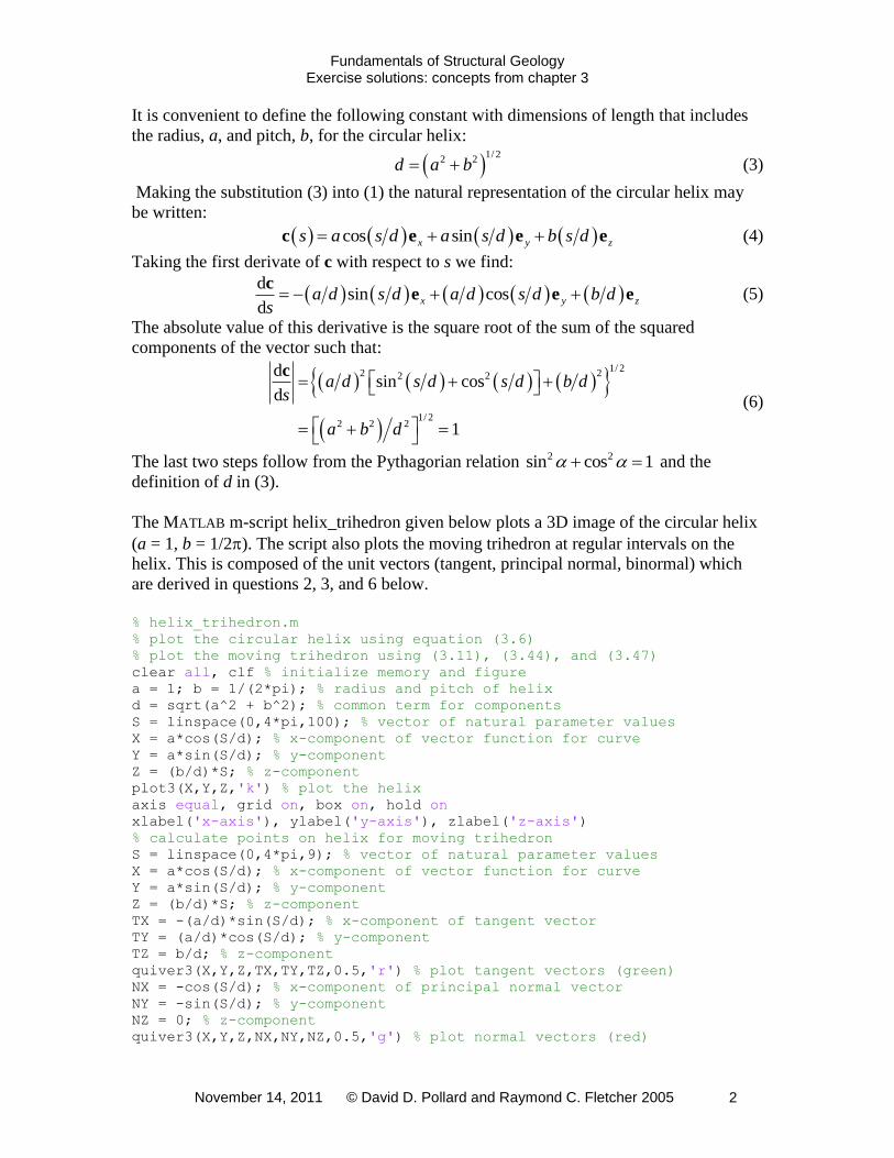
The MATLAB m-script helix_trihedron given below plots a 3D image of the circular helix

(a = 1, b = 1/2). The script also plots the moving trihedron at regular intervals on the

helix. This is composed of the unit vectors (tangent, principal normal, binormal) which

are derived in questions 2, 3, and 6 below.

% helix_trihedron.m % plot the circular helix using equation (3.6) % plot the moving trihedron using (3.11), (3.44), and (3.47) clear all, clf % initialize memory and figure a = 1; b = 1/(2*pi); % radius and pitch of helix d = sqrt(a^2 + b^2); % common term for components S = linspace(0,4*pi,100); % vector of natural parameter values X = a*cos(S/d); % x-component of vector function for curve Y = a*sin(S/d); % y-component Z = (b/d)*S; % z-component plot3(X,Y,Z,'k') % plot the helix axis equal, grid on, box on, hold on xlabel('x-axis'), ylabel('y-axis'), zlabel('z-axis') % calculate points on helix for moving trihedron S = linspace(0,4*pi,9); % vector of natural parameter values X = a*cos(S/d); % x-component of vector function for curve Y = a*sin(S/d); % y-component Z = (b/d)*S; % z-component TX = -(a/d)*sin(S/d); % x-component of tangent vector TY = (a/d)*cos(S/d); % y-component TZ = b/d; % z-component quiver3(X,Y,Z,TX,TY,TZ,0.5,'r') % plot tangent vectors (green) NX = -cos(S/d); % x-component of principal normal vector NY = -sin(S/d); % y-component NZ = 0; % z-component quiver3(X,Y,Z,NX,NY,NZ,0.5,'g') % plot normal vectors (red)



BX = (b/d)*sin(S/d); % x-component of binormal vector BY = -(b/d)*cos(S/d); % y-component BZ = a/d; % z-component quiver3(X,Y,Z,BX,BY,BZ,0.5,'b') % plot binormal vectors (blue)

-0.5

0

0.5

1

-0.5

0

0.5

0

0.2

0.4

0.6

0.8

1

1.2

1.4

1.6

1.8

x-axisy-axis

z-a

xis

Figure 2. Plots of 3D image of the circular helix (a = 1, b = 1/2). Unit tangent vectors

(red), unit principal normal vectors (green), and unit binormal vectors (blue) are

plotted are regular intervals on the helix.

2) An arbitrary representation of a curve, c = c(t), satisfies the condition |dc/dt| = ds/dt,

where t is the arbitrary parameter and s is the natural parameter for the curve.

a) Demonstrate that the following vector function (3.2) is an arbitrary representation

of the circular helix by showing that it satisfies this condition.

cos sin , 0, x y zt a t a t bt a b c e e e (7)

b) Show how this condition and the chain rule are used to derive the equation (3.8)

for the unit tangent vector for an arbitrary representation of a curve and then use

this equation to derive the unit tangent vector for the circular helix (3.11). In the

process show how t and s are related.

c) Using your result from part b) for t(t) write the equation for the unit tangent vector,

t(s), as a function of the natural parameter. Use this equation and MATLAB to plot

a 3D image of a set of unit tangent vectors on the circular helix (a = 1, b = 1/2)

as in Figure 1.

Taking the first derivative of (7) with respect to the parameter t we have:



d

sin cosd

x y za t a t bt

ce e e (8)

The absolute value of this derivative is:

1/ 2 1/ 2

2 2 2 2 2 2dsin cos

da t t b a b d

t

c (9)

Comparing (1) and (7), and using (3), the arbitrary and natural parameters are related as:

1/ 2 1/ 2

2 2 2 2, so t s a b s d s t a b td (10)

Note that t is dimensionless whereas s has dimensions of length. Taking the derivative of

s with respect to t we have:

1/ 2

2 2d

d

sa b d

t (11)

It follows from (9) and (11) that |dc/dt| = ds/dt.

The unit tangent vector is defined as t = dc/ds, but c = c(t) as in (7). Using the Chain Rule

we write:

d d d d d

, so d dd d d

t s

t ts t s

c c ct (12)

but,

d d d d

, so d dd d

s

t tt t

c c ct (13)

For the circular helix, using (13) and substituting from (8) and (9), the unit tangent vector

in terms of the arbitrary parameter t is:

sin cosx y za t a t b d t e e e (14)

Substituting for t in (14) using (10) we have:

sin cosx y za s d a s d b d t e e e (15)

The MATLAB m-script helix_trihedron.m given above plots a 3D image of the circular

helix (a = 1, b = 1/2) with the unit tangent vectors (red) at regular intervals (Figure 2).

3) The curvature vector, scalar curvature, and radius of curvature are three closely related

quantities (Fig. 3.10) that help to describe a curved line in three-dimensional space.

a) Derive equations for the curvature vector, k(s), the scalar curvature, (s), and the

radius of curvature, (s), for the natural representation of the circular helix (1).

b) Show how these equations reduce to the special case of a circle.

c) Derive an equation for the unit principal normal vector, n(s), for the circular helix

as given in (1).

d) Use MATLAB to plot a 3D image (Fig. 1) of a set of unit principal normal vectors

on the circular helix (a = 1, b = 1/2).

e) Derive an equation for the unit binormal vector, b(s), for the circular helix (1). This

is the third member of the moving trihedron.

f) Use MATLAB to plot a 3D image (Fig. 1) of a set of unit binormal vectors on the

circular helix (a = 1, b = 1/2).



The natural representation of the circular helix is written using (3) as:

cos sinx y zs a s d a s d b s d c e e e (16)

The unit tangent vector is the first derivative of c with respect to s:

d

sin cosd

x y zs a d s d a d s d b ds

c

t e e e (17)

The curvature vector is the second derivative of c with respect to s:

2

2 2

2

d dcos sin

d dx ys a d s d a d s d

s s

c tk e e (18)

The scalar curvature is the magnitude of the curvature vector:

1/ 22

2 2 2

1/ 22

2 2

cos sins s a d s d s d

a d a d

k

(19)

Using (3) the scalar curvature for the circular helix is:

2 2a a b (20)

Note that the scalar curvature is a constant. The radius of curvature is the inverse of the

scalar curvature:

2 21 a b a (21)

For the circle b = 0 and d = a, so the curvature vector from (18) reduces to:

1 cos 1 sinx ys a s a a s a k e e (22)

The scalar curvature and radius of curvature from (19) and (21) reduce to:

1 , and a a (23)

The unit principal normal vector is defined in (3.42) as:

ss

s

kn

k (24)

The choice of the sign in the numerator is arbitrary and is used to keep the vector

pointing in a consistent direction along the curve. Using (18) and (19) for the circular

helix and taking the positive sign we have:

2 2 2cos sin

cos sin

x y

x y

s a d s d a d s d a d

s d s d

n e e

e e

(25)

The MATLAB m-script helix_trihedron.m given above plots a 3D image (Figure 2) of the

circular helix (a = 1, b = 1/2) with the unit principal normal vectors (green) at regular

intervals.

From (3.45) the unit binormal vector is defined as:

s s s b t n (26)

From (3.27) the vector (cross) product is given in terms of the respective components as:

y z z y x z x x z y x y y x zs s t n t n t n t n t n t n t n e e e (27)

Substituting for these components from (17) and (25) we have:

sin cosx y zs b d s d b d s d a d b e e e (28)



The MATLAB m-script helix_trihedron.m given above plots a 3D image (Figure 2) of the

circular helix (a = 1, b = 1/2) with the unit binormal vectors (blue) at regular intervals.

4) If c = c(t) is the arbitrary parametric representation of a curve, then a general definition

of the scalar curvature is given in (3.26) as:

32

2

d d d

d d dt

t t t

c c c (29)

a) Show how this relationship may be specialized to plane curves lying in the (x, y)-

plane where c(t) = cxex + cyey and the components are arbitrary functions of t.

b) Further specialize this relationship for the plane curve lying in the (x, y)-plane

where the parameter is taken as x instead of t, so one may write cx = x and cy = f(x)

such that c(x) = xex + f(x)ey and the normal curvature is:

3/ 222

2

d d1

d d

f fx

x x

(30)

c) Evaluate the error introduced in the often-used approximation (x) ~ |d2f/dx

2| by

plotting the following ratio as a function of the slope, df/dx, in MATLAB:

exact approx

exact

(31)

Develop a criterion to limit errors to less than 10% in practical applications.

For the required derivation it is helpful to write the derivatives in a more compact form

using the prime notation. Given the arbitrary representation of a curve, c = c(t), the

equation for the scalar curvature (29) is written:

3

t c c c (32)

Given the plane curve c(t) = cx(t)ex + cy(t)ey the derivatives are expanded as:

, and x x y y x x y yc c c c c e e c e e (33)

The vector (cross) product in the numerator of (32) is found from the following

determinant:

det

0 0

x x x

y y y x y y x z

z

c c

c c c c c c

e

c c e e

e

(34)

The magnitude of this vector is:

1/ 2

2

x y y x x y y xc c c c c c c c

c c (35)

The denominator of (32) is evaluated as:

3

1/ 2 3/ 23 2 22 23

x x y y x y x yc c c c c c

c e e (36)

The scalar curvature is given by the ratio of the right hand sides of (35) and (36):

3/ 2

22

x y y x x yt c c c c c c

(37)



This is (29) specialized for curves lying in the (x, y)-plane where the components and

their derivative are arbitrary functions of t. If the parameter is taken as x instead of t, then

we may write:

1, 0, , x x y yc c c f x c f x (38)

Substituting (38) into (37) and writing out the derivatives the scalar curvature is:

3/ 222

2

d d1

d d

f fx

x x

(39)

This is the form of the scalar curvature often introduced in elementary calculus courses.

Using the prime notation for derivatives in (39), the exact and approximate scalar

curvatures are written:

3/ 2

2exact 1 , approxf f f

(40)

Note that the approximate scalar curvature is obtained by postulating:

2

1 1f (41)

In other words the square of the first derivative of the function y = f(x) is small compared

to one. Substituting (40) into (31) the error is written:

3/ 22

1 1exact approx

fexact

(42)

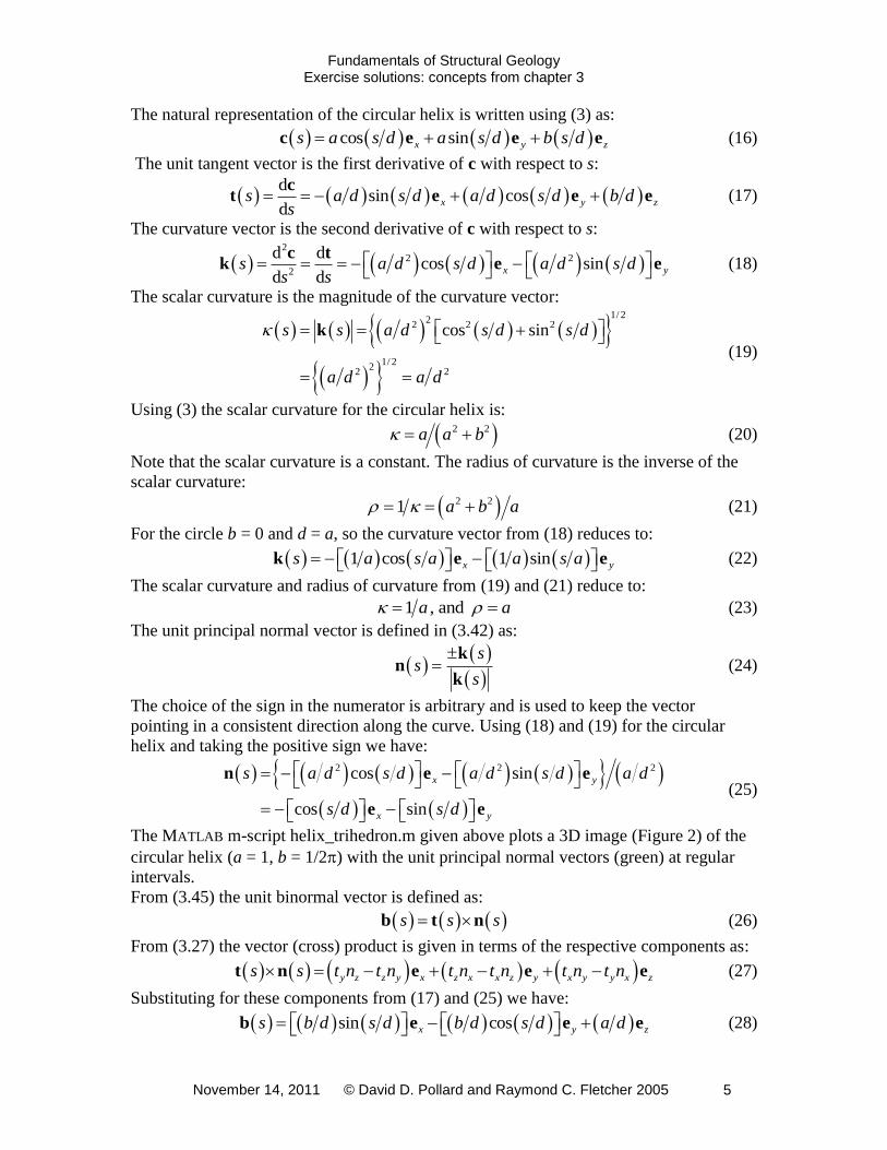
The slope of the curve y = f(x) is given by the first derivative f’(x) and the angle of the

slope is (180/)f’(x). The absolute value of this error is plotted versus the slope angle of

the curve using the MATLAB m-script curve_approx.m:

% curve_approx.m % evaluation of error for plane curvature approximation clear all, clf, hold on % initialize S = linspace(0,pi/4,100); % slope values (radians) E = abs(1 - ((1 + S.^2).^(3/2))); % absolute value of error plot(S*180/pi,E*100) % plot in 2D plot ([0 45], [10 10],'r--') grid on, box on xlabel('slope (degrees)'), ylabel('|error| (percent)')

From reading the graph in Figure 3, for slopes less than about 15 degrees, the absolute

value of the error is less than about 10 percent. This error threshold is quantified using

(42) such that:

3/ 2

21 1 0.1f

(43)

Rearranging:

3/ 2

21 1.1f

(44)

Solving for the magnitude of f’ we have:

2/3

1.1 1 0.256f (45)



Recalling that f’ is the tangent of the slope of the curve, this threshold restricts the range

of slope angles, , such that:

14.37 14.37o o (46)

Figure 3. Plot of the absolute value of the error introduced in the approximation for the

curvature is plotted versus the slope angle of the curve.

The approximation is reasonable for surfaces with slopes less than about 15 degrees but

the error increases rapidly with slope reaching about 100% at 45 degrees.

5) If c = c(t) is the arbitrary parametric representation of a curve, then a general definition

of the scalar torsion is given is (3.50) as:

22 3 2

2 3 2

d d d d d( )

d d d d dt

t t t t t

c c c c c (47)

a) Derive an expression for the scalar torsion for the parametric representation of the

circular helix of radius a and pitch b as given by:

cos sin , 0, x y zt a t a t bt a b c e e e (48)

The scalar torsion (47) is written using the prime notation as:

2

( )t c c c c c (49)

The derivatives in (49) for the case of the circular helix are:



sin cos

cos sin

sin cos

x y z

x y

x y

t a t a t b

t a t a t

t a t a t

c e e e

c e e

c e e

(50)

The numerator of (49) is a triple scalar product which may be evaluated using (3.51):

det

x x x

y y y

z z z

x y z z y y z x x z z x y y x

c c c

c c c c c c

c c c

c c c c c c c c c c c c c c c

(51)

Of the three terms on the right side of (51) only the last survives because 0z z c c as

seen from the second and third of (50). The triple product for the helix evaluates to:

2 2 2 2 2cos sinz x y y x b a t a t ba c c c c c c c c (52)

The vector product in the denominator of (49) evaluates using the following determinant:

det

x x xx

y y y

z z z

y zz zz yy x zz xxx xx z y xx y y xxx z

e c c

c c e c c

e c c

c c c c e c c c c e c c c c e

(53)

Noting from the second of (50) that 0z c for the circular helix this vector product

evaluates to:

2sin cos

zz yy x z x y xx y y xxx z

x y zab t ab t a

c c c c e c c e c c c c e

e e e (54)

The square of the absolute value of (54) is:

22 2 2 4 2 2 2sin cosab t t a a a b

c c (55)

The ratio of (52) and (55) is the scalar torsion:

2 2b a b (56)

Note that the scalar torsion for the circular helix is a constant.

6) The two intrinsic scalar properties of continuous curves are the curvature (3.20) and

the torsion (3.48). For the circular helix these properties are constants given by:

2 2 2 2, a a b b a b (57)

a) Use MATLAB to plot two 3D graphs, one for the scalar curvature and the other for

the torsion. Use a range for the radius, a, of 0 ≤ a ≤ 3 and for the pitch, b of –1.5 ≤

b ≤ +1.5. Study your graphs and describe the interesting features.

The MATLAB m-script helix_cur_tor.m plots a 3D image of the scalar curvature, , and

another for the scalar torsion, , using the ranges specified above. % helix_cur_tor.m % plot scalar curvature and torsion clear all, clf % initialize



a = linspace(0,3,30); % vector of values for radius b = linspace(-1.5,1.5,30); % vector of values for pitch [A,B]=meshgrid(a,b); % grid of points C = A./(A.^2 + B.^2); % scalar curvature R=sqrt(A.^2 + B.^2); C(find(R<0.20)) = nan; % exclude calculations very near (0, 0) mesh(A,B,C) % plot surface as wire-frame xlabel('Radius, a'), ylabel('Pitch, b'), zlabel('Scalar Curvature') title('Curvature of Right Circular Helix') axis equal, axis([0 3 -1.5 1.5 0 3]) T = B./(A.^2 + B.^2); % scalar torsion T(find(R<0.20)) = nan; % exclude calculations very near (0, 0) figure, mesh(A,B,T) % plot surface as wire-frame xlabel('Radius, a'), ylabel('Pitch, b'), zlabel('Scalar Torsion') title('Torsion of Right Circular Helix') axis equal, axis([0 3 -1.5 1.5 -1.5 1.5])

From studying Figure 4 and recalling that for b = 0, = 1/a, there is a positive

singularity in the scalar curvature as a → 0. Except in the neighborhood of this point →

0 as a → 0 and the helix degenerates into a straight line.

From studying Figure 5 and recalling that for a = 0, = 1/b, there is a positive and

negative singularity in the scalar torsion as b → 0. For b = 0, = 0 except in the

neighborhood of these singularities. For b << a, as a increases the torsion decreases

toward zero with a sign given by the sign of b.

0

1

2

3

-1.5

-1

-0.5

0

0.5

1

1.5

0

0.5

1

1.5

2

2.5

3

Radius, a

Curvature of Right Circular Helix

Pitch, b

Sca

lar

Cu

rva

ture

Figure 4. 3D plot of the scalar curvature using a range for the radius, a, of 0 ≤ a ≤ 3 and

for the pitch, b of –1.5 ≤ b ≤ +1.5 for the circular helix.



0

1

2

3

-1.5

-1

-0.5

0

0.5

1

1.5

-1.5

-1

-0.5

0

0.5

1

1.5

Radius, a

Torsion of Right Circular Helix

Pitch, b

Sca

lar

To

rsio

n

Figure 5. 3D plot of the scalar torsion using a range for the radius, a, of 0 ≤ a ≤ 3 and for

the pitch, b of –1.5 ≤ b ≤ +1.5 for the circular helix.

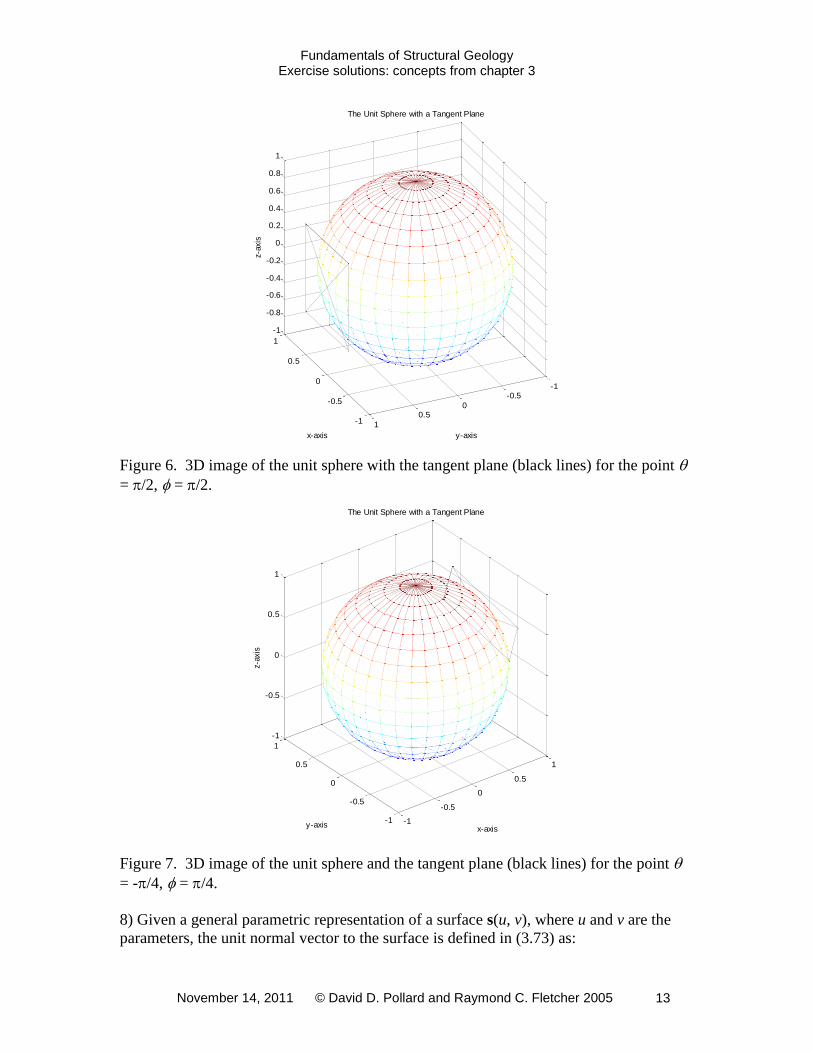
7) The tangent plane at a point on a surface is illustrated in Figure 3.19. For geological

surfaces it is the orientation of the tangent plane at a point on the surface that is measured

using strike and dip. Given a general parametric representation of a surface s(u, v), where

u and v are scalar quantities that are the parameters of the surface, the tangent plane to the

surface is defined in (3.63) as:

, ,h k h ku v

s sP s (58)

As an example consider the parametric representation of the sphere of radius a given

using the two parameters, and :

, cos sin sin sin cos

0 , 0 2 , 0

x y za a a

a

s e e e (59)

a) Derive the general equations for the tangent plane, P, to this sphere.

b) Evaluate your equation for the particular case of the point = /2, = /2 and

explain how your result matches (or not) your intuition.

c) Use MATLAB to plot the sphere and a portion of the tangent plane at the point =

/2, = /2. Also, plot the tangent plane at the point = -/4, = /4.

For the sphere defined in (59) the first partial derivatives of s( ,) are:

sin sin cos sin

cos cos sin cos sin

x y

x y z

a a

a a a

se e

se e e

(60)



For the point = /2, = /2 the tangent plane is found by substituting these values into

(59) and (60) and then inserting the resulting expressions into (58) to find:

2 2, y x za ha ka P e e e (61)

The first term on the right side locates the point at the intersection of the sphere and the

positive y-axis. As h and k vary the second and third terms trace out a plane through this

point that is parallel to the (x, z)-coordinate plane.

The MATLAB m-script sphere_tangent_plane.m plots a 3D image of the unit sphere and

the tangent plane according to (61). The second plot is obtained by changing the values of

the parameters.

% sphere_tangent_plane.m % plot the unit sphere as a wireframe 3D plot with a tangent plane clear all; clf reset; % clear variables and figures a = 1; m = 37; n = 19; % sphere radius, number of long. and lat. points th = linspace(0,2*pi,m); % theta (long) coordinates on parameter plane ph = linspace(0,pi,n); % phi (lat) coordinatess on parameter plane [TH,PH]=meshgrid(th,ph); % grid of points on parameter plane NX = a*cos(TH).*sin(PH); % x-component of radius vector NY = a*sin(TH).*sin(PH); % y-component of radius vector NZ = a*cos(PH); % z-component of radius vector mesh(NX,NY,NZ) % 3D mesh surface plot of unit sphere xlabel('x-axis'), ylabel('y-axis'), zlabel('z-axis') title('The Unit Sphere with a Tangent Plane') axis equal, hold on tht = pi/2; pht = pi/2; % coordinates of point, s, for tangent plane h = 0.5*a; k = 0.5*a; H = [h,-h,-h,h,h,-h,h,-h]; K = [k,k,-k,-k,k,-k,-k,k]; sx = a*cos(tht)*sin(pht); % vector components for s sy = a*sin(tht)*sin(pht); sz = a*cos(pht); dstx = -a*sin(tht)*sin(pht); % vector components of tangent vector dsty = a*cos(tht)*sin(pht); dspx = a*cos(tht)*cos(pht); % vector components of tangent vector dspy = a*sin(tht)*cos(pht); dspz = -a*sin(pht); X = sx + H*dstx + K*dspx; Y = sy + H*dsty + K*dspy; Z = sz + K*dspz; plot3(X,Y,Z,'k-') % plot a portion of the tangent plane



-1

-0.5

0

0.5

1

-1-0.5

00.5

1

-1

-0.8

-0.6

-0.4

-0.2

0

0.2

0.4

0.6

0.8

1

y-axis

The Unit Sphere with a Tangent Plane

x-axis

z-a

xis

Figure 6. 3D image of the unit sphere with the tangent plane (black lines) for the point

= /2, = /2.

-1

-0.5

0

0.5

1

-1

-0.5

0

0.5

1

-1

-0.5

0

0.5

1

x-axis

The Unit Sphere with a Tangent Plane

y-axis

z-a

xis

Figure 7. 3D image of the unit sphere and the tangent plane (black lines) for the point

= -/4, = /4.

8) Given a general parametric representation of a surface s(u, v), where u and v are the

parameters, the unit normal vector to the surface is defined in (3.73) as:



u v u v

s s s sN (62)

a) Derive the equation for the unit normal vector, N, for the sphere of radius a with

the parametric representation:


0 , 0 2 , 0

x y za a a

a

s e e e (63)

b) Show that your equation for N obeys the condition N = -s/a, where s(, ) is the

position vector for a point on the sphere from an origin at the center of the sphere.

For the sphere of radius a defined in (63) the first partial derivatives are:

sin sin cos sin

cos cos sin cos sin

x y

x y z

a a

a a a

se e

se e e

(64)

The vector product of these derivatives is found from the general definition for two

arbitrary vectors, u and w, as given in (3.27):

y z z y x z x x z y x y y x zv w v w v w v w v w v w v w e e e (65)

Substituting the components from (64) into (65) we find:

cos sin sin sin sin sin

sin sin sin cos cos sin cos cos

x y

z

a a a a

a a a a

s se e

e

(66)

Combining terms:

2 2 2 2 2cos sin sin sin sin cosx y za a a

s se e e (67)

The absolute value of the vector product is:

1/ 24 2 4 2 4 2 2

1/ 22 2 2 2 2

cos sin sin sin sin cos

sin sin cos sin

a

a a

s s

(68)

Taking the ratio of (67) and (68) we have the unit normal vector for the sphere:

cos sin sin sin cosx y z N e e e (69)

The position vector for a point on the sphere is given in (59):

, cos sin sin sin cosx y za a a s e e e (70)

Comparing (69) and (70) we have N = -s/a.

c) Given orientation data from a field measurement of strike and dip (s, s) of a

bedding surface, show how these angles would be converted to the trend and

plunge (n, n) of the normal to that bed. Then show how these angles are used to

compute the components of the unit normal vector for the bedding surface.



9) The coefficients of the first fundamental form are used to calculate arc lengths of

curves. The coefficients of the first fundamental form are defined in (3.85) as:

, , E F Gu u u v v v

s s s s s s (71)

The arc length of a curve c[u(t), v(t)] on a surface, s(u,v) is defined in (3.89) as:

1/ 22 2

2

b

a

du du dv dvs E F G dt

dt dt dt dt

(72)

As an example consider the parametric representation of the elliptic paraboloid:

2 2, x y zu v u v u v s e e e (73)

a) Consider the u-parameter curve c(u, 0.7) and calculate the arc length of this

parabola from u = -1m to u = +1m.

b) Use MATLAB to plot the elliptic paraboloid (73) and the parabolic curve c(u, 0.7).

For the circular paraboloid defined in (73) the coefficients are:

2

2

2 2 1 4

2 2 1 4

2 2 1 4

x z x z

x z y z

y z y z

E u u u

F u v uv

G v v v

e e e e

e e e e

e e e e

(74)

For a u-parameter curve u = t and v = constant, so du/dt = 1 and dv/dt = 0. In this case the

limits of integration are a = -1m and b = +1m, and dt = du. Making these substitutions in

(72) we have:

1 11/ 2 1/ 2

2 2

1 0

1 4 2 1 4s u du u du

(75)

From Jeffrey, p. 158 (or similar table of integrals):

1/ 2 1/ 2 1/ 2

2 2 21 1 12 2

ln , 0c

a cx dx x a cx a x c a cx c (76)

Here a = 1, c = 4, and x = u so:

1

1/ 2 1/ 22 21 1

2 2

0

1 4 ln 2 1 4 5 ln 2 5 2.958ms u u u u

(77)

The MATLAB m-script circ_paraboloid.m plots a 3D image of the circular paraboloid and

the u-parameter curve c(u, 0.7).

% circ_paraboloid u = linspace(-1,1,21); % vector of u-coords on parameter plane v = linspace(-1,1,21); % vector of v-coords on parameter plane [U,V]=meshgrid(u,v); % grid of points on parameter plane SX = U; % x-component of vector function for surface, s=f(u,v) SY = V; % y-component of s=f(u,v) SZ = U.^2 + V.^2; % z-component of s=f(u,v) surf(SX,SY,SZ) % surface plot: wire-frame with color fill xlabel('x-axis'), ylabel('y-axis'), zlabel('z-axis') title('surface plot: elliptic paraboloid'), axis equal figure, plot(u,SZ(18,1:21)) %plot u-parameter curve c(u,0.7)



xlabel('x-axis'), ylabel('z-axis') title('u-parameter curve on elliptic paraboloid, v = 0.7') axis equal, axis([-1 1 0 2])

-1

-0.5

0

0.5

1

-1

-0.5

0

0.5

1

0

0.5

1

1.5

2

x-axis

surface plot: elliptic paraboloid

y-axis

z-a

xis

Figure 8. 3D image of the circular paraboloid.

-1 -0.8 -0.6 -0.4 -0.2 0 0.2 0.4 0.6 0.8 10

0.2

0.4

0.6

0.8

1

1.2

1.4

1.6

1.8

2

x-axis

z-a

xis

u-parameter curve on elliptic paraboloid, v = 0.7

Figure 9. Plot of the u-parameter curve c(u, 0.7) to the circular paraboloid.



10) The coefficients of the first fundamental form may be used to calculate surface area

(Fig. 3.26) given the parametric representation of a surface. The general equation for the

surface area in terms of the parametric representation s(u,v) and the coefficients of the

first fundamental form is given in (3.95) as:

1/ 2

2 d dA EG F u v (78)

Consider the following representation of the sphere of radius a:


0 , 0 2 , 0

x y za a a

a

s e e e (79)

a) Derive an equation for the surface area of the sector of the sphere within the range

0 ≤ ≤ /4 and < ≤ and evaluate this for a = 1m.

b) Plot this sector of the sphere in 3D using MATLAB.

For the sphere, s(, ), defined in (79) the surface area is calculated using (78) such that:

1/ 2

2

4 6, 0 , 0A EG F d d (80)

The coefficients of the first fundamental form are given in (3.85) as:

, , E F G

s s s s s s (81)

The first partial derivatives of s(, ) are:

sin sin cos sin

cos cos sin cos sin

x y

x y z

a a

a a a

se e

se e e

(82)

Uisng (82) in (81) the coefficients of the first fundamental form are:

2 2 2 2 2 2 2 2

2 2

2 2 2 2 2 2 2 2 2

sin sin cos sin sin

sin cos sin cos sin cos sin cos 0

cos cos sin cos sin

E a a a

F a a

G a a a a

(83)

Therefore, the integrand of (80) is:

1/ 2

2 2 sinEG F a (84)

The integral is evaluated over the specified ranges as:

/ 4 / 6 / 4/ 62 2

00 0 0

2/ 42 23 3

2 20

sin d d cos d

1 1 0.105m4

A a a

aa

(85)

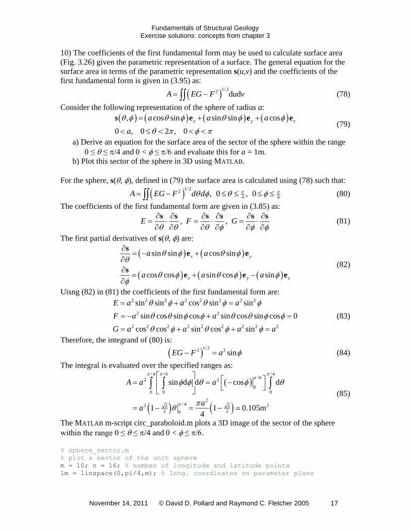
The MATLAB m-script circ_paraboloid.m plots a 3D image of the sector of the sphere

within the range 0 ≤ ≤ /4 and < ≤ .

% sphere_sector.m % plot a sector of the unit sphere m = 10; n = 16; % number of longitude and latitude points lm = linspace(0,pi/4,m); % long. coordinates on parameter plane



ph = linspace(0+eps,pi/6,n); % lat. coordinates on parameter plane [LM,PH]=meshgrid(lm,ph); % grid of points on parameter plane NX = cos(LM).*sin(PH); % x-component of radius vector NY = sin(LM).*sin(PH); % y-component of radius vector NZ = cos(PH); % z-component of radius vector figure, mesh(NX,NY,NZ) % 3D mesh surface plot of unit sphere xlabel('x-axis'), ylabel('y-axis'), zlabel('z-axis') title('Sector of the Unit Sphere'), axis equal axis([0 .5 0 .5 .8 1])

0

0.1

0.2

0.3

0.4

0.5

0

0.1

0.2

0.3

0.4

0.5

0.8

0.85

0.9

0.95

1

x-axis

Sector of the Unit Sphere

y-axis

z-a

xis

Figure 10. 3D image of the sector of the sphere within the range 0 ≤ ≤ /4 and < ≤

.

11) The general equation for the unit normal vector to a surface with the parametric

representation s(u,v) is given in (3.73) as:

u v u v

s s s sN (86)

As an example consider the surface with the parametric representation:

2 2, x y zu v u v u v s e e e (87)

a) Use MATLAB to plot a 3D illustration of this surface as a wire frame or other

suitable graph and describe the shape. This is the hyperbolic paraboloid (Fig.

3.29c).

b) Derive an equation for the unit normal vector, (u, v), of the hyperbolic paraboloid

given in (87). Compare your equation to (3.75) which is the unit normal vector of

the elliptic paraboloid and describe the differences.

c) Use MATLAB to plot the unit normal vectors on the hyperbolic paraboloid.



The MATLAB m-script hyperbolic_paraboloid.m plots a 3D image of the surface (87).

% hyperbolic_paraboloid.m % plot hyperbolic paraboloid and normal vectors u = linspace(-1,1,21); % vector of u-coords on parameter plane v = linspace(-1,1,21); % vector of v-coords on parameter plane [U,V]=meshgrid(u,v); % grid of points on parameter plane SX = U; % x-component of vector function for surface, s=f(u,v) SY = V; % y-component of s=f(u,v) SZ = U.^2 - V.^2; % z-component of s=f(u,v) surf(SX,SY,SZ) % surface plot: wire-frame with color fill xlabel('x-axis'), ylabel('y-axis'), zlabel('z-axis') title('surface plot: hyperbolic paraboloid'), axis equal D = sqrt(1+4*U.^2+4*V.^2); % calculate unit normal vector NX = -2*U./D; NY = 2*V./D; NZ = 1./D; figure, mesh(SX,SY,SZ) % mesh plot: wire-frame xlabel('x-axis'), ylabel('y-axis'), zlabel('z-axis') title('hyperbolic paraboloid with normals'), axis equal, hold on quiver3(SX,SY,SZ,NX,NY,NZ) % plot unit normal vectors

-1

-0.5

0

0.5

1

-1

-0.5

0

0.5

1

-1

-0.5

0

0.5

1

x-axis

surface plot: hyperbolic paraboloid

y-axis

z-a

xis

Figure 11. 3D illustration of the hyperbolic paraboloid.

For the hyperbolic paraboloid (87) the first partial derivatives are:

2 , 2x z y zu vu v

s se e e e (88)

The numerator in (86) is evaluated using (88) such that:

1 0

det 0 1 2 2

2 2

x

y x y z

z

u vu v

u v

es s

e e e e

e

(89)



The absolute value of this vector product is:

1/ 2

2 24 4 1u vu v

s s (90)

The unit normal vector for the hyperbolic hyperboloid is the ratio of (89) and (90):

1/ 2

2 22 2 4 4 1x y zu v u v N e e e (91)

The unit normal vector for the elliptic paraboloid from (3.75) is:

1/ 2

2 22 2 4 4 1x y zu v u v N e e e (92)

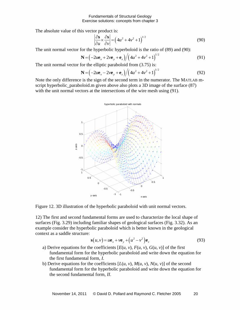
Note the only difference is the sign of the second term in the numerator. The MATLAB m-

script hyperbolic_paraboloid.m given above also plots a 3D image of the surface (87)

with the unit normal vectors at the intersections of the wire mesh using (91).

-1

-0.5

0

0.5

1

-1

-0.5

0

0.5

1

-1

-0.5

0

0.5

1

x-axis

hyperbolic paraboloid with normals

y-axis

z-a

xis

Figure 12. 3D illustration of the hyperbolic paraboloid with unit normal vectors.

12) The first and second fundamental forms are used to characterize the local shape of

surfaces (Fig. 3.29) including familiar shapes of geological surfaces (Fig. 3.32). As an

example consider the hyperbolic paraboloid which is better known in the geological

context as a saddle structure:

2 2, x y zu v u v u v s e e e (93)

a) Derive equations for the coefficients [E(u, v), F(u, v), G(u, v)] of the first

fundamental form for the hyperbolic paraboloid and write down the equation for

the first fundamental form, I.

b) Derive equations for the coefficients [L(u, v), M(u, v), N(u, v)] of the second

fundamental form for the hyperbolic paraboloid and write down the equation for

the second fundamental form, II.



c) Use the coefficients of the second fundamental form to identify whether the point

on the hyperbolic paraboloid at the origin (x = y = z = 0) is elliptic, hyperbolic,

parabolic or planar. What can you conclude about the shape at an arbitrary point

on the hyperbolic paraboloid?

d) The normal curvature, n, for a surface is given in (3.120) by the ratio of the two

fundamental forms, n = II/I. Derive an equation for the normal curvature of the

hyperbolic paraboloid in terms of the parameters (u, v) and their differentials (du,

dv). Use the equation for n to determine the normal curvature at the origin (x = y

= z = 0) for this surface.

e) Plot the distribution of normal curvature at the origin as a function of orientation

using MATLAB. Hint: consider the circular path around the origin defined by du2 +

dv2 = 1, and plotn versus the angle measured from the u-axis. Identify the values

of the principal normal curvatures and the principal directions at the origin.

The coefficients of the first fundamental form for the parametric representation of a

surface s(u,v) are given in (3.85) as:

, , E F Gu u u v v v

s s s s s s (94)

For the hyperbolic paraboloid (93) the first partial derivatives are:

2 , 2x z y zu vu v

s se e e e (95)

Using (95) in (94) the coefficients of the first fundamental form are:

2

2

2 2 1 4

2 2 4

2 2 1 4

x z x z

x z y z

y z y z

E u u u

F u v uv

G v v v

e e e e

e e e e

e e e e

(96)

The general equation for the first fundamental form for the parametric representation of a

surface s(u,v) is given in (3.85) as:

2 2d 2 d d dI E u F u v G v (97)

For the hyperbolic paraboloid the first fundamental form is:

2 2 2 21 4 d 8 d d 1 4 dI u u uv u v v v (98)

The general equations for the coefficients of the second fundamental form for the

parametric representation of a surface s(u,v) are given in (3.109) as:

2 2 2

2 2, , L M N

u u v v

s s sN N N (99)

The unit normal vector for the hyperbolic paraboloid is given in (91) as:

1/ 2

2 22 2 4 4 1x y zu v u v N e e e (100)

The second partial derivatives are found using (95) such that:

2 2 2

2 22 , 0, 2z z

u u v v

s s se e (101)

Taking the scalar products of the unit normal vector and the appropriate second partial

derivative as indicated in (99), the coefficients of the second fundamental form are:



1/ 2 1/ 2

2 2 2 22 4 4 1 , 0, 2 4 4 1L u v M N u v (102)

The general equation for the second fundamental form for the parametric representation

of a surface s(u,v) as given in (3.106) is:

2 2d 2 d d dII L u M u v N v (103)

The second fundamental form for the hyperbolic paraboloid is written using the

coefficients (102) as:

1/ 2

2 2 2 22d 2d 4 4 1II u v u v (104)

The shape of a surface at a given point to second order is determined by the combination

of coefficients LN – M2 as described in (3.110). For the hyperbolic paraboloid we have:

2 2 24 4 4 1LN M u v (105)

At the origin of the coordinate system the shape is determined by:

2 4, at 0 , 0LN M x u y v (106)

Because the combination of coefficients is negative this is a hyperbolic point. In general,

from (105) we see that all points are hyperbolic.

The normal curvature for the hyperbolic paraboloid is found from (98) and (104) such

that:

1/ 22 2 2 2

2 2 2 2

2d 2d 4 4 1

1 4 d 8 d d 1 4 dn

u v u vII

I u u uv u v v v

(107)

At the origin of coordinates the normal curvature is:

2 2

2 2

2 d d, at 0 , 0

d dn

u vx u y v

u v

(108)

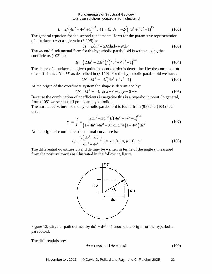
The differential quantities du and dv may be written in terms of the angle measured

from the positive x-axis as illustrated in the following figure:

Figure 13. Circular path defined by du2 + dv

2 = 1 around the origin for the hyperbolic

paraboloid.

The differentials are:

cos and sindu dv (109)



The circular path is written:

2 2 2 2d d cos sin 1u v (110)

The normal curvature from (108) is:

2 22 cos sin 2cos2n (111)

The MATLAB m-script hyper_para.m plots a 2D distribution of the normal curvature at

the orgin.

% hyper_para.m % plot the distribution of normal curvature at the origin TH = 0:pi/180:2*pi; THD = TH*180/pi; % Angle theta figure, plot(THD,2*(cos(TH).^2 -sin(TH).^2)) axis([0 360 -2.5 2.5])

0 50 100 150 200 250 300 350-2.5

-2

-1.5

-1

-0.5

0

0.5

1

1.5

2

2.5

Figure 14. 2D distribution of the normal curvature at the orgin for the hyperbolic

paraboloid.

Exercise solutions: concepts from chapter 3

Documents

Transcript of Exercise solutions: concepts from chapter 3