Exercise 1 – table under static loading€¦ · exercise and the tutorial is valid. Preparing the...

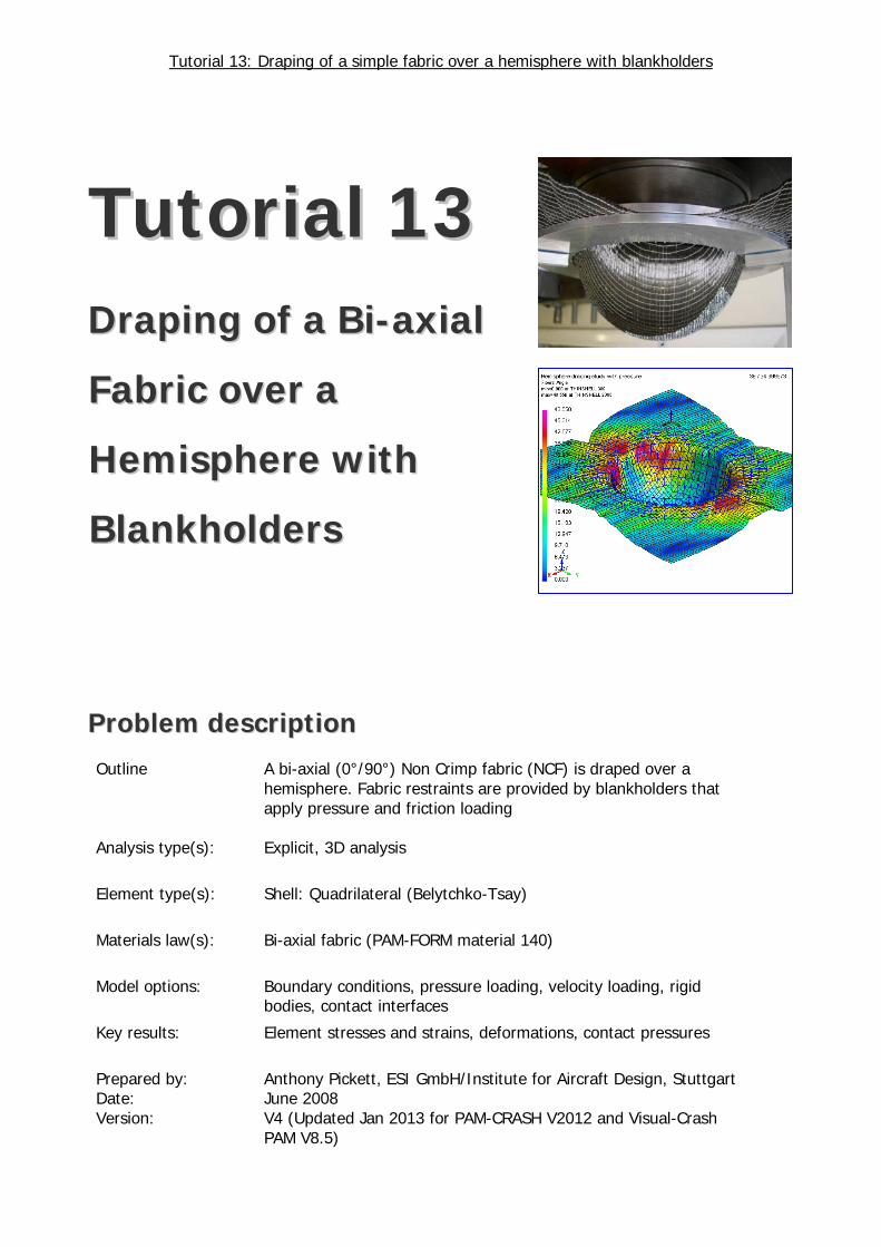
Tutorial 13: Draping of a simple fabric over a hemisphere with blankholders

TTuuttoorriiaall 1133

DDrraappiinngg ooff aa BBii--aaxxiiaall

FFaabbrriicc oovveerr aa

HHeemmiisspphheerree wwiitthh

BBllaannkkhhoollddeerrss

PPrroobblleemm ddeessccrriippttiioonn Outline A bi-axial (0°/90°) Non Crimp fabric (NCF) is draped over a

hemisphere. Fabric restraints are provided by blankholders that apply pressure and friction loading

Analysis type(s): Explicit, 3D analysis

Element type(s): Shell: Quadrilateral (Belytchko-Tsay)

Materials law(s): Bi-axial fabric (PAM-FORM material 140)

Model options: Boundary conditions, pressure loading, velocity loading, rigid bodies, contact interfaces

Key results: Element stresses and strains, deformations, contact pressures

Prepared by: Date: Version:

Anthony Pickett, ESI GmbH/Institute for Aircraft Design, Stuttgart June 2008 V4 (Updated Jan 2013 for PAM-CRASH V2012 and Visual-Crash PAM V8.5)


Upper blankholder

Background information

Pre-processor, Solver and Post-processor used:

• Visual-Mesh: For generation of the geometry and meshes.

• Visual-Crash PAM: To assign control, material data, loadings, constraints, contacts, time history and analysis control data.

• Analysis (PAM-FORM Explicit): To perform the explicit Finite Element analysis.

Note that this analysis uses the PAM-CRASH code with a PAM-FORM licence to use the fabric draping material model (140); this provides advantages in the range of modelling options that can be used. For more complex thermoforming draping analysis, with temperature, the full PAM-FORM and model preparation software’s must be used.

• Visual-Viewer: To evaluate the results of contour plots, deformations, fibre angles, etc. Prior knowledge for the exercise No prior Visual or PAM-Form knowledge is required for working through this exercise.

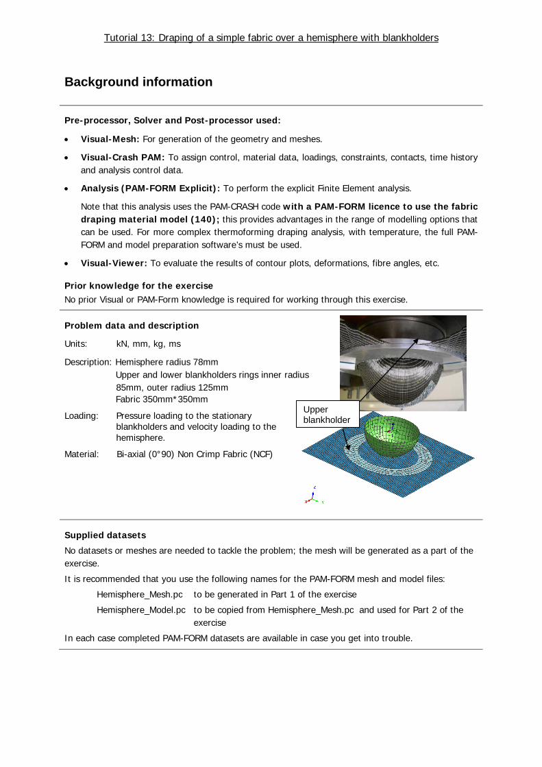
Problem data and description

Units: kN, mm, kg, ms

Description: Hemisphere radius 78mm Upper and lower blankholders rings inner radius

85mm, outer radius 125mm Fabric 350mm*350mm

Loading: Pressure loading to the stationary blankholders and velocity loading to the hemisphere.

Material: Bi-axial (0°90) Non Crimp Fabric (NCF)

Supplied datasets

No datasets or meshes are needed to tackle the problem; the mesh will be generated as a part of the exercise.

It is recommended that you use the following names for the PAM-FORM mesh and model files:

Hemisphere_Mesh.pc to be generated in Part 1 of the exercise

Hemisphere_Model.pc to be copied from Hemisphere_Mesh.pc and used for Part 2 of the exercise

In each case completed PAM-FORM datasets are available in case you get into trouble.


Part 1: Using VCP to make the hemisphere, blankholder and fabric meshes

Note: Some panels shown to construct and post-process the model are old and refer to Visual

version 4.0, some are new (Visual V8.5). Never-the-less it is possible to work through the exercise and the tutorial is valid.

Preparing the mesh (Visual Mesh)

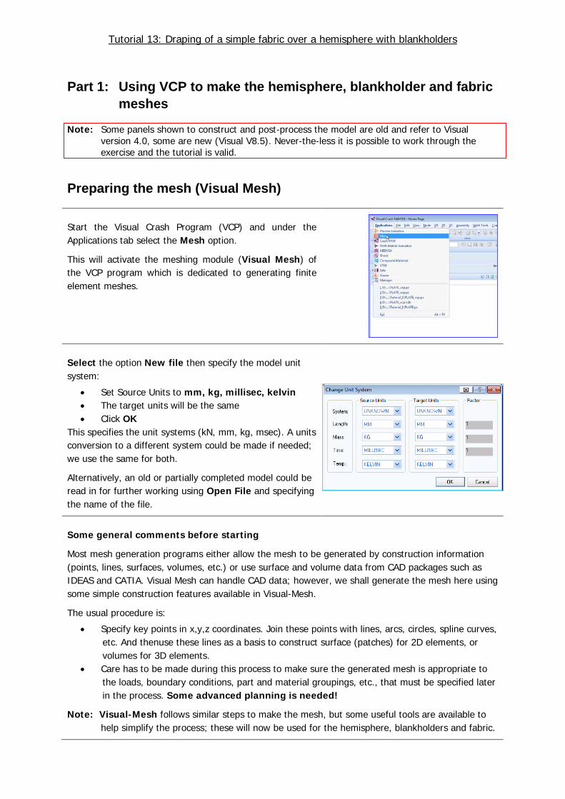
Start the Visual Crash Program (VCP) and under the Applications tab select the Mesh option.

This will activate the meshing module (Visual Mesh) of the VCP program which is dedicated to generating finite element meshes.

Select the option New file then specify the model unit system:

• Set Source Units to mm, kg, millisec, kelvin • The target units will be the same • Click OK

This specifies the unit systems (kN, mm, kg, msec). A units conversion to a different system could be made if needed; we use the same for both.

Alternatively, an old or partially completed model could be read in for further working using Open File and specifying the name of the file.

Some general comments before starting

Most mesh generation programs either allow the mesh to be generated by construction information (points, lines, surfaces, volumes, etc.) or use surface and volume data from CAD packages such as IDEAS and CATIA. Visual Mesh can handle CAD data; however, we shall generate the mesh here using some simple construction features available in Visual-Mesh.

The usual procedure is:

• Specify key points in x,y,z coordinates. Join these points with lines, arcs, circles, spline curves, etc. And thenuse these lines as a basis to construct surface (patches) for 2D elements, or volumes for 3D elements.

• Care has to be made during this process to make sure the generated mesh is appropriate to the loads, boundary conditions, part and material groupings, etc., that must be specified later in the process. Some advanced planning is needed!

Note: Visual-Mesh follows similar steps to make the mesh, but some useful tools are available to help simplify the process; these will now be used for the hemisphere, blankholders and fabric.


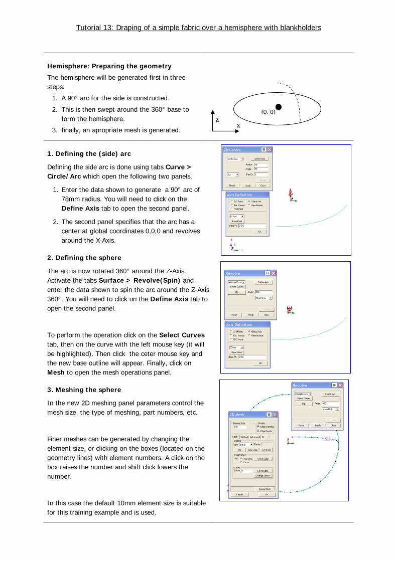
Hemisphere: Preparing the geometry

The hemisphere will be generated first in three steps:

1. A 90° arc for the side is constructed.

2. This is then swept around the 360° base to form the hemisphere.

3. finally, an apropriate mesh is generated.

1. Defining the (side) arc

Defining the side arc is done using tabs Curve > Circle/Arc which open the following two panels.

1. Enter the data shown to generate a 90° arc of 78mm radius. You will need to click on the Define Axis tab to open the second panel.

2. The second panel specifies that the arc has a center at global coordinates 0,0,0 and revolves around the X-Axis.

2. Defining the sphere

The arc is now rotated 360° around the Z-Axis. Activate the tabs Surface > Revolve(Spin) and enter the data shown to spin the arc around the Z-Axis 360°. You will need to click on the Define Axis tab to open the second panel.

To perform the operation click on the Select Curves tab, then on the curve with the left mouse key (it will be highlighted). Then click the ceter mouse key and the new base outline will appear. Finally, click on Mesh to open the mesh operations panel.

3. Meshing the sphere

In the new 2D meshing panel parameters control the mesh size, the type of meshing, part numbers, etc.

Finer meshes can be generated by changing the element size, or clicking on the boxes (located on the geometry lines) with element numbers. A click on the box raises the number and shift click lowers the number.

In this case the default 10mm element size is suitable for this training example and is used.

x z

(0, 0)


Click on Create Mesh and OK.

The adjacent mesh is created.

Positioning and viewing options:

Important options are available in the main (top) panel to position, center, zoom (in and out) and gererally vary viewing of the model.

1. Click the axis tab and with the ‘left’ mouse key to open options to position the model in the x,y,z or perspective (isometric) frame.

2. Click the viewing tab with the ‘left’ mouse key to open options to zoom in/out and generally position the model.

Spend 2-3 minutes to be familiar with these options; they are important. Use tab options (1) and (2) to center and position the model in isometric view.

(1) (2)


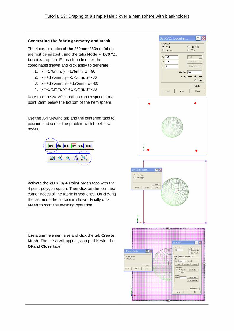
Generating the fabric geometry and mesh

The 4 corner nodes of the 350mm*350mm fabric are first generated using the tabs Node > ByXYZ, Locate… option. For each node enter the coordinates shown and click apply to generate:

1. x=-175mm, y=-175mm, z=-80 2. x=+175mm, y=-175mm, z=-80 3. x=+175mm, y=+175mm, z=-80 4. x=-175mm, y=+175mm, z=-80

Note that the z=-80 coordimate corresponds to a point 2mm below the bottom of the hemisphere.

Use the X-Y viewing tab and the centering tabs to position and center the problem with the 4 new nodes.

Activate the 2D > 3/4 Point Mesh tabs with the 4 point polygon option. Then click on the four new corner nodes of the fabric in sequence. On clicking the last node the surface is shown. Finally click Mesh to start the meshing operation.

Use a 5mm element size and click the tab Create Mesh. The mesh will appear; accept this with the OKand Close tabs.


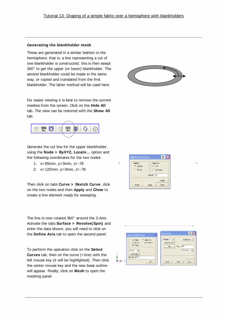
Generating the blankholder mesh

These are generated in a similar fashion to the hemisphere; that is, a line representing a cut of one blankholder is constructed; this is then swept 360° to get the upper (or lower) blankholder. The second blankholder could be made in the same way, or copied and translated from the first blankholder. The latter method will be used here.

For easier viewing it is best to remove the current meshes from the screen. Click on the Hide All tab. The view can be restored with the Show All tab.

Generate the cut line for the upper blankholder, using the Node > ByXYZ, Locate… option and the following coordinates for the two nodes:

1. x=85mm, y=0mm, z=-78 2. x=125mm, y=0mm, z=-78

Then click on tabs Curve > Sketch Curve, click on the two nodes and then Apply and Close to create a line element ready for sweeping.

The line is now rotated 360° around the Z-Axis. Activate the tabs Surface > Revolve(Spin) and enter the data shown, you will need to click on the Define Axis tab to open the second panel.

To perform the operation click on the Select Curves tab, then on the curve (=line) with the left mouse key (it will be highlighted). Then click the center mouse key and the new base outline will appear. Finally, click on Mesh to open the meshing panel.


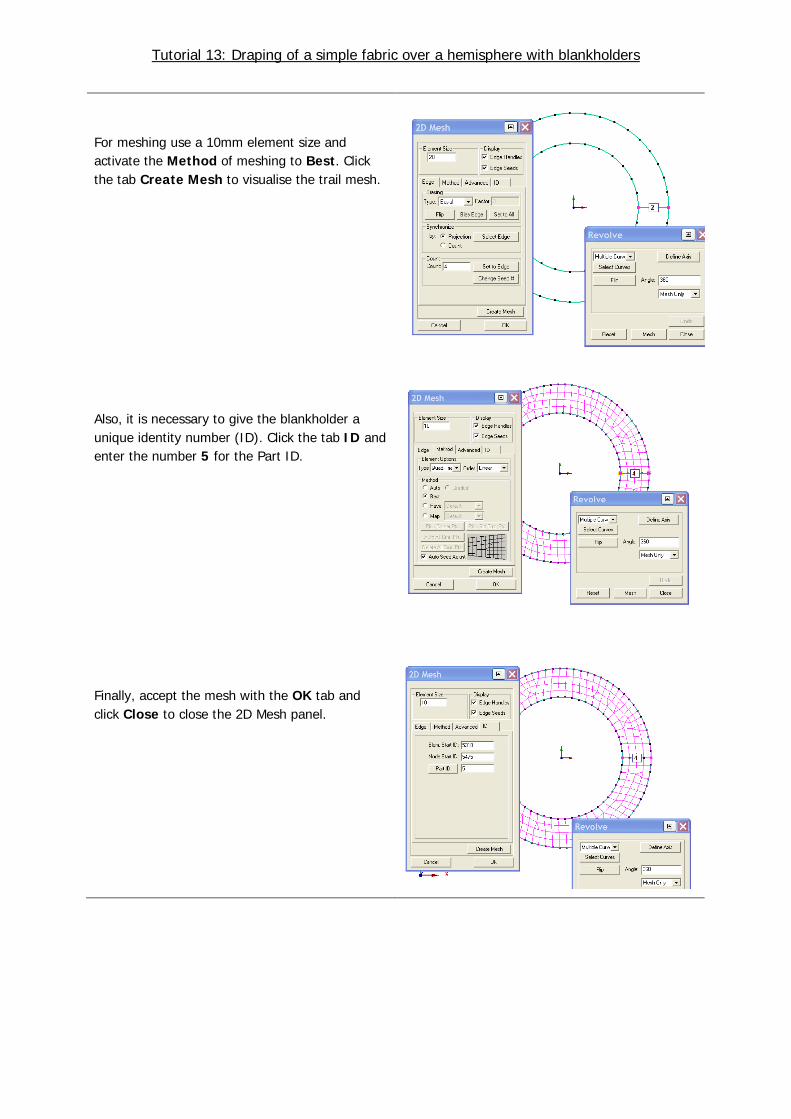
For meshing use a 10mm element size and activate the Method of meshing to Best. Click the tab Create Mesh to visualise the trail mesh.

Also, it is necessary to give the blankholder a unique identity number (ID). Click the tab ID and enter the number 5 for the Part ID.

Finally, accept the mesh with the OK tab and click Close to close the 2D Mesh panel.


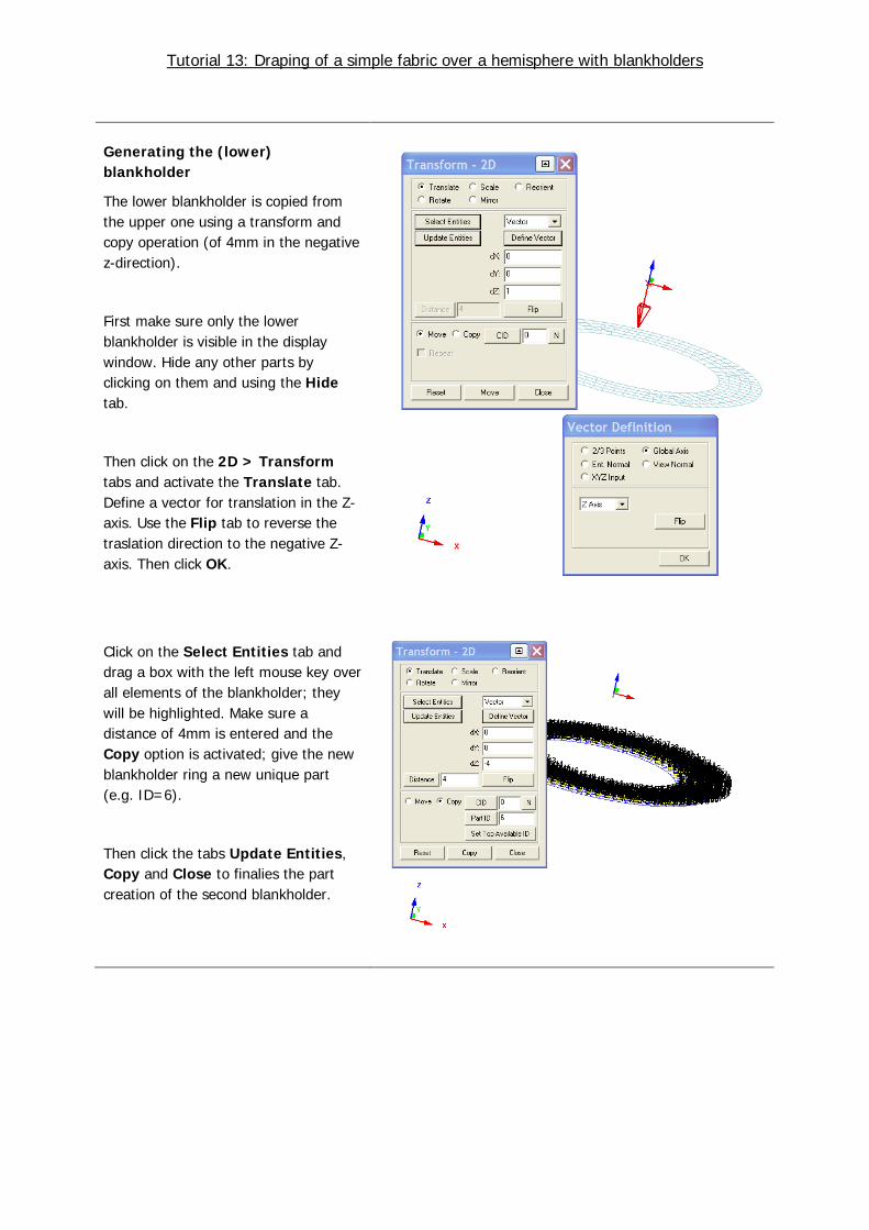
Generating the (lower) blankholder

The lower blankholder is copied from the upper one using a transform and copy operation (of 4mm in the negative z-direction).

First make sure only the lower blankholder is visible in the display window. Hide any other parts by clicking on them and using the Hide tab.

Then click on the 2D > Transform tabs and activate the Translate tab. Define a vector for translation in the Z-axis. Use the Flip tab to reverse the traslation direction to the negative Z-axis. Then click OK.

Click on the Select Entities tab and drag a box with the left mouse key over all elements of the blankholder; they will be highlighted. Make sure a distance of 4mm is entered and the Copy option is activated; give the new blankholder ring a new unique part (e.g. ID=6).

Then click the tabs Update Entities, Copy and Close to finalies the part creation of the second blankholder.


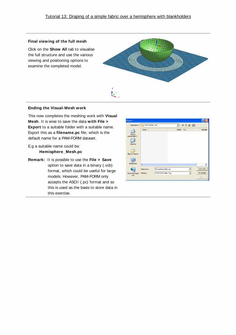
Final viewing of the full mesh

Click on the Show All tab to visualise the full structure and use the various viewing and positioning options to examine the completed model.

Ending the Visual-Mesh work

This now completes the meshing work with Visual Mesh. It is wise to save the data with File > Export to a suitable folder with a suitable name. Export this as a filename.pc file; which is the default name for a PAM-FORM dataset.

E.g a suitable name could be: Hemisphere_Mesh.pc

Remark: It is possible to use the File > Save option to save data in a binary (.vcb) format, which could be useful for large models. However, PAM-FORM only accepts the ASCII (.pc) format and so this is used as the basis to store data in this exercise.


Part 2: Defining the model data (Visual-Crash PAM)

Preparation of the model for analysis

This involves:

• Starting Visual Crash PAM for definition of entities (Loads, boundary conditions, etc.,).

• Application of constraints; the rigid body punch and blankholders will have constrained movements.

• Application of loading; the blankholders have applied pressure and the punch is velocity driven.

• Definition of part (geometric) and material properties.

• Definition of contact data and friction between blankholders, fabric and the punch.

• Definition of the PAM-FORM control data.

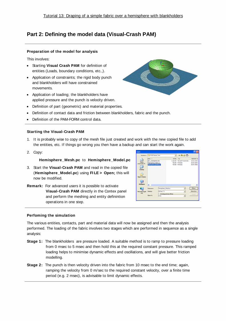
Starting the Visual-Crash PAM

1. It is probably wise to copy of the mesh file just created and work with the new copied file to add the entities, etc. If things go wrong you then have a backup and can start the work again.

2. Copy:

Hemisphere_Mesh.pc to Hemisphere_Model.pc

3. Start the Visual-Crash PAM and read in the copied file (Hemisphere_Model.pc) using FILE > Open; this will now be modified.

Remark: For advanced users it is possible to activate Visual-Crash PAM directly in the Contex panel and perform the meshing and entity definintion operations in one step.

Perfoming the simulation

The various entities, contacts, part and material data will now be assigned and then the analysis performed. The loading of the fabric involves two stages which are performed in sequence as a single analysis:

Stage 1: The blankholders are pressure loaded. A suitable method is to ramp to pressure loading from 0 msec to 5 msec and then hold this at the required constant pressure. This ramped loading helps to minimise dynamic effects and oscillations, and will give better friction modelling.

Stage 2: The punch is then velocity driven into the fabric from 10 msec to the end time; again, ramping the velocity from 0 m/sec to the required constant velocity, over a finite time period (e.g. 2 msec), is advisable to limit dynamic effects.


Constraining and (velocity) loading the punch

The punch has simple velocity loading and can be easily treated by constraining all nodes in appropriate directions and imposing a velocity time history in the Z- direction. The two steps to define the punch conditions are:

1. Constrain the punch nodes with boundary conditions by fixing all rotations and the X, Y directions.

2. Apply a velocity loading to all punch nodes in the negative Z-direction.

1. The punch boundary conditions

Click on the tabs Crash > Loads > Displacement BC to open the boundary conditions panel. In the selection type activate Part and click on the punch with the left mouse key. Then click on Update Selection to have this part number appear in the selection list. Now constrain all rotations (U,V,W) and translations (X,Y); in each case 1 means constrained, 0 means free. These are activated by clicking on each condition in the panel. Choose an appropriate title for the constraint; e.g. “punch xy fixed”. Save the selection with Apply and Close.

2. The punch applied velocity

Click on the tabs Crash > Loads > 3D BC to open the velocity BC panel; make sure the Type is set to VEL3D. In the selection type activate Part and click on the punch with the left mouse key; click on Update Selection to have this part number appear in the selection list.

1. A velocity load is applied in the Z-direction (IFUN3). Click on IFUN3 and a new panel to define the velocity curve will open. Click on NewCurve_1 and OK to define the data.

2. In the new panel define the velocity curve function. The x-axis is time and y-axis is velocity. In this case the velocity is zero to 10 msec (while the blankholders are loaded and stabilised) and then ramped to -3m/sec at 12msec. This velocity is then held constant to a time (e.g. 100msec) beyond the end simulation time (to be defined later).

3. Make sure the new velocity curve (e.g. IFUN3=1) is assigned. Close and save the selection with Apply and Close.


Application of blankholder constraints and pressure loading

For the two blankholders the following enitities and data must be a assigned:

1. Fully fix (=constrain) the lower blankholder.

2. Define the upper blankholder as a rigid body with a user defined COG node.

3. Constrain the upper blankholder COG node with appropriate boundary conditions; in this case all rotations and the X, Y directions are fixed.

4. Apply the ramped pressure loading to the upper blankholder.

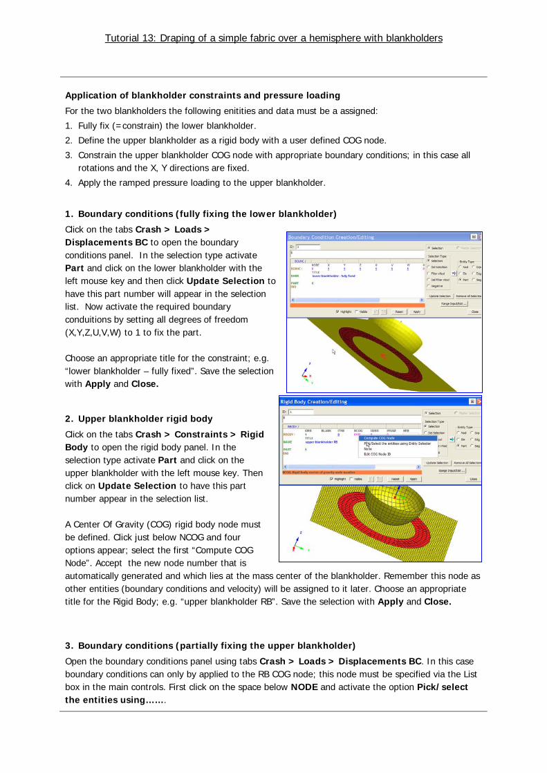
1. Boundary conditions (fully fixing the lower blankholder)

Click on the tabs Crash > Loads > Displacements BC to open the boundary conditions panel. In the selection type activate Part and click on the lower blankholder with the left mouse key and then click Update Selection to have this part number will appear in the selection list. Now activate the required boundary conduitions by setting all degrees of freedom (X,Y,Z,U,V,W) to 1 to fix the part. Choose an appropriate title for the constraint; e.g. “lower blankholder – fully fixed”. Save the selection with Apply and Close.

2. Upper blankholder rigid body

Click on the tabs Crash > Constraints > Rigid Body to open the rigid body panel. In the selection type activate Part and click on the upper blankholder with the left mouse key. Then click on Update Selection to have this part number appear in the selection list. A Center Of Gravity (COG) rigid body node must be defined. Click just below NCOG and four options appear; select the first “Compute COG Node”. Accept the new node number that is automatically generated and which lies at the mass center of the blankholder. Remember this node as other entities (boundary conditions and velocity) will be assigned to it later. Choose an appropriate title for the Rigid Body; e.g. “upper blankholder RB”. Save the selection with Apply and Close.

3. Boundary conditions (partially fixing the upper blankholder)

Open the boundary conditions panel using tabs Crash > Loads > Displacements BC. In this case boundary conditions can only by applied to the RB COG node; this node must be specified via the List box in the main controls. First click on the space below NODE and activate the option Pick/select the entities using…….


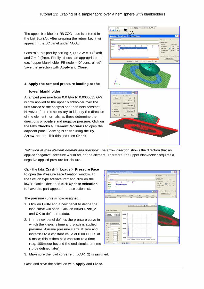
(A)

The upper blankholder RB COG node is entered in the List Box (A). After pressing the return key it will appear in the BC panel under NODE. Constrain this part by setting X,Y,U,V,W = 1 (fixed) and Z = 0 (free). Finally, choose an appropriate title e.g. “upper blankholder RB node – XY constrained”. Save the selection with Apply and Close.

4. Apply the ramped pressure loading to the

lower blankholder

A ramped pressure from 0.0 GPa to 0.0000035 GPa is now applied to the upper blankholder over the first 5msec of the analysis and then held constant. However, first it is necessary to identify the direction of the element normals, as these determine the directions of positive and negative pressure. Click on the tabs Checks > Element Normals to open the adjacent panel. Viewing is easier using the By Arrow option; click this and then Check. Definition of shell element normals and pressure: The arrow direction shows the direction that an applied “negative” pressure would act on the element. Therefore, the upper blankholder requires a negative applied pressure for closure. Click the tabs Crash > Loads > Pressure Face to open the Pressure Face Creation window. In the Section type activate Part and click on the lower blankholder; then click Update selection to have this part appear in the selection list. The pressure curve is now assigned:

1. Click on IFUN and a new panel to define the load curve will open. Click on NewCurve_2 and OK to define the data.

2. In the new panel defines the pressure curve in which the x-axis is time and y-axis is applied pressure. Assume pressure starts at zero and increases to a constant value of 0.00000355 at 5 msec; this is then held constant to a time (e.g. 100msec) beyond the end simulation time (to be defined later).

3. Make sure the load curve (e.g. LCUR=2) is assigned. Close and save the selection with Apply and Close.


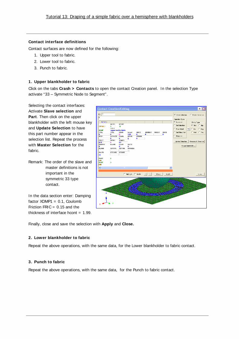
Contact interface definitions

Contact surfaces are now defined for the following:

1. Upper tool to fabric.

2. Lower tool to fabric.

3. Punch to fabric.

1. Upper blankholder to fabric

Click on the tabs Crash > Contacts to open the contact Creation panel. In the selection Type activate “33 – Symmetric Node to Segment”. Selecting the contact interfaces: Activate Slave selection and Part. Then click on the upper blankholder with the left mouse key and Update Selection to have this part number appear in the selection list. Repeat the process with Master Selection for the fabric. Remark: The order of the slave and

master definitions is not important in the symmetric 33 type contact.

In the data section enter: Damping factor XDMP1 = 0.1, Coulomb Friction FRIC = 0.15 and the thickness of interface hcont = 1.99. Finally, close and save the selection with Apply and Close.

2. Lower blankholder to fabric

Repeat the above operations, with the same data, for the Lower blankholder to fabric contact.

3. Punch to fabric

Repeat the above operations, with the same data, for the Punch to fabric contact.


Assigning the Material and Part data

This is done using two entities which are linked together; namely: 1. The Material data for material data such as density, fibre modulus and resin viscosity. 2. The Part data for geometric data such as thickness and fibre angles. Material models: • Rigid tooling: In this example the tools (blankholders and punch) are both effectively rigid and can

therefore be modelled using the 100-Null shell element material model. This model requires some material properties which are only used to determine contact penalty forces.

• Fabric: This is modelled using the fabric specific material model 140. •

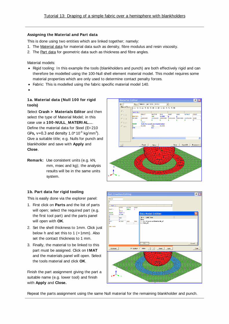
1a. Material data (Null 100 for rigid tools)

Select Crash > Materials Editor and then select the type of Material Model; in this case use a 100-NULL_MATERIAL…. Define the material data for Steel (E=210 GPa, ν=0.3 and density 1.0*10-6 kg/mm3). Give a suitable title; e.g. Nulls for punch and blankholder and save with Apply and Close. Remark: Use consistent units (e.g. kN,

mm, msec and kg); the analysis results will be in the same units system.

1b. Part data for rigid tooling

This is easily done via the explorer panel:

1. First click on Parts and the list of parts will open; select the required part (e.g. the first tool part) and the parts panel will open with OK.

2. Set the shell thickness to 1mm. Click just below h and set this to 1 (=1mm). Also set the contact thickness to 1 mm.

3. Finally, the material to be linked to this part must be assigned. Click on IMAT and the materials panel will open. Select the tools material and click OK.

Finish the part assignment giving the part a suitable name (e.g. lower tool) and finish with Apply and Close. Repeat the parts assignment using the same Null material for the remaining blankholder and punch.


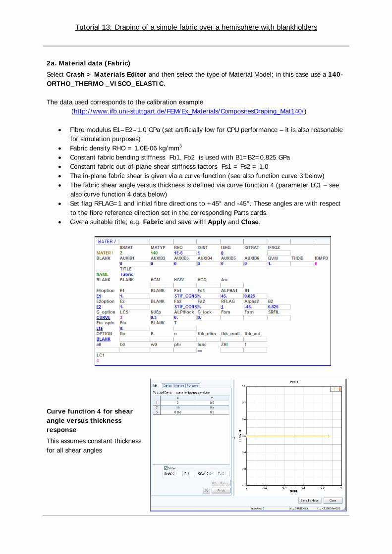
2a. Material data (Fabric)

Select Crash > Materials Editor and then select the type of Material Model; in this case use a 140-ORTHO_THERMO _VISCO_ELASTIC. The data used corresponds to the calibration example (http://www.ifb.uni-stuttgart.de/FEM/Ex_Materials/CompositesDraping_Mat140/)

• Fibre modulus E1=E2=1.0 GPa (set artificially low for CPU performance – it is also reasonable for simulation purposes)

• Fabric density RHO = 1.0E-06 kg/mm3 • Constant fabric bending stiffness Fb1, Fb2 is used with B1=B2=0.825 GPa • Constant fabric out-of-plane shear stiffness factors Fs1 = Fs2 = 1.0 • The in-plane fabric shear is given via a curve function (see also function curve 3 below) • The fabric shear angle versus thickness is defined via curve function 4 (parameter LC1 – see

also curve function 4 data below) • Set flag RFLAG=1 and initial fibre directions to +45° and -45°. These angles are with respect

to the fibre reference direction set in the corresponding Parts cards. • Give a suitable title; e.g. Fabric and save with Apply and Close.

Curve function 4 for shear angle versus thickness response

This assumes constant thickness for all shear angles

http://www.ifb.uni-stuttgart.de/FEM/Ex_Materials/CompositesDraping_Mat140/�


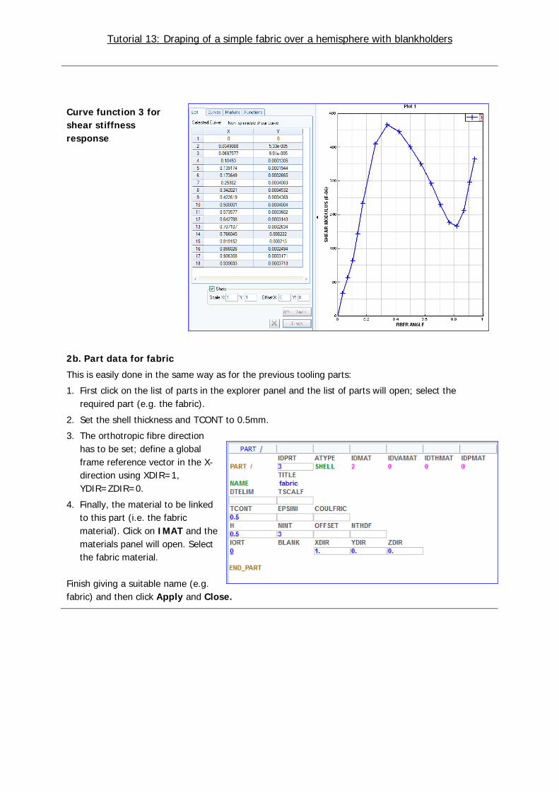
Curve function 3 for shear stiffness response

2b. Part data for fabric

This is easily done in the same way as for the previous tooling parts:

1. First click on the list of parts in the explorer panel and the list of parts will open; select the required part (e.g. the fabric).

2. Set the shell thickness and TCONT to 0.5mm.

3. The orthotropic fibre direction has to be set; define a global frame reference vector in the X-direction using XDIR=1, YDIR=ZDIR=0.

4. Finally, the material to be linked to this part (i.e. the fabric material). Click on IMAT and the materials panel will open. Select the fabric material.

Finish giving a suitable name (e.g. fabric) and then click Apply and Close.


Output results

If detailed element data is to be studied these should be placed in the element time histories for data storage on the results files.

Click Crash > Output > Element TH and activate selection type Ele. Then select several elements in the fabric (click on them using the left mouse key). Click on Update Selection to have these appear on the output selection. Finally give a suitable title (e.g. selected elements) and finish with Apply and Close.

Defining some basic model data

For the PAM-FORM controls set the following parameters: INPUT- VERSION

Set the PAM-CRASH version being used (e.g. 2012)

RUNEND Termination time for the analysis (=35.0 msec)

SOLVER Use STAMP for a PAM-FORM analysis (This still uses the PAM-CRASH code with special options and outputs)

OCTRL

• THPOUTPUT – output interval for graphical (x,y) time history information (e.g. use POINTS = 1000 for one thousand points)

• DSYOUTPUT - output interval for deformed states (e.g. use INTERVAL = 1.0 for a picture output at every 1msec)

• Parameter ERFOUTPUT - for a .erfh5 results file specify type 3 without compression (ICOMPRES=0)

TITLE An optional title for output plots/results can be defined

ANALYSIS Use EXPLICIT for a dynamic analysis

Saving the dataset

Save (update) the dataset Hemisphere_Model.pc using the File > Export option.

A C

B


Part 2: Explicit analysis of the Hemisphere draping problem The PAM-FORM dataset is run (using PAM-FORM or PAM-CRASH with special license options). The results files generated are:

• Hemisphere_Model.THP for x-y time history plot information at selected points, elements, etc.

• Hemisphere_Model.DSY for deformation and contour plots of the full model.

In version V2012 the Hemisphere_Model_RESULT.erfh5 file is also output containing both information types. However, this is still under development (January 2013) and does not contain all forming information; consequently, the .THP and .DSY files are used here.

Evaluating the results (Visual Viewer) First, we shall look at selected results of the deformed structure and some information that are available for contour plots of the complete structure; these are stored in the .DSY file at specified time intervals (states).

Start Visual Viewer and open the Hemisphere_Model.DSY file.

1. Click Results > Animation Control and you will be able to visualise the model and use the adjacent panel to examine deformations, either at a certain time, or as an animation.

Use the Speed Control option to change the viewing speed. Additional tabs are available for overlaying the Initial Mesh or Simultaneous Display of selected states.

Click Close to exit this option.

2. It can be useful to remove parts from the viewing; for example the punch and blank-holder that hide the fabric. Or transparency can be applied to certain parts. For this Parts Viewing in the Explorer window is activated and options selected.


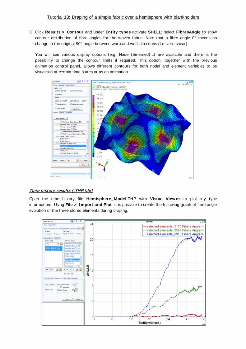
3. Click Results > Contour and under Entity types activate SHELL; select FibresAngle to show contour distribution of fibre angles for the woven fabric. Note that a fibre angle 0° means no change in the original 90° angle between warp and weft directions (i.e. zero shear).

You will see various display options (e.g. Node (Smeared)…) are available and there is the possibility to change the contour limits if required. This option, together with the previous animation control panel, allows different contours for both nodal and element variables to be visualised at certain time states or as an animation.

Time history results (.THP file)

Open the time history file Hemisphere_Model.THP with Visual Viewer to plot x-y type information. Using File > Import and Plot it is possible to create the following graph of fibre angle evolution of the three stored elements during draping.


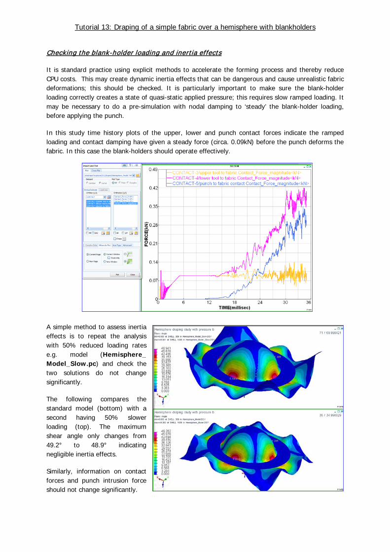
Checking the blank-holder loading and inertia effects

It is standard practice using explicit methods to accelerate the forming process and thereby reduce CPU costs. This may create dynamic inertia effects that can be dangerous and cause unrealistic fabric deformations; this should be checked. It is particularly important to make sure the blank-holder loading correctly creates a state of quasi-static applied pressure; this requires slow ramped loading. It may be necessary to do a pre-simulation with nodal damping to ‘steady’ the blank-holder loading, before applying the punch.

In this study time history plots of the upper, lower and punch contact forces indicate the ramped loading and contact damping have given a steady force (circa. 0.09kN) before the punch deforms the fabric. In this case the blank-holders should operate effectively.

A simple method to assess inertia effects is to repeat the analysis with 50% reduced loading rates e.g. model (Hemisphere_ Model_Slow.pc) and check the two solutions do not change significantly.

The following compares the standard model (bottom) with a second having 50% slower loading (top). The maximum shear angle only changes from 49.2° to 48.9° indicating negligible inertia effects.

Similarly, information on contact forces and punch intrusion force should not change significantly.

Exercise 1 – table under static loading€¦ · exercise and the tutorial is valid. Preparing the...

Documents

Transcript of Exercise 1 – table under static loading€¦ · exercise and the tutorial is valid. Preparing the...