Executive Summary - North Pacific Fishery … · Web viewF8 where p LnF GTF is a parameter...

Potential Revisions to the Tanner Crab Stock Assessment Model and Input Data for the 2014 Stock Assessment and Fishery Evaluation Report for the Tanner

Crab Fisheries of the Bering Sea and Aleutian Islands Regions

William T. StockhausenAlaska Fisheries Science Center

April 2014

THIS INFORMATION IS DISTRIBUTED SOLELY FOR THE PURPOSE OF PREDISSEMINATION PEER REVIEW UNDER APPLICABLE INFORMATION QUALITY GUIDELINES. IT HAS NOT BEEN FORMALLY DISSEMINATED BY NOAA

FISHERIES/ALASKA FISHERIES SCIENCE CENTER AND SHOULD NOT BE CONSTRUED TO REPRESENT ANY AGENCY DETERMINATION OR POLICY

Executive Summary1. Stock: species/area.Southern Tanner crab (Chionoecetes bairdi) in the eastern Bering Sea (EBS).

2. Catches: trends and current levels.Legal-sized male Tanner crab are caught and retained in the directed (male-only) Tanner crab fishery in the EBS. The directed fishery was closed most recently by the State of Alaska (SOA) during the 2010/11, 2011/12, and 2012/13 fishing years (July 1-June 30) because estimated female stock metrics did not meet the required threshold in the state harvest strategy. In 2013/14, the SOA opened the directed fishery with Total Allowable Catches (TACs) of 1,645,000 lbs (746 t) in the Western Region and 1,463,000 lbs (664 t) in the Eastern Region. The fishery concluded on March 31, 2014. Preliminary results indicate that 80.9% (604 t) of the TAC was harvested in the Western Region and 99.5% (661 t) was taken in the Eastern Region (M. Good, pers. comm.). Fourteen vessels participated in the Western Region fishery, while 18 participated in the Eastern Region fishery.

3. Stock biomass: trends and current levels relative to virgin or historic levelsModel-estimated MMB in 2012/13 was 59.4 thousand t (Stockhausen et al. 2013), essentially unchanged from that in 2011/12 (59.3 thousand t). MMB has undergone a slight downward trend since its most recent peak in 2009/10 but it remains above the very low levels seen in the mid-1990s to early 2000s (1990 to 2005 average: 31.5 thousand t). However, it is considerably below historic levels in the early 1970s when MMB peaked at 352.5 thousand t (1972/73).

4. Recruitment: trends and current levels relative to virgin or historic levels.Estimated male recruitment in 2013/14 (number of crab entering the population on July 1) was 120,593 thousand crab (Stockhausen et al. 2013). This represents a 2.6-fold increase over that in 2012/13 (33,758 thousand crab), but a 5.9 decrease over that in 2011/12 (128,170 thousand crab). It was also smaller than those occurring in 2009/10 and 2010/11, but larger than those occurring in 2005/06-2008/09. Going back to 1990/91, the 2013/14 estimated male recruitment ranked the 6th largest (out of 24 years). However, the estimated 2013/14 male recruitment is substantially smaller than those occurring from the early-1960s to 1990, which averaged 317,073 thousand crab.

1

5. Management performance

(a) Historical status and catch specifications (millions lb) for eastern Bering Sea Tanner crab (Stockhausen et al. 2013).

Year MSSTBiomass (MMB)

TAC (East + West)

Retained Catch

Total Catch

Mortality OFL ABC

2009/10 92.37B 62.70B 1.34a/ 1.32 3.62 5.00A

2010/11 91.87C 58.93C 0.00 0.00 1.92 3.20B

2011/12 25.13D 129.17D 0.00 0.00 2.73 6.06C 5.47 C

2012/13 36.97E 130.84E 0.00 0.00 1.57 41.93D 18.01D

2013/14 TBD 117.07E 3.11 2.79 F TBD 55.89E 39.29E

(b) Historical status and catch specifications (thousands t) for eastern Bering Sea Tanner crab (Stockhausen et al. 2013).

Year MSSTBiomass (MMB)

TAC (East + West)

Retained Catch

Total Catch

Mortality OFL ABC

2009/10 41.90B 28.44B 0.61a/ 0.6 1.64 2.27A

2010/11 41.67C 26.73C 0 0 0.87 1.45B

2011/12 11.40D 58.59D 0 0 1.24 2.75C 2.48C

2012/13 16.77E 59.35E 0 0 0.71 19.02D 8.17D

2013/14 TBD 53.1E 1.41 1,265F TBD 25.35E 17.82E

a/ Only the area east of 166o W opened in 2009/10.A—Calculated from the assessment reviewed by the Crab Plan Team in 2009.B—Calculated from the assessment reviewed by the Crab Plan Team in 2010.C—Calculated from the assessment reviewed by the Crab Plan Team in 2011.D—Calculated from the assessment reviewed by the Crab Plan Team in 2012.E—Calculated from the assessment reviewed by the Crab Plan Team in 2013.F—Preliminary estimates.

2

6. Basis for the OFL

Basis for the OFL (thousands t) (Stockhausen et al. 2013).

Year Tier BMSY

Current MMB

B/BMSY

(MMB) FOFL

Years to define BMSY

Natural Mortality

2012/13A 3a 33.45 59.35 1.75 0.61 yr-1 1982-2012 0.23 yr-1 B

2013/14C 3a 33.54 53.1 1.77 0.73 yr-1 1982-2013 0.23 yr-1 D

A—Calculated from the assessment reviewed by the Crab Plan Team in 2012.B—Nominal rate of natural mortality. Actual rates used in the 2012 assessment were 0.25 yr -1 for immature females and all males

and 0.34 yr-1 for mature females.C— Calculated from the assessment reviewed by the Crab Plan Team in 2013.D—Nominal rate of natural mortality. Actual rates used in the 2013 assessment were 0.25 yr -1 for immature females and all males

and 0.34 yr-1 for mature females.

Current male spawning stock biomass (MMB) is estimated at 53.1 thousand t. BMSY for this stock is calculated to be 33.54 thousand t, so MSST is 16.77. Because current MMB > MSST, the stock is not overfished. Total catch mortality (retained + discard mortality in all fisheries) in 2012/13 was 0.71 thousand t, which was less than the OFL for 2012/13 (19.02 thousand t); consequently overfishing did not occur.

7. Rebuilding analyses summary.The EBS Tanner crab stock was found to be above MSST (and BMSY) in the 2012 assessment (Rugolo and Turnock, 2012) and was subsequently declared rebuilt. Consequently no rebuilding analyses were conducted (Stockhausen et al. 2013).

Summary of Major Changes1. Changes (if any) to the management of the fishery.Based on a newly-accepted assessment model (Rugolo and Turnock, 2012), the Science and Statistical Committee (SSC) of the North Pacific Fisheries Management Council (NPFMC) moved the Tanner crab stock from Tier 4 to Tier 3 for status determination and OFL setting in October 2012. Status determination and OFL setting for Tier 4 stocks generally depends on current survey biomass and a proxy for BMSY based on survey biomass averaged over a specified time period. In Tier 3, status determination and OFL setting depend on a model-estimated value for current MMB at mating time as well as proxies for FMSY and BMSY based on spawning biomass-per-recruit calculations and average recruitment to the population over a specified time period. The change from Tier 4 to Tier 3 resulted in a large reduction in the BMSY used for status determination from 83.33 thousand t in 2011 to 33.45 thousand t in 2012. Concurrently, the estimated assessment-year MMB increased from 26.73 thousand t in 2011 to 58.59 thousand t in 2012. As a consequence, the status of Tanner crab changed from being an overfished stock following the 2011 assessment to one that was not-overfished following the 2012 assessment. The stock was subsequently declared rebuilt and an OFL of 19.02 thousand t was set for 2012/13.

Although the stock was declared rebuilt as a result of the 2012 assessment, the directed fishery for Tanner crab remained closed by the SOA on the basis of its algorithms for setting harvest levels. As a result of the 2013 assessment (Stockhausen et al., 2013), however, the SOA re-opened the directed fishery for 2013/14. TACs of 746 t (1,645,000 lbs) and 664 t (1,463,000 lbs) were set in the Western and Eastern Regions (Fig. 1), respectively. The fishery concluded on March 31, 2014. Preliminary results indicate that 80.9% (604 t) of the TAC was harvested in the Western Region and 99.5% (661 t) was taken in the Eastern Region (M. Good, pers. comm.).

3

2. Changes to the input dataA number of potential changes to the input data used for the 2013 assessment model are considered here as a series of discrete changes (Table 1) The first of these (dataset B; Table 1) corrects several errors in the 2013 assessment data that were found after the assessment was completed. These include errors copying the size frequencies used for immature, new shell females from the 2013 AFSC trawl survey and the sample sizes assigned to the sex-specific bycatch size frequencies from the groundfish fisheries from the original files to those used by the assessment model. The remaining changes (datasets C-E) incorporate changes to size frequency information from the various crab fisheries and the groundfish fisheries following requests by the CPT to recalculate the dockside (retained) and at-sea observer-based size frequencies in the crab fisheries (W. Gaeuman) and the at-sea observer-based bycatch size frequencies in the groundfish fisheries (R. Foy).

3. Changes to the assessment methodology.Two models, referred to as TCSAM2013and TCSAM2013Rev, are compared here using datasets A and E mentioned above. TCSAM2013 is the model that was used to conduct the 2013 assessment (see Appendix 1 for a detailed description of this model). TCSAM2013 directly estimates size-specific total (retained+discard) fishing mortality rates from the input data for male crab in the directed fishery and assumed discard mortality rates. It derives size-specific retained mortality rates on males from a combination of the size-specific total fishing mortality rates and an additional “retention curve” that is assumed to reflect the on-deck sorting process. However, this is not logically consistent. This logical inconsistency is discussed more fully in Appendix 2, which provides a complete derivation of the fishing mortality equations that should be used for a fished stock caught in multiple fisheries, in which partial survival of discarded bycatch occurs.

The second model, TCSAM2013Rev, uses the fishing mortality equations developed in Appendix 2 and corrects the logical inconsistency in TCSAM2013 by reformulating total fishing mortality and retained mortality rates in terms of total fishing capture rates (i.e., the rates at which crab are brought on board, not the rates at which they are killed—which are derived quantities; see Appendix 2). Otherwise, TCSAM2013Rev is identical to TCSAM2013 (only a few lines of code were required to be changed to achieve this revision).

A description of TCSAM2014, a third model that is currently under development, is also provided (Appendix 3). TCSAM2014 represents a complete revision of the TCSAM2013 model code and incorporates the changes to modeling fishing mortality contained in TCSAM2013Rev. The new code eliminates everything that was hard-wired in the old code. It provides a much more flexible assessment model (in terms of data inputs, model parameter specification, temporal regime definitions, and fishery and survey specifications). It also provides the ability to address SSC requests such as retrospective analyses in a much simpler, less time-consuming fashion than was possible with the old code.

4

IntroductionThis report addresses two issues in the Tanner crab stock assessment that have arisen subsequent to the Fall 2013 assessment. It also provides a description of a new assessment model under development.

The first issue regards the datasets used in the stock assessment. Following a discussion at the 2014 Crab Modeling Workshop (Crab Plan Team, 2014), the Crab Plan Team (CPT) recognized that many crab assessments included “‘legacy’ data, the origins of which are uncertain”, partly as a result of changes in analysts over time and partly a result of the length of some of the data time series. The CPT requested that W. Gaeuman (ADFG) provide assessment authors with updated information on crab fishery discards (total numbers discarded and length frequencies for discards and total observed catch). This new information is reviewed here and changes to assessment model results are evaluated. In addition to the new information from W. Gaeuman, two other changes to the input data to the Tanner crab assessment are also evaluated. The first change addresses the correction of two inadvertent errors in the dataset used in the 2013 Tanner crab assessment, while the second incorporates updated information on bycatch size frequencies of Tanner crab in the groundfish fisheries provided to the author by R. Foy (NMFS/AFSC).

The second issue concerns a logical inconsistency in the manner in which fishing mortality is described in the 2013 stock assessment model (hereafter referred to as TCSAM2013).As part of an effort to improve the assessment, I wrote a new description of the Tanner crab model used in the 2013 assessment (TCSAM2013; Appendix 1). In the course of writing the new description, I realized that the equations used to describe total fishing mortality and retained mortality did not seem consistent with those used in Gmacs (Generalized Modeling for Alaskan Crab Stocks), a generic modeling framework for crab assessments being developed by A. Whitten, J. Ianelli and A. Punt (Whitten et al., 2013). To resolve this, I derived a set of equations describing fishing mortality on crab stocks from first principles (Appendix 2). The resulting equations are the same that are used in Gmacs and differ from those in TCSAM2013. I consequently revised the TCSAM2013 code to reflect the corrected equations (TCSAM2013Rev) and compare results from the two models using the 2013 assessment dataset and the dataset that incorporates all the corrections and updates referred to previously.

Finally, this report includes a description of a new version of the Tanner crab assessment model, TCSAM2014, which is under development and will be available for use in the 2014 assessment. Although eventually a Gmacs-based Tanner crab model will developed, the time frame for such a model is somewhat uncertain and an intermediate model is required. TCSAM2014 represents a complete revision of the TCSAM2013 model code and incorporates the changes to modeling fishing mortality contained in TCSAM2013Rev. The new code eliminates everything that was hard-wired in the old code. It provides a much more flexible assessment model (in terms of data inputs, model parameter specification, temporal regime definitions, and fishery and survey specifications). It also provides the ability to address SSC requests such as retrospective analyses in a much simpler, less time-consuming fashion than was possible with the old code.

Data Revisions

Revisions to the dataFour revisions to the data used in the 2013 Tanner crab assessment are considered in this report (Table 1). The impact of these changes on results from the 2013 assessment model are evaluated in a stepwise, cumulative fashion. Data revision B corrects two errors in the 2013 assessment data (dataset A) that were detected after the 2013 assessment had been completed. In the first of these errors, the size frequency for immature, new shell females from the 2013 AFSC trawl survey was incorrectly copied into the model data file. The corrected version shows two peaks in the size frequency (in the 27.5 and 62.5 mm CW size bins) of similar size, while the version used in the assessment is more reflective of a single peak in the

5

smallest size bin (27.5 mm CW) (Fig. 2). In the second error, the sex-specific sample sizes (Fig. 3) for bycatch size frequencies in the groundfish fisheries had been inadvertently switched between males and females. This error appears to have been introduced prior to the 2012 assessment.

Data revision C incorporates retained size frequencies from dockside observer sampling for male crabs by shell condition in the directed Tanner crab fishery from 1991-2009 as recalculated by W. Gaeuman and provided to the author (Table 2, Fig.s 4 and 5). Dataset C does not include size frequencies for 1995, although these were included in the assessment, because the numbers of individuals sampled were relatively small. Comparing the new data with the old, all years agree in terms of the number of measured crab (Table 2, Figure 4) except for new shell males in 2008 (429 fewer crab were included in the recalculated dataset) and both shell conditions in 2009 (almost 12,000 fewer crab were included in the recalculated dataset. The differences in the resulting size frequencies appear small for the new shell males but rather substantial for the 2009 old shell males. The reason(s) for the rather large discrepancies in total numbers sampled for 2008 and 2009 is unknown, but should be identified, if possible.

Data revision D incorporates total catch size frequencies for Tanner crab from at-sea observer sampling in the crab fisheries starting in 1990 as recalculated by W. Gaeuman and provided to the author (Tables 3-5, Fig.s 6-8). The numbers of crab sampled are substantially different in the recalculated and assessment datasets in some circumstances (e.g., ~40,000 males for 1992 in the directed fishery, Table 3) but are identical in others (e.g. 5,972 males in both datasets for 1994 in the directed fishery, Table 3). Once again, the reason(s) for these large discrepancies is currently unknown but should be identified if possible.

Data revision E incorporates bycatch size frequencies for Tanner crab in the groundfish fisheries from at-sea observer sampling starting in 1973 from data files provided by R. Foy that he extracted from AFSC’s Groundfish Observer Program database. The numbers of crab sampled are again substantially different between the recalculated and assessment datasets (Table 6, Fig. 9). However, two sources for the differences are known. The first is that the recalculated dataset includes observer sampling from the joint venture fisheries in the late 1980s while the dataset used in the assessment does not. The second is that the recalculated dataset bases the size frequencies on the crab fishery year (July 1-June30) while the assessment dataset used the groundfish fishery year (Jan. 1-Dec. 31).

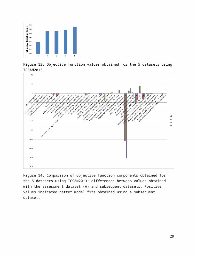
Impacts on assessment resultsAssessing the impacts of the data revisions on the assessment was addressed by running the model used in the 2013 assessment (TCSAM2013) on each of the datasets and comparing model results for changes to the time series of estimated mature male biomass (MMB) at mating (Fig. 10), recruitment (Fig. 11), fully-selected fishing mortality in the directed fishery (Fig. 12), and changes to the different components comprising the model objective function (Fig.s 13 and 14). The resulting changes in the assessment model output are reasonably small across the time series for MMB, recruitment and directed fishing mortality. Correcting the errors to the assessment dataset (data revision B) resulted in a 12% increase in final (2012) MMB as well as 4% higher average recruitment (1982-2013), although the estimated final recruitment decreased (consistent with the correction to the 2013 trawl survey size frequency for immature, new shell females). Subsequent changes to the various size frequencies incorporated in the model data (revisions C-E) had smaller impacts on the model estimates in the terminal year of each time series.

Interestingly, the data revisions resulted in increasingly worse fits by the model (reflected by increasing values of the objective function for each data revision; Fig. 13). The correction to the sample sizes used for male and female bycatch size frequencies in the groundfish fisheries resulted in a large increase in the mis-fit of the model to the data. This may indicate that the total bycatch biomass time series needs to be revised, as well, because only the size frequencies were changed, not the total numbers or biomass for discards.

6

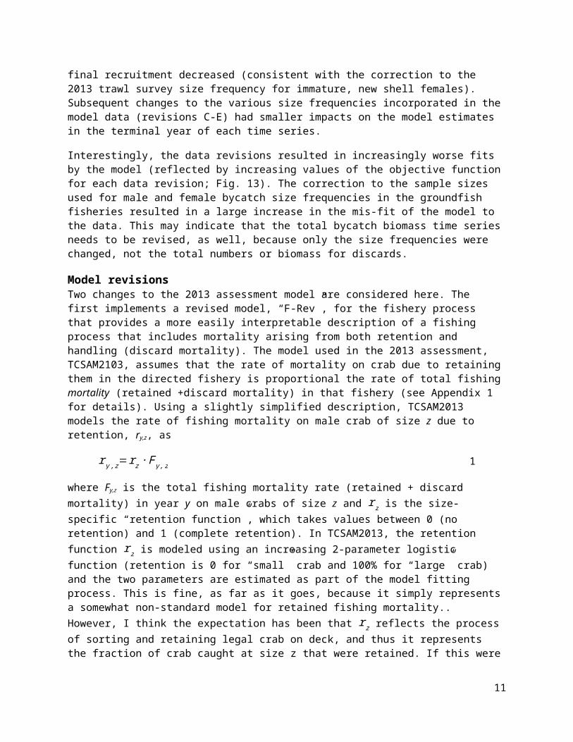
Model revisionsTwo changes to the 2013 assessment model are considered here. The first implements a revised model, “F-Rev”, for the fishery process that provides a more easily interpretable description of a fishing process that includes mortality arising from both retention and handling (discard mortality). The model used in the 2013 assessment, TCSAM2103, assumes that the rate of mortality on crab due to retaining them in the directed fishery is proportional the rate of total fishing mortality (retained +discard mortality) in that fishery (see Appendix 1 for details). Using a slightly simplified description, TCSAM2013 models the rate of fishing mortality on male crab of size z due to retention, ry,z, as

r y, z=r z∙ F y, z 1

where Fy,z is the total fishing mortality rate (retained + discard mortality) in year y on male crabs of size z and r z is the size-specific “retention function”, which takes values between 0 (no retention) and 1 (complete retention). In TCSAM2013, the retention function r z is modeled using an increasing 2-parameter logistic function (retention is 0 for “small” crab and 100% for “large” crab) and the two parameters are estimated as part of the model fitting process. This is fine, as far as it goes, because it simply represents a somewhat non-standard model for retained fishing mortality.. However, I think the expectation has been that r z reflects the process of sorting and retaining legal crab on deck, and thus it represents the fraction of crab caught at size z that were retained. If this were the case, r z would be independent of handling mortality because what’s retained is not affected by what’s discarded (rather it’s the other way around: what’s discarded is simply wjhat’s left over after crab to be retained have been selected). However, this is not the correct interpretation of r z as it is used in TCSAM2013 and eq. 1 above. Rather, r z in eq. 1 simply reflects the fraction of crab killed at size z that were killed because they were retained, as opposed to being killed as part of the discard process. As such, it is actually a function of the assumed handling mortality on discarded crab whereas the function that describes the on-deck sorting process is not. As an illustration to make this point, if handling mortality were 0 then all fishing mortality F y , z would be due to retention (r y, z=F y, z) and r z would be identically 1 irrespective of any sorting process that occurred on deck (e.g., all sub-legals being discarded).

The revised model for the fishing process used in F-Rev is developed in detail in Appendix 2. It models the size-specific fishing mortality rate in the directed fishery using

F y , z=(h∙ [1−ρ z ]+ρ z ) ∙ ϕ y , z 2

where h is handling mortality, ρ z is the size-specific “retention function” that reflects the on-board sorting process, and ϕ y , z is the fishery capture rate for crab of size z in year y. In this formulation, ϕ y , z reflects the rate at which crab are brought on deck, ρ z is the fraction of crab captured (not killed) that are retained (and thus die), and h is the fraction of discarded crab ([1−ρz ]) that die due to handling. The equation that describes the fishing mortality rate due to retention, the equivalent to eq. 1, is simply

r y, z=ρ z ∙ ϕ y , z 3

The fishery capture rate ϕ y , z in the revised model is treated with the same assumptions that F y , z is treated with in TCSAM2013: it is modeled as a separable function of size and year

ϕ y , z=ϕ y ∙ Sz 4

7

where ϕ y is the “fully-selected” capture rate in year y and Sz is the size-specific capture selectivity. ϕ y is parameterized in a similar fashion to the fully-selected fishing mortality rate Fy in TCSAM2013. The capture selectivity S z and retention function ρ z are also parameterized in the same way as selectivity and the retention function rz in TCSAM2013.

The second change to TCSAM2013 “turns on” estimation of fishing mortality parameters associated with bycatch of Tanner crab in the BBRKC fishery in the 1992-2012 time period. These had been turned off in the 2012 assessment to improve model convergence and the issue was not re-examined in the 2013 assessment. In the course of testing the revision to the fishing mortality model, I also revisited this issue.

The model changes were evaluated in an orthogonal manner using Datasets A (the data used in the 2013 assessment) and E (incorporating all data revisions considered in the previous section; Table 1). Thus, results from the 2013 assessment model (“Base”) using Datasets A and E were compared with models run using the same two datasets but incorporating 1) the F-Rev capture rate model (but otherwise identical to TCSAM2013), 2) estimating the BBRKC fishing mortality parameters for 1992-2012 (“RKF est”), and 3) the two changes combined (“F-Rev+RKF est”).

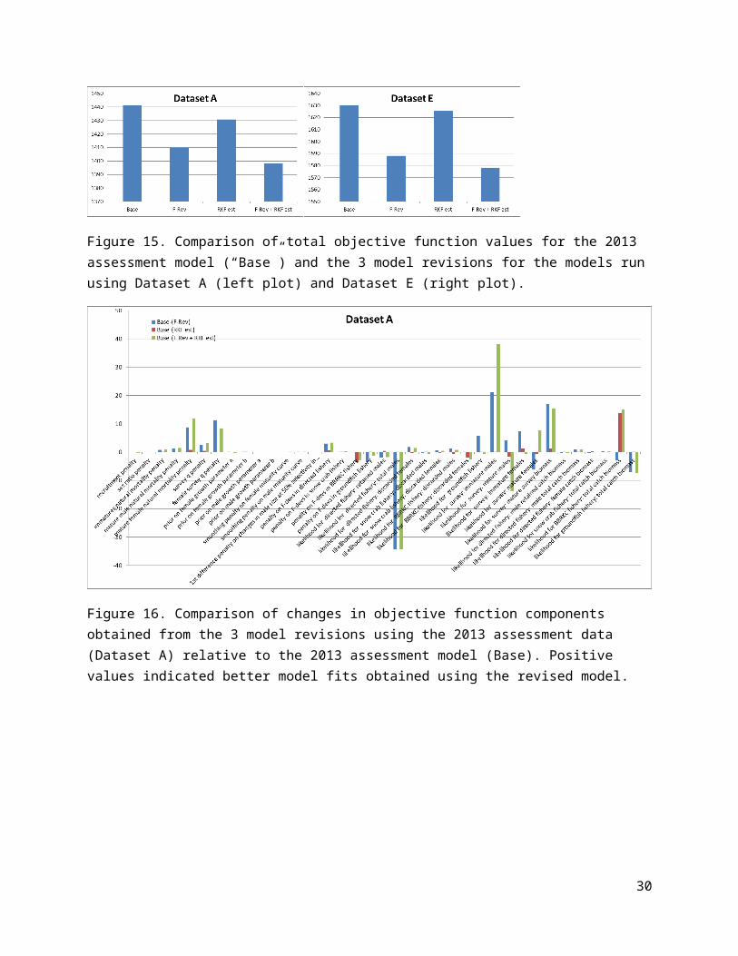
Impacts on assessment resultsBased on the objective function value at model convergence for each of the models, using the revised fishing mortality model improved the overall model fit by about 30 units over the base (2013 assessment) model using the assessment data (Dataset A) and about 40 units using Dataset E (Fig. 15). Estimating the BBRKC fishing mortality parameters improved the fit by about 10 units over the base model using Dataset A but only 5 units using Dataset E (Fig. 15). However, the latter improvement comes at the price of estimating 22 more parameters in the model whereas the former requires no increase in the number of parameters. Consequently it appears that the new fishing mortality model is represents an improvement on the old one, while estimating the BBRKC fishing mortality parameters does not improve the fit enough to justify their inclusion (on the basis of parsimony).

Examining changes, relative to the base model, in the values of the components contributing to the model objective functions (Fig.s 16 and 17), it is apparent that the revised fishing mortality model leads to better fits to the size compositions for immature males in the AFSC trawl survey. This happens with both datasets. On the other hand, using the new model results in poorer fits to the size compositions for all males (retained + discards) taken in the directed fishery using Dataset A. This occurs for Dataset E, as well, but the extent of the increase in mis-fit is much smaller.

The retention curves estimated by the four models are slightly different, but almost identical, for both datasets (Fig. 18). This result is not too surprising, because the F-Rev models estimated logistic curves for retention that are nearly step functions with size (i.e., they basically go from 0, no retention, to 1, full retention, over a very small size range). Under this type of retention curve, the size-specific fishing mortality rate would be identical to the size-specific capture rate for sizes larger than the size at which the step function turned “on”, and the size-specific fishing mortality rate for retained crab would equal the total fishing mortality rate.

The total fishery selectivity curves for males in the directed fishery for 1996 are quite different between the base and F-Rev models for Dataset A but not for Dataset E (Fig. 19). Somewhat oddly, the 1996 selectivity curves estimated from Dataset E by the base models is similar to those estimated from Dataset A (and E) by the F-Rev models, not to that estimated by the base model from Dataset A. It appears that the parameter controlling the size-at-50%-selected for 1996 is hitting its lower bound in the estimation process for these models/datasets. The cause for this behavior remains to be identified, but might be addressed by extending the limits on the parameter values.

8

To further compare the performance of the four models, I plotted time series of fully-selected total (retained + discard) fishing mortality/capture rates for males in the directed fishery (Fig. 20), estimated MMB-at-mating (Fig. 21), and recruitment (Fig. 22) for each model for both datasets.

Estimated trends in fully-selected total fishing mortality/capture rates for males in the directed fishery are quite similar among the four models for both datasets (Fig. 20). It would be rather surprising if this were not the case, because one would expect full selection, as well as complete retention, to occur at larger sizes (hence the use of logistic functions as models for both selectivity and retention in the directed fishery). In this limit (as ρ z→1 in eq. 2), the fully-selected fishing mortality and fully-selected capture rates are identical.

The estimated time series of MMB (Fig. 21) for the models with the same fishing mortality models (the two base models, the two F-Rev models) follow extremely similar trajectories for both datasets. Making the comparison between the base and F-Rev models, the trajectories are less similar, but all include a precipitous build-up in the late-1960s followed by an equally precipitous decline in the mid-to-late 1970s that bottoms out in the mid-1980’s. Subsequent fluctuations in MMB are also similar, although the F-Rev models yield somewhat lower estimates from 1995 on in both datasets. Perhaps the most substantial difference in the shape of the trajectories is that the F-Rev models for Dataset E indicate that recruitment has been on a plateau since 2005, while the base models indicate a steady increase to a peak in 2009 followed by a decline. For Dataset A, all models exhibit the latter pattern. The estimated MMB for 2012 is 5-8% smaller for the F-Rev models, compared to the base, for Dataset A and about 20% smaller for Dataset E.

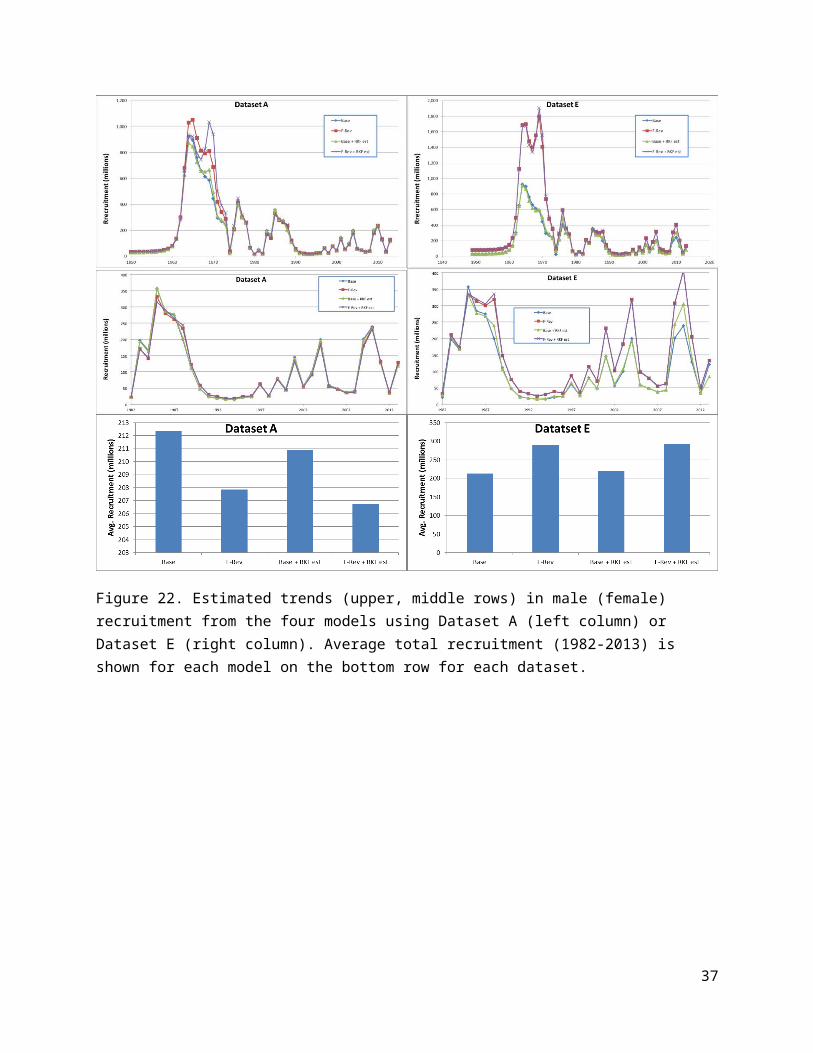
The estimated time series for recruitment from the “F-Rev” and “F-Rev+RKC est.” models for Dataset A are somewhat different in the mid-1960’s to early 1970’s time period, with peaks in estimated recruitment happening in different years, but otherwise they follow trajectories similar to one another, as well as to those of the base models (Fig. 22). Over the 1982-2013 time period, average recruitment is only slightly smaller for the F-Rev models than for the base models (~2%) for Dataset A. For Dataset E, the models estimating fishing mortality parameters associated with the BBRKC discard catch add only very small changes to the recruitment time series estimated by the base and F-Rev models, while the trajectories estimated by the base and F-Rev models are quite different in the mid-1960s-early-1970s but fairly similar from 1982 onward. However, the F-Rev models estimate higher peaks in recruitment during this latter period compared with the base model, which results in ~35% higher estimated average recruitment.

Recommendations

Data RevisionsIt would be worthwhile if the discrepancies (numbers of crab measured) between the size frequencies in the new datasets based on at-sea and dockside observer sampling in the various crab fisheries could be resolved with those used in previous assessments. If possible, computer codes (e.g., SQL scripts) used to generate the old and new datasets should be compared and differences identified. However, given changes in analysts over time, this may not be possible in most cases. In these cases, some double checking and vetting of the new data must occur in order to promote confidence in its reproducibility. The CPT should identify suitable procedures and a time frame for this vetting process. In particular, stock assessment analysts will need the vetted data much sooner than the fall assessment season in order to incorporate it into each assessment.

I would like to request that the CPT approve the changes I’ve made to handle size frequency data on Tanner crab bycatch from the groundfish fisheries (i.e., use the crab fishery year as a basis for compiling the size frequencies, use the datafiles extracted by R. Foy as the basis for these frequencies) and to replace the data previously used in the assessment to the new data based on these changes.

9

Model RevisionsI recommend adopting the revised model for fishing mortality used in the “F-Rev” models (and Gmacs) for the Tanner crab assessment model. Although the current formulation certainly works in that it fits both total catch and retained catch for males in the directed fishery, the interpretation of the functions comprising the directed fishing model is non-standard and can lead to communicating results effectively. In previous assessments, its “retention function” has been mis-interpreted even by the authors of the assessment as directly reflecting the on-deck sorting process. In addition, use of the new model appears to improve overall model fit to the data.

Literature CitedCrab Plan Team. 2014. Crab Modeling Report. https://npfmc.legistar.com/View.ashx?

M=F&ID=2865420&GUID=4C36935D-865B-4880-8A3A-D93CACC3C37CWhitten, A.R., A.E. Punt, J.N. Ianelli. 2013. Gmacs: Generalized Modeling for Alaskan Crab Stocks.

http://www.afsc.noaa.gov/REFM/stocks/Plan_Team/crab/Whitten%20et%20al%202014%20-%20Gmacs%20Model%20Description.pdf

Rugolo, L.J., and B.J. Turnock. 2012. 2012 Stock Assessment and Fishery Evaluation Report for the Tanner Crab Fisheries of the Bering Sea and Aleutian Islands Regions. In: Stock Assessment and Fishery Evaluation Report for the King and Tanner Crab Fisheries of the Bering Sea and Aleutian Islands: 2012 Crab SAFE. North Pacific Fishery Management Council. Anchorage, AK. pp. 267-416.

Stockhausen, W.T., B.J. Turnock and L. Rugolo. 2013. 2013 Stock Assessment and Fishery Evaluation Report for the Tanner Crab Fisheries of the Bering Sea and Aleutian Islands Regions. In: Stock Assessment and Fishery Evaluation Report for the King and Tanner Crab Fisheries of the Bering Sea and Aleutian Islands: 2013 Crab SAFE. North Pacific Fishery Management Council. Anchorage, AK. pp. 342-449.

10



https://npfmc.legistar.com/View.ashx?M=F&ID=2865420&GUID=4C36935D-865B-4880-8A3A-D93CACC3C37C

https://npfmc.legistar.com/View.ashx?M=F&ID=2865420&GUID=4C36935D-865B-4880-8A3A-D93CACC3C37C

Tables

Table 1. Potential revisions to the input data for the Tanner crab model considered in the analysis.

ID Description

A 2013 assessment data

BA + corrected sample sizes for bycatch size frequencies in the groundfish fisheries + corrected size frequencies for immature, new shell females in the 2013 AFSC trawl survey + very minor correction to csample sizes used for discard size frequencies in the crab fisheries

CB + recalculated retained size frequencies (1991-2009) based on new results from W. Gaeuman (ADFG)

DC + recalculated total catch size frequencies (1992-2012) in all crab fisheries based on new results from W. Gaeuman (ADFG)

ED + recalculated bycatch size frequencies (1973-2012) in the groundfish fisheries based on new results from R. Foy (NMFS)

Table 2. Number of measured male crab in dockside sampling for retained size frequencies in the recalculated and 2013 datasets. W. Gaeuman (ADFG) did not provide recalculated size frequencies for 1995.

year new shell old shell new shell old shell new shell old shell1991 117,630 8,669 117,630 8,669 0 01992 113,319 11,874 113,319 11,874 0 01993 67,264 4,358 67,264 4,358 0 01994 25,585 2,073 25,585 2,073 0 01995 0 0 495 1,030 -495 -1,0301996 2,063 2,367 2,063 2,367 0 02005 649 56 649 56 0 02006 1,053 1,887 1,053 1,887 0 02007 3,662 2,165 3,662 2,165 0 02008 2,717 344 3,146 344 -429 02009 2,369 48 13,903 412 -11,534 -364

2013 Assessment DifferenceRecalculated

11

Table 3. Number of Tanner crab measured by at-sea observers in the directed fishery in the recalculated and 2013 datasets.

Table 4. Number of Tanner crab measured by at-sea observers in the snow crab fishery for the recalculated and 2013 datasets.

12

Table 5. Number of Tanner crab measured by at-sea observers in the BBRKC fishery for the recalculated and 2013 datasets.

13

Table 6. Number of Tanner crab measured by at-sea observers in the groundfish fisheries for the recalculated and 2013 datasets. The recalculated dataset is based on the crab fishery year (starting July 1), whereas the 2013 assessment dataset was based on the groundfish fishery year (starting Jan. 1).

Females Males Females Males Females Males1973 2,279 3,155 1,212 1,604 1,067 1,5511974 1,624 2,500 2,789 4,155 -1,165 -1,6551975 839 1,254 24 16 815 1,2381976 6,709 6,984 2,526 2,928 4,183 4,0561977 8,401 10,703 9,803 10,873 -1,402 -1701978 13,801 18,699 8,105 11,724 5,696 6,9751979 11,360 19,075 16,953 24,924 -5,593 -5,8491980 5,984 12,890 5,598 10,424 386 2,4661981 4,127 6,122 6,817 12,956 -2,690 -6,8341982 8,161 13,681 5,694 7,690 2,467 5,9911983 8,335 18,404 7,983 14,112 352 4,2921984 14,288 27,849 10,589 24,303 3,699 3,5461985 12,823 23,290 12,765 26,334 58 -3,0441986 7,664 14,922 1,776 3,222 5,888 11,7001987 15,967 23,620 1,689 3,308 14,278 20,3121988 7,199 10,658 1,922 3,082 5,277 7,5761989 41,315 60,089 2,190 2,814 39,125 57,2751990 11,558 24,652 1,983 3,017 9,575 21,6351991 3,494 6,828 6,155 14,432 -2,661 -7,6041992 1,183 3,134 1,749 4,903 -566 -1,7691993 369 1,258 279 1,148 90 1101994 1,832 3,706 328 854 1,504 2,8521995 2,675 3,946 2,248 4,404 427 -4581996 3,410 8,370 2,364 3,458 1,046 4,9121997 3,912 9,972 5,314 12,176 -1,402 -2,2041998 4,448 12,150 4,282 10,139 166 2,0111999 4,528 11,066 4,399 12,037 129 -9712000 3,097 12,931 3,701 12,391 -604 5402001 3,100 15,821 2,485 12,910 615 2,9112002 3,252 15,418 3,232 15,498 20 -802003 2,763 9,613 3,292 13,542 -529 -3,9292004 4,479 13,876 2,788 11,110 1,691 2,7662005 3,711 17,796 4,097 13,424 -386 4,3722006 3,050 15,916 3,498 17,129 -448 -1,2132007 3,588 15,552 3,150 17,513 438 -1,9612008 3,869 23,997 2,832 10,658 1,037 13,3392009 2,493 17,642 1,973 6,435 520 11,2072010 1,571 6,323 2,096 5,952 -525 3712011 3,515 7,042 697 2,055 2,818 4,9872012 1,850 3,538 1,845 3,478 5 60

Crab Fishery Year

2013 AssessmentRecalculated Difference

14

Figures

Area of Enlargement

54°36' N Latitude

Western Subdistrict

168°

W L

ongi

tude

173°

W L

ongi

tude

BERING SEA DISTRICTCLOSED

Eastern Subdistrict

166°

W L

ongi

tudeGeneral Section

Norton SoundSection

61°49' N Latitude

Figure 1. Eastern Bering Sea District of Tanner crab Registration Area J including sub-districts and sections (from Bowers et al. 2008).

Figure 2. Size frequencies for immature, new shell females from the 2013 AFSC trawl survey: version used in the 2013 assessment (blue) and corrected version (red).

15

Figure 3. Corrected sample sizes for sex-specific (males: blue; females: red) bycatch size frequencies in the groundfish fisheries. The sexes were switched in the 2013 (and 2012) assessments.

Figure 4. Comparison of numbers of measured male crab, by year, in new/old shell categories in dockside sampling for retained Tanner crab in the recalculated dataset (red and blue lines) and the 2013 assessment dataset (green and purple lines).

Figure 5. Comparison of normalized dockside retained size frequencies from recalculated results (blue) and used in the 2013 assessment (red). Upper: 2008 new shell males. Middle: 2009 new shell males. Lower: 2009 old shell males.

16

Figure 6. Comparison of numbers of measured crab, by year and sex, in at-sea sampling in the directed Tanner crab fishery in the recalculated dataset (red and blue lines) and the 2013 assessment dataset (green and purple lines).

Figure 7. Comparison of numbers of measured Tanner crab, by year and sex, in at-sea sampling in the snow crab fishery in the recalculated dataset (red, blue lines) and the 2013 assessment (green, purple lines).

Figure 8. Comparison of numbers of measured Tanner crab, by year and sex, in at-sea sampling in the BBRKC fishery in the recalculated dataset (red, blue lines) and the 2013 assessment (green, purple lines).

17

Figure 9. Comparison of numbers of measured Tanner crab, by year and sex, in at-sea sampling in the groundfish fisheries in the recalculated dataset (red, blue lines) and the 2013 assessment (green, purple lines). The recalculated dataset is based on the crab fishery year (starting July 1), whereas the 2013 assessment dataset was based on the groundfish fishery year (starting Jan. 1).

Figure 10. Comparison of TCSAM2013-estimated MMB at mating time for the 5 datasets. Upper left: full time series. lower left: recent trends. Upper right: final (2012) estimates. Lower right: % change in final estimates relative to assessment dataset (A).

18

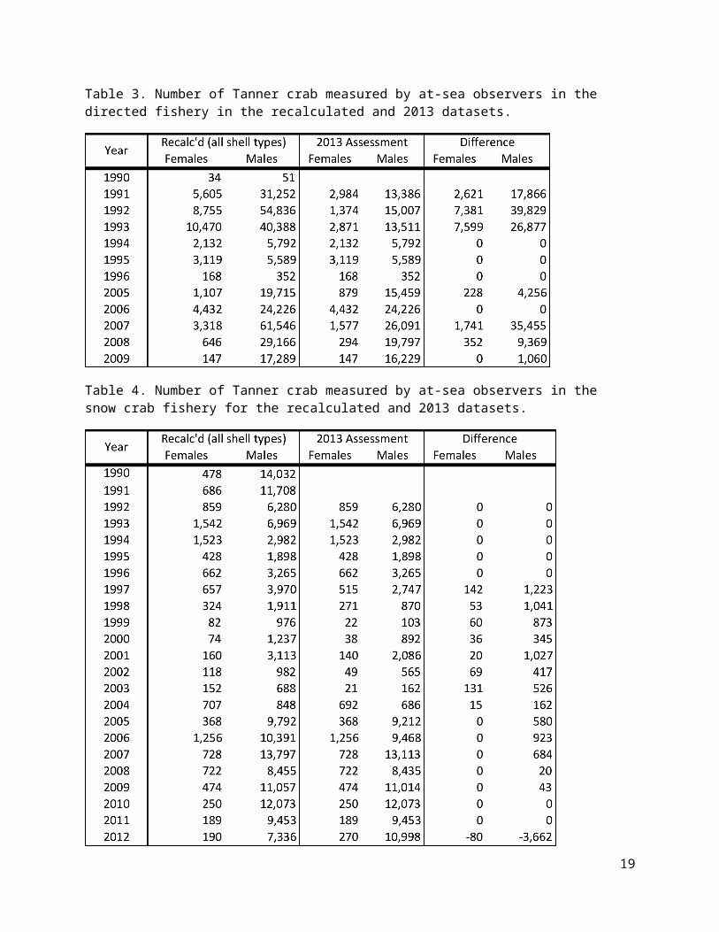
Figure 11. Comparison of TCSAM2013-estimated recruitment for the 5 datasets. Upper left: full time series for males. Lower left: recent trends in males. Upper right: 1982-2013 average. Lower right: % change in 1982-2013 average relative to assessment dataset (A).

Figure 12. Comparison of TCSAM2013-estimated directed fishing mortality for the 5 datasets. Left: full time series. Right: recent trends.

19

Figure 13. Objective function values obtained for the 5 datasets using TCSAM2013.

Figure 14. Comparison of objective function components obtained for the 5 datasets using TCSAM2013: differences between values obtained with the assessment dataset (A) and subsequent datasets. Positive values indicated better model fits obtained using a subsequent dataset.

Figure 15. Comparison of total objective function values for the 2013 assessment model (“Base”) and the 3 model revisions for the models run using Dataset A (left plot) and Dataset E (right plot).

20

Figure 16. Comparison of changes in objective function components obtained from the 3 model revisions using the 2013 assessment data (Dataset A) relative to the 2013 assessment model (Base). Positive values indicated better model fits obtained using the revised model.

Figure 17. Comparison of changes in objective function components obtained from the 3 model revisions using Dataset E relative to the 2013 assessment model (Base). Positive values indicated better model fits obtained using the revised model.

21

Figure 18. Estimated retention curves in two time periods for males in the directed fishery from the four models using Dataset A (left column) or Dataset E (right column).

22

dataset:model A E

Base

F-Rev

Base + RKF est

F-Rev + RKF est

Figure 19. Total selectivity on males in the directed fishery for each model (rows) using Dataset A (left column) or E (right column). Bold line in each plot is the selectivity curve used for years prior to 1991.

23

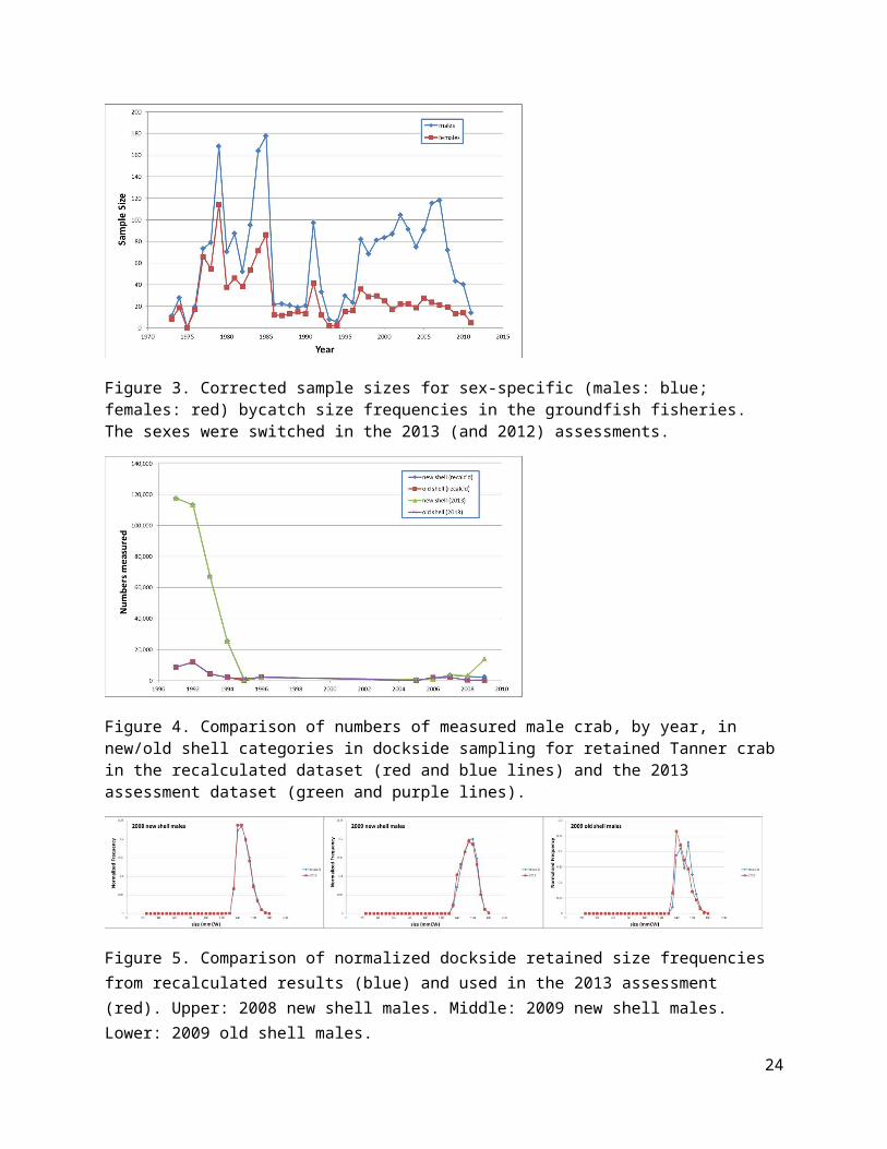
Figure 20. Estimated trends in fully-selected total fishing mortality/capture rate on males in the directed fishery from the four models using Dataset A (left column) or Dataset E (right column).

24

Figure 21. Estimated trends (upper, middle rows) in MMB from the four models using Dataset A (left column) and Dataset E (right column). MMB in the final model year (2012) is shown for each model on the bottom row for each dataset.

25

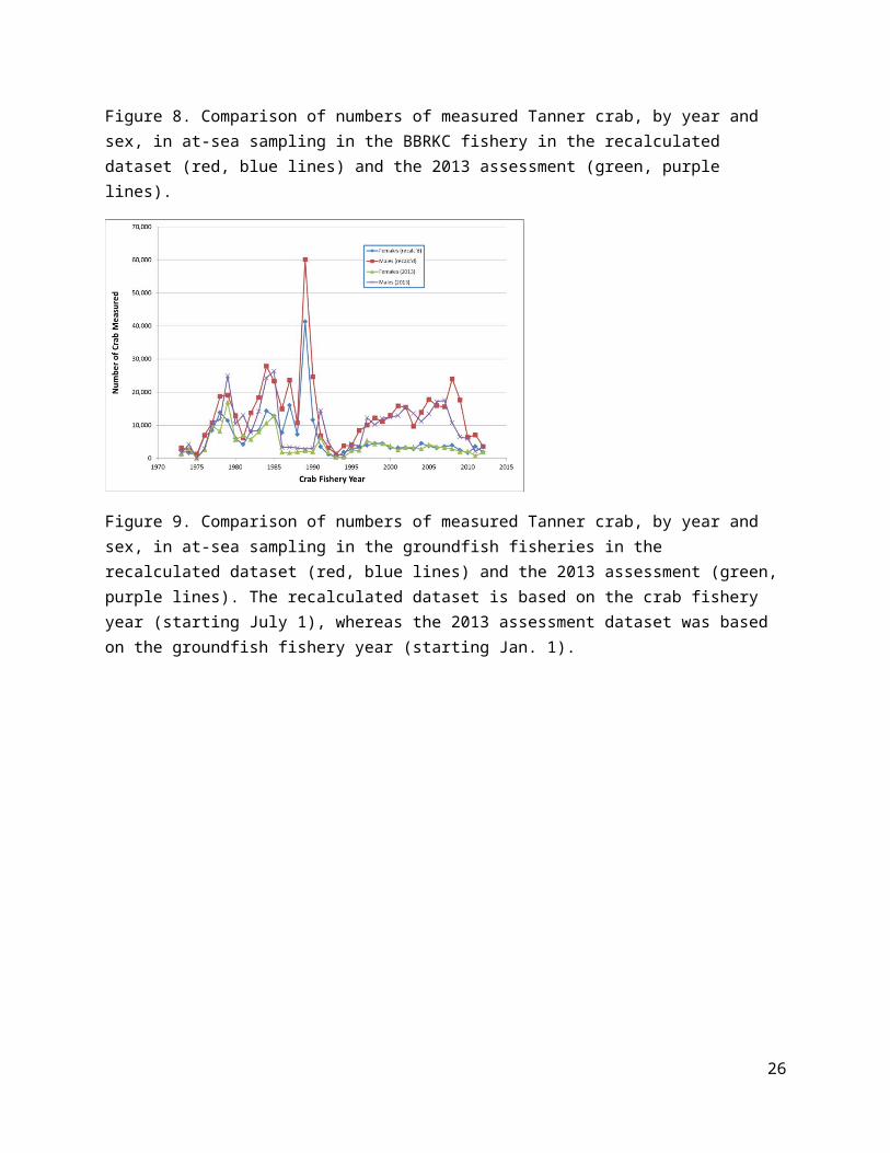
Figure 22. Estimated trends (upper, middle rows) in male (female) recruitment from the four models using Dataset A (left column) or Dataset E (right column). Average total recruitment (1982-2013) is shown for each model on the bottom row for each dataset.

26

Appendix 1: TCSAM (Tanner Crab Stock Assessment Model) 2013 Description

IntroductionThe Tanner crab stock assessment model (TCSAM) is an integrated assessment model developed with AD Model Builder (ref.) and C++ code that is fit to multiple data sources. The model described herein is the version used in the Sept. 2013 assessment (ref.) and will be referred to as TCSAM2013. Except for some corrections to the code, this model was identical to that used in the Sept. 2012 assessment (ref.).

Model parameters in TCSAM2013 are estimated using a maximum likelihood approach, with Bayesian-like priors on some parameters and penalties for smoothness and regularity on others. Data components entering the likelihood include fits to survey biomass, survey size compositions, retained catch, retained catch size compositions, discard mortality in the bycatch fisheries, and discard size compositions in the bycatch fisheries. Population abundance at the start of year y in the model, n y, x , m,s , z, is characterized by sex x (male, female), size z (carapace width, CW), maturity state m (immature, mature) and shell condition s (new shell, old shell). Changes in abundance due to natural mortality, molting and growth, maturation, fishing mortality and recruitment are tracked on an annual basis. Because the principal crab fisheries occur during the winter, the model year runs from July 1 to June 30 of the following calendar year.

A. Calculation sequence

Step A1: Survival prior to fisheriesNatural mortality is applied to the population from the start of the model year (July 1) until just prior to prosecution of the pulse fisheries for year y at δt y

F. The numbers surviving at δt yF in year y are given by:

n y, x , m,s , z1 =e−M y ,x,m ,s , z

❑ ∙ δt yF

∙ ny , x ,m ,s , z❑ A1

where M represents the annual rate of natural mortality in year y on crab classified as x, m, s, z.

Step A2: Prosecution of the fisheriesThe directed fishery and bycatch fisheries are modeled as pulse fisheries occurring at δt y

F in year y. The numbers that remain after the fisheries are prosecuted are given by:

n y, x , m,s , z2 =(1−e−F y ,x, m, s ,z

T ) ∙ ny , x ,m , s , z1 A2

where FT represents total (across all fisheries) annual fishing mortality in year y on crab classified as x, m, x, z.

Step A3: Survival after fisheries to time of molting/matingNatural mortality is again applied to the population from just after the fisheries to the time at which molting/mating occurs for year y at δt y

m. The numbers surviving at δt ym in year y are then given by:

n y, x , m ,s , z3 =e−M y , x,m ,s , z

❑ ∙(δt¿¿ ym−δt yF) ∙ ny ,x, m, s ,z

2 ¿ A3

where, as above, M represents the annual rate of natural mortality in year y on crab classified as x, m, s, z. In the 2012 and 2013 assessments, molting and mating were taken to occur on Feb. 15 each year (δt y

m=0.625), and the pulse fisheries were taken to occur just prior to this (δt yF=0.625, also), so the term

in the exponent in eq. A3 was 0 for all years.

27

Step A4: Molting, growth, and maturationThe changes in population structure due to molting, growth and maturation of immature (new shell) crab, as well as the change in shell condition for new shell mature crab due to aging, are given by:

n y, x , MAT , NS, z4 =∑

z'

❑

Θ y , x , z , z'MAT ∙ ϕ y , x, z'

❑ ∙n y , x, IMM , NS , z'3

A4a

n y, x , IMM , NS ,z4 =∑

z'

❑

Θ y , x , z , z'IMM ∙(1−ϕ y , x, z'

❑ )∙ ny , x , IMM , NS, z'3

A4b

n y, x , MAT ,OS , z4 =ny , x , MAT ,OS , z

3 +n y ,x , MAT , NS ,z3 A4c

where ϕ y , x , z❑ is the probability that an immature (new shell) crab of sex x and size z will undergo its

terminal molt to maturity and Θ y , x , z , z'm is the growth transition matrix from size z’ to z for that crab, which

may depend on whether (m=MAT; eq. A.4a) or not (m=IMM; eq. A.4b) the terminal molt to maturity occurs. Additionally, crabs that underwent their terminal molt to maturity the previous year are assumed to change shell condition from new shell (NS) to old shell (OS; A.4c). Note that the numbers of immature, old shell crab are identically zero in the current model because immature crab are assumed to molt each year until they undergo the terminal molt to maturity; consequently, an equation for m=IMM, s=NS above is unnecessary.

Step A5: Survival to end of year, recruitment, and update to start of next yearFinally, population abundance at the start of year y+1 due to recruitment of immature new shell crab at the end of year y (ry,x,z) and natural mortality on crab from the time of molting in year y until the end of the model year (June 30) are given by:

r y, x , z=R y ∙ ρy , x ∙ η z A5a

n y+1 , x, m, s , z❑ ={e−M y ,x, IMM, NS,z

❑ ∙(1−δt ¿¿ ym)∙ n y,x , IMM ,NS ,z4 +r y, x, z¿m=IMM , s=NS

e−M y, x,m ,s , z❑ ∙(1−δt¿¿ ym) ∙n y, x,m ,s ,z

4 ¿otherwise

A5b

B. Model processes: natural mortalityNatural mortality rates in TCSAM2013 vary across 3 year blocks (model start-1979, 1980-1984,1985-model end) within which they are sex- and maturity state-specific but do not depend on shell condition or size. They are parameterized in the following manner:

M y , x ,m, s , z={ M x, m , sbase ∙ δM x ,m 1980≤ y ≤1984

M x ,m ,sbase ∙ δM x, m∙ δM x ,m

T otherwisenatural mortality rates

B1

B2

where y is year, x is sex, m is maturity state and s is shell condition, the M x , m ,sbase are user constants (not

estimated), and the δM x ,m and δM x ,mT are parameters (although not all are estimated).

Priors are imposed on the δM x ,m parameters in the likelihood using:

28

Pr ( δM x, m )=∙ e−( δMx ,m−μx,m )

2 ∙σ x ,m2 Prior probability function for δM x ,m B3

The μ’s and σ❑2 , along with bounds, initial values and estimation phases used for the parameters, as well

as the values for the constants, used in the 2013 model are:

parameters/constants

μx, m σ x ,m2 lower

boundupper bound

initial value phase code name

M MALE , IMM , NSbase -- -- -- -- 0.23 NA M_in(MALE)

M FEMALE , IMM , NSbase -- -- -- -- 0.23 NA M_in(FEMALE)

M MALE , MAT , NSbase -- -- -- -- 0.23 NA M_matn_in(MALE)

M FEMALE , MAT , NSbase

-- -- -- --0.23 NA M_matn_in(FEMALE

)

M MALE , MAT ,OSbase -- -- -- -- 0.23 NA M_mato_in(MALE)

M FEMALE , MAT , OSbase

-- -- -- --0.23 NA M_mato_in(FEMALE

)

δM x , IMM1.0 0.05 0.2 2.0 1.1 7 M_mult_imat

δM MALE ,MAT1.0 0.05 0.1 1.9 1.0 7 Mmultm

δM FEMALE , MAT1.0 0.05 0.1 1.9 1.0 7 Mmultf

δM MALE ,IMMT -- -- -- -- 1.0 NA NA

δM FEMALE , IMMT -- -- -- -- 1.0 NA NA

δM MALE ,MATT 0.1 10.0 1.0 7 mat_big(MALE)

δM FEMALE , MATT 0.1 10.0 1.0 7 mat_big(FEMALE)

where constants have phase = NA and estimated parameters have phase > 0. When no corresponding variable exists in the model (code name = NA), the effective value of the parameter/constant is given.

29

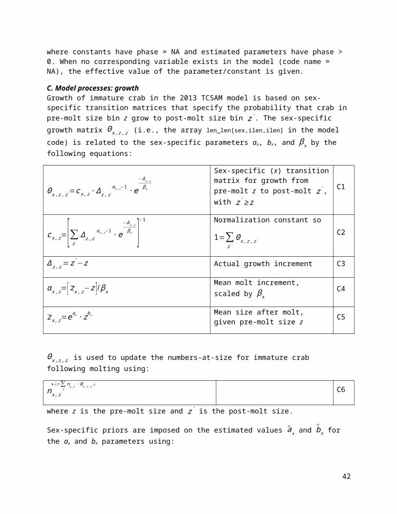
C. Model processes: growthGrowth of immature crab in the 2013 TCSAM model is based on sex-specific transition matrices that specify the probability that crab in pre-molt size bin z grow to post-molt size bin z '. The sex-specific growth matrix Θ x, z , z' (i.e., the array len_len[sex,ilen,ilen] in the model code) is related to the sex-specific parameters ax, bx, and βx by the following equations:

Θ x, z , z'=cx , z ∙ ∆ z , z'α x ,z−1 ∙ e

−∆z , z'

βx

Sex-specific (x) transition matrix for growth from pre-molt z to post-molt z ', with z ' ≥ z

C1

c x, z=[∑z '

∆z ,z 'α x ,z−1 ∙ e

−∆z , z'

βx ]−1 Normalization constant so

1=∑z'

Θ x , z , z'

C2

∆ z , z'=z '−z Actual growth increment C3

α x , z= [ zx , z−z ] / βx Mean molt increment, scaled by βx C4

zx , z=eax ∙ zbx Mean size after molt, given pre-molt size z C5

Θ x, z , z' is used to update the numbers-at-size for immature crab following molting using:

nx , z'

+¿=∑z

nx, z' ∙Θ x, z ,z' ¿C6

where z is the pre-molt size and z ' is the post-molt size.

Sex-specific priors are imposed on the estimated values ax and bx for the ax and bx parameters using:

Pr ( ax)=∙ e

−( ax−μax)2 ∙σ ax

2 Prior probability function for a’s C7

Pr ( bx)=∙ e−( bx−μbx )

2 ∙ σbx

2 Prior probability function for b’s C8

The μ’s and σ❑2 , along with the bounds, initial values and estimation phases used for the parameters in the

2013 TCSAM are:

parameter sex (x) μx σ x2 lower

boundupper bound


ax female 0.56560241 0.100 0.4 0.7 0.55 8af1

30

male 0.43794100 0.025 0.3 0.6 0.45 8 am1

bx

female 0.9132661 0.025 0.6 1.2 0.90 8 bf1

male 0.9487000 0.100 0.7 1.2 0.95 8 bm1

βx both NA NA 0.75000 0.75001 0.750005 -2 growth_beta

Note that the βx are treated as constants because the associated estimation phases are negative.

D. Model processes: maturityMaturation of immature crab in TCSAM2013 model is based on sex- and size-specific probabilities of maturation, ϕ x ,z, where size z is pre-molt size. After molting, but before assessing growth, the numbers of crab remaining immature, nx , IMM , NS

+¿ ( z) ¿ , and those maturing, nx , MAT ,NS+¿ ( z) ¿ , at pre-molt size z are given by:

¿D1a

D1b

where nx , IMM , NS(z ) is the number of immature, new shell crab of sex x at pre-molt size z.

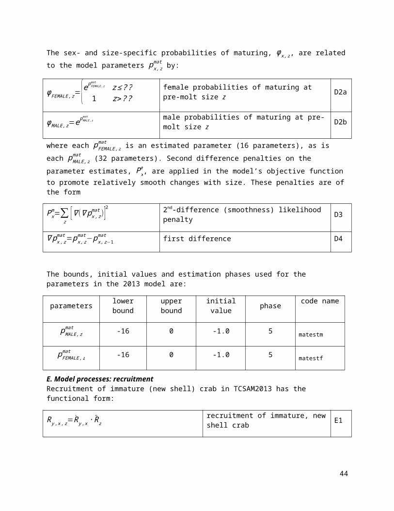
The sex- and size-specific probabilities of maturing, ϕ x ,z, are related to the model parameters px, zmat by:

ϕ FEMALE , z={e pFEMALE ,zmat

z≤ ? ?1 z>? ?

female probabilities of maturing at pre-molt size z D2a

ϕ MALE, z=ep MALE, zmat

male probabilities of maturing at pre-molt size z D2b

where each pFEMALE , zmat is an estimated parameter (16 parameters), as is each pMALE, z

mat (32 parameters). Second difference penalties on the parameter estimates, P x

m, are applied in the model’s objective function to promote relatively smooth changes with size. These penalties are of the form

P xm=∑

z[∇ (∇ px , z

mat)]2 2nd-difference (smoothness) likelihood penalty D3

∇ px , zmat=px, z

mat−px , z−1mat first difference D4

The bounds, initial values and estimation phases used for the parameters in the 2013 model are:

parameters lower bound upper bound initial value phase code name

31

pMALE, zmat -16 0 -1.0 5 matestm

pFEMALE , zmat -16 0 -1.0 5 matestf

E. Model processes: recruitmentRecruitment of immature (new shell) crab in TCSAM2013 has the functional form:

R y , x , z=R y , x ∙ R z recruitment of immature, new shell crab E1

where y is year, x is sex, and z is size. R y , x represents total sex-specific recruitment in year y and R z represents the size distribution of recruits, which is assumed identical for males and females.

Sex-specific recruitment, R y , x, is parameterized as

R y , x={e pLnRH+ δRyH

y≤ 1973e pLnR+δRy 1974 ≤ y

sex-specific recruitment of

immature, new shell crabE2

where the sex ratio at recruitment is assumed to be 1:1 and the δR yand δR yH are “devs” parameter vectors,

with the constraint that the elements of a “devs” vector sums to zero. Independent parameter sets are used for the “historic” period during model spin-up (1949-1973) and the “current” period (1974-2013).

The size distribution for recruits, R z, is based on a gamma-type distribution and is parameterized as

R z=c−1∙∆ z

αβ

−1∙ e

−∆z

β size distribution of recruiting crab E3

where α and β are parameters, ∆ z=z+2.5−zmin, and c=∑z

∆ z

αβ

−1∙ e

−∆z

β is a normalization constant so

that 1=∑z

R z. zmin is the smallest model size bin (27 mm) and the constant 2.5 represents one-half the

size bin spacing.

Penalties are imposed on the “devs” parameter vectors δR yand δR yH in the objective function as follows:

P (δR )=∑y

δR y2

Penalty function on δR y E4

P (δRH )=∑y

(δR yH−δRy−1

H )2 1st difference penalty function on δR yH E5

The bounds, initial values and estimation phases used for the parameters used in the 2013 model are:

parameters lower bound

upper bound


32

pLnRH -- -- 0.0 1 pMnLnRecEarly

pLnR -- -- 11.4 1 pMnLnRec

δR yH -15 15 0 1 pRecDevsEarly

δR y-15 15 0 1 pRecDevs

α 11.49 11.51 11.50 -8 alpha1_rec

β 3.99 4.01 4.00 -8 beta_rec

where parameters with phase < 0 are not estimated (i.e., treated as constants).

F. Model processes: fisheriesFour fisheries that catch Tanner crab are included in TCSAM2013: 1) the directed Tanner crab fishery, 2) the snow crab fishery, 3) the BBRKC fishery and 4) the various groundfish fisheries (lumped as one bycatch fishery). Crab (males only) are assumed to be retained exclusively in the directed fishery. Bycatch of non-retained Tanner crab (males and females) is assumed to occur in all four fisheries; discard mortality fractions for the (discarded) bycatch are assumed to differ between the crab and groundfish fisheries due to the differences in gear used (pots vs. primarily bottom trawl).

The predicted number of crab killed in fishery f by year in TCSAM2013 model has the functional form:

m y , x ,m, s , zf =

F y ,x , m,s , zf

F y ,x , m,s , zT ∙ [1−e−F y ,x ,m ,s ,z

T ] ∙ ny , x ,m ,s , z1 estimated crab mortality in fishery f F1

where y is year, x is sex, m is maturity state, s is shell condition and z is size, F y , x, m, s ,zf is sex/maturity

state/shell condition/size-specific fishing mortality in year y, and F y , x, m, s ,zT =∑

fF y , x, m , s , z

f is total fishing

mortality sex x crab in maturity state m and shell condition s at size z at the time the fisheries occur in year y. Note that m y , x ,m, s , z

f represents the estimated mortality in numbers associated with fishery f, not the numbers captured (i.e., brought on deck). These differ because discard mortality is not 100% in the fisheries).

The total fishing mortality rate for each fishery is decomposed into two multiplicative components: 1) the mortality rate on fully-selected crab, FM y

f , and 2) a size-specific selectivity function Sy , x ,m, s , zf , as

follows:

F y , x, m, s ,zf =FM y

f ∙ S y , x ,m, sf fishing mortality rate in fishery f F2

33

Fully-selected fishing mortalityThe manner in which the fully-selected fishing mortality rate is further decomposed is time-dependent and specific to each fishery. Consequently, this decomposition is discussed below specific to each fishery.

Considering Tanner crab total fishing mortality (retained + discards) in the directed Tanner crab fishery (TCF) first, the fully-selected fishing mortality is modeled differently in three time periods:

FM yTCF={ 0.05 y<1965

0 1965 ≤ y , fishery closede p LnF TCF+δF y

TCF

1965 ≤ y , fishery open

fully-selected fishing mortality rate in the directed Tanner crab fishery

F3

where p LnFTCFis a parameter representing the mean ln-scale fishing mortality in the Tanner crab fishery since 1964 (catch data for this fishery begins in 1965) and δF y

TCF represents a “devs” parameter vector with elements defined for each year the fishery was open. Prior to 1965, a small directed fishing mortality rate (0.05) is assumed.

For Tanner crab bycatch in the snow crab fishery (SCF), the fully-selected discard fishing mortality is modeled differently in three time periods using:

FM ySCF={ 0.01 y<1978

r SCF ∙ E ySCF 1978≤ y ≤1991

ep LnF SCF+δFySCF

1992≤ y

fully-selected discard fishing mortality rate in the snow crab fishery

F4

where p LnFSCFis a parameter representing the mean ln-scale bycatch fishing mortality in the snow crab fishery since 1992 (when reliable observer-based Tanner crab discard data in the snow crab fishery first became available) and δF y

SCF represents a “devs” parameter vector with elements defined for each year in this time period. Prior to 1978, a small annual discard mortality rate associated with this fishery (0.01) is assumed. Annual effort data (total potlifts, E y

SCF) is used to extend predictions of Tanner crab discard mortality in this fishery into the period 1978-1991. To do this, the assumption is made that effort in the snow crab fishery is proportional to Tanner crab discard fishing mortality and estimate the proportionality constant, r SCF, using a ratio estimator between effort and discard mortality in the period 1992-present:

r SCF={ 1

N ∑y=1992

present

FM ySCF}

{ 1N ∑

y=1992

present

E ySCF}

ratio estimator relating fishing mortality rate to effort in the snow crab fishery

F5

where N is the number of years, 1992-present.

For Tanner crab bycatch in the BBRKC fishery (RKF), the fully-selected discard fishing mortality when the fishery was open is modeled differently in three time periods using:

34

FM yRKF={ 0.02 y<1953

max {0.01,−ln [1−r RKF ∙ E yRKF ] } 1953 ≤ y≤ 1991

e p LnF RKF+δF yRKF

1992≤ y

fully-selected discard fishing mortality rate in the BBRKC fishery

F6

where p LnFRKFis a parameter representing the mean ln-scale bycatch fishing mortality in the BBRKC fishery since 1992 (when observer-based Tanner crab discard data in the BBRKC fishery first became available) and δF y

RKF represents a “devs” parameter vector with elements defined for each year in this period that the fishery was open. Prior to 1953, a small annual discard mortality rate associated with this fishery (0.02) was assumed. Annual effort data (total potlifts, E y

RKF) was used to extend predictions of Tanner crab discard mortality in this fishery into the period 1953-1991. To do this, we made the assumption that effort in the BBRKC fishery is proportional to Tanner crab discard fishing mortality and estimate the proportionality constant, r RKF, using a ratio estimator between effort and discard mortality in the period 1992-present:

r RKF={ 1

N ∑y=1992

present

[1−e−FM yRKF ]}

{ 1N ∑

y=1992

present

E yRKF}

ratio estimator relating fishing mortality rate to effort in the BBRKC fishery

F7

where N is the number of years, 1992-present, when the BBRKC fishery was open. For any year that the BBRKC fishery was closed, FM y

RKF was set to 0.

Finally, for Tanner crab bycatch in the groundfish fisheries (GTF), the fully-selected discard fishing mortality in the fishery was modeled differently in two time periods using:

FM yGTF={ 1

N ∑y=1992

present

ep LnFGTF +δF yGTF

y<1973

ep LnFGTF+δF yGTF

1973≤ y

fully-selected discard fishing mortality rate in the groundfish trawl fisheries

F8

where p LnFGTFis a parameter representing the mean fully-selected ln-scale bycatch fishing mortality in the groundfish fisheries since 1973 (when observer-based Tanner crab discard data in the groundfish fisheries first became available) and δF y

GTF is a “devs” parameter vector with elements representing the annual ln-scale deviation from the mean. Prior to 1973, the fully-selected discard mortality rate associated with these fisheries was assumed to be constant and equal to the mean over the 1973-present period.

The bounds (when set), initial values and estimation phases used for the fully-selected fishing mortality parameters and devs vectors in the 2013 model were:


upper bound


p LnFTCF -- -- -0.7 1 pAvgLnFmTCF

35

δF yTCF -15 15 0 2 pFmDevsTCF

p LnF SCF -- -- -3.0 3 pAvgLnFmSCF

δF ySCF -15 15 0 4 pFmDevsSCF

p LnFRKF -5.25 -5.25 -5.25 -4 pAvgLnFmRKF

δF yRKF -15 15 0 -5 pFmDevsRKF

p LnFGTF -- -- -4.0 2 pAvgLnFmGTF

δF yGTF -15 15 0 3 pFmDevsGTF

where all parameters and parameter vectors were estimated (phase > 0), except for those associated with the BBRKC fishery.

Fishery selectivityThe manner in which fishery selectivity is parameterized is also time-dependent and specific to each fishery, as with the fully-selected fishing mortality. However, the time periods used to define selectivity are not necessarily those used for the fully-selected fishing mortality.

In the directed Tanner crab fishery (TCF), total selectivity (retained + discards) is modeled using sex-specific ascending logistic functions. For males, in addition, total selectivity is parameterized differently in three time periods, corresponding to differences in information about the fishery (pre-/post-1991) and differences in the fishery itself (pre-/post-rationalization in 2005):

Sy , FEMALE , m,s , zTCF ={1+e− pβ FEMALE

TCF ∙ (z−pZ50FEMALETCF )}−1

total selectivity for females in the directed Tanner crab fishery

F9

Sy , MALE ,m, s , zTCF ={ {1+e− pβMALE

TCF(1) ∙(z− z50MALETCF )}−1

y ≤1990

{1+e−pβ MALETCF (1) ∙(z− z50y ,MALE

TCF )}−11991≤ y ≤1996

{1+e−pβ MALETCF (2) ∙(z− z50y ,MALE

TCF )}−12005 ≤ y ≤ 2009

total selectivity for males in the directed Tanner crab fishery

F10

where the pβxTCF (t )are parameters controlling the slopes of the associated logistic selectivity curves,

pZ50FEMALETCF is the parameter controlling the size of females at 50% selection, z50MALE

TCF controls the size of 50%-selected males in the pre-1991 period, and z50 y , MALE

TCF controls the size of 50%-selected males in the post-1990 period. The latter three quantities are functions of estimable parameters as described in the following:

36

z50MALETCF =1

6 ∑y=1991

1996

z50 y , MALETCF male size at 50%-selected used in

pre-1991 period F11

z50 y , MALETCF =epLnZ50MALE

TCF +δZ 50y ,MALETCF male size at 50%-selected used in

post-1990 period F12

where pLn Z50MALETCF is a parameter controlling the ln-scale mean male size at 50% selectivity post-1990

and δZ 50 y, MALETCF is a parameter vector controlling annual ln-scale deviations in male size at 50% selectivity

post-1990. As formulated, selectivity in the directed fishery is not a function of maturity state or shell condition.

The bounds, initial values and estimation phases used in the 2013 model for the 5 parameters describing total selectivity in the directed Tanner crab fishery were:


upper bound


pβFEMALETCF 0.1 0.4 0.25 3 fish_disc_slope_f

pZ50FEMALETCF 80 150 115 3 fish_disc_sel50_f

pβMALETCF (1) 0.05 0.75 0.4 3 fish_slope_1

pβMALETCF (2) 0.1 0.4 0.25 3 fish_slope_yr_3

pLn Z50M ALETCF 4.0 5.0 4.5 3 log_avg_sel50_3

where all parameters were estimated. The bounds, initial values and estimation phase used in the 2013 model for the ln-scale “devs” parameter vector δZ 50 y, MALE

TCF describing annual deviations in male size at 50%-selected (1991-1996, 2005-2009) were:


upper bound


δZ 50 y, MALETCF -0.5 0.5 0 3 log_sel50_dev_3

In the snow crab fishery (SCF), bycatch (discard) selectivity is modeled using three time periods (model start to 1996, 1997-2004, 2005 to present). Male selectivity is described using dome-shaped (double logistic) functions in each period, with:

37

Sy , MALE ,m, s , zSCF ={SMALE , z

SCF(1) y ≤1996S MALE ,z

SCF (2) 1997 ≤ y ≤ 2004SMALE , z

SCF(3) 2005 ≤ y

male selectivity in the

snow crab fisheryF13

where the double logistic functions SMALE, zSCF (t ) are parameterized using:

SMALE, zSCF (t ) = {1+e−pβMALE

SCF (ta ) ∙ (z−pZ50MALESCF (ta ))}−1

∙ {1+e+ pβ MALESCF ( td) ∙ (z−pZ 50MALE

SCF( td ))}−1 dome-shaped selectivity

F14

where pβxSCF(ta)and pZ50x

SCF(ta) are the 6 parameters controlling the ascending limb of the double logistic function and pβx

SCF (td)and pZ50xSCF (td ) are the 6 parameters controlling the descending limb for each period

t.

Female selectivity is described using ascending logistic functions in each period, with:

Sy , FEMALE , m,s , zSCF ={SFEMALE , z

SCF (1) y ≤1996SFEMALE , z

SCF (2) 1997 ≤ y ≤2004SFEMALE , z

SCF (3) 2005 ≤ y

female selectivity in the snow crab fishery F15

where the ascending logistic functions SFEMALE , zSCF (t ) are parameterized using:

SFEMALE , zSCF (t ) ={1+e− pβFEMALE

SCF (t) ∙( z− pZ50 FEMALESCF (t ) )}−1

ascending logistic selectivity F16

where the pβxSCF( p)are the 3 parameters controlling the slopes of the associated logistic selectivity curves

and the pZ50xSCF (p ) are the 3 parameters controlling size at 50%-selection.

As formulated, selectivity in the snow crab fishery is not a function of maturity state or shell condition.

38

The bounds, initial values and estimation phases used in the 2013 model for the 12 parameters describing male selectivity in the snow crab fishery were:


upper bound


pβMALESCF (1a) 0.01 0.50 0.255 4 snowfish_disc_slope_m_1

pZ50MALESCF(1a ) 60 150 122.5 4 snowfish_disc_sel50_m_1

pβMALESCF (1d)

0.01 0.500.255 4 snowfish_disc_slope_m2_

1

pZ50MALESCF(1 d )

40 200120 4 snowfish_disc_sel50_m2_

1

pβMALESCF (2 a) 0.01 0.50 0.255 4 snowfish_disc_slope_m_2


pβMALESCF (2d)


2

pZ50MALESCF(2d )


2

pβMALESCF (3a) 0.01 0.50 0.255 4 snowfish_disc_slope_m_3


pβMALESCF (3 d)


3

pZ50MALESCF(3d )


3

where all parameters were estimated.

39

The bounds, initial values and estimation phases used in the 2013 model for the 6 parameters describing female selectivity in the snow crab fishery were:


upper bound


pβFEMALESCF (1)

0.05 0.50.275 4 snowfish_disc_slope_f

1

pZ50FEMALESCF(1 )

50 150100 4 snowfish_disc_sel50_f

1

pβFEMALESCF (2)


2

pZ50FEMALESCF(2 )


2

pβFEMALESCF (3)


3

pZ50FEMALESCF(3 )


3


In the BBRKC fishery (RKF), bycatch (discard) selectivity is also modeled using the three time periods used to model selectivity in the snow crab fishery (model start to 1996, 1997-2004, 2005 to present), with sex-specific parameters estimated in each period. All sex/period combinations are modeled using ascending logistic functions:

Sy , x ,m , s , zRKF ={{1+e− pβx

RKF (1) ∙(z− pZ50xRKF (1))}−1

y≤ 1996

{1+e− pβxRKF (2) ∙(z− pZ50x

RKF (2))}−11997 ≤ y≤ 2004

{1+e− pβxRKF (3) ∙(z− pZ50x

RKF (3))}−12005≤ y

selectivity in the BBRKC fishery F17

where the pβxRKF( p)are 6 parameters controlling the slopes of the associated logistic selectivity curves and

the pZ50xRKF ( p) are 6 parameters controlling size at 50%-selection. As formulated, selectivity in the

BBRKC fishery is not a function of maturity state or shell condition.

40

The bounds, initial values and estimation phases used in the 2013 model for the 12 parameters describing male selectivity in the BBRKC fishery were:


upper bound


pβMALERKF(1)

0.01 0.500.255 3 rkfish_disc_slope_m

1

pZ50MALERKF(1)

95 150122.5 3 rkfish_disc_sel50_m

1

pβMALERKF(2)


2

pZ50MALERKF(2)


2

pβMALERKF(3)


3

pZ50MALERKF(3)


3


41

The bounds, initial values and estimation phases used in the 2013 model for the 6 parameters describing female selectivity in the BBRKC fishery were:


upper bound


pβFEMALERKF(1)

0.005 0.500.2525 3 rkfish_disc_slope_f

1

pZ50FEMALERKF(1)

50 150100 3 rkfish_disc_sel50_f

1

pβFEMALERKF(2)


2

pZ50FEMALERKF(2)


2

pβFEMALERKF(3)


3

pZ50FEMALERKF(3)


3


In the groundfish fisheries (GTF), bycatch (discard) selectivity is also modeled using three time periods (model start to 1986, 1987-1996, 1997 to present), but these are different from those used in the snow crab and BBRKC fisheries. Sex-specific parameters are estimated in each period; all sex/period combinations are modeled using ascending logistic functions:

Sy , x ,m , s , zGTF ={{1+e− pβx

GTF( 1)∙ (z− pZ50xGTF (1) )}−1

y≤ 1986

{1+e− pβxGTF( 2)∙ (z− pZ50x

GTF (2) )}−11987 ≤ y ≤1996

{1+e− pβxGTF(3 )∙ (z− pZ50x

GTF (3) )}−11997 ≤ y

selectivity in the groundfish fisheries F18

where the pβxGTF (p )are 6 parameters controlling the slopes of the associated logistic selectivity curves and

the pZ50xGTF (p ) are 6 parameters controlling size at 50%-selection. As formulated, selectivity in the

groundfish fisheries is not a function of maturity state or shell condition.

42

The bounds, initial values and estimation phases used in the 2013 model for the 12 parameters describing male selectivity in the groundfish fisheries were:


upper bound


pβMALEGTF (1 )

0.01 0.500.255 3 fish_disc_slope_tm

1

pZ50MALEGTF (1)

40 120.0180.005 3 fish_disc_sel50_tm

1

pβMALEGTF (2 )


2

pZ50MALEGTF (2)

40 120.0180.005 3 fish_disc_sel50_tm

2

pβMALEGTF (3 )


3

pZ50MALEGTF (3)

40 120.0180.005 3 fish_disc_sel50_tm

3


43

The bounds, initial values and estimation phases used in the 2013 model for the 6 parameters describing female selectivity in the groundfish fisheries were:


upper bound


pβFEMALEGTF (1 )

0.01 0.500.255 3 fish_disc_slope_tf

1

pZ50FEMALEGTF (1)

40 125.0182.505 3 fish_disc_sel50_tf

1

pβFEMALEGTF (2 )


2

pZ50FEMALEGTF (2)

40 250.01145.005 3 fish_disc_sel50_tf

2

pβFEMALEGTF (3 )


3

pZ50FEMALEGTF (3)

40 150.0195.005 3 fish_disc_sel50_tf

3


Retention in the directed fisheryRetention of male crab in the directed fishery is modeled as a multiplicative size-specific process “on top” of total (retention + discards) fishing selectivity. The number of crab (males only) retained in the directed Tanner crab fishery is given by

r y, m, s ,zTCF =

R y , m,s , zTCF

F y , MALE ,m, s , zT ∙ [1−e−F y, MALE,m ,s , z

T ] ∙ ny , MALE, m,s , z1 retained male crab (numbers)

in the directed fishery F19

where R y , m ,s ,zTCF is the retained mortality rate associated with retention, which is related to the total fishing

mortality rate on male crab in the directed fishery, F y , MALE,m ,s , zTCF , by

R y , m,s ,zTCF =ρ y , m,s , z

TCF ∙F y , MALE ,m, s , zTCF =FM y

TCF ∙ ρy , m,s , zTCF ∙ S y , MALE, m,s

TCF retained mortality rate in the directed fishery F20

where ρ y , m , s ,zTCF represents size-specific retention of male crab. Retention at size, ρ y , m , s ,z

TCF , in the directed fishery is modeled as an ascending logistic function, with different parameters in two time periods, as follows:

44

ρ y , m, s ,zTCF ={{1+e−pβTCFR (1) ∙ (z−pZ 50

TCFR( 1))}−1y≤ 1990

{1+e−pβTCFR (2) ∙ (z−pZ 50TCFR( 2))}−1

1991≤ y

size-specific retention in the directed fishery F21

where pβTCFR (t ) is the parameter controlling the slope of the function in the each period (t=1,2) and pZ50

TCFR (t ) is the parameter controlling the size at 50%-selected. As formulated, retention is not a function of maturity state or shell condition.

The bounds, initial values and estimation phases used for the size-specific retention parameters in the 2013 model were:


upper bound


pβTCFR (1 ) 0.25 1.01 0.63 3 fish_fit_slope_mn1

pZ50TCFR (1) 85 160 122.5 3 fish_fit_sel50_mn1

pβTCFR (2 ) 0.25 2.01 1.13 3 fish_fit_slope_mn2

pZ50TCFR (2) 85 160 122.5 3 fish_fit_sel50_mn2


G. Model indices: surveysThe predicted number of crab caught in the survey by year in the 2013 TCSAM model has the functional form:

n y, x , m ,s , zsrv =q y ,x ∙ S y ,x , z ∙ ny , x, m, s , z predicted number of crab caught in survey G1

where y is year, x is sex, m is maturity state, s is shell condition and z is size, q y , xis sex-specific survey catchability in year y, Sy , x , z is sex-specific size selectivity in year y, and n y, x , m ,s , z is the number of sex x crab in maturity state m and shell condition s at size z at the time of the survey in year y.

Three time periods that were used to test hypotheses regarding changes in catchability and selectivity in the survey over time are defined in the model. These periods are defined as: 1) y<1982, 2) 1982 ≤ y ≤1987, and 3) 1988 ≤ y . As parameterized in the 2013 model, catchabilities in periods 2 and 3 were assumed to be identical, so only two sets of sex-specific parameters reflecting catchability were used in the model. In terms of the three time periods, catchability was parameterized using the sex-specific parameters qx

I and qxII in the following manner:

q y , x={qxI y<1982

qxII 1982 ≤ y ≤ 1987

qxII 1988 ≤ y

survey catchability G2

45

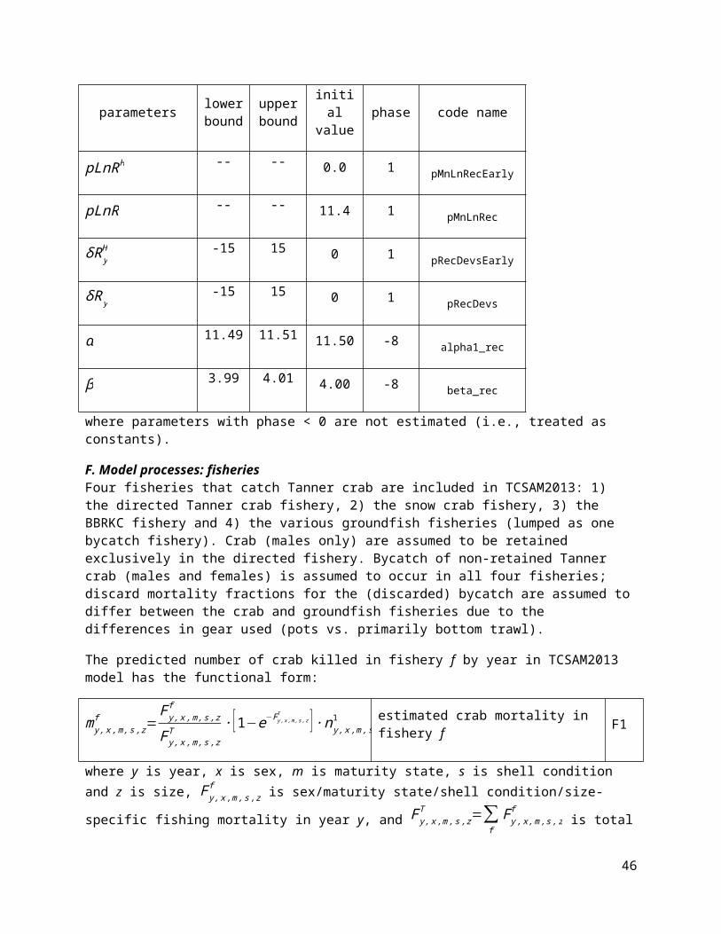
The bounds, initial values and estimation phases used for these parameters in the 2013 model were:


upper bound


qMALEI 0.50 1.001 0.7505 4 srv2_q

qFEMALEI 0.50 1.001 0.7505 4 srv2_femQ

qMALEII 0.20 2.00 1.1 4 srv3_q

qFEMALEII 0.20 1.00 0.6 4 srv3_femQ

where all parameters were estimated (phase > 0).

Similarly, survey selectivity in periods 2 and 3 was assumed identical and only two sets of sex-specific parameters were used to describe survey selectivity using logistic functions:

Sy , z={{1+e−[ ln (19) ∙(z− z50xI )/δ z95x

I ] }−1y<1982

{1+e−[ ln (19) ∙( z−z50 xII )/δz 95x

II ] }−11982≤ y ≤1987

{1+e−[ ln (19)∙( z−z50xII )/δ z95x

II ] }−11987 ≤ y

survey selectivity G3

where the z50’s are parameters reflecting the inflection point of the logistic curve (i.e., size at 50% selected) and the δz 95’s are parameters reflecting the difference the sizes at 50% and 95% selected.

46

The bounds, initial values and estimation phases used for the selectivity parameters used in the 2013 model were:


upper bound


z50MALEI 0 90 45 4 srv2_sel50

z50FEMALEI -200 100.01 -49.005 4 srv2_sel50_f

δz 95MALEI 0 100 50 4 srv2_seldiff

δz 95FEMALEI 0 100 50 4 srv2_seldiff_f

z50MALEII 0 69 34.5 4 srv3_sel50

z50FEMALEII -50 69 9.5 4 srv3_sel50_f

δz 95MALEII 0 100 50 4 srv3_seldiff

δz 95FEMALEII 0 100 50 4 srv3_seldiff_f

where all parameters were estimated (phase > 0).

H. Model fitting: objective function equationsThe TCSAM2013 model is fit by minimizing an objective function, o, with additive components consisting of: 1) several penalty functions, 2) several negative log-likelihood functions based on assumed prior probability distributions for model parameters, and 3) several negative log-likelihood functions based on input data components, of the form:

o=∑f

λ f ∙F f −2∑p

λp ∙ ln (℘p )−2∑l

λl ∙ ln (Ll) model objective function H1

where F f represents the fth penalty function, ℘p represents the pth prior probability function, Ll represents the lth likelihood function, and the λ’s represent user-adjustable weights for each component.

Penalty FunctionsThe penalty functions associated with various model quantities are identified in the section (B-F) concerning the associated process.

Prior Probability FunctionsThe prior probability functions associated with various model parameters are identified in the section (B-F) concerning the associated parameter.

47

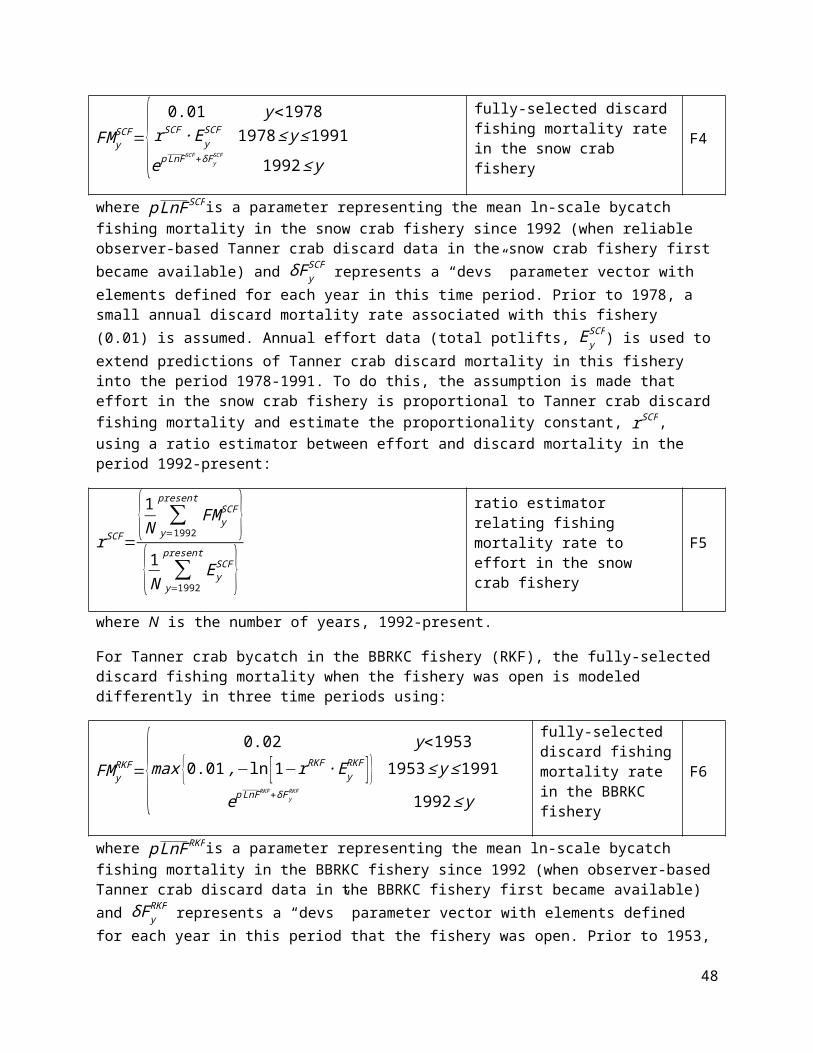
Likelihood FunctionsThe model’s objective function includes likelihood components based on 1) retained catch size frequencies (i.e., males only) in the directed fishery from dockside observer sampling; 2) total catch (retained + discarded) size frequencies by sex in each fishery from at-sea observer sampling; 3) size frequencies for immature males, mature males, immature females, and mature females, respectively, from trawl survey data; 4) dockside retained catch biomass (i.e., males only) in the directed fishery from fish ticket data; 5) estimated total catch (retained + discarded) mortality in biomass by sex in the crab and groundfish fisheries from at-sea observer sampling; and 6) estimated mature biomass by sex from trawl survey data. As discussed in more detail below, size frequency-related likelihood components are based on the multinomial distribution while those related to biomass are based on either the normal or lognormal distributions.

Size frequency componentsFishery-related (log-scale) likelihood components involving sex-specific size frequencies are based on the following equation for multinomial sampling:

ln ( LM )xf=∑

yny , x

f ∙∑z

py , x , zobs .f ∙ ln ( p y ,x , z

mod .f +δ )−py , x , zobs . f ∙ ln ( p y , x, z

obs. f +δ ) multinomial log-likelihood H2

where f indicates the fishery, x indicates sex, the y’s are years for which data exists, n y, xf is the sex-

specific effective sample size for year y, py , x , zobs .f is the observed size composition in size bin z (i.e., the size

frequency normalized to sum to 1 across size bins for each year), py , x , zmod . f is the corresponding model

estimate, and δ is a small constant.

Size compositions for retained catch (male only) in the directed Tanner crab fishery are obtained from dockside observer sampling and calculated from shell condition-specific size frequencies r y, MALE ,s , z

obs .TCF using:

py , MALE, zobs .TCF =

∑s

r y, MALE ,s , zobs.TCF

∑s∑

zr y , MALE , s , z

obs .TCF

retained size compositions for the directed fishery from dockside observer sammpling

H3

where s indicates shell condition (new shell, old shell) and z indicates the size bin. The corresponding model size compositions are calculated from the predicted numbers retained in the directed fishery r y, MALE ,m, s , z

mod . T CF using

py , MALE, zmod . TCF =

∑m∑

sr y , MALE,m, s , z

mod .TCF

∑m∑

s∑

zr y , MALE, m, s , z

mod . TCFmodel-predicted retained catch size compositions for the directed fishery H4

where, additionally, m is maturity state (immature, mature).

Size compositions for total (retained + discarded) catch in fishery f (f = 1-4) are sex-specific and are calculated from sex/shell condition-specific size frequencies r y, x , s , z

obs . f +d y , x ,s , zobs .f obtained from at-sea

observer sampling using:

48

py , x , zobs .f =

∑s

[r y, x , s , zobs. f +d f , y , x ,s , z

obs .f ]

∑s∑

z[r y ,x , s , z

obs +d y , x ,s , zobs ]

sex-specific size compositions for total catch for fishery f from at-sea observer sampling

H5

where s indicates shell condition (new shell, old shell) and z indicates the size bin. In the above equation, d y , x , s , z

obs . f has not been discounted for discard survival (i.e., it’s consistent with setting discard mortality to 100%). The corresponding model size compositions are calculated from the predicted total fishing mortality (numbers) in each fishery f, m y , x ,m , s , z

mod . f (¿r y , x ,m ,s , zmod . f +δf ∙ d y , x ,m, s , z

mod . f ), using

py , x , zmod . f=

∑m∑

sm y , x ,m, s , z

mod . f

∑m∑

s∑

zm y, x , m,s , z

mod . fmodel-predicted total catch mortality size compositions for fishery f H6

where, again, the subscript m is maturity state (immature, mature). In eq. H6, m y , x ,m , s , zmod . f does not assume

any particular value for discard mortality.

Log-scale likelihood components for the trawl survey involve size frequencies that are sex- and maturity state-specific, and thus are based on the following equation for multinomial sampling:

ln ( LM )x , msrv

=∑y

n y ,x , msrv ∙∑

z{p y , x, m, z

obs. srv ∙ ln ( p y , x, m , zmod .srv +δ )−p y , x, mz

obs. srv ∙ ln ( p y ,x , mzobs. srv+δ ) } multinomial

log-likelihood H7

where x indicates sex, the y’s are years for which data exists, n y, x , msrv is the sex- and maturity-state specific

effective sample size for year y, py , x , zobs .srv is the observed size composition in size bin z (i.e., the size

frequency normalized to sum to 1 across size bins for each year), py , x , zmod . srv is the corresponding model

estimate, and δ is a small constant.

Fishery biomass componentsLikelihood components related to fishery biomass totals are based on the assumption of normally-distributed sampling, and generally have the simple form:

ln ( LN )xf=−∑

y[b y , x

obs. f −b y, xmod . f ]2 normal log-likelihood H8

where b y , xobs. f is the sex-specific catch mortality (as biomass) in fishery f for year y and b y , x

mod .f is the corresponding value predicted by the model. Components of this sort are calculated for retained biomass in the directed fishery, total (retained + discard) sex-specific fishery-related mortality in the model crab fisheries, and discard-related (not sex-specific) mortality in the groundfish fishery. The observed components of discard-related mortality for each fishery are obtained by multiplying the observed discard biomass by the assumed discard mortality fraction.

Survey biomass componentsLikelihood components related to survey biomass are based on the assumption of lognormally-distributed sampling errors, and have the form:

49

ln ( LN )xsrv

=−∑y

[ ln (b y, xobs. srv+δ )−ln (b y ,x

mod .srv+δ ) ]22∙ ln (1+cv y , x

2 )lognormal log-likelihood H9

where b y , xobs. srv is sex-specific mature biomass estimated from the trawl survey data for year y, b y , x

mod .srv is the corresponding value predicted by the model, and cvy,x is the cv of the observation. Survey numbers-at-size n y, x , m ,s , z

obs. srv , classified by sex, shell condition and maturity state, are combined with sex- and maturity state-specific weight-at-size relationships w x , m , z to estimate sex-specific mature biomass b y , x

obs. srv using

b y , xobs. srv=∑

s∑

zny , x , MATURE ,s , z

obs .srv ∙wx ,MATURE , z mature biomass H10

An equivalent equation is used to calculate b y , xmod .srv.

50

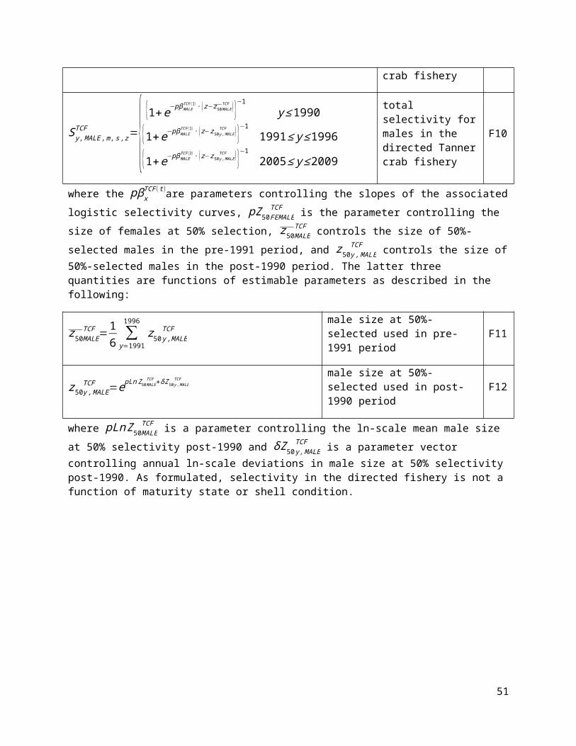
Appendix 2: Equations for a set of pulse fisheries with individual capture, retention and discard mortality probabilities

In the Tanner crab assessment, we are concerned with fitting the retained (Rf) and discarded (Df) components of the total catch (C f =R f +D f ) of Tanner crab on an annual basis in several fisheries (the directed Tanner crab fishery, the snow crab fishery, the Bristol Bay red king crab fishery, and the groundfish fisheries) , as well as accounting for the associated mortality in the population dynamics for the Tanner crab stock. As a clarification of terminology, C f is the total number of crab captured (i.e., brought on board) in fishery f, and Df is the number of crab discarded (i.e. released overboard), not the numbers killed. Unlike many fish species, crabs captured at sea and brought on deck experience little barotrauma and, while some fraction of those subsequently discarded overboard die as a result, the remaining discarded crab survive and continue to contribute to the stock. Experimental lab and observational field studies suggest that discard mortality on Tanner crab captured in the crab fisheries is moderate; we use 50% as the discard mortality fraction for these fisheries. Discard mortality in the groundfish fisheries is assumed to be higher because of gear differences (trawl vs. pot); we use 80% as the discard mortality fraction for Tanner crab in the groundfish fisheries. Total mortality, Mf, of Tanner crab in fishery f is then given by M f =Rf +δ f ∙ D f , where δ f is the discard (i.e., “handling”) mortality fraction in the fishery. So the number of crabs captured by a fishery is more than the number of crabs killed, because discard mortality is not 100%. Because capture, retention and discard processes in the fisheries are sex- and size-dependent, as well as being dependent on shell condition and maturity state, the TCSAM model applies these concepts to individual components of the population (e.g. mature, new shell males between 100 and 105 mm CW) and then sums up the individual contributions to obtain stock-level and fishery-level totals.

For some component (e.g. mature, new shell males between 100 and 110 mm CW) of a population experiencing mortality from several fisheries, the short term change in numbers, N, can be described by the following differential equation:

dNdt

=−(m+∑f

F f ) ∙ N (t ) Rate of change of N over a short period of time 1

where m represents the rate of natural mortality and Ff represents the fishing mortality rate associated with the fth fishery on this component of the population (i.e., Ff includes size-dependent selectivity). The solution to this equation, assuming that m and the Ff’s are constant over the period, is

N (t )=e−( m+FT ) ∙ t ∙N0 Change in N with time 2

where FT=∑f

F f is the rate of total fishing mortality experienced by population component. The

cumulative numbers killed by each fishery, Mf, are described by the equation

d M f

dt=F f ∙ N (t )=F f ∙ e−( m+FT ) ∙t ∙ N0

Rate of change of the numbers killed by fishery f 3

51

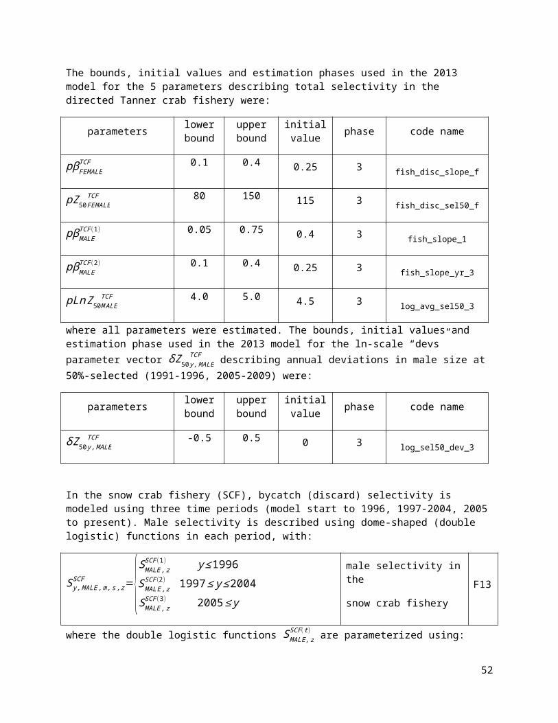
which has the solution

M f (t)=F f

m+ FT∙ [1−e−(m+FT ) ∙ t ] ∙N0 Cumulative numbers killed by fishery f 4

As discussed above, in fisheries that discard part of the catch, and part of that discarded catch may survive, the numbers captured (i.e., brought on board) by the fishery are different from those actually killed by the fishery. Letting ϕ f denote the capture rate associated with fishery f, the cumulative numbers captured in this fishery, Cf, are described by

dC f

dt=ϕf ∙ N=ϕ f ∙ e−( m+FT )∙ t ∙N0

Rate of change of the numbers captured by fishery f 5

which has the solution

C f (t )=ϕ f

m+FT∙ [1−e−(m+F T ) ∙t ] ∙ N0 Numbers captured by fishery f 6

where ϕ f is the fishery capture rate. Of course, C f (t )=Rf ( t )+Df ( t ) (number captured = number retained plus number discarded) and M f (t)=R f (t)+δf ∙ Df (t) (number killed = number retained plus number discarded that die due to handling) for this component of the population.

Letting ρ f denote the fraction of C f ( t ) that is retained, then

R f (t )= ρf ∙C f ( t ) Numbers retained by fishery f 7

and

Df ( t )=(1−ρ f )∙ C f ( t ) Numbers discarded by fishery f 8

so, substituting eq.s 7 and 8 into the equation for M f , one obtains

M f (t)=¿ ρ f ∙C f (t )+δ f ∙(1−ρ f )∙C f (t )M f (t)=¿ [ ρf +δf ∙(1−ρf )] ∙C f ( t )

Numbers killed by fishery f 9

52

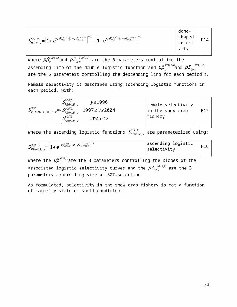
Substituting eq.s 4 and 6 into eq. 9 and eliminating similar terms from both sides, one finds that the fishing mortality rate in the fth fishery is related to the capture rate ϕ f in that fishery by:

F f =[ ρf +δ f ∙ (1−ρf ) ] ∙ ϕ f Fishing mortality rate for fishery f 10

The above equations are based on continuous time models for the fishing and natural mortality processes. To convert these equations to those appropriate for a set of pulse fisheries conducted simultaneously (as used in the Tanner crab model), one takes the limit of the above equations as t →0 and the ϕ f’s gets large

such that ϕ f ∙ t and ϕ f / FT remains constant, for each f. Letting ϕ f ≡ lim

{ t → 0ϕ f → ∞

{ϕ f ∙ t } for all fisheries

simultaneously, one obtains the following equations for a set of pulse fisheries in terms of ϕ f , ρ f , and δ f :

F f =[ ρf +δ f ∙ (1−ρf ) ] ∙ ϕ f fishing mortality rate in fishery f 11

FT=∑f

F f Total fishing mortality rate 12

N+¿=e−FT ∙ N0¿ Population numbers after fisheries 13

C f =ϕ f

FT∙ [1−e−FT ] ∙N 0 Numbers captured in fishery f 14

R f=ρ f ∙C f =ρf ∙ ϕ f

FT∙ [1−e−FT ] ∙ N 0 Numbers retained in fishery f 15

Df =(1−ρf ) ∙ C f=(1− ρf ) ∙ ϕf

FT∙ [1−e−F T ] ∙ N0 Numbers discarded in fishery f 16

M f =Rf +δ f ∙ D f=[ ρ f +δ f ∙(1− ρf )] ∙ C f Total mortality in fishery f 17

DM f=δ f ∙(1−ρf ) ∙C f Discard mortality in fishery f 18

It is important to remember that all terms in eq.s 11-18 apply to individual components of the population, and not the entire population, on an annual basis. The TCSAM models decompose the population by sex, maturity state, shell condition, and size. Thus, each of the quantities above, other than discard mortality δ f (which is assumed to apply equally to all components of the discarded catch), can have additional subscripts x (sex), m (maturity), s (shell condition), z (size) (and y, year, to make the temporal component explicit).

53

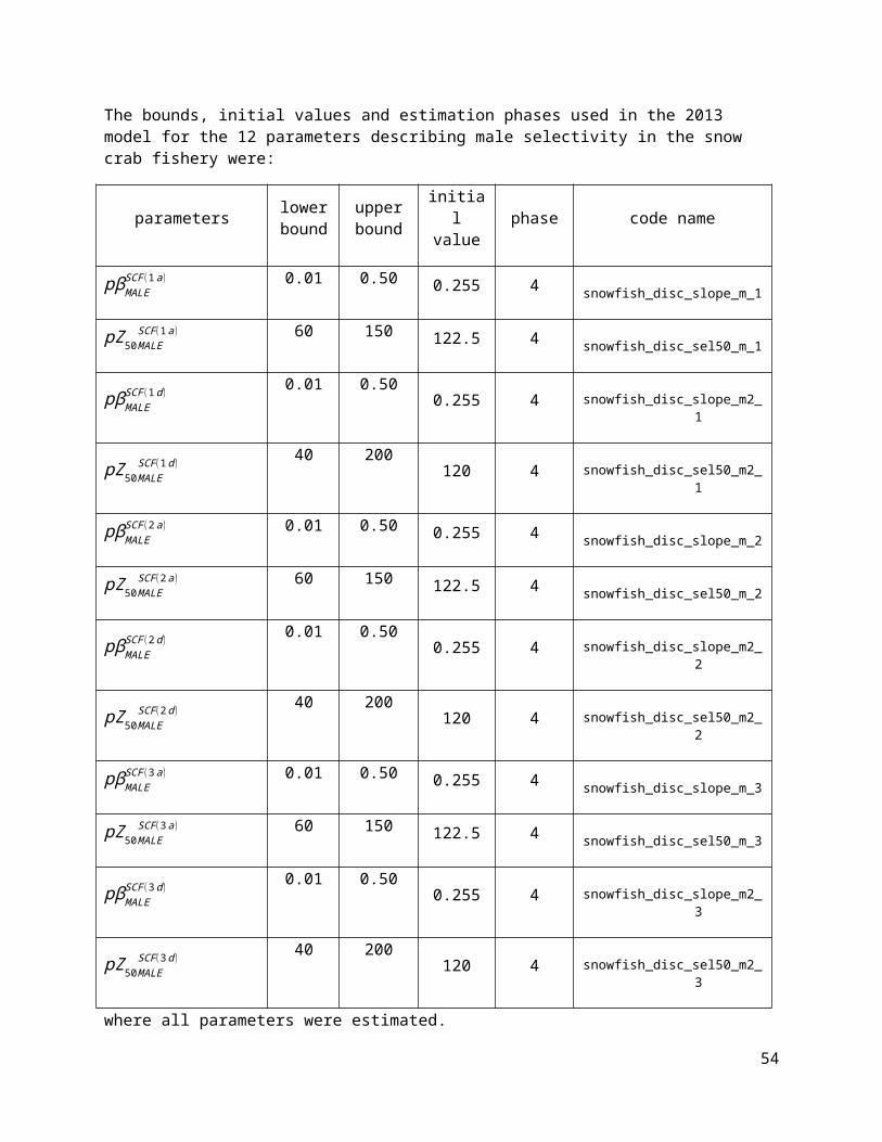
On fitting the TCSAM2103 modelThe TCSAM2013 model is parameterized, in part, based on annual fully-selected fishing mortality rates Ff,y,x,m,s, selectivity functions Sf,y,x,z, and “retention functions” ρ f , y, x , z (the latter non-zero only for males in the directed fishery, of course). The total (size selective) fishing mortality rate is given by

F f , y , x, m, s ,z=F f , y , x, m, s ∙ S f , y , x ,z Total mortality rate (retained+discard) for fishery f 19

from which total annual fishing mortality (in biomass) estimated by the model is compared to the observed total fishing mortality (observed discard biomass discounted by assumed discard mortality added to the retained biomass) in the model’s objective function.

The retained mortality rate in the model is given by

r f , y, x , m,s , z= ρf , y , x , z ∙ F f , y ,x , m,s , z Total retained mortality rate for fishery f 20

However, eq. 15 implies that the retained mortality rate is given by

r f , y, x , m,s , z=ρf , y , x , z ∙ ϕf , y , x ,m, s , z Total retained mortality rate for fishery f 21

Thus the “retention function” ρ f , y, x , z in TCSAM2013 is not equivalent to the retention function ρ f , y, x , z. In fact, ρ f , y, x , z represents the fraction of crab killed in f,y,x,z that were killed due to being retained. This is not equivalent to ρ f , y, x , z, which represents the fraction of crab captured in f,y,x,z that were retained. The latter (ρ f , y, x , z) directly reflects the on-deck sorting process into retained and discards and is independent of handling mortality while the former ( ρ f , y, x , z) only indirectly reflects the on-deck sorting process and actually depends on handling mortality.

The simplest way to see the distinction is to consider a fishery with no discard mortality, so that the only fishing mortality is due to retention. In this case, the retained mortality rate is identical to the fishing mortality rate, so eq. 20 would imply that ρ f , y, x , z ≡1 for this fishery, independent of what the true retention function ρ f , y, x , z is.

However, the overall effect of this difference in terms of model fit and parameter estimation is probably small. It depends on the steepness of the rise of the retention curve ρ f , y, x , z, and is smaller for steeper curves. While not step functions, the retention curves for Tanner crab tend to be fairly steep.

54

Appendix 3: TCSAM2014 DescriptionTo be provided.

55

Executive Summary - North Pacific Fishery … · Web viewF8 where p LnF GTF is a parameter...

Documents

Transcript of Executive Summary - North Pacific Fishery … · Web viewF8 where p LnF GTF is a parameter...