EXCITON DYNAMICS AT PHOTOEXCITED ORGANIC HETEROJUNCTIONS
312
UNIVERSITY OF BELGRADE FACULTY OF PHYSICS Veljko Janković EXCITON DYNAMICS AT PHOTOEXCITED ORGANIC HETEROJUNCTIONS Doctoral Dissertation Belgrade, 2018
Transcript of EXCITON DYNAMICS AT PHOTOEXCITED ORGANIC HETEROJUNCTIONS

UNIVERSITY OF BELGRADE
FACULTY OF PHYSICS
Veljko Janković
EXCITON DYNAMICS AT
PHOTOEXCITED ORGANIC
HETEROJUNCTIONS
Doctoral Dissertation
Belgrade, 2018
UNIVERZITET U BEOGRADU
FIZIQKI FAKULTET
Veko Jankovi
DINAMIKA EKSITONA NA ORGANSKIM
HETEROSPOJEVIMA POBUENIM
SVETLOXU
Doktorska diserta ija
Beograd, 2018
Thesis advisor, Committee member:
Dr Nenad Vukmirović
Research Professor
Institute of Physics Belgrade
University of Belgrade
Committee member:
Prof. Dr Ivanka Milošević
Professor
Faculty of Physics
University of Belgrade
Committee member:
Prof. Dr Ðorđe Spasojević
Associate Professor
Faculty of Physics
University of Belgrade
i

Exciton Dynamics at Photoexcited Organic Heterojunctions
Abstract
The last three decades have seen vigorous and interdisciplinary research activities in the
field of organic photovoltaics. Research efforts in this field are driven by the promise of eco-
nomically viable and environmentally friendly conversion of sunlight into electrical energy at
heterojunctions between an electron-donating (donor) and an electron-accepting (acceptor) or-
ganic material. The light-to-charge conversion in organic solar cells (OSCs) requires the sepa-
ration of the initially photogenerated donor exciton, whose binding energy is much larger than
the thermal energy at room temperature, into free hole and electron in the donor and acceptor
material, respectively. This separation is commonly thought to occur via the electron transfer
from the photoexcited donor to the acceptor material that produces the so-called charge transfer
(CT) exciton, in which the electron and hole are still tightly bound. Despite such large binding
energies of both the donor and CT exciton, experiments on the most efficient OSCs indicate that
virtually all of the photons absorbed by the cell are eventually converted into free carriers in a
process that is weakly aided by both the temperature and the internal electric field in the cell. A
gamut of proposals that could rationalize the aforementioned experimental findings have been
put forward. However, a more detailed understanding of fundamental physical mechanisms that
govern the operation of OSCs on different time scales is still lacking.
The research whose results are presented in this thesis aims to achieve the aforementioned
goal by studying the relevant processes within a relatively simple, yet physically plausible, model
of organic semiconductors and their heterojunctions. Our fully quantum and statistical investiga-
tions of ultrafast dynamics of photoinduced electronic excitations in such models are motivated
by recent experimental results indicating that the light-to-charge conversion in the most efficient
OSCs occurs on subpicosecond time scales. We find that the exciton formation in a neat organic
semiconductor occurs on multiple time scales spanning the range between 50 fs and 1 ps. We
conclude that an overwhelming fraction of spatially separated charges that are present on a 100-
fs time scale after the photoexcitation of a donor/acceptor heterojunction are directly optically
generated from the ground state, and are not obtained as a result of an ultrafast population trans-
fer from donor states. The resonant mixing among donor states and states of spatially separated
ii

charges is at the heart of the direct accessibility of the latter group of states from the ground
state. However, the light absorption still primarily occurs in the donor material, and the charge
separation yields we observe at 1 ps following the excitation suggest that charges predominantly
separate on much longer time scales, starting from the strongly bound donor and CT states. Our
study of charge separation that takes place on long time scales indicates that the combination
of moderate disorder and carrier delocalization can explain quite efficient separation of strongly
bound excitons and its weak dependence on the temperature and electric field.
Keywords: organic photovoltaics, organic semiconductors, exciton, light-to-charge conversion,
charge transfer, charge separation, ultrafast dynamics
Scientific field: Physics
Research area: Condensed matter physics
UDC number: 538.9
iii

Dinamika eksitona na organskim heterospojevima pobuÆenim svetloxu
Saetak
U toku poslede tri de enije sprovode se intenzivna i interdis iplinarna is-
traivaa u oblasti organskih fotovoltaika. Istraivaqki napori u ovoj oblasti
su motivisani mogunoxu ekonomski isplative i ekoloxki prihvative konverz-
ije Sunqeve svetlosti u elektriqnu energiju na heterospojevima dva organska ma-
terijala, od kojih je jedan donor, a drugi ak eptor elektrona. Da bi se izvrxila
konverzija svetlosti u slobodna naelektrisaa u organskim solarnim elijama,
neophodno je razdvojiti ini ijalno generisani donorski eksiton, qija je energija
veze znaqajno vea od termalne energije na sobnoj temperaturi, na slobodne xupinu
i elektron u materijalu donora, odnosno ak eptora. Smatra se da se to razdvajae
obava putem transfera elektrona iz svetloxu pobuÆenog materijala donora u
materijal ak eptora koji vodi stvarau takozvanog ST eksitona (eksitona u ko-
jem je doxlo do transfera naelektrisaa), u kojem su elektron i xupina i dae
jako vezani. Uprkos velikoj vrednosti vezivne energije kako donorskog, tako i ST
eksitona, eksperimenti na najefikasnijim organskim solarnim elijama ukazuju
na to da gotovo svi fotoni apsorbovani u eliji bivaju konvertovani u slobodne
nosio e, pri qemu je ta konverzija slabo potpomognuta kako temperaturom, tako i
unutraxim elektriqnim poem u eliji. Predloeni su mnogobrojni mehanizmi
koji bi mogli da objasne gore pomenute eksperimentalne rezultate. MeÆutim, jox
uvek nedostaje podrobnije razumevae fundamentalnih fiziqkih mehanizama koji
su odgovorni za funk ionisae organskih solarnih elija na razliqitim vremen-
skim skalama.
Istraivae qiji su rezultati prezentovani u ovoj tezi tei da ostvari gore
pomenuti i prouqavajui relevantne pro ese u okvirima relativno jednostavnih,
a fiziqki utemeenih modela organskih poluprovodnika i ihovih heterospojeva.
Naxa u elosti kvantna i statistiqka ispitivaa ultrabrze dinamike svetloxu
generisanih elektronskih eks ita ija u takvim modelima su motivisana nedavnim
eksperimentalnim rezultatima koji ukazuju da se konverzija svetlosti u slobodna
iv

naelektrisaa u najefikasnijim organskim solarnim elijama obava na vremen-
skim skalama ispod jedne pikosekunde. Dobili smo da se formirae eksitona u qis-
tom organskom poluprovodniku obava na vixe razliqitih vremenskih skala koje
se proteu od 50 fs do 1 ps. Zakuqili smo da je najvei deo prostorno razdvojenih
naelektrisaa koja su prisutna na vremenskim skalama reda 100 fs nakon pobude
donor/ak eptor heterospoja direktno optiqki generisan iz osnovnog staa i nije
posledi a ultrabrzog transfera popula ije iz donorskih staa. Mogunost gener-
isaa staa prostorno razdvojenih naelektrisaa direktno iz osnovnog staa je
posledi a ihovog rezonantnog mexaa sa donorskim staima. Ipak, apsorp ija
svetlosti se i dae primarno dexava u materijalu donora, dok prinosi razdva-
jaa naelektrisaa koje opaamo 1 ps nakon pobuÆivaa ukazuju na to da se naelek-
trisaa dominantno razdvajaju na znaqajno duim vremenskim skalama polazei iz
jako vezanih donorskih i ST staa. Naxe ispitivae razdvajaa naelektrisaa
na duim vremenskim skalama pokazuje da kombina ija umerene neureÆenosti i de-
lokaliza ije nosila a moe da objasni veoma efikasno razdvajae jako vezanih
eksitona i egovu slabu zavisnost od temperature i elektriqnog poa.
Kuqne reqi: organski fotovoltai i, organski poluprovodni i, eksiton, kon-
verzija svetlosti u naelektrisaa, transfer naelektrisaa, razdvajae naelek-
trisaa, ultrabrza dinamika
Nauqna oblast: Fizika
Oblast istraivaa: Fizika kondenzovane materije
UDK broj: 538.9
v
Acknowledgements
The research whose results are presented in this thesis has been entirely conducted in the Sci-
entific Computing Laboratory (SCL) of the Institute of Physics Belgrade (IPB). The research
project has been supervised by Dr Nenad Vukmirović, Research Professor at IPB. It was a great
honor and an immense pleasure to enter the world of science under the guidance of Dr Vuk-
mirović. After our fruitful collaboration during my master programme, Dr Vukmirović has of-
fered me the opportunity to work with him on, at that time, extremely hot topic of free-charge
generation in organic solar cells based on a heterojunction between two organic semiconduc-
tors. However, instead of performing ab initio calculations and obtaining quantitative insights
on particular material systems, he suggested that the problem be tackled from a physicists’ per-
spective. In the last four years, step by step, we have been building our own view of free-charge
generation in organic solar cells, which has ultimately resulted in the publication of this thesis.
I am deeply indebted to Dr Vukmirović for his generous help and patience during our collabora-
tion. He has been extremely dedicated to pursuing the new research line that was launched with
the start of my doctoral programme. He was always open to thorough discussions on different
aspects of problems and difficulties that I encountered during my research. However, he did his
best to keep my focus on the aspects that were really relevant for the topic we worked on. Dr
Vukmirović has also invested a great deal of effort in finding viable ways of communicating our
results to the global scientific community. Thanks to his Marie Curie Integration Grant and his
active participation in the COST Action MultiscaleSolar, I had many opportunities to proudly
present our findings at scientific conferences all over Europe. I appreciate very much his efforts
to create a specific research climate that was supposed to mimic the one found in world’s leading
research institutions. I very much hope that the future will show that all these efforts have not
been in vain.
I am also grateful to Dr Antun Balaž for giving me the opportunity to be part of SCL and
participate in the National Project ON171017 Modeling and Numerical Simulations of Complex
Many-Particle Systems. I would also like to acknowledge continuous support and encouragement
that I have received from Dr Balaž during all these years. Despite his numerous duties, he has
vi

always been willing to discuss with me various problems and dilemmas that I have encountered
both on professional and personal level. Certain pieces of his advice, which stem from his broad
life experience, have made a strong impact on me and on my attitude towards a carrier in science
and life in general.
My work in SCL would not have been so pleasant if I had not been surrounded by very kind
and helpful colleagues. The implementation of the equations I derived into working computa-
tional codes on high performance computing architectures would not have been possible without
generous assistance of the ICT staff. In particular, I give thanks to Mr Petar Jovanović for his
help in writing codes that can be run on the PARADOX Supercomputing Facility and for his
invaluable advice concerning programming and information technologies in general.
During my doctoral programme, I was also involved in teaching at the Faculty of Physics as
an external collaborator. I would like to thank all the people who supported my inclusion in the
teaching process at the Faculty, in particular Prof. Dr Sunčica Elezović-Hadžić, Doc. Dr Duško
Latas, Prof. Dr Zoran Radović, and Doc. Dr Mihajlo Vanević. I enjoyed the collaboration
with Dr Vanević and Prof. Radović on teaching Quantum Statistical Physics. Their sugges-
tions have helped me maintain balance between research and teaching activities, while thorough
discussions with them have greatly impacted my view of research and science. Despite being
relatively infrequent, conversations with Prof. Elezović-Hadžić have always been reassuring and
full of support and understanding.
I cannot help mentioning my activities in the National Committee for High-School Physics
Competitions, in which I participated as one of the authors of problems offered to the final-year
students. Let me thank my coauthors, Dr Vukmirović and Ms Ana Hudomal, for very nice and
fertile cooperation in preparing problems for all levels of the competition cycle. My work in
the Committee was very rewarding because I had the opportunity to broaden my understand-
ing of some basic physical phenomena, learn how science should be communicated to young
generations, and make contacts with brilliant young minds that are bound to become renowned
experts in the future. I had numerous opportunities to informally discuss with the President
of the Committee, Doc. Dr Božidar Nikolić, who taught me many lessons that are not part of
standard university curricula by sharing his rich experience in both teaching and research.
vii
In the end, let me thank my mother Gordana for putting up with me during all these years
and for providing me with unconditional love and support. Even though her expertise lies well
outside research and science, she has always been at my disposal and ready to help me evalu-
ate my own achievements and assess their position in a broader context. I firmly believe that
her participation in my continuous self-evaluation has played an important role in my doctoral
programme.
The research activities conducted during my doctoral studies were supported by the Ministry
of Education, Science, and Technological Development of the Republic of Serbia (Project No.
ON171017), the European Community FP7 Marie Curie Integration Grant ELECTROMAT,
and the European Commission under H2020 project VI-SEEM, Grant No. 675121. I have also
benefited from the contribution of the COST Action MP1406 (MultiscaleSolar).
viii

Contents
Members of the Thesis Defense Committee i
Abstract ii
Abstract in Serbian iv
Acknowledgements vi
List of Figures xiii
List of Tables xvii
List of Abbreviations xviii
Physical Constants xx
List of Symbols xxi
1 Introduction 1
1.1 Global Energy Issue . . . . . . . . . . . . . . . . . . . . . . . . . . . . . . . . 1
1.2 Photovoltaic Effect and Solar Cell . . . . . . . . . . . . . . . . . . . . . . . . 3
1.3 Organic Semiconductors . . . . . . . . . . . . . . . . . . . . . . . . . . . . . 6
1.3.1 Electronic Configuration of Carbon in Organic Semiconductors . . . . 7
1.3.2 Different Types of Organic Semiconductors . . . . . . . . . . . . . . . 10
1.3.3 Comparison between Inorganic and Organic Semiconductors . . . . . . 16
1.4 Organic Solar Cells . . . . . . . . . . . . . . . . . . . . . . . . . . . . . . . . 18
1.5 Critical View of the Sequential Mechanism of OSC Operation . . . . . . . . . 23
ix

1.6 Organization of the Thesis . . . . . . . . . . . . . . . . . . . . . . . . . . . . 28
2 Standard Semiconductor Model 32
2.1 Two-Band Semiconductor Model . . . . . . . . . . . . . . . . . . . . . . . . . 33
2.2 Definition of Exciton . . . . . . . . . . . . . . . . . . . . . . . . . . . . . . . 42
2.3 Wannier and Frenkel Exciton Models . . . . . . . . . . . . . . . . . . . . . . . 45
2.3.1 Wannier Exciton Model . . . . . . . . . . . . . . . . . . . . . . . . . 46
2.3.2 Frenkel Exciton Model . . . . . . . . . . . . . . . . . . . . . . . . . . 50
3 Theoretical Approach to Ultrafast Exciton Dynamics 55
3.1 General Picture of the Dynamics of Photoexcited Semiconductors . . . . . . . 56
3.2 Density Matrix Theory . . . . . . . . . . . . . . . . . . . . . . . . . . . . . . 57
3.3 Brief Review of Theoretical Approaches to Ultrafast Exciton Dynamics . . . . 59
3.4 Fundamentals of the DCT Scheme . . . . . . . . . . . . . . . . . . . . . . . . 62
3.5 The DCT Scheme up to the Second Order in Applied Field . . . . . . . . . . . 68
3.5.1 Energy and Particle-Number Conservation . . . . . . . . . . . . . . . 75
3.5.2 Closing the Phonon Branch of the Hierarchy . . . . . . . . . . . . . . 76
3.5.3 Another View of the Second-Order Semiconductor Dynamics . . . . . 82
3.5.4 Schematic Picture of the Second-Order Semiconductor Dynamics . . . 84
Coherent and Incoherent Quantities . . . . . . . . . . . . . . . . . . . 84
Analysis of the Semiconductor Dynamics . . . . . . . . . . . . . . . . 87
4 Ultrafast Exciton Dynamics in Photoexcited Neat Semiconductors 89
4.1 Theoretical and Experimental Background . . . . . . . . . . . . . . . . . . . . 89
4.2 Model Description . . . . . . . . . . . . . . . . . . . . . . . . . . . . . . . . 93
4.2.1 One-Dimensional Semiconductor Model . . . . . . . . . . . . . . . . 93
4.2.2 Parametrization of the Model Hamiltonian . . . . . . . . . . . . . . . . 96
4.3 Numerical Results . . . . . . . . . . . . . . . . . . . . . . . . . . . . . . . . . 99
4.3.1 Organic Set of Parameters . . . . . . . . . . . . . . . . . . . . . . . . 102
4.3.2 Inorganic Set of Parameters . . . . . . . . . . . . . . . . . . . . . . . 111
x

4.4 Discussion and Significance of Our Results . . . . . . . . . . . . . . . . . . . 114
5 Origin of Ultrafast Charge Separation 116
5.1 Experimental and Theoretical Background . . . . . . . . . . . . . . . . . . . . 116
5.1.1 Overview of Recent Experimental Results . . . . . . . . . . . . . . . . 117
5.1.2 Overview of Recent Theoretical Results . . . . . . . . . . . . . . . . . 121
5.2 Model Description . . . . . . . . . . . . . . . . . . . . . . . . . . . . . . . . 124
5.2.1 One-Dimensional Lattice Model of a Heterojunction . . . . . . . . . . 124
5.2.2 Parametrization of the Model Hamiltonian . . . . . . . . . . . . . . . . 127
5.2.3 Classification of Exciton States . . . . . . . . . . . . . . . . . . . . . . 131
5.3 Numerical Results . . . . . . . . . . . . . . . . . . . . . . . . . . . . . . . . . 133
5.3.1 Interfacial Dynamics on Ultrafast Time Scales . . . . . . . . . . . . . 134
5.3.2 Impact of Model Parameters on Ultrafast Exciton Dynamics . . . . . . 136
5.4 Ultrafast Spectroscopy Signatures . . . . . . . . . . . . . . . . . . . . . . . . 142
5.4.1 Basics of Ultrafast Transient Absorption Spectroscopy and Conventional
Interpretation of Experimental Signals . . . . . . . . . . . . . . . . . . 143
5.4.2 Theoretical Treatment of Ultrafast Transient Absorption Spectroscopy . 145
5.4.3 Numerical Results: Ultrafast Differential Transmission Signals . . . . . 151
5.5 Discussion and Significance of Our Results . . . . . . . . . . . . . . . . . . . 155
6 Identification of Ultrafast Photophysical Pathways 159
6.1 Motivation . . . . . . . . . . . . . . . . . . . . . . . . . . . . . . . . . . . . . 159
6.2 Model Description . . . . . . . . . . . . . . . . . . . . . . . . . . . . . . . . 162
6.2.1 Multiband Model Hamiltonian of a Heterojunction . . . . . . . . . . . 162
6.2.2 Parameterization of the Model Hamiltonian . . . . . . . . . . . . . . . 164
6.2.3 Role of the D/A Coupling and the Resonant Mixing Mechanism . . . . 168
6.3 Numerical Results . . . . . . . . . . . . . . . . . . . . . . . . . . . . . . . . . 174
6.3.1 General Analysis of Ultrafast Interfacial Dynamics . . . . . . . . . . . 176
6.3.2 Individuation of Ultrafast Photophysical Pathways . . . . . . . . . . . 180
6.3.3 Influence of Model Parameters on Ultrafast Exciton Dynamics . . . . . 184
xi

6.4 Discussion and Significance of Our Results . . . . . . . . . . . . . . . . . . . 192
7 Incoherent Charge Separation at Photoexcited Organic Bilayers 195
7.1 Solar Cells as Electric Devices . . . . . . . . . . . . . . . . . . . . . . . . . . 195
7.2 Experimental and Theoretical Background . . . . . . . . . . . . . . . . . . . . 198
7.2.1 Overview of Recent Experimental Results . . . . . . . . . . . . . . . . 198
7.2.2 Overview of Recent Theoretical Results . . . . . . . . . . . . . . . . . 201
7.3 Model and Method . . . . . . . . . . . . . . . . . . . . . . . . . . . . . . . . 205
7.3.1 Model Hamiltonian . . . . . . . . . . . . . . . . . . . . . . . . . . . . 205
7.3.2 Theoretical Approach to Incoherent Charge Separation . . . . . . . . . 207
7.3.3 Parameterization of the Model Hamiltonian . . . . . . . . . . . . . . . 210
7.4 Numerical Results . . . . . . . . . . . . . . . . . . . . . . . . . . . . . . . . . 216
7.4.1 Charge Separation from the Strongly Bound CT State . . . . . . . . . . 218
7.4.2 Charge Separation from a Donor Exciton State . . . . . . . . . . . . . 231
7.5 Discussion and Significance of Our Results . . . . . . . . . . . . . . . . . . . 238
8 Conclusion 242
A Proofs of the Expansion and Truncation Theorems in the Phonon-Free Case 247
A.1 Proof of the Expansion Theorem . . . . . . . . . . . . . . . . . . . . . . . . . 247
A.2 Proof of the Truncation Theorem . . . . . . . . . . . . . . . . . . . . . . . . . 249
B Contraction Relations Relevant for the Second-Order Dynamics 251
C Markov and Adiabatic Approximations 254
D Further Details about Closing the Hierarchy of Equations 256
D.1 Closing the Phonon Branch of the Hierarchy . . . . . . . . . . . . . . . . . . . 256
D.2 Comments on the Energy Conservation . . . . . . . . . . . . . . . . . . . . . 258
Curriculum Vitae–Veljko Janković 281
xii

List of Figures
1.1 Fuel shares of the total primary energy supply in 1973 and 2015. . . . . . . . . 2
1.2 General scheme of a solar cell. . . . . . . . . . . . . . . . . . . . . . . . . . . 3
1.3 Benzene molecule and its π-electron molecular orbitals. Series of oligoacenes.
Crystal structure of pentacene molecular crystal. . . . . . . . . . . . . . . . . . 9
1.4 Molecular orbitals of two isolated molecules and their dimer. . . . . . . . . . . 11
1.5 Chemical formulae of fullerene and PCBM molecules. . . . . . . . . . . . . . 12
1.6 Structure of trans-polyacetylene and Peierls instability. . . . . . . . . . . . . . 13
1.7 Chemical formulae of monomer units of P3HT and PCPDTBT polymers. Unit
cell of the ideally ordered P3HT polymer. . . . . . . . . . . . . . . . . . . . . 15
1.8 Schematic view of active layers of different types of OSCs. . . . . . . . . . . . 19
1.9 Band alignment in a D/A OSC. . . . . . . . . . . . . . . . . . . . . . . . . . . 19
1.10 Pictorial view of the sequential mechanism of light-to-charge conversion in OSCs. 21
1.11 Pictorial view of “hot” and “cold” charge separation mechanisms in OSCs. . . . 27
3.1 Schematic picture of the hierarchy of equations for density matrices. . . . . . . 82
4.1 Schematic view of the parallelization scheme implemented in our own C pro-
gram that performs integration of the system of quantum kinetic equations. . . . 101
4.2 Exciton spectrum in the model of a neat organic semiconductor. . . . . . . . . 103
4.3 Time evolution of the number of bound excitons in the model of a neat organic
semiconductor for different central frequencies of the excitation. . . . . . . . . 105
4.4 Time evolution of the number of bound excitons in the model of a neat organic
semiconductor for different temperatures. . . . . . . . . . . . . . . . . . . . . 106
xiii

4.5 Time evolution of exciton populations in particular exciton bands in the model
of a neat organic semiconductor for different temperatures. . . . . . . . . . . . 107
4.6 Time evolution of the number of coherent excitons for different temperatures. . 107
4.7 Time evolution of the number of bound excitons in the model of a neat organic
semiconductor for different carrier-phonon interaction strengths. . . . . . . . . 108
4.8 Time evolution of the number of bound excitons in the model of a neat organic
semiconductor for different values of the on-site Coulomb interaction. . . . . . 109
4.9 Exciton spectrum in the model of a neat inorganic semiconductor. . . . . . . . 111
4.10 Exciton dynamics in the model of a neat inorganic semiconductor. . . . . . . . 113
5.1 Schematic view of ultrafast optical experiments performed by Bakulin et al. [48]. 118
5.2 Schematic view of ultrafast optical experiments performed by Jailaubekov et
al. [37]. . . . . . . . . . . . . . . . . . . . . . . . . . . . . . . . . . . . . . . 119
5.3 Schematic view of ultrafast optical experiments performed by Grancini et al. [36].120
5.4 Schematic view of the two-band model of a D/A heterojunction. . . . . . . . . 125
5.5 Time evolution of populations of various groups of exciton states, together with
the probability of an electron being in the acceptor, in the two-band model of a
D/A heterojunction. . . . . . . . . . . . . . . . . . . . . . . . . . . . . . . . . 135
5.6 Ultrafast exciton dynamics in the two-band model of a D/A heterojunction for
different values of the D/A electronic coupling. . . . . . . . . . . . . . . . . . 137
5.7 Ultrafast exciton dynamics in the two-band model of a D/A heterojunction for
different values of the LUMO–LUMO offset. . . . . . . . . . . . . . . . . . . 138
5.8 Ultrafast exciton dynamics in the two-band model of a D/A heterojunction for
different values of the electronic coupling in the acceptor. . . . . . . . . . . . . 138
5.9 Ultrafast exciton dynamics in the two-band model of a D/A heterojunction for
different carrier–phonon interaction strengths. . . . . . . . . . . . . . . . . . . 139
5.10 Ultrafast exciton dynamics in the two-band model of a D/A heterojunction for
different ratios of the carrier–phonon coupling constants with high- and low-
frequency phonon modes. . . . . . . . . . . . . . . . . . . . . . . . . . . . . . 141
xiv

5.11 Ultrafast exciton dynamics in the two-band model of a D/A heterojunction for
different temperatures. . . . . . . . . . . . . . . . . . . . . . . . . . . . . . . 142
5.12 Principal scheme of an ultrafast time-resolved TA spectroscopy experiment. . . 144
5.13 Time evolution of theoretical DTSs emerging from our dynamics for different
wave lengths of pump and probe pulses. . . . . . . . . . . . . . . . . . . . . . 153
6.1 Schematic view of the multiband model of a D/A heterojunction. . . . . . . . . 166
6.2 Schematic view of the classification of exciton states in the model of a D/A
heterojunction. . . . . . . . . . . . . . . . . . . . . . . . . . . . . . . . . . . 170
6.3 Exciton spectrum and ultrafast photophysical pathways in the multiband model
of a D/A heterojunction. . . . . . . . . . . . . . . . . . . . . . . . . . . . . . 173
6.4 Time evolution of populations of various groups of exciton states in the multi-
band and two-band model of a D/A heterojunction. . . . . . . . . . . . . . . . 177
6.5 Time- and energy-resolved numbers of coherent excitons in various groups of
exciton states in the multiband model of a D/A heterojunction. . . . . . . . . . 179
6.6 Time- and energy-resolved numbers of excitons in various groups of exciton
states in the multiband model of a D/A heterojunction. . . . . . . . . . . . . . 181
6.7 Electron and hole distributions in representative exciton states participating in
the ultrafast dynamics of the multiband model of a D/A heterojunction. . . . . . 183
6.8 Ultrafast exciton dynamics in the multiband model of a D/A heterojunction for
different central frequencies of the excitation. . . . . . . . . . . . . . . . . . . 185
6.9 Influence of small variations in the LUMO–LUMO offset on the ultrafast exciton
dynamics in the multiband model of a D/A heterojunction. . . . . . . . . . . . 187
6.10 Ultrafast exciton dynamics in the multiband model of a D/A heterojunction for
different carrier–phonon interaction strengths. . . . . . . . . . . . . . . . . . . 188
6.11 Time- and energy-resolved numbers of excitons is various groups of exciton
states for different strengths of the carrier–phonon interaction in the multiband
model of a D/A heterojunction. . . . . . . . . . . . . . . . . . . . . . . . . . . 190
xv

7.1 Electron energy levels relevant for the operation of an OSC under different work-
ing conditions. . . . . . . . . . . . . . . . . . . . . . . . . . . . . . . . . . . . 196
7.2 Current-voltage characteristic of a solar cell in the dark and under illumination. 198
7.3 Schematic view of the model of a D/A bilayer. . . . . . . . . . . . . . . . . . . 211
7.4 Disorder-averaged densities of states for various groups of exciton states. . . . . 216
7.5 Field-dependent yield of charge separation from the strongly bound CT state.
Relative position of the low-energy edges of the densities of CT and contact
exciton states. . . . . . . . . . . . . . . . . . . . . . . . . . . . . . . . . . . . 219
7.6 Distributions of the yield of charge separation from the strongly bound CT state
for different strengths of the electric field. . . . . . . . . . . . . . . . . . . . . 220
7.7 Distribution of energies of the intermediate and initial CT state. . . . . . . . . . 223
7.8 Yield of charge separation from the strongly bound CT state as a function of the
disorder strength. Disorder-averaged energy barrier opposing the separation of
the strongly bound CT state as a function of the disorder strength. . . . . . . . 226
7.9 Field-dependent separation yield from the strongly bound CT state for different
degrees of carrier delocalization and Coulomb interaction strengths. . . . . . . 228
7.10 Yield of charge separation from the strongly bound CT state as a function of the
temperature and LUMO–LUMO offset. . . . . . . . . . . . . . . . . . . . . . 229
7.11 Field-dependent yield of charge separation starting from donor exciton states of
different energies. . . . . . . . . . . . . . . . . . . . . . . . . . . . . . . . . . 232
7.12 Yield of the donor exciton separation as a function of the disorder strength. . . 234
7.13 Field-dependent separation yield from the closely separated donor state for dif-
ferent degrees of carrier delocalization and Coulomb interaction strengths. . . . 236
7.14 Yield of the separation from the closely separated donor state as a function of
the temperature and LUMO–LUMO offset. . . . . . . . . . . . . . . . . . . . 236
xvi

List of Tables
4.1 Values of model parameters used in computations on the model of a neat semi-
conductor. . . . . . . . . . . . . . . . . . . . . . . . . . . . . . . . . . . . . . 98
4.2 Active density matrices, their total numbers in the most general case and the
case specific to our model. . . . . . . . . . . . . . . . . . . . . . . . . . . . . 99
5.1 Values of model parameters used in computations on the two-band model of a
D/A heterojunction. . . . . . . . . . . . . . . . . . . . . . . . . . . . . . . . . 128
6.1 Values of model parameters used in computations on the multiband model of a
D/A heterojunction. . . . . . . . . . . . . . . . . . . . . . . . . . . . . . . . . 165
7.1 Values of model parameters used in computations on the model of a D/A bilayer. 213
xvii

List of Abbreviations
PCE power conversion efficiency
IQE internal quantum efficiency
OSC organic solar cell
OPV organic photovoltaic
LUMO lowest unoccupied molecular orbital
HOMO highest occupied molecular orbital
D/A donor/acceptor
PCBM [6,6]-phenyl-C61 butyric acid methyl ester
P3HT poly(3-hexylthiophene)
PCPDTBT poly[2,6-(4,4-bis-(2-ethylhexyl)-4H-cyclopenta [2,1-b;3,4-b’] dithiophene)-
-alt-4,7(2,1,3-benzothiadiazole)]
CT charge transfer (state, exciton)
CS charge separated (state, exciton)
DCT dynamics controlled truncation (scheme)
TA transient absorption (spectroscopy, experiment)
DTS differential transmission signal
VB valence band
CB conduction band
SBE semiconductor Bloch equation
TR-FU time-resolved fluorescence up-conversion
NLO nonlinear optical (crystal)
LAPACK Linear Algebra Package
HPC high performance computing
xviii

MPI Message Passing Interface
(TR-)SHG (time-resolved) second harmonic generation
XD donor exciton (state)
XA acceptor exciton (state)
GSB ground state bleaching
SE stimulated emission
PIA photoinduced absorption
kMC kinetic Monte Carlo
xix
Physical Constants
Elementary Charge e = 1.602× 10⁻¹⁹C
Vacuum Permittivity ε0 = 8.854× 10⁻¹² Fm−1
Electron Mass me = 9.109× 10⁻³¹ kg
Boltzmann Constant kB = 1.380× 10⁻²³ JK−1
Vacuum Permeability µ0 = 4π × 10−7TmA−1
xx
List of Symbols
εr relative dielectric permittivity
rCT electron–hole separation in the “cold” CT exciton
ǫCTb binding energy of the “cold” CT exciton
Ψ (r)[Ψ† (r)
]Fermi field operators annihilating [creating] a particle in r
bµ[b†µ]
Bose operators annihilating [creating] a phonon in mode µ
~ωµ energy of phonon mode µ
E(t), E(t), E external electric field
ap[a†p]
Fermi operators annihilating [creating] a particle in single-particle state p
Eg semiconductor single-particle gap
cp[c†p]
Fermi operators annihilating [creating] an electron in conduction-band state p ∈ CB
dp[d†p]
Fermi operators annihilating [creating] a hole in valence-band state p ∈ VB
ǫcp [ǫvp] energy of conduction-band state p ∈ CB [valence-band state p ∈ VB]
Vλpλqλkλl
pqkl matrix element of the Coulomb interaction in the electron–hole picture
γµpq matrix element of the carrier-phonon interaction in the electron–hole picture
Mλpλqpq matrix element of the dipole-moment operator in the electron–hole picture
|0〉e vacuum state in the particle picture
|GS〉 semiconductor ground state in the particle picture
|0〉 semiconductor ground state in the electron–hole picture
|x〉 exciton state x (eigenstate x of an electron–hole pair)
~ωx energy of exciton state x
Xx
[X†
x
]operators annihilating [creating] an exciton in state x
ψxab exciton “wavefunction”, i.e., scalar product 〈ab|x〉 (a ∈ VB, b ∈ CB)
m∗e (m∗
h) electron (hole) effective mass
xxi

ǫXb binding energy of the Wannier exciton (K = 0, n = 1)
a0,X electron–hole separation in the Wannier exciton (K = 0, n = 1)
Yab interband polarizations in the single-particle basis
Cab (Dab) electron (hole) populations and intraband polarizations in the single-particle basis
Ne electron number operator
Ne electron number
Nh hole number operator
Nh hole number
Ntot total exciton number
Nabcd exciton populations and exciton–exciton coherences in the single-particle basis
yx interband polarizations in the exciton basis
yxµ± single-phonon-assisted interband polarizations in the exciton basis
nxx exciton populations and exciton–exciton coherences in the exciton basis
nxxµ+ single-phonon-assisted exciton populations and exciton–exciton coherences
in the exciton basis
nxx incoherent part of exciton populations and exciton–exciton coherences
in the exciton basis
Mx, Mx matrix elements of the dipole-moment operator in the exciton basis
Γµxx, Γiλi
xx matrix elements of the carrier–phonon interaction in the exciton basis
nphµ
[nph(E)
]equilibrium number of phonons in phonon mode µ [of energy E]
T temperature
U on-site Coulomb interaction
ǫpolb polaron binding energy
ωc central frequency of the excitation
F vector of the internal electric field in the cell
xxii

To my childhood and my youth
To the only one that has never abandoned me
xxiii

Chapter 1
Introduction
1.1 Global Energy Issue
Finding economically viable and efficient ways of utilizing renewable resources of energy to
satisfy an ever-increasing global energy demand is one of the major challenges of the 21st century.
According to the definition provided by the International Energy Agency [1],
“Renewable energy is derived from natural processes that are replenished constantly. In its var-
ious forms, it derives directly from the Sun, or from heat generated deep within the Earth. In-
cluded in the definition is electricity and heat generated from solar, wind, ocean, hydropower,
biomass, geothermal resources, and biofuels and hydrogen derived from renewable resources.”
The amount of energy produced during one year on the global level, as measured by the
world total primary energy supply, has more than doubled in the last forty years, rising from ca.
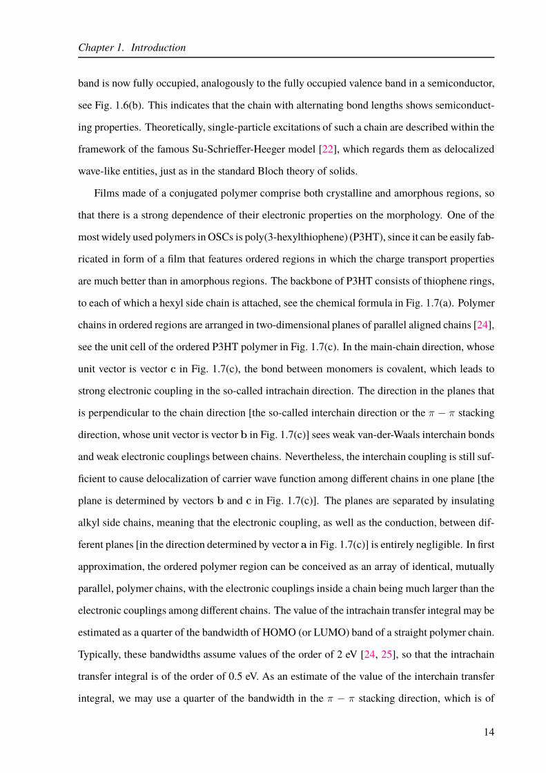
70,000 TWh in 1973 to ca. 160,000 TWh in 2015 [2]. The largest part of the energy is generated
by using fossil fuels, such as oil, coal, and natural gas, see the fuel shares of the total primary
energy supply in Fig. 1.1. These resources of energy are limited, unevenly distributed, and cause
excessive emissions of CO2 in the Earth’s atmosphere, thus promoting the global warming. The
participation of the energy generated from fossil fuels in the total produced energy has somewhat
decreased (from 86.7% in 1973 to 81.4% in 2015, see Fig. 1.1), mainly due to an increase in the
contribution of the nuclear energy. At the same time, the share of the energy from all renewable
resources has risen from 0.1% in 1973 to 1.5% in 2015. The nuclear energy, however, cannot be
1

Chapter 1. Introduction
Coa
l (24
.5%
)
Oil (4
6.2%
)
Nat
ural g
as (1
6.0%
)
Nuc
lear
(0.9
%)
Hyd
ro (1
.8%
)
Biofu
els an
d was
te (1
0.5%
)
Oth
er (0
.1%
)
Coa
l (28
.1%
)
Oil (3
1.7%
)
Nat
ural g
as (2
1.6%
)
Nuc
lear
(4.9
%)
Hyd
ro (2
.5%
)
Biofu
els an
d was
te (9
.7%
)
Oth
er (1
.5%
)0
10
20
30
40
50
1973 2015
Pe
rce
ntu
al fu
el sh
are
s
Pe
rce
ntu
al fu
el sh
are
s
0
10
20
30
40
50
Figure 1.1: Fuel shares of the total primary energy supply in 1973 and 2015. Theresources denoted by “Other” include geothermal, solar, wind, ocean, and otherresources. The data are extracted from Ref. [2].
regarded as a sustainable solution to the global energy problem because of the risks related to
the operation of nuclear power plants, the issue of the nuclear waste, and the latent threat of its
military use. Having in mind the predicted growth of both the global population and the average
income in the near future, as well as the fact that the fossil fuels are slowly but surely running out,
a sustainable and long-term solution to the global energy problem has to be formulated. To this
end, governments and companies throughout the world are providing more and more funding for
fundamental and applied research that would lead to a large-scale and cost-effective exploitation
of the energy from renewable resources.
Among all of the renewable energy resources, the energy of the Sun, together with the wind
energy, has the greatest theoretical potential to resolve the global energy issue. To understand
this, it is enough to remember that the intensity of the orthogonally incident solar radiation
just outside the Earth atmosphere is approximately 1.36 kW/m2 (the so-called solar constant).
Remembering that the solar power reaching the Earth is distributed over the illuminated Earth
hemisphere, and that every point on the surface of the Earth is, on average, illuminated for 12
hours every day, one can calculate that, on average and disregarding the influence of the Earth
atmosphere, each square meter of the Earth receives the solar power of 340 W [3]. The total
energy that we receive from the Sun during one year is approximately 1.5 × 10⁹ TWh, which is
around 10,000 times larger than the global annual energy consumption in 2015 [2].
2

Chapter 1. Introduction
Figure 1.2: General scheme of a solar cell. HSC stands for the hole-selective con-tact, in which the hole conductivity σp is much larger than the electron conductivityσn. ESC stands for the electron-selective contact, in which the inequality σn ≫ σpholds. The solid (dashed) horizontal lines in the HSC, active layer, and ESC, aremeant to represent the edges of the conduction (valence) band. The dashed verticalarrow in the active layer represents the light absorption generating electrons (fullcircles) in the conduction band and holes (empty circles) in the valence band.
1.2 Photovoltaic Effect and Solar Cell
The conversion of solar energy to electricity is based on the photovoltaic effect whose discovery
in 1839 is commonly attributed to Alexandre-Edmond Becquerel [4]. In essence, the photo-
voltaic effect is a physical and chemical phenomenon consisting of the creation of voltage and
electric current in a material upon its irradiation by light. Solar cells (or photovoltaic cells)
are electric devices that convert sunlight into electricity by means of the photovoltaic effect. A
solar cell typically consists of the active layer (usually made of a semiconductor material) that
is sandwiched between two carrier-selective contacts. The material constituting the active layer
can absorb light and convert the energy of the photons absorbed into excess carriers, whose num-
ber is determined by the competition between the rates of their generation and recombination.
A very general scheme of a solar cell is presented in Fig. 1.2. The basic features of the solar cell
operation mechanism are:
(a) the absorption of light of sufficient energy by a semiconductor material promotes an elec-
tron from the valence band to the conduction band, leaves a hole in the valence band, and
3
Chapter 1. Introduction
generates an electron–hole pair (exciton);
(b) the oppositely charged electron and hole thus generated are separated, either spontaneously
or by some other means;
(c) the separated charge carriers should be separately extracted at the carrier-selective contacts
and can then be used to generate photocurrent in the external circuit.
The aforementioned carrier-selectivity of the contacts is crucial to the production of the pho-
tocurrent [5]. An electron-selective contact is permeable for electrons and blocks the holes,
i.e., it is a good conductor of electrons and a poor conductor of holes. On the other hand, a
hole-selective contact is impermeable for electrons, i.e., it has a large conductivity for holes
and a small conductivity for electrons. Typical electron-selective contact is made of an n-type
semiconductor, whereas p-type semiconductors are used as hole-selective contacts. In order to
prevent hole (electron) injection from the absorber into the electron-selective (hole-selective)
contact, the energy band gaps of the contacts are generally larger than the energy band gap of
the active layer. The contacts, therefore, transmit almost all of the incident photons, which are
then absorbed in the active layer. Metal contacts, by means of which the carriers are finally
extracted to the external circuit, are in contact with carrier-selective layers.
There are numerous ways to quantify the performance of a solar cell (see, e.g., Ch. 4 of
Ref. [6]). The solar cell efficiency may be assessed by computing the so-called power conversion
efficiency (PCE), which is given by the ratio of the maximum electrical power delivered by the
solar cell per unit device area and the intensity of the incident light (i.e., the light power incident
onto the unit device area)
PCE =electrical power delivered
incident light power. (1.1)
The PCE of a solar cell is directly relevant for applications, in which the solar cell delivers power
to the external load by maintaining its ends at different electric potentials and forcing the electric
current through it. For scientific analyses, other figures of merit may be more useful. Let us here
introduce the so-called internal quantum efficiency (IQE) of the solar cell, which quantifies the
4

Chapter 1. Introduction
efficiency with which the photons absorbed by the active layer are converted into free charges
capable of producing photocurrent. Differently from the PCE, the IQE is measured under the
so-called short-circuit conditions, when the voltage (and consequently the power) delivered by
the solar cell is equal to zero. Formally, the IQE is the ratio of the electron flux in the circuit (the
number of electrons obtained per unit device area and per unit time) and the flux of absorbed
photons (the number of photons absorbed per unit device area and per unit time)
IQE =electron flux in the circuit
absorbed photon flux. (1.2)
In the most efficient solar cells, the IQE can reach unity [7], meaning that essentially every
absorbed photon is converted to free charges.
The world solar photovoltaic electricity production has substantially risen in the last decade,
from 4 TWh in 2005 to 247 TWh in 2015 [2]. The largest part of this electricity is generated by
silicon solar cells. The silicon, either in the form of single crystals or a polycrystalline material,
has been the preferred material used in photovoltaics ever since the first inorganic solar cell
based on it was constructed at Bell Laboratories in 1954 [8]. A common inorganic solar cell
is configured as a large-area p–n junction and its basic working principles are very well known
(see, e.g., Ch. 29 of Ref. [9] or Ch. 6 of Ref. [5]). In this sense, silicon is unarguably the most
mature photovoltaic material, and the silicon technology features globally spread infrastructures
in both the photovoltaic and integrated circuit industries. However, the production of inorganic
solar cells typically requires a multitude of expensive and energy-consuming processing steps,
making their efficiency-to-price ratio not good enough to promote them to a globally dominant
source of energy. Therefore, in search for alternative materials that could compose the active
region of a solar cell, the focus of the scientific and engineering communities has been placed
on organic semiconductor materials.
5

Chapter 1. Introduction
1.3 Organic Semiconductors
The aforementioned interest in solar cells based on organic semiconductors (organic solar cells,
OSCs) is driven by the unique features of this class of materials, which offer the prospect of me-
chanically flexible, light-weight, and low-cost solar cells [10]. The basic building blocks of or-
ganic semiconductors are carbon and hydrogen atoms along with a few other atoms (the so-called
heteroatoms) such as oxygen, nitrogen, phosphorous, or sulfur. These compounds combine fa-
vorable electronic properties of inorganic semiconductor materials with mechanical (flexibility)
and chemical (non-toxicity) advantages of organic materials. Organic semiconductors can ab-
sorb and emit light in the visible range of the electromagnetic spectrum, and are sufficiently
good at conducting electricity, so that they can be used as the active material in devices such as
solar cells, light-emitting diodes, and field-effect transistors. Another positive feature of organic
semiconductors is the possibility of a relatively easy manipulation of their electronic (e.g., tuning
the position of the maximum of the emission or absorption spectrum), chemical (e.g., making
the material soluble), and mechanical properties by chemical synthesis. Having all these facts
considered, vigorous and interdisciplinary research activities undertaken in the last thirty years
in the field of organic photovoltaics (OPVs) are not surprising. The field has experienced a rapid
progress and PCEs of OSCs have risen from less than 1% in the 1980s [11, 12] to somewhat
above 13% nowadays [13] (for comparison, the current record efficiencies of silicon solar cells
are above 25%). This progress can be attributed to a fortuitous synergy between rational design
and trial and error. As stated by Bässler and Köhler [14], “it is indeed fortunate that OSCs are
so efficient but it is unfortunate that the reason is unclear.” The fundamental physical processes
underlying the operation of OSCs are heavily debated and poorly understood, which prevents
us from rationally designing more efficient OSCs. Any conclusive description of basic phys-
ical processes at play in OSCs should take into account the above-mentioned unique features
of organic semiconductors, which is by no means an easy task. Even though the fundamental
physical laws that govern the behavior of both inorganic and organic semiconductors under a
photoexcitation are the same, they may seem quite different, just because key material param-
eters that govern the relevant processes assume very different values. The apparent difference
6

Chapter 1. Introduction
in the physical pictures used to describe organic and inorganic semiconductors is essentially re-
lated to the relative importance of the electron–hole interaction with respect to the bandwidth
and the carrier–phonon interaction. Let us now briefly review the origin of the semiconducting
properties of organic semiconductors, outline their basic classification , and summarize the main
differences between inorganic and organic semiconductors. The discussion to be presented is
based on Refs. [6, 15, 16].
1.3.1 Electronic Configuration of Carbon in Organic Semiconductors
The origin of the semiconducting properties of organic semiconductors can be traced back to the
electronic configuration of their main ingredient, the carbon atom. It possesses six electrons in
total, four of which are valence electrons that actually participate in the formation of chemical
bonds with other atoms. According to the Hund’s rule, the ground-state electronic configura-
tion of the carbon atom reads as (1s)2 (2s)2 (2px)1 (2py)1 (2pz)0. In organic semiconductors,
it is common that the 2s orbital and the two partially filled 2p orbitals 2px and 2py exhibit the
so-called sp2 hybridization and form three sp2 orbitals, each of which is occupied by a single
electron. The three sp2 orbitals are located within one plane, accommodate one electron each,
and participate in the so-called σ bonds, which are arranged so that the angle between neighbor-
ing bonds is 2π/3. At the same time, the third 2p orbital, i.e., the 2pz orbital, remains unchanged.
It is perpendicular to the plane hosting the three sp2 orbitals and accommodates one electron.
The 2pz orbitals of the two C atoms laterally overlap in the region out of the plane and form the
so-called π bond, which is much weaker than the in-plane σ bond. Nevertheless, this overlap
between p orbitals makes the electrons occupying them (the so-called π electrons) delocalized,
which is the crux of the conductivity of organic semiconductors. The lateral overlap of p orbitals
of two adjacent carbon atoms that are also bonded by a σ bond is known as the π conjugation. A
π-conjugated system possesses a region in which the π conjugation is at play. The hallmarks of
the π conjugation are, therefore, the alternation of single and double bonds between neighboring
C atoms and the delocalization of π electrons.
The simplest example of the π conjugation is encountered in the simplest aromatic molecule,
7

Chapter 1. Introduction
benzene. It consists of six carbon atoms arranged in a ring, each C atom featuring one single
(σ) bond with one H atom, as well as one single (π bond) and one double (σ and π) bond with
the two neighboring C atoms, see Fig. 1.3(a). There are two possible structures meeting the
above-introduced requirements, the so-called resonance structures, but the symmetry consider-
ations do not prefer any of them. The six π electrons are shared among all six C atoms and, in
this sense, they are delocalized over the perimeter of the molecule. In the picture of molecular
orbitals, the overlap between six atomic pz orbitals results in six molecular π orbitals whose
energies are different and dependent on the phase overlap between different atomic orbitals, i.e.,
on the number of nodal planes in molecular orbitals, see Fig. 1.3(b). In the ground state of the
benzene molecule, the three lower-energy bonding π orbitals are completely filled with six elec-
trons, whereas the three higher-energy antibonding π∗ orbitals are empty. The energy difference
between the lowest unoccupied molecular orbital (LUMO) and the highest occupied molecu-
lar orbital (HOMO) is commonly referred to as the HOMO–LUMO gap, and its value for the
benzene molecule is around 6 eV.
The HOMO–LUMO gap of aromatic molecules can be tuned by extending (in electron num-
ber and space) the system of π electrons, which can be accomplished by adding more benzene
rings. We thus obtain the series of the so-called oligoacenes, which starts with naphthalene (2
rings), anthracene (3 rings), tetracene (4 rings), and pentacene (5 rings). Their chemical struc-
tures are depicted in Fig. 1.3(c). The HOMO–LUMO gap decreases with increasing the number
of benzene rings forming the molecule, and this trend can be reproduced by treating the π elec-
trons as noninteracting particles in a one-dimensional infinitely deep potential well whose linear
size is determined by the perimeter of the molecule [6]. This feature supports the notion of well-
delocalized π electrons. Aromatic molecules can form regular crystal structures, the so-called
molecular crystals, which will be introduced in the following section.
The alternation of single and double bonds between C atoms is not specific to aromatic
systems. The C atoms may be arranged in a conjugated chain = C − C = C − C = C− ↔
−C = C − C = C− C = in which each C atom contributes one π electron that is delocalized
throughout the chain. Such a situation is typical of the so-called conjugated polymers.
8

Chapter 1. Introduction
bonding orbitals
antibonding orbitals
Energy
no nodal planes
1 nodal plane
2 nodal planes
3 nodal planes
(a)
(b)
Naphthalene
Anthracene
Tetracene
Pentacene
(c)
(d)
a
b
c
Figure 1.3: (a) Resonance structures of benzene molecule. (b) Energy and oc-cupation diagram of the π-electron molecular orbitals of benzene molecule. Aschematic above-view of each molecular orbital is provided on the right. Differ-ent colors (yellow and blue) correspond to different phases (positive and nega-tive) of the electronic wave function. The three lower-energy orbitals are bonding,while the three higher-energy orbitals are antibonding orbitals. As the number ofnodal planes (planes on which the phase of the electronic wave function exhibitsa change in sign) of the orbital increases, its energy also increases. (c) Chemicalstructures of oligoacenes, from naphthalene to pentacene. H atoms are customar-ily omitted. (d) Unit cell of pentacene molecular crystal comprises two pentacenemolecules. The crystal possesses triclinic symmetry, while the unit cell parame-ters are |a| = 6.28 Å, |b| = 7.71 Å, |c| = 14.44 Å, α = 76.75, β = 88.01, andγ = 84.52.
9

Chapter 1. Introduction
1.3.2 Different Types of Organic Semiconductors
The preceding discussion on the origin of the semiconducting properties of certain organic ma-
terials suggests that organic semiconductors may be divided into two broad categories:
(a) small molecule-based organic semiconductors, and
(b) conjugated polymers.
Particularly important class of organic semiconductors based on small molecules are molec-
ular crystals. They feature a perfectly ordered lattice at whose sites the basis, consisting of
one or more molecules, is placed. The molecules forming molecular crystals are in general
planar, aromatic molecules, such as the above-introduced oligoacenes, see the crystal struc-
ture of the pentacene molecular crystal in Fig. 1.3(d). These molecules are electrically neu-
tral and their HOMO orbitals are delocalized, meaning that the electrons occupying them are
quite free to move throughout the molecule. The neutral and nonpolar molecules are kept to-
gether in the crystal by weak van-der-Waals forces. Although a single molecule possesses no
permanent dipole moment, its charge distribution exhibits temporal fluctuations and produces
a time-fluctuating dipole moment. The fluctuating dipole moment of one molecule causes the
appearance of fluctuating dipoles on its neighbors. The attractive van-der-Waals interaction be-
tween the two molecules originates from the electrostatic interaction between the corresponding
correlated fluctuating dipoles. The associated potential energy is proportional to r−6, where r is
the distance between the molecules, and the force is then proportional to r−7. Since molecular
crystals are highly ordered materials, they boast quite high charge mobilities (ranging from 1 to
50 cm2/(Vs), see Ref. [15] and references therein), rendering them interesting for applications
in organic field-effect transistors. However, due to their brittleness (that is ultimately induced by
the weak intermolecular bonds), they are not suitable for applications in organic light-emitting
diodes and organic solar cells, which require quite thin semiconductor layers.
The main spectroscopic properties of a molecular crystal can be directly traced back to the
properties of the underlying individual molecules [17]. The intermolecular interactions cause
10

Chapter 1. Introduction
molecule 1 dimer molecule 2
Energy
HOMO
LUMO
HOMO
LUMO
LUMO
HOMO
Figure 1.4: Molecular orbitals of two isolated molecules (on the left- and right-hand side) and molecular orbitals of the dimer formed by two interacting molecules(central part). The splitting between the molecular orbitals of the dimer that stemfrom the HOMO (LUMO) of individual isolated molecules is twice the magni-tude of the electronic coupling JHOMO (JLUMO) between the respective orbitals.HOMO and LUMO of the dimer are indicated. The electronic coupling reducesthe HOMO–LUMO gap of the dimer with respect to the HOMO–LUMO gap ofthe single molecule.
the broadening of the molecular energy levels into electronic bands. The bandwidths are then de-
termined by the strengths of these interactions, i.e., by the electronic couplings between (neigh-
boring) molecules. This effect is clearly noticed already at the level of two interacting molecules.
The left- and right-hand sides of Fig. 1.4 present the energies of the HOMO and LUMO of indi-
vidual isolated molecules, while the central part shows molecular orbitals of the dimer, in which
the intermolecular interactions are considered. The splitting between molecular orbitals of the
dimer is directly proportional to the electronic coupling between the molecules. The electronic
coupling may be formally defined as the matrix element of the electronic Hamiltonian between
the molecular orbitals of the two isolated molecules [18]. The electronic band stemming from
the HOMO level is the highest occupied band of the crystal and is commonly denoted as the va-
lence band, while the LUMO level of single molecules gives rise to the lowest unoccupied band
of the crystal or the conduction band. The bandwidths of the conduction and valence bands in
oligoacene molecular crystals are of the order of 500 meV [19]. The (single-particle) band gap
of the solid is defined as the energy difference between the lowest-energy state (the bottom) of
the conduction band and the highest-energy state (the top) of the valence band. The band gap of
the solid is generally reduced in comparison with the HOMO–LUMO band gap of the molecule.
This feature can be understood already on the level of a dimer, where the electronic coupling
11

Chapter 1. Introduction
(a) (b)
Figure 1.5: Chemical formula of (a) fullerene (C60) molecule, and (b) [6,6]-phenyl-C61 butyric acid methyl ester (PCBM) molecule.
makes the HOMO–LUMO gap of the dimer smaller than the HOMO–LUMO gap of the single
molecule, see Fig. 1.4.
The films of small molecule-based materials that are widely used is OSCs are not in the form
of a molecular crystal, but are rather partially disordered. These films do not exhibit long-range
order, and their electronic properties cannot be described in terms of energy bands and wave-like
carriers that are delocalized throughout the system. The disorder present in these materials tends
to localize carrier wave functions over a number of neighboring molecules, which are then said
to form a molecular aggregate, or even on one molecule. The degree of carrier (de)localization
is then determined by the competition between the strength and spatial extent of the disorder,
which promotes carrier localization, and the magnitude of the intermolecular electronic cou-
pling, which is responsible for carrier delocalization. Therefore, small molecule-based films
usually contain both disordered and ordered regions. Let us mention here that molecules of
fullerene [C60, see Fig. 1.5(a)] and its functionalized derivatives [e.g., [6,6]-phenyl-C61 butyric
acid methyl ester, widely known as PCBM, see Fig. 1.5(b)] form partially disordered films that
are used as electron-accepting materials in the most efficient donor/acceptor (D/A) OSCs. A
comprehensive account of morphology, electronic structure, and charge localization properties
of partially disordered PCBM can be found in Ref. [20].
A polymer is an organic macromolecule characterized by the existence of the basic building
block, commonly denoted as a monomer, which is periodically repeated. Conjugated polymers
are organic macromolecules comprising a backbone chain of carbon atoms that exhibits the π
conjugation. The symmetry of the chain determines the electronic structure of the polymer,
12

Chapter 1. Introduction
bandgap
CB
VB
(a)
(b)
Figure 1.6: (a) Structure of trans-polyacetylene (C2H2)n. (b) Peierls instabilityopens up the band gap between the fully occupied valence band (VB) and thecompletely empty conduction band (CB).
which is commonly similar to the electronic structure of semiconductors. Here, the band gap
stems from the alternation of bond lengths along the polymer chain. To understand this, let us
concentrate on a particularly important example of the simplest conjugated polymer, polyacety-
lene (C2H2)n, whose monomers are C2H2 units that are arranged in a quasi-one-dimensional
lattice, see Fig. 1.6(a). Due to the sp2 hybridization of C atoms, the three valence electrons
form σ bonds with the two neighboring carbon atoms and the hydrogen atom. The remaining
fourth electron is formally unpaired. If the distances between any two adjacent carbon atoms
were equal to a, the π electrons would be completely delocalized along the chain, making the
polymer metal-like, see the dashed ε(k) curve in Fig. 1.6(b). However, due to the Peierls in-
stability [21], an equidistantly spaced chain of ions with one unpaired electron per ion tends to
distort spontaneously in such a way that the distances between successive ions along the chain
alternate, i.e., the chain is dimerized. Because of the alternating distances in the chain, the lattice
period of the dimerized chain is two times larger than the lattice period of the undimerized chain.
The change in the chain periodicity opens the band gap at π/(2a), meaning that the electronic
13
Chapter 1. Introduction
band is now fully occupied, analogously to the fully occupied valence band in a semiconductor,
see Fig. 1.6(b). This indicates that the chain with alternating bond lengths shows semiconduct-
ing properties. Theoretically, single-particle excitations of such a chain are described within the
framework of the famous Su-Schrieffer-Heeger model [22], which regards them as delocalized
wave-like entities, just as in the standard Bloch theory of solids.
Films made of a conjugated polymer comprise both crystalline and amorphous regions, so
that there is a strong dependence of their electronic properties on the morphology. One of the
most widely used polymers in OSCs is poly(3-hexylthiophene) (P3HT), since it can be easily fab-
ricated in form of a film that features ordered regions in which the charge transport properties
are much better than in amorphous regions. The backbone of P3HT consists of thiophene rings,
to each of which a hexyl side chain is attached, see the chemical formula in Fig. 1.7(a). Polymer
chains in ordered regions are arranged in two-dimensional planes of parallel aligned chains [24],
see the unit cell of the ordered P3HT polymer in Fig. 1.7(c). In the main-chain direction, whose
unit vector is vector c in Fig. 1.7(c), the bond between monomers is covalent, which leads to
strong electronic coupling in the so-called intrachain direction. The direction in the planes that
is perpendicular to the chain direction [the so-called interchain direction or the π − π stacking
direction, whose unit vector is vector b in Fig. 1.7(c)] sees weak van-der-Waals interchain bonds
and weak electronic couplings between chains. Nevertheless, the interchain coupling is still suf-
ficient to cause delocalization of carrier wave function among different chains in one plane [the
plane is determined by vectors b and c in Fig. 1.7(c)]. The planes are separated by insulating
alkyl side chains, meaning that the electronic coupling, as well as the conduction, between dif-
ferent planes [in the direction determined by vector a in Fig. 1.7(c)] is entirely negligible. In first
approximation, the ordered polymer region can be conceived as an array of identical, mutually
parallel, polymer chains, with the electronic couplings inside a chain being much larger than the
electronic couplings among different chains. The value of the intrachain transfer integral may be
estimated as a quarter of the bandwidth of HOMO (or LUMO) band of a straight polymer chain.
Typically, these bandwidths assume values of the order of 2 eV [24, 25], so that the intrachain
transfer integral is of the order of 0.5 eV. As an estimate of the value of the interchain transfer
integral, we may use a quarter of the bandwidth in the π − π stacking direction, which is of
14

Chapter 1. Introduction
(a) (b)
(c)
a
b
c
nS S
SN
N
12
Figure 1.7: (a) Chemical formula of the monomer unit of the P3HT poly-mer. (b) Chemical formula of the monomer unit of the low-band-gap poly-mer PCPDTBT, which consists of the electron-rich 4,4’-bis-(2-ethylhexyl)-4H-cyclopenta[2,1-b;3,4-b’]-dithiophene (CPDT) unit and the electron-deficient2,1,3-benzothiadiazole (BT) unit. (c) Unit cell of the ordered P3HT polymer. Theinterchain (main-chain) direction is the direction of vector c, the intrachain (π−πstacking) direction is the direction of vector b, whereas the side-chain direction isthe direction of vector a. The parameters of the unit cell determined in Ref. [23]are |a| /2 = 15.7 Å, |b| = 8.2 Å, and |c| = 7.77 Å, α = β = γ = 90.
15

Chapter 1. Introduction
the order of 0.2 eV [24, 25], so that the interchain transfer integral is of the order of 0.05 eV.
Amorphous polymer regions generally appear as fully disordered spaghetti-like regions formed
by intertwined polymer chains. Such an irregular structure appears due to the irregular shape
of polymer chains, which is caused by the monomers’ rotational freedom around the bond that
connects them. The disorder originating from the irregular shape of the chains is referred to as
the static disorder. The term “static” is due to the fact that the chains retain their shape on at least
nanosecond time scales, which is much longer than time scales relevant for charge transport pro-
cesses. The presence of the static disorder generally influences both on-site energies (diagonal
static disorder) and electronic couplings (off-diagonal static disorder).
For applications in OSCs, it is important that the absorption spectrum of a conjugated poly-
mer overlap well with the solar radiation spectrum. The absorption onset of P3HT is at around 2
eV [26], which means that the absorption spectrum of P3HT does not overlap with the infrared
region of the solar spectrum. In order to harvest the solar energy more efficiently, recently, a
number of the so-called low-band-gap polymers, whose absorption edge is shifted towards the
infrared, have been synthesized. In Fig. 1.7(b), the chemical formula of the monomer unit of the
low-band-gap polymer PCPDTBT [27], which consists of the electron-donating (electron-rich)
CPDT unit and the electron-accepting (electron-deficient) BT unit, is depicted.
1.3.3 Comparison between Inorganic and Organic Semiconductors
Typical inorganic semiconductors, such as silicon, germanium, or gallium-arsenide, are crys-
talline, and their constitutive elements are held together by covalent or ionic chemical bonds.
In other words, the electronic coupling between them is quite strong. Consequently, the highest
occupied and lowest unoccupied atomic orbitals of the individual constituents are broadened
into wide valence and conduction bands in which electrons move coherently, as Bloch waves.
The bandwidths in inorganic semiconductors are typically of the order of several electronvolts.
The coupling of the electronic excitations of inorganic semiconductors to lattice vibrations (the
carrier–phonon coupling) is not particularly strong and does not destroy the above-mentioned
16

Chapter 1. Introduction
band picture, i.e., it can be reasonably treated perturbatively. The dielectric screening in a typ-
ical inorganic semiconductor is very good, which is best seen in the high value of the relative
dielectric constant εr, which is of the order of 10 (in silicon, εr = 11). Such a high value of εr
has far-reaching consequences for the function of inorganic solar cells. As already mentioned in
Sec. 1.2, the absorption of a photon of sufficient energy generates a pair of oppositely charged
carriers, an electron in the conduction band and a hole in the valence band. The very good di-
electric screening reduces the range of the electron–hole interaction by an order of magnitude
compared to its range in the vacuum. The thermal fluctuations alone are very likely to split the
pair into free electron and hole. To understand this, it is sufficient to compare the Coulomb
binding energy that keeps together an electron and a hole (the so-called exciton binding energy)
to the thermal energy kBT at room temperature. The exciton model appropriate for inorganic
semiconductors is the Wannier exciton model, which is presented in greater detail in Sec. 2.3.1.
It is suitable to describe weakly bound, large-radius excitons, for the description of which it
is equally important to consider both good carrier delocalization (described in terms of rather
small effective masses for electrons and holes) and rather weak Coulomb interaction between
them (due to large εr). The binding energy of the large-radius exciton, as given in Eq. (2.77),
is typically of the order of 10 meV (in silicon, it is approximately 15 meV), which is smaller
than the thermal energy at room temperature [(kBT )T=300 K ≈ 25 meV]. Therefore, an optical
excitation across the band gap of a typical inorganic semiconductor generates essentially free
charge carriers. In other words, the electronic processes triggered by an optical excitation across
the band gap of an inorganic semiconductor can be reasonably described starting from the usual
energy-band picture.
The situation is dramatically different in organic semiconductors, whose constitutive units
exhibit much weaker mutual binding. Due to weak electronic couplings between the constitu-
tive units, the electronic bands in organic semiconductors are typically much narrower than in
inorganic semiconductors, the bandwidths being of the order of a couple of tenths of an electron-
volt. The dielectric screening is much weaker compared to the case of inorganic semiconductors.
Generally speaking, the relative dielectric constant εr in a typical organic semiconductor ranges
between 2 and 4. The carrier–phonon coupling is typically stronger in organic than in inorganic
17

Chapter 1. Introduction
semiconductors. Contrarily to the case of inorganic semiconductors, in which the carriers are
well delocalized and the Coulomb interaction between them is weak, carriers in organic semi-
conductors are poorly delocalized, while the Coulomb interaction between them is strong. These
features of organic semiconductors suggest that an optical excitation across the band gap creates
strongly bound excitons. Excitons in organic semiconductors are typically described using the
Frenkel exciton model, which is introduced in Sec. 2.3.2. In brief, the Frenkel exciton model
assumes that electron–hole pairs are tightly bound and localized around single lattice sites (the
translational symmetry of the lattice requires that true stationary states of an electron–hole pair
be linear combinations of these localized pair states). The exciton binding energy is then primar-
ily determined by the magnitude of the on-site direct Coulomb interaction. The exciton binding
energy in organic semiconductors typically ranges between 0.5 and 1 eV [6, 28], which is much
larger than the thermal energy at room temperature. The thermal excitations alone are not suffi-
cient to split the photogenerated electron–hole pair into free electrons and holes. As discussed in
the following, the last conclusion has an enormous impact on the design and geometry of OSCs.
1.4 Organic Solar Cells
The active layer of the simplest possible OSC would consist of only a single organic semiconduc-
tor, see Fig. 1.8(a). Since the exciton binding energy in organic semiconductors is much larger
than the thermal energy at room temperature, the overwhelming part of the excitons photogen-
erated in the bulk do not separate into free carriers, but recombine. The PCEs of these so-called
single-layer OSCs, which were first tested in the 1970s, were significantly below 1% [11].
The improvement in the PCE was made by introducing another organic semiconductor in
the active layer and constructing the so-called D/A OSCs. The presence of the D/A interface, at
which the electronic properties of the active layer exhibit a discontinuous change, is the crucial
ingredient in the working mechanism of D/A OSCs. The other semiconductor was first added
as a layer in the planar geometry [12], so that the D/A interface was planar and localized in the
central part of the active layer, see Fig. 1.8(b). The PCEs of these bilayer D/A OSCs were around
1%. Further increase in the PCE required that the interface between the two semiconductors be
18

Chapter 1. Introduction
(a) (b) (c)
D
D
A
Single-layer OSC Bilayer OSC BHJ OSC
Figure 1.8: Schematic view of the active layer of (a) a single-layer OSC, (b) abilayer OSC, (c) an OSC based on the BHJ morphology. In panels (b) and (c), thedonor material is depicted in red, while the acceptor material is depicted in blue.
LUMO
LUMO
HOMO
HOMO
donor
acceptor
E
H
Electronenergy
Figure 1.9: Scheme of the band alignment in a D/A OSC. Apart from the levelsof the active layer, the levels of the ESC and HSC relevant for the operation ofthe solar cell, as well as the Fermi levels of metal contacts, are shown, see alsoFig. 1.2.
developed and evenly distributed throughout the volume of the active layer of the solar cell.
The so-called bulk heterojunction (BHJ) D/A OSC was first realized in 1995 [29], and the BHJ
morphology, see Fig. 1.8(c), has remained the preferred morphology for D/A OSCs up to now.
The two organic semiconductors composing D/A OSCs differ in their electron affinities and
ionization potentials, i.e., there is an energy offset between the two bottoms of the conduction
bands and the two tops of the valence bands. The light is primarily absorbed in the semiconduc-
tor of lower electron affinity. This semiconductor acts as electron donor (in further text, donor),
with holes as its majority carriers. The other semiconductor acts as electron acceptor (in further
text, acceptor), its majority carriers being electrons. Heterojunctions of two organic semicon-
ductors are most often the so-called type II heterojunctions [6], in which both the energy offset
between the bottoms of the conduction bands and the energy offset between the tops of the va-
lence bands are of the same sign (generally, they are not equal), see Fig. 1.9. The offset between
the two bottoms of the conduction bands is commonly referred to as the LUMO–LUMO offset,
19

Chapter 1. Introduction
whereas the offset between the two tops of the valence bands is widely known as the HOMO–
HOMO offset. A suitable LUMO–LUMO offset between the donor and acceptor material makes
the dissociation of the exciton photogenerated in the donor material (in further text, the donor
exciton) by the electron transfer to the acceptor material energetically favorable (energetically
downhill). The materials that are most often used as donors are based on conjugated polymers,
whereas the fullerene and its soluble derivatives are commonly used as electron acceptors. This
choice has not been changed since 1992, when the photoinduced electron transfer from the ex-
cited state of a conjugated polymer onto the fullerene was observed for the first time [30]. The
light-to-charge conversion in a D/A OSC is commonly considered to be a sequential process
comprising [28, 31]:
(1) the light absorption in the donor material and the generation of the donor exciton;
(2) the diffusion of the photogenerated donor exciton through the donor material to the D/A
interface;
(3) the dissociation of the photogenerated donor exciton at the D/A interface by means of the
electron transfer from the donor to the acceptor material that produces the so-called charge
transfer (CT) exciton; the electron of the CT exciton is located in the acceptor, whereas the
hole is accommodated by the donor material; the interfacial electron transfer takes place
as a consequence of the favorable value of the LUMO–LUMO offset;
(4) further spatial separation of the electron (which is in the acceptor material) and the hole
(which is in the donor material) and the formation of the so-called charge separated (CS)
exciton;
(5) carrier transport throughout the respective materials towards the respective contacts, at
which they can be extracted.
These steps are schematically presented on the energy diagram in Fig. 1.10(a) and on the typical
conjugated polymer/fullerene interface in Fig. 1.10(b).
Let us now discuss which steps of the above-described sequential view of the light-to-charge
conversion process in D/A OSCs may be critical to their operation. We start with the exciton
20

Chapter 1. Introduction
donor
acceptor
Electronenergy
++
(1)
(3) (4)(4)
(5)(5)
+
+
+
+
(1)
(2)
(3)
(4)
(4)
(a) (b)
Figure 1.10: Steps (1)–(5) of the sequential mechanism of light-to-charge conver-sion in a D/A OSC depicted on (a) the energy diagram, and (b) a conjugated poly-mer/fullerene interface. While panel (a) shows steps (1), (3), (4) and (5), panel (b)shows steps (1)–(4). On panel (b), red rods represent conjugated polymer chains,while blue cricles represent fullerene molecules.
diffusion to the D/A interface, which presents the crucial step that limits the efficiency of bi-
layer OSCs. Experimental data suggest that the distance the donor exciton can cover before its
recombination is of the order of a couple of tens of nanometers [32]. Having in mind that the ab-
sorption coefficient of organic semiconductors in the vicinity of the absorption edge is typically
α ∼ 105 cm−1 [5, 6], we conclude that linear dimensions of the donor region of a bilayer OSC
that are required to absorb the major part of the incoming light are of the order of α−1 ∼ 100 nm,
which is at least an order of magnitude larger than the exciton diffusion length. We conclude
that only donor excitons that are generated in the proximity of the D/A interface may have the
chance to reach it and dissociate. The donor excitons that are generated deep in the donor mate-
rial (measured from the D/A interface) are certain to recombine, since the distance they have to
cover in order to dissociate is much larger than the distance they can cover within their lifetime.
That is the reason why the introduction of the BHJ morphology presented a major step forward
in the efficiencies of D/A OSCs. In a BHJ OSC, the two materials are finely intertwined, the
interface between them is distributed throughout the whole active region, and the linear dimen-
sions of phase-segregated domains of pure donor and acceptor materials are comparable to the
donor exciton diffusion length. In the most efficient BHJ OSCs, they range between 10 and 20
nm [33], meaning that almost all of the donor excitons are photogenerated in the vicinity of the
21

Chapter 1. Introduction
D/A interface and, consequently, may potentially be converted into free carriers.
The initially photogenerated donor exciton is strongly bound, its binding energy ranging from
0.5 to 1 eV. After its dissociation at the D/A interface, the electron and hole in thus formed CT
exciton are still tightly bound and localized at the interface. To understand this, let us estimate
the binding energy of the CT exciton. Since the electron and hole in the CT state are pinned
to the D/A interface, it seems reasonable to assume that they are point charges. The intrapair
separation rCT may be taken to be comparable to the typical separation between constituents of
the donor and acceptor materials, and we take rCT = 1 nm. Using the relative dielectric constant
εr = 3, the binding energy of the CT exciton is estimated to be [28, 34]
ǫCTb =
1
4πε0εr
e2
rCT
, (1.3)
where e > 0 is the elementary charge, and ε0 is the vacuum permittivity. Upon insertion of
the numerical values, we obtain ǫCTb = 0.5 eV. We see that ǫCT
b is comparable to the binding
energy of the initial donor exciton and is still much larger than the thermal energy at room
temperature. This back-of-the-envelope calculation suggests that the introduction of the acceptor
material should not be expected to drastically improve the efficiency of OSCs, since the electron
transfer from the donor to the acceptor results in charges that are still quite strongly bound and
cannot be spontaneously separated into free carriers. Considering these facts, the experimental
evidence that, in the most efficient OSCs, virtually all of the absorbed photons are eventually
converted into free charges capable of producing photocurrent [7], seems surprising. These
pieces of evidence suggest that the above-described sequential mechanism of the OSC operation
be critically reassessed. In the following section, based on the existing experimental, as well as
theoretical developments, we provide a critical view of the sequential mechanism.
22
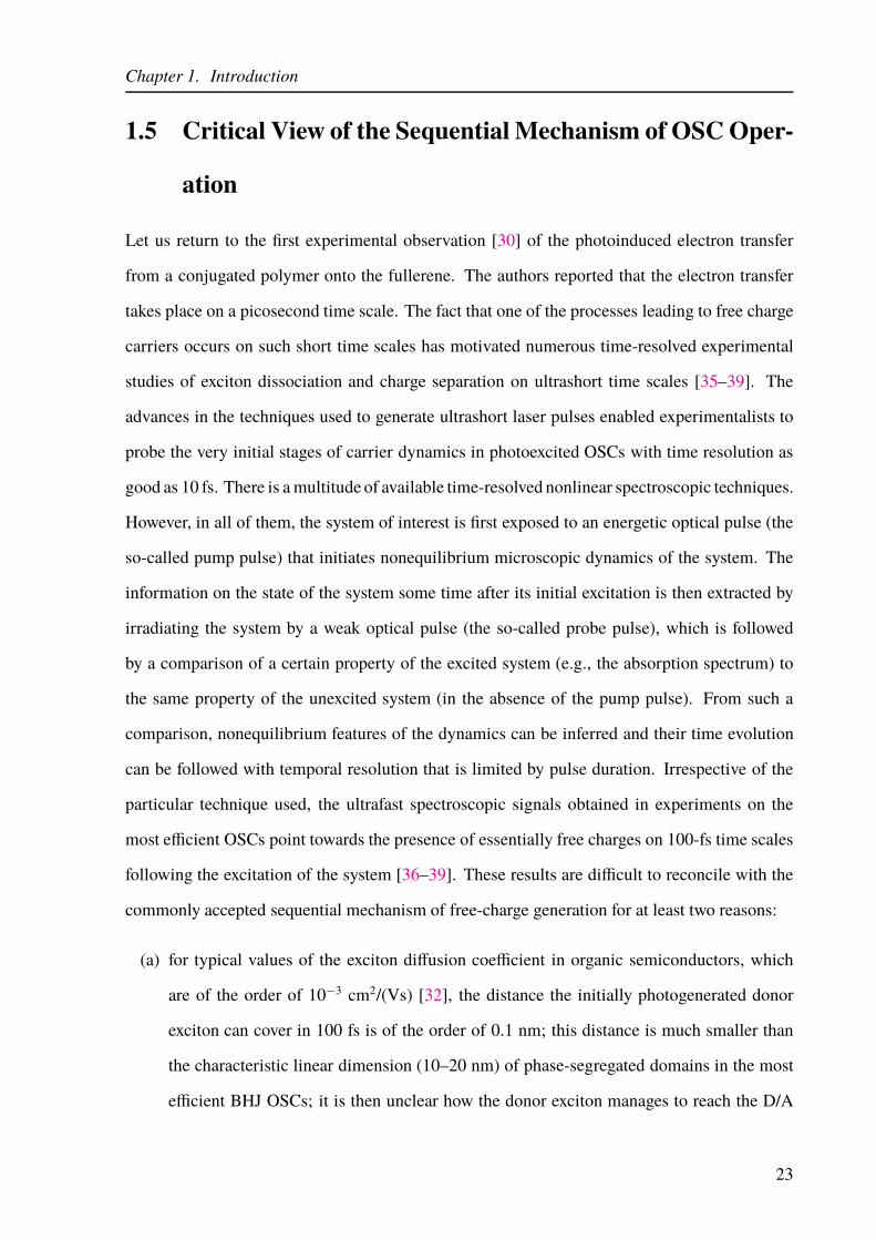
Chapter 1. Introduction
1.5 Critical View of the Sequential Mechanism of OSC Oper-
ation
Let us return to the first experimental observation [30] of the photoinduced electron transfer
from a conjugated polymer onto the fullerene. The authors reported that the electron transfer
takes place on a picosecond time scale. The fact that one of the processes leading to free charge
carriers occurs on such short time scales has motivated numerous time-resolved experimental
studies of exciton dissociation and charge separation on ultrashort time scales [35–39]. The
advances in the techniques used to generate ultrashort laser pulses enabled experimentalists to
probe the very initial stages of carrier dynamics in photoexcited OSCs with time resolution as
good as 10 fs. There is a multitude of available time-resolved nonlinear spectroscopic techniques.
However, in all of them, the system of interest is first exposed to an energetic optical pulse (the
so-called pump pulse) that initiates nonequilibrium microscopic dynamics of the system. The
information on the state of the system some time after its initial excitation is then extracted by
irradiating the system by a weak optical pulse (the so-called probe pulse), which is followed
by a comparison of a certain property of the excited system (e.g., the absorption spectrum) to
the same property of the unexcited system (in the absence of the pump pulse). From such a
comparison, nonequilibrium features of the dynamics can be inferred and their time evolution
can be followed with temporal resolution that is limited by pulse duration. Irrespective of the
particular technique used, the ultrafast spectroscopic signals obtained in experiments on the
most efficient OSCs point towards the presence of essentially free charges on 100-fs time scales
following the excitation of the system [36–39]. These results are difficult to reconcile with the
commonly accepted sequential mechanism of free-charge generation for at least two reasons:
(a) for typical values of the exciton diffusion coefficient in organic semiconductors, which
are of the order of 10−3 cm2/(Vs) [32], the distance the initially photogenerated donor
exciton can cover in 100 fs is of the order of 0.1 nm; this distance is much smaller than
the characteristic linear dimension (10–20 nm) of phase-segregated domains in the most
efficient BHJ OSCs; it is then unclear how the donor exciton manages to reach the D/A
23

Chapter 1. Introduction
interface and perform all the subsequent steps in the sequential mechanism in such a short
amount of time;
(b) even if the exciton dissociation occurs, it is not obvious what drives the transition from
the CT state towards the CS state and eventually the free-charge state on such short time
scales; this is especially controversial having in mind our estimate [Eq. (1.3)] of the bind-
ing energy of the CT exciton, which is also a measure of the energy barrier that the electron
and hole have to overcome in order to become free.
The actual mechanism of ultrafast free-charge generation in OSCs is under intense debate that
has recently inspired a great number of studies concerning exciton dissociation and charge sep-
aration that occur on ultrashort time scales, see the review articles [40–42]. The consensus on
what drives such a fast generation of free carriers, as well as on the relevance of the ultrafast
processes for the actual functioning of OSCs as electronic devices, has not been reached yet [14,
43]. In the following, we mention some of the hypotheses that have been used to explain how
OSCs perform an efficient conversion of photons to free charges despite apparently unfavorable
material characteristics.
One hypothesis is motivated by the long-lasting debate on the nature of primary photoex-
citations in conjugated polymers that reached its culmination during the last decade of the 20th
century. As discussed in more detail in Ch. 4, there are two conflicting standpoints. On the
one hand, Heeger and coworkers suggest that a photoexcitation across the band gap of a con-
jugated polymer produces the so-called free polarons, i.e., mobile charge carriers that do not
exhibit strong mutual Coulomb attraction (they are free from one another), but each of them is
accompanied by the deformation of the chain configuration [44]. On the other hand, Bässler
and coworkers highlight experimental evidence supporting the notion that strongly bound, lo-
calized, and electrically neutral excitons residing on conjugated segments that are determined by
disorder [45] are the primary photoexcitations. Actual primary photoexcitations in conjugated
polymers are in between these two limits, and their nature strongly depends on the time scale
on which they are observed. Therefore, describing the excited state of conjugated polymers as a
single species without invoking its time evolution may present a huge oversimplification of the
24
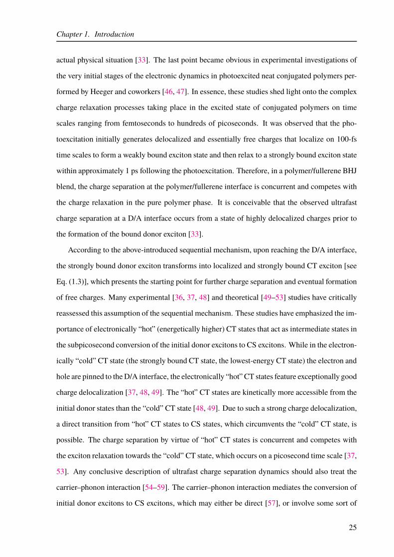
Chapter 1. Introduction
actual physical situation [33]. The last point became obvious in experimental investigations of
the very initial stages of the electronic dynamics in photoexcited neat conjugated polymers per-
formed by Heeger and coworkers [46, 47]. In essence, these studies shed light onto the complex
charge relaxation processes taking place in the excited state of conjugated polymers on time
scales ranging from femtoseconds to hundreds of picoseconds. It was observed that the pho-
toexcitation initially generates delocalized and essentially free charges that localize on 100-fs
time scales to form a weakly bound exciton state and then relax to a strongly bound exciton state
within approximately 1 ps following the photoexcitation. Therefore, in a polymer/fullerene BHJ
blend, the charge separation at the polymer/fullerene interface is concurrent and competes with
the charge relaxation in the pure polymer phase. It is conceivable that the observed ultrafast
charge separation at a D/A interface occurs from a state of highly delocalized charges prior to
the formation of the bound donor exciton [33].
According to the above-introduced sequential mechanism, upon reaching the D/A interface,
the strongly bound donor exciton transforms into localized and strongly bound CT exciton [see
Eq. (1.3)], which presents the starting point for further charge separation and eventual formation
of free charges. Many experimental [36, 37, 48] and theoretical [49–53] studies have critically
reassessed this assumption of the sequential mechanism. These studies have emphasized the im-
portance of electronically “hot” (energetically higher) CT states that act as intermediate states in
the subpicosecond conversion of the initial donor excitons to CS excitons. While in the electron-
ically “cold” CT state (the strongly bound CT state, the lowest-energy CT state) the electron and
hole are pinned to the D/A interface, the electronically “hot” CT states feature exceptionally good
charge delocalization [37, 48, 49]. The “hot” CT states are kinetically more accessible from the
initial donor states than the “cold” CT state [48, 49]. Due to such a strong charge delocalization,
a direct transition from “hot” CT states to CS states, which circumvents the “cold” CT state, is
possible. The charge separation by virtue of “hot” CT states is concurrent and competes with
the exciton relaxation towards the “cold” CT state, which occurs on a picosecond time scale [37,
53]. Any conclusive description of ultrafast charge separation dynamics should also treat the
carrier–phonon interaction [54–59]. The carrier–phonon interaction mediates the conversion of
initial donor excitons to CS excitons, which may either be direct [57], or involve some sort of
25
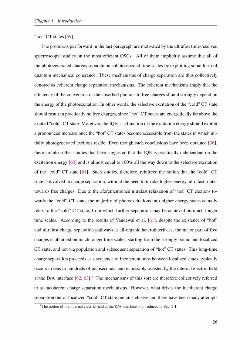
Chapter 1. Introduction
“hot” CT states [59].
The proposals put forward in the last paragraph are motivated by the ultrafast time-resolved
spectroscopic studies on the most efficient OSCs. All of them implicitly assume that all of
the photogenerated charges separate on subpicosecond time scales by exploiting some form of
quantum mechanical coherence. These mechanisms of charge separation are thus collectively
denoted as coherent charge separation mechanisms. The coherent mechanisms imply that the
efficiency of the conversion of the absorbed photons to free charges should strongly depend on
the energy of the photoexcitation. In other words, the selective excitation of the “cold” CT state
should result in practically no free charges, since “hot” CT states are energetically far above the
excited “cold” CT state. Moreover, the IQE as a function of the excitation energy should exhibit
a pronounced increase once the “hot” CT states become accessible from the states in which ini-
tially photogenerated excitons reside. Even though such conclusions have been obtained [36],
there are also other studies that have suggested that the IQE is practically independent on the
excitation energy [60] and is almost equal to 100% all the way down to the selective excitation
of the “cold” CT state [61]. Such studies, therefore, reinforce the notion that the “cold” CT
state is involved in charge separation, without the need to invoke higher-energy, ultrafast routes
towards free charges. Due to the aforementioned ultrafast relaxation of “hot” CT excitons to-
wards the “cold” CT state, the majority of photoexcitations into higher energy states actually
relax to the “cold” CT state, from which further separation may be achieved on much longer
time scales. According to the results of Vandewal et al. [61], despite the existence of “hot”
and ultrafast charge separation pathways at all-organic heterointerfaces, the major part of free
charges is obtained on much longer time scales, starting from the strongly bound and localized
CT state, and not via population and subsequent separation of “hot” CT states. This long-time
charge separation proceeds as a sequence of incoherent hops between localized states, typically
occurs in tens to hundreds of picoseconds, and is possibly assisted by the internal electric field
at the D/A interface [62, 63].1 The mechanisms of this sort are therefore collectively referred
to as incoherent charge separation mechanisms. However, what drives the incoherent charge
separation out of localized “cold” CT state remains elusive and there have been many attempts
1The notion of the internal electric field at the D/A interface is introduced in Sec. 7.1.
26
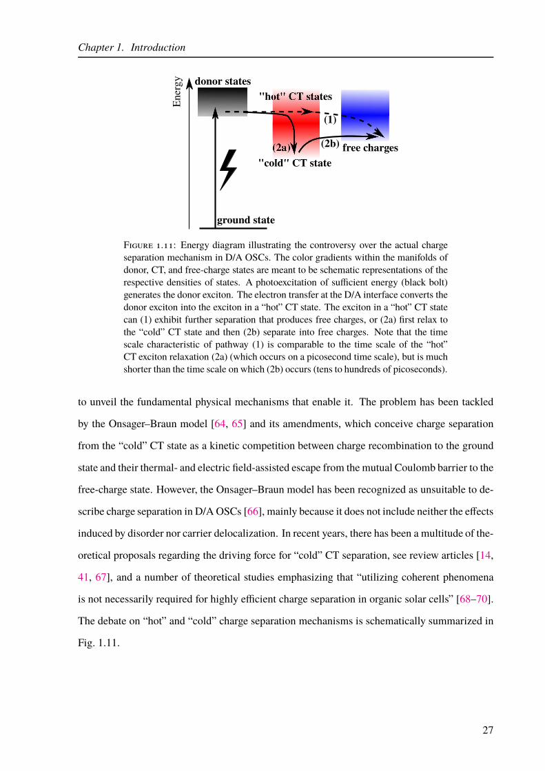
Chapter 1. Introduction
"cold" CT state
free charges
donor states
(1)
(2b)
ground state
Ener
gy
"ho tes
Figure 1.11: Energy diagram illustrating the controversy over the actual chargeseparation mechanism in D/A OSCs. The color gradients within the manifolds ofdonor, CT, and free-charge states are meant to be schematic representations of therespective densities of states. A photoexcitation of sufficient energy (black bolt)generates the donor exciton. The electron transfer at the D/A interface converts thedonor exciton into the exciton in a “hot” CT state. The exciton in a “hot” CT statecan (1) exhibit further separation that produces free charges, or (2a) first relax tothe “cold” CT state and then (2b) separate into free charges. Note that the timescale characteristic of pathway (1) is comparable to the time scale of the “hot”CT exciton relaxation (2a) (which occurs on a picosecond time scale), but is muchshorter than the time scale on which (2b) occurs (tens to hundreds of picoseconds).
to unveil the fundamental physical mechanisms that enable it. The problem has been tackled
by the Onsager–Braun model [64, 65] and its amendments, which conceive charge separation
from the “cold” CT state as a kinetic competition between charge recombination to the ground
state and their thermal- and electric field-assisted escape from the mutual Coulomb barrier to the
free-charge state. However, the Onsager–Braun model has been recognized as unsuitable to de-
scribe charge separation in D/A OSCs [66], mainly because it does not include neither the effects
induced by disorder nor carrier delocalization. In recent years, there has been a multitude of the-
oretical proposals regarding the driving force for “cold” CT separation, see review articles [14,
41, 67], and a number of theoretical studies emphasizing that “utilizing coherent phenomena
is not necessarily required for highly efficient charge separation in organic solar cells” [68–70].
The debate on “hot” and “cold” charge separation mechanisms is schematically summarized in
Fig. 1.11.
27

Chapter 1. Introduction
1.6 Organization of the Thesis
The discussion conducted in Sec. 1.5 clearly demonstrates the need for a more solid understand-
ing of fundamental physical effects that govern the light-to-charge conversion in OSCs, both on
ultrafast and on much longer time scales. To this end, the focus of this thesis will not be on one
particular material system, but rather on a detailed examination of relatively simple, yet physi-
cally plausible, model systems that capture all the physical effects that are regarded as relevant
for the phenomena of interest.
Chapter 2 introduces the so-called standard semiconductor Hamiltonian, which will be used
as a basic theoretical model throughout the thesis. We provide a formal definition of an exciton
and introduce the so-called exciton basis, which consists of the eigenstates of an electron–hole
pair that are supported by the model system. The adopted framework for description of excitons
is quite general and comprises as limiting cases the widely known Wannier and Frenkel exciton
models, which is explicitly demonstrated.
The basic theoretical tool used to investigate the ultrafast exciton dynamics within the stan-
dard semiconductor model is presented in Ch. 3. The infinite hierarchy of dynamical equations
within the density matrix formalism is truncated by means of the so-called dynamics controlled
truncation (DCT) scheme. Such a treatment is particularly suitable to describe the dynamics of
electronic excitations generated by applying an optical pulse to an initially unexcited semicon-
ductor, whose state is the vacuum of electron–hole pairs. In such a setup, many-body correlations
are ultimately induced by the applied optical field and may, therefore, be systematically classi-
fied according to the powers with which they scale in the applied field. Such a classification
enables one to perform a systematic truncation of the carrier branch of the hierarchy of equa-
tions of motion for density matrices. Previous theoretical developments in the field of inorganic
semiconductors established that a conclusive description of exciton dynamics in photoexcited
semiconductors is achieved already in the second order in the applied field. We, thus, truncate
the carrier branch of the hierarchy at the second order in the applied field, and describe our
method of the truncation of the phonon branch of the hierarchy. Our approach to the truncation
28
Chapter 1. Introduction
of the phonon branch of the hierarchy consists in proposing the form of coupling among single-
phonon-assisted and higher-order phonon-assisted density matrices that is compatible with the
energy and particle-number conservation after a pulsed optical excitation of an initially unex-
cited semiconductor. The proposed treatment of the ultrafast exciton dynamics is fully quantum
and statistical.
The essence of the proposal put forward by the Heeger’s group is that subpicosecond charge
separation at a photoexcited D/A interface is possible because it happens before the formation of
bound excitons in the donor material. This proposal calls for a theoretical investigation of the ex-
citon formation and relaxation dynamics taking place on femtosecond to picosecond time scales
in a (neat) photoexcited semiconductor. Chapter 4 of this thesis is devoted to such an investiga-
tion, which is performed on a one-dimensional two-band lattice model of a semiconductor. The
main aim of the study is the extraction of time scales relevant for the formation of the bound
excitons and their subsequent relaxation and the comparison of the time scales thus obtained
with relevant experimental data. The generality of our model enables us to study the photoin-
duced exciton dynamics for two sets of the values of model parameters, namely for the values
typical of organic and inorganic semiconductors. The exciton basis states are divided into bound
and unbound exciton states, the latter being counterparts of free-carrier states within our model.
The time scales characteristic of the exciton formation and relaxation following the excitation
of a neat semiconductor are obtained by following the time evolution of the numbers of bound
excitons and free charges. The time scales thus obtained are compared to those emerging from
subpicosecond time-resolved experiments. Furthermore, we vary different model parameters
and identify the influence of different physical effects on the time scales of interest.
In Ch. 5, we move our focus to the ultrafast exciton dynamics at photoexcited D/A interfaces,
striving to unveil the origin of spatially separated charges that have been experimentally observed
on . 100-fs time scales after the photoexcitation of the most efficient OSCs. We adjust the
theoretical model presented in Ch. 2 to the case of interest and construct a one-dimensional
lattice model of a D/A heterojunction. The theoretical method developed in Ch. 3 enables us
to treat exciton photogeneration, exciton dissociation, and further charge separation equally and
on a fully quantum level. The exciton basis states at a model D/A heterointerface are classified
29

Chapter 1. Introduction
as donor, acceptor, and space-separated states. The space-separated states are further divided
into CT and CS states according to the value of the mean electron–hole distance. Tracking the
time evolution of the numbers of excitons in donor, acceptor, CT, and CS states provides us
with a quantitative insight into the efficiency of ultrafast exciton dissociation and further charge
separation, as well as into the underlying time scales. While the conventional interpretation of
experimental results ascribes the presence of space-separated charges on ultrafast time scales
to the ultrafast population transfer from donor to space-separated states, our results suggest that
the major part of space-separated charges present on ultrafast time scales is directly optically
generated from the ground state. The direct accessibility of space-separated states from the
ground state is possible due to the resonant mixing between single-electron states in the donor
and acceptor moieties, which leads to the redistribution of oscillator strengths between donor
and space-separated states. The robustness of the principal conclusion is checked by varying
different model parameters. We also theoretically investigate ultrafast transient absorption (TA)
experiments, whose results are commonly interpreted in terms of populations only. We derive
an analytical formula for the differential transmission signal (DTS) that demonstrates that, apart
from populations, coherences should also be taken into account on such short time scales. We
find that the signal on subpicosecond time scales is actually dominated by coherences rather than
by state populations. Our findings, therefore, challenge the usual interpretation of experimental
signals on subpicosecond time scales.
The aforementioned resonant mixing, which brings about the possibility of directly reach-
ing space-separated states from the ground state, is studied in greater detail in Ch. 6, in which
we focus upon individuating the photophysical pathways that photogenerated excitations follow
on subpicosecond time scales after the photoexcitation. We find that, depending on the energy
region of the exciton spectrum, there are two ways in which the resonant mixing mechanism
can occur. The resonant mixing among single-particle states in the two materials leads to the
formation of the so-called photon-absorbing charge-bridging states, which enhance the number
of space-separated charges on ultrafast time scales by their direct optical generation, as in Ch. 5.
On the other hand, the resonant mixing among two-particle (exciton) states of donor and space-
separated character is responsible for the formation of the so-called bridge states that enhance
30

Chapter 1. Introduction
the ultrafast generation of separated charges by acting as intermediate states in phonon-assisted
transitions from donor states towards space-separated states. We conclude that, on subpicosec-
ond time scales, free-charge generation is governed by the competition between transitions from
the donor to the space-separated manifold and transitions within the donor manifold. While
the former type of transitions may enhance free-charge generation, the latter type of transitions
leads to the relaxation towards the lowest-energy donor state, which acts as a trap for charge
separation. Our numerical results demonstrate that, at ∼ 1 ps following the excitation, the major
part of photogenerated excitons remains in the donor exciton manifold. Moreover, on the same
time scales, we also observe some relaxation within the space-separated manifold towards the
strongly bound CT state.
While indicating that there is some build-up of the populations of space-separated states on
ultrafast time scales, the results obtained in Ch. 6 strongly suggest that, if the charge separation
at a D/A interface is effective, it is expected to predominantly occur on time scales that are much
longer than the picosecond one, from the strongly bound and localized donor or CT states. As
we have already discussed, such a scenario is typical of incoherent (“cold”) separation mecha-
nisms, which, however, do not provide us with the driving force enabling charge separation from
localized initial conditions. Our efforts summarized in Ch. 7 are aimed at identifying the phys-
ical effects that are responsible for the experimentally observed efficient and electric field- and
temperature-independent separation of strongly bound charge pairs. The model is essentially the
same as in Chapter 6, but in Ch. 7 it also takes into account the presence of the disorder, which
is ubiquitous in organic semiconductors. Differently from many proposed models of incoherent
charge separation, our model fully and properly takes into account charge delocalization effects,
whose relevance has been repeatedly recognized. We find that the combination of charge delo-
calization and disorder is at the heart of efficient and weakly field- and temperature-dependent
charge separation from both the strongly bound CT and donor exciton states.
Chapter 8 is devoted to a summary of the most important conclusions emerging from the
investigations presented in this thesis.
31

Chapter 2
Standard Semiconductor Model
Here, we introduce the standard semiconductor model, which is the basic theoretical model
that will be used throughout this thesis. Since this model should provide us with insights into
microscopic processes taking place in photoexcited semiconductors on ultrafast time scales, it
has to account for relevant physical effects such as
(a) the charge delocalization, which leads to the formation of bands,
(b) the electron–hole interaction, which is responsible for exciton formation,
(c) the carrier–phonon interaction, which determines the relaxation properties of the system,
and
(d) the interaction of carriers with the external electromagnetic field that creates interband
(electron–hole) excitations.
In Sec. 2.1, we introduce the two-band semiconductor model, consisting of one conduction band
and one valence band. The generalization to the multiband case is straightforward and will be
used in certain parts of the thesis. The standard semiconductor model is thoroughly presented
from various viewpoints in a number of review articles [71–73] and books [74, 75]. Here, we
follow the analysis presented in Ref. [71]. Section 2.2 defines an exciton as the simplest excitation
above the ground state of a semiconductor. While the developments in Secs. 2.1 and 2.2 are quite
general, in Sec. 2.3 we are more specific and demonstrate that, under appropriate approximations,
the model we use can reduce to the widely known Wannier and Frenkel exciton models.
32

Chapter 2. Standard Semiconductor Model
2.1 Two-Band Semiconductor Model
The Hamiltonian of a system of nonrelativistic valence electrons interacting with lattice vibra-
tions (phonons) and with an external optical field can be expressed as
H = Hmat +Hp +Hmat−p +Hmat−f . (2.1)
The first and the second term describe isolated carriers and phonons, the third term is the carrier–
phonon interaction, while the fourth term represents the interaction of carriers with the external
electromagnetic field. For the sake of simplicity, unless otherwise stated, we will not explicitly
consider the electron spin, but assume that the spin quantum number is absorbed into the generic
quantum number for electronic excitations. Using the second-quantized field operatorsΨ(r) and
Ψ†(r), the part of the Hamiltonian that describes isolated carriers reads as
Hmat =
∫
drΨ†(r)H0(r)Ψ(r) +1
2
∫
dr1 dr2 Ψ†(r1)Ψ
†(r2)Vc−c(r1 − r2)Ψ(r2)Ψ(r1). (2.2)
H0(r) is the single-electron Hamiltonian, which comprises the kinetic energy of an electron and
the single-particle potential created by the nuclei and core electrons. Vc−c(r1 − r2) denotes the
Coulomb interaction potential screened by the core electrons and lattice degrees of freedom that
are not accounted for dynamically. The Fermi field operators Ψ(r) [Ψ†(r)] annihilate [create]
an electron in r and satisfy the anticommutation relations
Ψ(r),Ψ(r′) = 0,Ψ(r),Ψ†(r′)
= δ(r− r′). (2.3)
The free-phonon part of the Hamiltonian is
Hp =∑
µ
~ωµb†µbµ, (2.4)
33

Chapter 2. Standard Semiconductor Model
where bµ (b†µ) are Bose operators destroying (creating) a phonon in mode µwith energy ~ωµ and
obeying the commutation relations
[bµ, bν ] = 0,[bµ, b
†ν
]= δµν . (2.5)
The coupling between carriers and lattice vibrations is described by
Hmat−p =
∫
drΨ†(r)Vc−p(r)Ψ(r), (2.6)
where
Vc−p(r) =∑
µ
(gµ(r)b
†µ + g∗µ(r)bµ
)(2.7)
is the potential induced by the lattice vibrations, in which only terms linear in the displacements
of the nuclei have been retained. Finally, the interaction with the optical field E(t) is of the form
Hmat−f = −E(t)
∫
drΨ†(r) (−er) Ψ(r). (2.8)
Since our main aim is to study time-dependent phenomena in semiconductors (and their het-
erojunctions) excited by a laser pulse, we assume that the electric field is spatially homoge-
neous. The spatial dependence of the field can be included in a straightforward manner, see,
e.g., Ref. [72].
Let us study in more detail the ground state of the interacting-carrier Hamiltonian [Eq. (2.2)].
The simplest possible approximation to the true ground state of a system of interacting fermions
is the Hartree–Fock ground state, which is a single Slater determinant consisting of occupied
single-particle states that are determined by the variational approach. Namely, by requiring that
the ground-state energy be minimal, we obtain the set of Hartree–Fock equations, the solution
to which provides us with the aforementioned single-particle states. We introduce new Fermi
operators ap, a†p by
Ψ(r) =∑
p
φp(r)ap, (2.9)
34

Chapter 2. Standard Semiconductor Model
where φp(r) are orthonormal single-particle wave functions labeled by index p. Operators ap, a†p
obey the following anticommutation laws
ap, ap′ = 0,
ap, a†p′
= δpp′, (2.10)
and will be further referred to as particle operators, while computations performed using particle
operators are said to be performed in the particle picture. The ground state of Hmat is then
approximated as
|GS〉 =∏
p∈occ
a†p|0〉e, (2.11)
where |0〉e is the particle vacuum, and “occ” denotes the set of occupied single-particle states.
The wave functions φp(r) are determined by requiring that the energy of the ground state |GS〉,
〈GS|Hmat|GS〉 =∑
p∈occ
tpp +1
2
∑
pq∈occ
(Vppqq − Vpqqp) , (2.12)
be minimal. In other words, these wave functions satisfy the Hartree–Fock equations
H0(r)φp(r) +∑
p′∈occ
∫
dr′φ∗p′(r
′)Vc−c(r− r′) [φp′(r′)φp(r)− φp(r
′)φp′(r)] = ǫp φp(r), (2.13)
where ǫp are the energies of Hartree–Fock orbitals. In Eq. (2.12), we introduce matrix elements
tpq of the single-particle Hamiltonian H0
tpq =
∫
dr φ∗p(r)H0(r)φq(r), (2.14)
as well as matrix elements Vpqkl of the Coulomb interaction
Vpqkl =
∫
dr1 dr2 φ∗p(r1)φq(r1)Vc−c(r1 − r2)φ
∗k(r2)φl(r2). (2.15)
35

Chapter 2. Standard Semiconductor Model
The energy difference between the lowest unoccupied and the highest occupied single-particle
states (in the ground state of the carrier subsystem)
Eg = minp/∈occ
ǫp −maxp∈occ
ǫp (2.16)
in a typical semiconductor isEg ∼ 1 eV and is denoted as the single-particle band gap. SinceEg
is much larger than the thermal energy at room temperature, we may safely assume that, in the
absence of an optical excitation of sufficient energy, the carrier subsystem is in the Hartree–Fock
ground state [Eq. (2.11)].
The preceding developments make it easy to differentiate between occupied and unoccu-
pied states with respect to the Hartree–Fock ground state. In other words, we may transfer the
description of a semiconductor from the particle picture to the so-called electron–hole picture.
The particles in initially unoccupied states are further referred to as electrons. The absence of
a particle in an initially occupied state is further denoted as a hole. We define creation (d†p) and
annihilation (dp) operators for holes as
d†p = ap, dp = a†p, for p ∈ occ. (2.17)
The definitions of electron creation (c†p) and annihilation (cp) operators are
c†p = a†p, cp = ap, for p /∈ occ. (2.18)
In a semiconductor, the band gap separates the valence band, which is fully occupied, from the
conduction band, which is completely empty. We assume that the spectrum of both occupied
and unoccupied single-particle states is dense, i.e., occupied states form a single band of states
that is further denoted as the valence band, while unoccupied states also form a single band
further referred to as the conduction band. In further analysis, single-particle states p ∈ occ that
are occupied in the ground state |GS〉 will be considered as valence-band states and denoted as
p ∈ VB, while single-particle states p /∈ occ that are empty in the ground state |GS〉 will be
considered as conduction-band states and denoted as p ∈ CB. The electron and hole operators
36
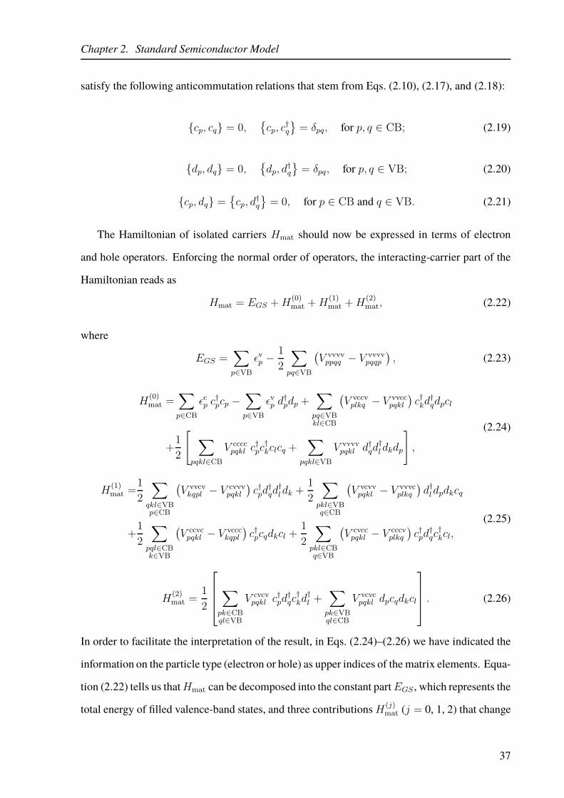
Chapter 2. Standard Semiconductor Model
satisfy the following anticommutation relations that stem from Eqs. (2.10), (2.17), and (2.18):
cp, cq = 0,cp, c
†q
= δpq, for p, q ∈ CB; (2.19)
dp, dq = 0,dp, d
†q
= δpq, for p, q ∈ VB; (2.20)
cp, dq =cp, d
†q
= 0, for p ∈ CB and q ∈ VB. (2.21)
The Hamiltonian of isolated carriers Hmat should now be expressed in terms of electron
and hole operators. Enforcing the normal order of operators, the interacting-carrier part of the
Hamiltonian reads as
Hmat = EGS +H(0)mat +H
(1)mat +H
(2)mat, (2.22)
where
EGS =∑
p∈VB
ǫvp −1
2
∑
pq∈VB
(V vvvvppqq − V vvvv
pqqp
), (2.23)
H(0)mat =
∑
p∈CB
ǫcp c†pcp −
∑
p∈VB
ǫvp d†pdp +
∑
pq∈VBkl∈CB
(V vccvplkq − V vvcc
pqkl
)c†kd
†qdpcl
+1
2
[∑
pqkl∈CB
V ccccpqkl c
†pc
†kclcq +
∑
pqkl∈VB
V vvvvpqkl d†qd
†ldkdp
]
,
(2.24)
H(1)mat =
1
2
∑
qkl∈VBp∈CB
(V vvcvkqpl − V cvvv
pqkl
)c†pd
†qd
†ldk +
1
2
∑
pkl∈VBq∈CB
(V vcvvpqkl − V vvvc
plkq
)d†ldpdkcq
+1
2
∑
pql∈CBk∈VB
(V ccvcpqkl − V vccc
kqpl
)c†pcqdkcl +
1
2
∑
pkl∈CBq∈VB
(V cvccpqkl − V cccv
plkq
)c†pd
†qc
†kcl,
(2.25)
H(2)mat =
1
2
∑
pk∈CBql∈VB
V cvcvpqkl c
†pd
†qc
†kd
†l +
∑
pk∈VBql∈CB
V vcvcpqkl dpcqdkcl
. (2.26)
In order to facilitate the interpretation of the result, in Eqs. (2.24)–(2.26) we have indicated the
information on the particle type (electron or hole) as upper indices of the matrix elements. Equa-
tion (2.22) tells us thatHmat can be decomposed into the constant partEGS , which represents the
total energy of filled valence-band states, and three contributionsH(j)mat (j = 0, 1, 2) that change
37

Chapter 2. Standard Semiconductor Model
the number of electron–hole pairs by j pairs. Apart from the constant part, which amounts to a
shift of the energy axis, in this thesis we will also disregard all the contributions that do not con-
serve the number of electron–hole pairs and focus our attention on the pair-conserving partH(0)mat.
The approximation that neglects contributions that do not preserve the number of electron–hole
pairs will be viewed from somewhat different perspective in Sec. 2.3.2 devoted to the Frenkel
exciton model.
The Coulomb matrix elements appearing in Eq. (2.24) can be divided into direct and ex-
change terms. If the arguments in the Coulomb matrix element can be grouped to give electron
or hole densities of the respective single-particle states, as is the case in terms V vvccpqkl , V cccc
pqkl , and
V vvvvpqkl , this matrix element represents a direct term. On the other hand, Coulomb matrix element
V vccvplkq is an example of an exchange term.
The carrier–phonon interaction is expressed in terms of electron and hole operators as
Hmat−p = H(0)mat−p +H
(1)mat−p +H
(f)mat−p, (2.27)
where
H(0)mat−p =
∑
pq∈CB
∑
µ
(γµpq c
†pcqb
†µ + γµ∗pq c
†qcpbµ
)+∑
pq∈VB
∑
µ
(γµpqd
†qdpb
†µ + γµ∗pq d
†pdqbµ
), (2.28)
H(1)mat−p =
∑
p∈VBq∈CB
∑
µ
(γµpqdpcqb
†µ + γµ∗pq c
†qd
†pbµ)+∑
p∈CBq∈VB
∑
µ
(γµpqc
†pd
†qb
†µ + γµ∗pq dqcpbµ
), (2.29)
H(f)mat−p =
∑
pq∈VB
δpq(γµpqb
†µ + γµ∗pq bµ
). (2.30)
The carrier–phonon matrix element between two single-particle states reads as
γµpq =
∫
dr φ∗p(r) g(r) φq(r). (2.31)
The decomposition of the carrier–phonon interaction Hamiltonian embodied in Eq. (2.27) is
similar to the decomposition of the purely carrier Hamiltonian in Eq. (2.22). The contribu-
tionH(f)mat−p represents the carrier–phonon interaction energy in the Hartree–Fock ground state.
38

Chapter 2. Standard Semiconductor Model
Since its action is limited to phonon degrees of freedom, this term does not contribute to the hole–
phonon coupling and will not be considered in further discussion. The contributions H(j)mat−p
(j = 0, 1) change the number of electron–hole pairs by j pairs. H(1)mat−p describes phonon-
induced transitions among occupied and unoccupied states. Having in mind that the energy gap
separating these two groups of states is of the order of 1 eV, such transitions are not very probable
in common semiconductor materials. Therefore, we further consider only contributionH(0)mat−p,
which conserves the number of electron–hole pairs.
The interaction with the optical field can be recast in terms of electron and hole operators as
Hmat−f =− E(t)
∑
p∈VBq∈CB
Mvcpqdpcq +
∑
p∈CBq∈VB
Mcvpqc
†pd
†q
− E(t)
(∑
pq∈CB
Mccpqc
†pcq +
∑
pq∈VB
Mvvpqd
†qdp
)
,
(2.32)
where the dipole-moment matrix elements are defined as
Mpq =
∫
dr φ∗p(r) (−er)φq(r). (2.33)
The first term in Eq. (2.32) describes the so-called interband transitions, in which the optical field
of sufficient frequency promotes an electron from the valence band to the conduction band and
creates an electron–hole pair. On the other hand, the second term in Eq. (2.32) describes the so-
called intraband transitions that take place within the conduction or valence band. In this thesis,
the focus is on the detailed understanding of processes occurring during and after the excitation
of a neat semiconductor (or a heterojunction of two semiconductors) that creates electron–hole
pair excitations. Therefore, in the major part of the thesis, the second term in Eq. (2.32) will not
be considered. An exception will be made in our theoretical treatment of a transient absorption
experiment in Sec. 5.4.2.
In summary, we explicitly write down the model Hamiltonian that will be used throughout
this thesis
H = Hc +Hp +Hc−p +Hc−f , (2.34)
39

Chapter 2. Standard Semiconductor Model
Hc =∑
p∈CB
ǫcp c†pcp −
∑
p∈VB
ǫvp d†pdp +
∑
pq∈VBkl∈CB
(V vccvplkq − V vvcc
pqkl
)c†kd
†qdpcl
+1
2
[∑
pqkl∈CB
V ccccpqkl c
†pc
†kclcq +
∑
pqkl∈VB
V vvvvpqkl d†qd
†ldkdp
]
,
(2.35)
Hp =∑
µ
~ωµb†µbµ, (2.36)
Hc−p =∑
pq∈CB
∑
µ
(γµpq c
†pcqb
†µ + γµ∗pq c
†qcpbµ
)
+∑
pq∈VB
∑
µ
(γµpqd
†qdpb
†µ + γµ∗pq d
†pdqbµ
),
(2.37)
Hc−f = −E(t)
∑
p∈VBq∈CB
Mvcpqdpcq +
∑
p∈CBq∈VB
Mcvpqc
†pd
†q
. (2.38)
The model Hamiltonian given in Eqs. (2.34)–(2.38) is known in literature as the standard semi-
conductor Hamiltonian.
The derivation of the model Hamiltonian has produced the diagonal single-particle contri-
bution in Eq. (2.35). In actual modeling, this part does not have to be diagonal, so that it may
be replaced by
∑
p∈CB
ǫcp c†pcp −
∑
p∈VB
ǫvp d†pdp →
∑
pq∈CB
ǫcpq c†pcq −
∑
pq∈VB
ǫvqp d†pdq. (2.39)
The last point will be useful in the construction of models describing charge separation at inter-
faces between two semiconductors.
All the interactions present in the model Hamiltonian embodied in Eqs. (2.34)–(2.38) are
spin-independent. Let us now explicitly separate the spin quantum number σp out of the generic
quantum number p, p = (po, σp), where po is the orbital quantum number. This step has to
be accompanied by a more specific definition of the hole creation and annihilation operators
[Eq. (2.17)]. Namely, the annihilation of an electron with spin σ in a valence-band state can
also be seen as the creation of a hole with spin σ = −σ in the same valence-band state, i.e.,
d†po,σp= apo,σp
. Moreover, if valence-band states are labeled by wave vector k, the annihilation
40

Chapter 2. Standard Semiconductor Model
of an electron in the valence-band state (k, σ) can be conceived as the creation of a hole with
wave vector −k and spin −σ,1
d†−k,−σ = ak,σ. (2.40)
Taking the last fact into account, the termsHc [Eq. (2.35)],Hc−p [Eq. (2.37)], andHc−f [Eq. (2.38)]
of the standard semiconductor Hamiltonian, in which the spin quantum number is explicitly con-
sidered, read as
Hc =∑
po∈CB
∑
σ
ǫcpo c†poσcpoσ −
∑
po∈VB
∑
σ
ǫvpo d†poσdpoσ
+∑
poqo∈VBkolo∈CB
∑
σpσk
(
V vccvpolokoqoc
†koσk
d†qoσkdpoσp
cloσp− V vvcc
poqokoloc†koσk
d†qoσpdpoσp
cloσk
)
+1
2
∑
poqokolo∈CB
∑
σpσk
V ccccpoqokolo c
†poσp
c†koσkcloσk
cqoσp
+1
2
∑
poqokolo∈VB
∑
σpσk
V vvvvpoqokolo d
†qoσp
d†loσkdkoσk
dpoσp,
(2.41)
Hc−p =∑
poqo∈CB
∑
σ
∑
µ
(γµpoqo c
†poσcqoσb
†µ + γµ∗poqoc
†qoσcpoσbµ
)
+∑
poqo∈VB
∑
σ
∑
µ
(γµpoqod
†qoσdpoσb
†µ + γµ∗poqod
†poσdqoσbµ
),
(2.42)
Hc−f = −E(t)
∑
po∈VBqo∈CB
∑
σ
Mvcpoqodpoσcqoσ +
∑
po∈CBqo∈VB
∑
σ
Mcvpoqoc
†poσd
†qoσ
. (2.43)
Let us also notice that the above-presented developments are quite general and do not rely
on specific assumptions regarding indices that label single-particle states. The model Hamilto-
nian is, therefore, flexible, as will be shown in greater detail in Secs. 2.3.1 and 2.3.2, where we
explicitly demonstrate that it can be applied to study Wannier and Frenkel excitons.
1The hole operators may be formally introduced by applying a time reversal transformation to particle operators,see, e.g., Ref. [76]. The time reversal introduces a minus sign in front of the momentum (and spin), so that the wavevector (and spin) associated with a hole acquire an additional minus sign.
41

Chapter 2. Standard Semiconductor Model
2.2 Definition of Exciton
The ground state |GS〉 of a semiconductor in the Hartree–Fock approximation [Eq. (2.11)] can
also be regarded as the vacuum of electron–hole pairs and will be further denoted as |0〉. In a
singly excited state, an electron is promoted to the conduction band, leaving behind a hole in the
valence band, i.e., there is an electron–hole pair. The excited electron and hole are coupled by
the Coulomb interaction. The most general electron–hole pair state is the superposition
|x〉 =∑
a∈VBb∈CB
ψxab c
†bd
†a|0〉, (2.44)
where the amplitudeψxab describes the contribution of the pair state in which an electron initially
in valence-band state a is promoted to conduction-band state b. The exciton basis is defined by
the eigenvalue problem
Hc|x〉 = ~ωx|x〉, (2.45)
which, due to the linear independence of different pair states c†bd†a|0〉, can be written as the fol-
lowing equation for amplitudes ψxab
(ǫcb − ǫva)ψxab +
∑
p∈VBq∈CB
(V vccvpqba − V vvcc
pabq
)ψxpq = ~ωxψ
xab. (2.46)
The amplitude ψxab may also be expressed as the scalar product ψx
ab = 〈ahbe|x〉 of two vectors
in the space of single electron–hole excitations. Since exciton states |x〉 are orthonormal, the
following identity holds∑
a∈VBb∈CB
ψx′∗ab ψ
xab = δx′x. (2.47)
Exciton states |x〉 constitute a basis in the space of single electron–hole excitations, so that
the decomposition of unity in this space gives the following relation
∑
x
ψx∗a′b′ψ
xab = δa′aδb′b. (2.48)
42

Chapter 2. Standard Semiconductor Model
The operator that creates an exciton in state |x〉 is denoted asX†x and introduced by |x〉 = X†
x|0〉.
In terms of electron and hole operators,
X†x =
∑
a∈VBb∈CB
ψxab c
†bd
†a. (2.49)
Using the anticommutation relations of electron and hole operators [Eqs. (2.19)–(2.21)], we
obtain that exciton operators Xx, X†x satisfy the following relations
[Xx, Xx′] =[
X†x, X
†x′
]
= 0, (2.50)
[
Xx, X†x′
]
= δxx′ −∑
a′a∈VB
(∑
b∈CB
ψx∗abψ
x′
a′b
)
d†a′da −∑
b′b∈CB
(∑
a∈VB
ψx∗abψ
x′
ab′
)
c†b′cb. (2.51)
When the density of electronic excitations is small, Eqs. (2.50) and (2.51) suggest that excitons
can be regarded as bosons.
Let us now complete our discussion on excitons by explicitly considering the spin quantum
number. According to their spin multiplicity, exciton states can be classified as singlet or triplet
states. The space of single electron–hole excitations, which is spanned by vectors
|(aoσa)h(boσb)e〉 = c†boσbd†aoσa
|0〉
, (2.52)
can be divided into subspaces with well-defined spin multiplicity according to the eigenvalues
of operators S2 and Sz, where the operator of the total spin S is defined as
S =∑
σ′σ
⟨
σ′
∣∣∣∣
~
2τ
∣∣∣∣σ
⟩(∑
po∈CB
c†poσ′cpoσ −∑
po∈VB
d†poσdpoσ′
)
. (2.53)
In the last equation, τ are Pauli matrices. In the subspace of singlet excitons, both S2 and Sz
reduce to zero, and the corresponding basis vectors are [77, 78]
|(ao)h(bo)e〉S =1√2
(
c†bo,↑d†ao,↓
+ c†bo,↓d†ao,↑
)
|0〉
. (2.54)
43

Chapter 2. Standard Semiconductor Model
In the subspace of triplet excitons, operator S2 reduces to 2, while, according to the eigenvalue
of Sz, we have the following groups of basis vectors
|(ao)h(bo)e〉T,0 =1√2
(
c†bo,↑d†ao,↓
− c†bo,↓d†ao,↑
)
|0〉
, (2.55a)
|(ao)h(bo)e〉T,1 = c†bo,↑d†ao,↑
|0〉
, (2.55b)
|(ao)h(bo)e〉T,−1 = c†bo,↓d†ao,↓
|0〉
. (2.55c)
Therefore, the most general singlet exciton state is of the form
|x〉S =∑
ao∈VBbo∈CB
ψx,Saobo
|(ao)h(bo)e〉S , (2.56)
where the expansion coefficients ψx,Saobo
satisfy an equation analogous to Eq. (2.46) that reads as
(ǫcbo − ǫvao
)ψx,Saobo
+∑
po∈VBqo∈CB
(2V vccv
poqoboao − V vvccpoaoboqo
)ψx,Spoqo = ~ωx,Sψ
x,Saobo
. (2.57)
Similarly, the most general triplet exciton state with a fixed value of Sz is
|x〉T,Sz=∑
ao∈VBbo∈CB
ψx,(T,Sz)aobo
|(ao)h(bo)e〉T,Sz, (2.58)
and the expansion coefficients satisfy
(ǫcbo − ǫvao
)ψ
x,(T,Sz)aobo
−∑
po∈VBqo∈CB
V vvccpoaoboqoψ
x,(T,Sz)poqo = ~ωx,(T,Sz)ψ
x,(T,Sz)aobo
. (2.59)
Let us mention that Eqs. (2.57) and (2.59) are usually written as a single equation for the expan-
sion coefficients ψxaobo
in the orbital space
(ǫcbo − ǫvao
)ψxaobo +
∑
po∈VBqo∈CB
(2δMV
vccvpoqoboao − V vvcc
poaoboqo
)ψxpoqo = ~ωxψ
xaobo , (2.60)
44

Chapter 2. Standard Semiconductor Model
where δM = 1 for singlet excitons and δM = 0 for triplet excitons. A photoexcitation of a semi-
conductor whose form is given in Eq. (2.38) [or Eq. (2.43)] can generate only singlet excitons.
We usually say that singlet excitons are optically active, while triplet excitons are optically inac-
tive. Since the time evolution driven by the standard semiconductor Hamiltonian cannot change
spin multiplicity of photogenerated singlet excitons, we conclude that, in all of our theoretical
developments concerning exciton dynamics, we will have to deal exclusively with singlet ex-
citons. In reality, however, the spin–orbit coupling, i.e., the interaction between the spin and
orbital motion of an electron, brings about mixing between singlet and triplet excitations [79].
An excitation transfer from the singlet to the triplet manifold is commonly denoted as the inter-
system crossing. Our focus in the forthcoming chapters will be on exciton dynamics occurring
on femtosecond to picosecond time scales following the photoexcitation of organic semiconduc-
tors and their heterojunctions. However, the intersystem crossing in these systems typically takes
place on much longer time scales, spanning the range from nanoseconds to microseconds [79,
80]. Therefore, the intersystem crossing is not active on time scales of our interest, and confining
the investigations to the singlet subspace provides us with relevant insights into ultrafast exciton
dynamics.
We will not further dwell on the spin multiplicity of exciton states. To compute the (singlet)
exciton basis states, we will use Eq. (2.46) remembering that, according to Eq. (2.57), a factor
of 2 should be inserted in front of the exchange term.
2.3 Wannier and Frenkel Exciton Models
In this section, we discuss which approximations should be employed in order to obtain the
widely known Wannier [81] and Frenkel [82, 83] exciton models. The analysis concerning the
Wannier model is mainly based on Ch. 2 of Ref. [76] and Ch. 23 of Ref. [84], while the micro-
scopic model for Frenkel excitons is developed in Ch. 24 of Ref. [84] and also in Ref. [85]. An
excellent classical text on these two models of excitons can be found Ref. [86].
45
Chapter 2. Standard Semiconductor Model
2.3.1 Wannier Exciton Model
Let us now specialize to the case of a crystalline semiconductor consisting of Nuc periodically
repeated unit cells. The single-particle states in both the valence and the conduction band can
then be counted by wave vector k, and the corresponding wave functions are (λ ∈ v, c)
φλk(r) =
1√Nuc
uλk(r) eik·r, (2.61)
where Bloch functions uλk(r) have the periodicity of the lattice. The explicit separation of the
factor 1/√Nuc out of the wave function φλ
k(r) ensures that Bloch functions are normalized to 1
within a unit cell∫
vuc
dr∣∣uλk(r)
∣∣2= 1, (2.62)
where vuc is the volume of the unit cell. We further assume that we deal with a direct semicon-
ductor with isotropic effective masses m∗e and m∗
h for electrons and holes, respectively, so that
the single-particle energies in the vicinity of the valence-band maximum (and conduction-band
minimum) k = 0 can be expressed as
ǫck = Eg +~2k2
2m∗e
, ǫvk = −~2k2
2m∗h
, (2.63)
where Eg is the single-particle gap of the semiconductor (at k = 0), see also Eq. (2.16). The
eigenvalue problem that should be solved to obtain exciton basis states [Eq. (2.46)] can be spe-
cialized to the case of interest to give
(ǫcke
− ǫv−kh
)ψxkhke
+∑
lhle
(V vccv−lhleke−kh
− V vvcc−lh−khkele
)ψxlhle
= ~ωxψxkhke
. (2.64)
Let us analyze in more detail the direct term of the electron–hole interaction
V vvcc−lh−khkele
=1
N2uc
∫
Ω
drh dre ei(lh−kh)·rh ei(le−ke)·re Vc−c(re − rh)
× uv∗−lh(rh) u
v−kh
(rh) uc∗ke(re) u
cle(re),
(2.65)
46

Chapter 2. Standard Semiconductor Model
where the integrations are performed over the entire volume Ω of the crystal. The exchange
term can be written in a similar manner. For electronic excitations in the vicinity of the band
extrema (k = 0), the plane-wave factors, as well as the Coulomb potential, are slowly varying
functions whose changes within one unit cell are very small. These simplifying assumptions are
due to Wannier [81] and are appropriate for weakly bound pair states, in which the electron–hole
separation is large compared to the lattice constant and the wave vector of the relative motion
of the electron and hole is small compared to the inverse lattice constant. The integrations in
Eq. (2.67) can be split into the summations over all unit cells and the integrations over the volume
of a unit cell vuc. The Bloch functions are then be expanded around k = 0 and only the first,
constant in k, term is retained. Using the aforementioned assumptions together with the lattice
periodicity of the Bloch functions, we obtain the following integrals
∫
vuc
dr uc∗k≃0(r) ucl≃0(r) ≃ 1,
∫
vuc
dr uc∗k≃0(r) uvl′≃0(r) ≃ 0. (2.66)
Therefore, in this approximation, the exchange term vanishes. Since the length scales of rele-
vance are much larger than the lattice constant, in the direct term we can transfer to the continuum
representation and obtain
V vvcc−lh−khkele
=1
Ω2
∫
Ω
dre drh ei(lh−kh)·rh ei(le−ke)·re Vc−c(re − rh). (2.67)
Equation (2.67) shows us that the total wave vector of the pair,
K = ke + kh = le + lh, (2.68)
is a good quantum number, and that the direct term V vvcc−lh−khkele
is proportional to the Fourier
transformation Vc−c (|lh − kh|) of the Coulomb potential.
Having substituted the results given in Eqs. (2.63) and (2.67) into Eq. (2.64), further ma-
nipulations in Eq. (2.64) are facilitated by introducing the Fourier transformation of amplitudes
47

Chapter 2. Standard Semiconductor Model
ψxkhke
ψxrhre
=∑
khke
eikh·rh eike·re ψxkhke
. (2.69)
The Fourier transformation of Eq. (2.64) then gives
(
− ~2
2m∗e
∇2e −
~2
2m∗h
∇2h + Eg − Vc−c(re − rh)
)
ψxrhre
= ~ωxψxrhre
. (2.70)
Since Eq. (2.70) is actually a two-body problem, it is convenient to separate the motion of the
center of mass of the pair (coordinate R) and the relative motion of the electron and hole com-
posing the pair (coordinate r) by introducing
R =m∗
e
m∗e +m∗
h
re +m∗
h
m∗e +m∗
h
rh, r = re − rh. (2.71)
The motion of the center of mass can be described by a plane wave with wave vector K. The
relative motion is described by quantity ψx,relr which is defined as
ψxrhre
=1√Ω
eiK·R ψx,relr , (2.72)
and satisfies
(
− ~2
2mred
∇2 − Vc−c(r)
)
ψx,relr =
(
~ωx −Eg −~2K2
2(m∗e +m∗
h)
)
ψx,relr . (2.73)
In the last equation, mred =m∗
em∗h
m∗e+m∗
h
is the reduced mass of the pair. If we model the Coulomb
interaction potential as
Vc−c(r) =1
4πε0
e2
εr|r|, (2.74)
where εr is the relative dielectric constant of the medium, we see that Eq. (2.73) is analogous
to the equation satisfied by the stationary states of the hydrogen atom. Therefore, the solutions
to Eq. (2.73) are counted by quantum number n = 1, 2, . . . , and pair states can be uniquely
identified by specifying the wave vector of the center of mass K and n, i.e., label x can be
replaced by (K, n). In other words, there is the internal motion of an electron around a hole
48

Chapter 2. Standard Semiconductor Model
(described by the quantum number n) that is accompanied by the motion of the pair as a whole
throughout the crystal (characterized by the center-of-mass wave vector K). The total energy of
state (K, n) is given as
~ωK,n = Eg +~2K2
2(m∗e +m∗
h)+ ǫn, (2.75)
where
ǫn = − mrede4
32π2ε20ε2r
1
n2. (2.76)
The energy spectrum of an electron–hole pair contains a number of bound pair states and the
continuum of ionized (unbound) states. The binding energy of the lowest-energy exciton state
(K = 0, n = 1) is usually referred to as the exciton binding energy and is given as
ǫXb =mrede
4
32π2ε20ε2r
, (2.77)
while the corresponding Bohr radius, which is a measure of the electron–hole separation in
bound states, is
a0,X =4πε0εr~
2
mrede2. (2.78)
Compared to the hydrogen atom, the exciton binding energy is reduced because the reduced
mass of the pair is smaller than the free-electron mass and the Coulomb interaction is screened,
so that
ǫXb =mred
me
1
ε2r
mee4
32π2ε20=mred
me
1
ε2r× 13.6 eV, (2.79)
and
a0,X = εr
(mred
me
)−14πε0~
2
mee2= εr
(mred
me
)−1
× 52.9 pm, (2.80)
where me is the free-electron mass. In a typical inorganic semiconductor, εr ∼ 10, while the
reduced massmred is smaller than the electron effective massm∗e ∼ 1
10me, so thatmred . 1
10me.
Therefore, the typical binding energy of the Wannier exciton is of the order of 1–10 meV, while
the corresponding exciton radius is of the order of 10–100 nm.
49

Chapter 2. Standard Semiconductor Model
The creation operator of an exciton in pair state (K, n) is
X†K,n =
∑
khke
δK,kh+keψn,rell c†ke
d†kh, (2.81)
where l = m∗h
m∗e+m∗
h
ke − m∗e
m∗e+m∗
h
kh, and
ψn,rell =
∫
dr e−il·r ψn,relr . (2.82)
2.3.2 Frenkel Exciton Model
Let us now assume that the single-particle states appearing in Eq. (2.46) are localized around
lattice sites R, i.e., the corresponding single-particle eigenfunctions are the Wannier functions
φλR(r) = wλ(r−R). (2.83)
Instead of directly solving the exciton eigenvalue problem given in Eq. (2.46), as we did for
Wannier excitons, we introduce the Frenkel exciton model by rewriting the interacting-carrier
partHc of the Hamiltonian [Eq. (2.35)] in the localized basis. At the same time, such a derivation
will shed new light on the approximation of retaining only the pair-conserving contribution to
the full interacting-carrier part of the Hamiltonian [Eqs. (2.22)–(2.26)].
Let us start by examining matrix elements of the Coulomb interaction in the localized basis
Vλ′1λ1λ′
2λ2
R′1R1R
′2R2
=
∫
dr1 dr2 wλ′1∗ (r1 −R′
1)wλ1 (r1 −R1) Vc−c (r1 − r2)×
wλ′2∗ (r2 −R′
2)wλ2 (r2 −R2) .
(2.84)
We assume that the only nontrivial matrix elements are those featuring maximal overlap be-
tween Wannier functions, which is attained for R′1 = R1 and R′
2 = R2. In other words, we
approximate
Vλ′1λ1λ′
2λ2
R′1R1R
′2R2
≈ δR′1R1
δR′2R2
Vλ′1λ1λ′
2λ2
R1R1R2R2. (2.85)
50

Chapter 2. Standard Semiconductor Model
Under this assumption, the full carrier–carrier interaction [which comprises the last three sum-
mations on the right-hand side of Eq. (2.24), as well as Eqs. (2.25) and (2.26)] may be regarded
as a multipolar expansion of the Coulomb interaction. Namely, as shown in greater detail in,
e.g., Ref. [87], the direct terms in Eq. (2.24) are the monopole–monopole interaction, Eq. (2.25)
describes the monopole–dipole interaction, whereas the two terms in Eq. (2.26) together with the
exchange term in Eq. (2.24) represent the dipole–dipole interaction. The monopole–monopole
interaction is the only long-range contribution and thus the most important one. Retaining only
pair-conserving contributions to the Coulomb interaction, we actually fully capture its long-
range part and, in addition, keep an exchange (dipole–dipole) contribution, which is essential to
the derivation of the Frenkel exciton Hamiltonian.
The interacting-carrier part of the Hamiltonian in Eq. (2.35) may be rewritten in the localized
basis as
Hc =∑
R
ǫcR c†RcR −∑
R
ǫvR d†RdR
+∑
RR′
V vccvRRR′R′ c
†R′d
†R′dRcR −
∑
RR′
V vvccRRR′R′ c
†R′d
†RdRcR′
+1
2
(∑
RR′
V ccccRRR′R′ c
†R′c
†RcRcR′ +
∑
RR′
V vvvvRRR′R′ d
†R′d
†RdRdR′
)
.
(2.86)
Equation (2.86) implicitly assumes that the single-particle orbitals centered around different
lattice sites do not overlap, so that carriers exhibit strong localization and are confined to single
lattice sites. In the case of Frenkel excitons, electrons and holes are located around the same
lattice site. Such a scenario is typically realized in molecular crystals, in which the carrier–carrier
interaction prevails over carrier delocalization. We now introduce the operator X†R creating an
electron–hole pair at lattice site R
X†R = c†Rd
†R, (2.87)
and limit further discussion to the two-particle (single-exciton) subspace spanned by states
X†R|0〉
.
The electron–electron and hole–hole interaction reduce to zero in this subspace. The exchange
51

Chapter 2. Standard Semiconductor Model
term of the electron–hole interaction may be readily rewritten as
∑
RR′
V vccvRRR′R′ c
†R′d
†R′dRcR =
∑
RR′
Vexch (R−R′)X†R′XR, (2.88)
where we introduce the exchange potential Vexch (R−R′) = V vccvRRR′R′ . In the subspace of
interest, the action of the direct electron–hole interaction is nontrivial only for R = R′, meaning
that it can be recast in terms of operators XR, X†R as
∑
RR′
V vvccRRR′R′ c
†R′d
†RdRcR′ →
∑
R
Vdir(0)X†RXR, (2.89)
where we have introduced the on-site (direct) electron–hole interaction Vdir(0) = V vvccRRRR. The
number operators of electrons and holes, c†RcR and d†RdR, can be reduced in the subspace of
single localized electron–hole excitations to
c†RcR, d†RdR → X†
RXR. (2.90)
Therefore, the reduction of the Hamiltonian given in Eq. (2.86) to the subspace spanned by
vectors
X†R|0〉
is expressed (in terms of operators XR, X†R) as
Hc =∑
R
[ǫcR − ǫvR − Vdir(0)]X†RXR +
∑
RR′
Vexch (R−R′)X†R′XR. (2.91)
This is the Frenkel exciton Hamiltonian. We see that the direct contribution to the electron–hole
interaction binds an electron and a hole at the same site into an exciton, while the exchange
contribution Vexch (R−R′) is responsible for the excitation transfer between sites. The Frenkel
exciton Hamiltonian may be diagonalized by exploiting the translational symmetry of the prob-
lem to introduce new operators Xk, X†k by
X†k =
1√Nuc
∑
R
eik·RX†R, (2.92)
52

Chapter 2. Standard Semiconductor Model
where Nuc is the number of unit cells in the crystal, while k is the wave vector. The Frenkel
exciton Hamiltonian is diagonal in Xk, X†k
Hc =∑
k
E(k)X†kXk, (2.93)
with the exciton dispersion
E(k) = ǫcR − ǫvR − Vdir(0) +1
Nuc
∑
RR′
eik·(R−R′) Vexch (R−R′) . (2.94)
Let us note in passing that the excitation transfer mediated by the nonradiative exchange coupling
is important in describing the energy transfer between two organic molecules and is known as
the Förster energy transfer [88]. In more detail, when the Coulomb interaction potential assumes
the form given in Eq. (2.74), the potential of the exchange interaction can be expressed as [see
Eq. (2.84)]
Vexch (R−R′) =
∫
dr dr′ wv∗ (r−R)wc (r−R)e2
4πε0εr |r− r′|×
wc∗ (r′ −R′)wv (r′ −R′) .
(2.95)
Introducing vectors ρ = r −R and ρ′ = r′ −R′ and assuming that the inequality |ρ− ρ
′| ≪
|R−R′| holds, we can perform the multipolar expansion of |r− r′|−1 up to the second order
in |ρ− ρ′| / |R−R′| to obtain
1
|r− r′| =1
|R−R′|+(R−R′) · (ρ′ − ρ)− 1
2(ρ′ − ρ)2
|R−R′|3+3
2
[(R−R′) · (ρ′ − ρ)]2
|R−R′|5. (2.96)
Bearing in mind the orthogonality of Wannier functions and the definition of the dipole-
moment matrix element
∫
dρ wc∗ (ρ)wv (ρ) ≈ 0, (2.97a)
µ =
∫
dρ wc∗ (ρ) (−eρ)wv (ρ) , (2.97b)
53
Chapter 2. Standard Semiconductor Model
we conclude that the monopole term in Eq. (2.96) reduces to zero, while isolating the nontrivial
contributions from the other two terms in Eq. (2.96) gives us the familiar expression for the
dipole–dipole interaction energy
Vexch (R−R′) =1
4πε0εr
(µ
∗ · µ|R−R′|3
− 3[µ∗ · (R−R′)] [µ · (R−R′)]
|R−R′|5)
. (2.98)
Since Vexch (R−R′) is proportional to |R−R′|−3, the rate of the transition of a localized
molecular excitation is then proportional to |R−R′|−6, as predicted by the Förster theory.
54

Chapter 3
Theoretical Approach to Ultrafast Exciton
Dynamics in Photoexcited Semiconductors
In this chapter, we describe the theoretical formalism that we employ to investigate the dynamics
of semiconductors and their heterojunctions excited by a pulsed laser excitation. We focus our
attention on the time evolution of semiconductor state on ultrafast (femtosecond to picosecond)
time scales following the photoexcitation. These time scales may be of particular relevance for
the operation of OSCs, as has been extensively reviewed in Ch. 1. A detailed understanding of
the ultrafast exciton dynamics provides us with insights into the fundamental physical processes
taking place on these time scales. Moreover, it enables us to decide whether or not the secret
of the efficiency of OSCs is hidden in the very initial stages of the light-to-charge conversion
process.
Section 3.1 provides a quite general view of the semiconductor dynamics triggered by a pho-
toexcitation. The basics of the density matrix theory and the hierarchy problem are introduced
in Sec. 3.2, while Sec. 3.3 introduces some of the existing strategies to truncate the aforemen-
tioned hierarchy. In Sec. 3.4, we lay out the theoretical foundations of the dynamics controlled
truncation scheme in its most general form. Our focus in Sec. 3.5 moves to the particular case
of the truncation up to the second order in the exciting field. In that section, we perform our
specific truncation of the phonon branch of the hierarchy, which was published in Ref. [89], by
conducting a comprehensive discussion on the energy and particle-number conservation after a
pulsed excitation of a semiconductor.
55

Chapter 3. Theoretical Approach to Ultrafast Exciton Dynamics
3.1 General Picture of the Dynamics of Photoexcited Semi-
conductors
A pulsed photoexcitation of a semiconductor leaves it in a highly nonequilibrium state. In gen-
eral, such an excitation induces both interband coherences (also known as interband polariza-
tions, optical polarizations, exciton amplitudes)
Yab = 〈dacb〉, (3.1)
and intraband excitations, i.e., electron (Cab) and hole (Dab) populations (a = b) and intraband
polarizations (a 6= b)
Cab = 〈c†acb〉, Dab = 〈d†adb〉. (3.2)
The subsequent time evolution of the semiconductor state is governed by the complex interplay
between phase coherence, many-body correlations, and energy relaxation. Many-body correla-
tions are primarily induced by the Coulomb interaction, which correlates electrons and holes and
thereby produces a new type of stable quasiparticles, excitons. On the other hand, the carrier–
phonon scattering processes destroy the coherence and lead to the dephasing of interband and
intraband polarizations. Moreover, they promote the relaxation of carrier populations towards
the values predicted by the equilibrium distribution. The time scale on which interband coher-
ences dephase is governed by the energy gapEg, which in typical semiconductors is of the order
of 1 eV or larger. The dephasing of the interband coherences thus typically occurs on a femtosec-
ond time scale. Depending on the particular value of the phonon energy, the time scale typical
of phonon-assisted transitions, which lead to the dephasing of intraband polarizations, ranges
from hundreds of femtoseconds to picoseconds. The resulting semiconductor dynamics, taking
place on femtosecond to picosecond time scales following the excitation, is generally referred to
as ultrafast dynamics. Theoretical approaches for treating ultrafast semiconductor dynamics are
most often based on the density matrix theory [72, 73, 90, 91] or the nonequilibrium Green’s
functions formalism [92–97]. The density matrix theory has become the preferred technique in
the treatment of experiments with ultrashort pulses, since it deals with quantities that depend
56

Chapter 3. Theoretical Approach to Ultrafast Exciton Dynamics
on one time argument and are directly related to observables, thus providing an intuitive picture
(in the language of elementary interaction processes) of the nonequilibrium dynamics in such
setups. In the following, we restrict ourselves to the density matrix theory and, in particular, its
applications on the very initial stages of exciton formation and relaxation dynamics.
3.2 Density Matrix Theory
The central quantities in the density matrix theory are expectation values of (normal ordered)
products of creation and annihilation operators describing electronic excitations, quanta of lat-
tice vibrations, quanta of electromagnetic field, etc. These quantities are referred to as density
matrices. Quantities Yab, Cab, and Dab defined in Eqs. (3.1) and (3.2) are the simplest exam-
ples of purely electronic density matrices and they are the so-called single-particle (two-point)
density matrices.1 In this thesis, we will also deal with the so-called phonon-assisted density
matrices, which, apart from electron and hole operators, contain arbitrary numbers of phonon
creation and annihilation operators.
The dynamics is then studied by establishing the equations of motion for density matrices.
This is done by setting up the Heisenberg equations for the corresponding operatorsO, which is
followed by taking the expectation values of the obtained operator-valued equations,
i~ ∂t〈O〉 = 〈[O,H ]〉. (3.3)
The expectation value should be taken in the Heisenberg picture and is defined with respect to the
time-independent statistical operator, i.e., the statistical operator at the initial instant. Equiva-
lently, one may evaluate the expectation values in the Schrödinger picture, in which operators are
time-independent, while the averaging is performed with respect to the time-dependent statisti-
cal operator. The dynamics governed by the standard semiconductor Hamiltonian introduced in
1Let us note here that the purely electronic density matrix defined as the expectation value of the normal orderedproduct of N creation (a†
p) and N annihilation (ap) operators in the particle picture is denoted as 2N -point or N -
particle density matrix.
57

Chapter 3. Theoretical Approach to Ultrafast Exciton Dynamics
Ch. 2 exhibits genuine many-body effects, which are induced by the carrier–carrier and carrier–
phonon interactions. Therefore, the described procedure of establishing the equations of motion
for density matrices does not result in a closed set of equations, but rather involves density matri-
ces containing an ever-larger number of operators. We are thus confronted by an infinite hierar-
chy of equations for density matrices, the levels of the hierarchy being defined by the number of
operators that participate in density matrices. The main feature of this hierarchy is the coupling
of the density matrices at any given level to the density matrices at higher levels. Such a hi-
erarchy is the quantum-mechanical analogue of the Bogoliubov–Born–Green–Kirkwood–Yvon
(BBGKY) hierarchy encountered in the classical statistical physics of interacting particles [98].
Let us here formulate the equations of motion for single-particle electronic density matrices Yab
and Cab defined in Eqs. (3.1) and (3.2). Using the prescription given in Eq. (3.3), we obtain
i~ ∂tYab = (ǫcb − ǫva) Yab +∑
p∈VBq∈CB
(V vccvpqba − V vvcc
pabq
)Ypq
+∑
pqk∈CB
V ccccbqkp 〈c†kcpdacq〉 −
∑
pq∈CBk∈VB
(V vvcckapq − V vccv
kqpa
)〈c†pcqdkcb〉
+∑
pqk∈VB
V vvvvkpqa 〈d†pdkdqcb〉 −
∑
pq∈VBk∈CB
(V vvccpqbk − V vccv
pkbq
)〈d†qdpdack〉
− E(t)
(
Mcvba −
∑
k∈VB
McvbkDka −
∑
k∈CB
McvkaCkb
)
+ i~ (∂tYab)p ,
(3.4)
i~ ∂tCab = (ǫcb − ǫca)Cab
+∑
pq∈VBk∈CB
(V vccvpkbq − V vvcc
pqbk
)〈c†ad†qdpck〉 −
∑
pq∈VBk∈CB
(V vccvpakq − V vvcc
pqka
)〈c†kd†qdpcb〉
+∑
pqk∈CB
(
V ccccbpqk 〈c†ac†qckcp〉 − V cccc
pqka〈c†pc†kcqcb〉)
− E(t)∑
k∈VB
(McvbkY
∗ka −Mvc
kaYkb) + i~ (∂tCab)p .
(3.5)
The equation for hole densities and intraband coherencesDab is formally similar to Eq. (3.5). We
concentrate on presenting the coupling to higher-order purely electronic density matrices, and
58
Chapter 3. Theoretical Approach to Ultrafast Exciton Dynamics
consequently absorb all density matrices with single-phonon assistance (which stem from com-
mutators with the carrier–phonon interaction) in terms i~ (∂tYab)p and i~ (∂tCab)p. Apart from
the couplings of Yab, Cab, and Dab among themselves, Eqs. (3.4) and (3.5) contain four-particle
(two-point quantities) of the type 〈c†cdc〉, 〈d†ddc〉, 〈c†d†dc〉, 〈c†c†cc〉, and 〈d†d†dd〉, which are
known as the electron-screened interband transition amplitude, hole-screened interband transi-
tion amplitude, exciton occupation and exciton–exciton coherence, electron density–correlation,
and hole density–correlation, respectively.
In order to obtain a problem amenable to at least an approximate solution, one has to find a
reasonable and physically grounded way to truncate the hierarchy at a finite level. The truncation
should address both purely electronic branch of the hierarchy and the branch containing phonon
assistance. There are various truncation strategies based on different physical arguments and
some of them will be discussed in the following text.
3.3 Brief Review of Theoretical Approaches to Ultrafast Ex-
citon Dynamics
Previous theoretical studies of the exciton formation after an ultrafast optical excitation of a semi-
conductor were typically focused on inorganic semiconductors. Early studies were conducted in
the framework of the semiclassical Boltzmann approach. The state of the system is entirely de-
scribed in terms of the populations (distribution functions) of carriers and other quasiparticles,
e.g., phonons and excitons. The initial nonequilibrium electron and hole distributions, generated
by means of an above-gap pulsed photoexcitation, relax by various interaction mechanisms, e.g.,
carrier–phonon interaction, the carriers being scattered to lower-energy bound exciton states.
The scattering events are point-like in space and time. In this approach, electrons, holes and
excitons are treated as different particle species and a set of coupled semiclassical Boltzmann
equations for the k-space occupations of these species is established [99, 100].
The most complete formalism capable of treating a wide variety of optical and excitonic
effects after an ultrafast optical excitation of a semiconductor is presented in Refs. [101, 102],
59

Chapter 3. Theoretical Approach to Ultrafast Exciton Dynamics
where the fully microscopic and quantum theory for the interacting system of electrons, holes,
photons, and phonons was elaborated. This approach is based on the density matrix theory and
the resulting hierarchy of equations was systematically truncated using the so-called cluster-
expansion scheme, in which one determines all consistent factorizations of an N-particle quan-
tity in terms of independent single particles (singlets), correlated two-particle clusters (doublets),
three-particle clusters (triplets), up to correlated N-particle clusters. The physical picture of the
truncation is then based on the fact that correlations that involve an increasing number of parti-
cles should become less and less important. For example, such factorizations of purely electronic
two-particle quantities appearing in Eqs. (3.4) and (3.5) read as
〈c†pcqdkcl〉 = CpqYkl − CplYkq + δ〈c†pcqdkcl〉, (3.6)
〈d†pdqdkcl〉 = DpqYkl −DpkYql + δ〈d†pdqdkcl〉, (3.7)
〈c†pd†qdkcl〉 = Y ∗qpYkl + CplDqk + δ〈c†pd†qdkcl〉, (3.8)
〈c†pc†qckcl〉 = CplCqk − CpkCql + δ〈c†pc†qckcl〉, (3.9)
where δ〈. . . 〉 denotes correlated (in this case, two-particle) clusters. Neglecting these two-
particle correlations in Eqs. (3.4) and (3.5) closes the electronic branch of the hierarchy at the sin-
glet level and the equations thus obtained are the semiconductor Bloch equations (SBEs) [103].
The SBEs can correctly describe the linear response of a semiconductor. In particular, solving
the SBEs in the linear regime, in which carrier densities vanish, while the interband polariza-
tions are linear in the applied field, we can recover the Elliott formula [104] that expresses the
linear semiconductor absorption as a function of strongly peaked resonances at bound exciton
states. However, in order to describe the exciton formation and the subsequent dynamics of thus
created exciton populations, the singlet level of the theory is not appropriate and one has to retain
in the formalism the two-particle correlations. Namely, the two-particle correlation δ〈c†pd†qdkcl〉
can describe the Coulomb correlation that binds together an electron and a hole into an exciton.
The theoretical development presented in [101] retains all correlations up to four-point level
(correlated doublets). In equations of motion for correlated doublets, three-particle quantities
60

Chapter 3. Theoretical Approach to Ultrafast Exciton Dynamics
appear; the purely electronic branch of the hierarchy is truncated by performing factorizations of
the three-particle quantities into all possible combinations of singlets and (correlated) doublets,
i.e., by neglecting genuine three-particle correlations. A similar approach is applied to trun-
cate the phonon-assisted branch of the hierarchy. This formalism was also used to study exciton
formation from an initial incoherent charge distribution [105–107].
Apart from the cluster-expansion-based truncation scheme, the exciton dynamics in photoex-
cited inorganic semiconductors has also been studied by employing the DCT scheme [71, 108–
112]. The DCT scheme is particularly suitable to describe exciton dynamics in systems that are
initially unexcited (prior to the action of an external electromagnetic field, the carrier subsystem
is described by the vacuum of electron–hole pairs). A crucial prerequisite to successfully apply
the DCT scheme is that the only part of the system’s Hamiltonian that can change the number
of electron–hole pairs is the interaction with the external electromagnetic field. In other words,
electrons and holes always occur in pairs. The standard semiconductor Hamiltonian presented
in Ch. 2 meets this requirement. The nontrivial dynamics of all density matrices is, therefore,
ultimately induced by the system’s coupling to the external field, so that there is an intimate
connection between the expansion of the system’s state in powers of the optical field and the
expansion of the system’s state into states with definite numbers of electrons and holes. Trans-
lated into the language of the density matrix theory, the last statement implies a close relation
between the leading order with which each density matrix scales with the external optical field
and the level at which it appears for the first time in the hierarchy. One can, therefore, classify
the (nonlinear) response of a semiconductor to an optical excitation according to an expansion
in powers of the applied field. The truncation of the hierarchy then consists of selecting a set
of dynamic variables that contribute to the response up to any given order in the applied field.
This approach is reminiscent of the introduction of nonlinear susceptibilities when analyzing the
nonlinear optical response in atomic systems and is discussed in greater detail in the following
text.
61

Chapter 3. Theoretical Approach to Ultrafast Exciton Dynamics
3.4 Fundamentals of the DCT Scheme
The DCT scheme was initially developed to describe the nonlinear optical response of semicon-
ductors. Prior to the action of the external electromagnetic field, the semiconductor is unexcited,
i.e., the state of its electronic subsystem is the vacuum of electron–hole pairs. Let us for the mo-
ment ignore the phonon bath, which is responsible for dephasing and relaxation, and concentrate
on the so-called coherent electronic dynamics, i.e., the dynamics of the purely electronic sys-
tem. Early developments of the DCT scheme were motivated by the invention of femtosecond
laser systems in the last quarter of the 20th century [113]. This breakthrough enables experi-
mentalists to investigate the very initial stages of optical experiments performed by irradiating a
semiconductor with an ultrashort laser pulse. The typical signal obtained in such an experiment
on femtosecond time scales following the excitation is dominated by coherent features, since the
incoherent parts of the signal have not yet built up (see also the discussion in Sec. 3.5.4).
The initial state of the semiconductor is the zero-particle state (in the electron–hole picture),
while its subsequent time evolution triggered by the external optical field generates a state of
genuine many-body character. If the optical excitation is weak, a systematic classification of
many-body effects may be achieved by performing an expansion of density matrices in powers
of the exciting field. The many-body correlations may be consistently described by a finite set
of density matrices with an error that is of desired order in the optical field. Such an approach
was first presented in 1994 by Axt and Stahl [108, 109] and Lindberg et al. [112]. These works
focused on the truncation up to the third order in the exciting field with the aim of describing the
experimental results that could not be explained on the level of SBEs, but their understanding
required an explicit inclusion of biexciton resonances [109] or biexciton continuum [112]. Later
on, it was demonstrated that the coherent semiconductor optics may be formulated with accuracy
up to any given order in the exciting field by following the time evolution of a finite set of density
matrices [110]. Following Ref. [110], we now formulate the basic theorems of the DCT scheme
that are applicable to the phonon-free case.
62

Chapter 3. Theoretical Approach to Ultrafast Exciton Dynamics
The relevant Hamiltonian is the purely electronic part of the standard semiconductor Hamil-
tonian given in Eq. (2.34)
Hcoh = Hc +Hc−f , (3.10)
where the Hamiltonian describing interacting carriers Hc is given in Eq. (2.35), while the in-
teraction of carriers with an exciting electromagnetic field is governed by the Hamiltonian in
Eq. (2.38).
If |ψ(0)〉 = |0〉 is the initial state (at t = 0) of the semiconductor, the time-dependent
perturbation theory (see, e.g., Ref. [114]) gives that the Schrödinger state |ψ(t)〉 at time t can be
expanded in powers n of the optical field E as follows:
|ψ(t)〉 =+∞∑
n=0
|ψ(t)〉(n), (3.11)
|ψ(t)〉(0) = e−iHct/~|0〉, (3.12)
|ψ(t)〉(n) = 1
i~
∫ t
0
dt′ e−iHc(t−t′)/~Hc−f(t′)|ψ(t′)〉(n−1). (3.13)
The state |ψ(t)〉(n), which scales asEn in the optical field, may be expanded in the basis of states
|ne, nh, n, t〉 having a fixed number of electrons (ne) and holes (nh),
|ψ(t)〉(n) =+∞∑
ne=0
+∞∑
nh=0
|ne, nh, n, t〉, (3.14)
with Ne/h|ne, nh, n, t〉 = ne/h|ne, nh, n, t〉, where the electron (Ne) and hole (Nh) number op-
erators are defined as
Ne =∑
p∈CB
c†pcp (3.15a)
Nh =∑
p∈VB
d†pdp. (3.15b)
The states |ne, nh, n, t〉 are not normalized, but rather scale asEn in the optical field. Since elec-
trons and holes are generated in pairs, and since state |ψ(t)〉(n), being proportional to En, may
accommodate at most n electron–hole pairs, the above expansion involves only a finite number
63

Chapter 3. Theoretical Approach to Ultrafast Exciton Dynamics
of terms, each of which contains an equal number of electrons and holes. This is summarized
in the following
Expansion Theorem: Each of the contributions |ψ(t)〉(n) to the Schrödinger state of the semi-
conductor at time t may be expressed solely in terms of states with definite total numbers of
electrons and holes in which the total number of electrons is equal to the total number of holes,
ne = nh = np, and is smaller than or equal to n, np ≤ n. Moreover, the difference n − np is
even, so that
|ψ(t)〉(n) =∑
np=n,n−2,...,≥0
|np, np, n, t〉. (3.16)
The formal proof of the expansion theorem is deferred for Appendix A.1. The physical
meaning of the expansion theorem is that the many-body effects in coherent dynamics of op-
tically excited semiconductors can be classified by employing an expansion in powers of E.
The many-body effects that are relevant up to the nth order in the exciting field are captured by
accounting for the states containing at most n pairs.
Let us now discuss on intuitive level the other aspect of the expansion theorem, namely the
fact that the difference n − np is even. The generation of any state accommodating np pairs
may be imagined as the np-fold application of the optical field that is further followed by k ≥ 0
creation and k annihilation processes. Only one and the same particle type (either electrons or
holes) may participate in these additional k processes, vide infra. Since the creation (and also
annihilation) of a single carrier requires a single application of the electric field, we conclude
that the above-described generation of an np-pair state is a process of order np+2k in the exciting
field. If this process is to result in a contribution of order n in the exciting field, the difference
n− np = 2k has to be even.
The discussion in the preceding paragraph puts forward another important point. Namely,
since Hamiltonian Hcoh conserves the total number of particles (in the particle picture), only
the density matrices whose underlying operators commute with the total number of particles
can acquire nontrivial values in the course of the system’s evolution. The most general density
64

Chapter 3. Theoretical Approach to Ultrafast Exciton Dynamics
matrix obeying this condition is of the form
〈c† . . . c†︸ ︷︷ ︸
nu
c†d† . . . c†d†︸ ︷︷ ︸
n+p pairs
dc . . . dc︸ ︷︷ ︸
n−p pairs
c . . . c︸ ︷︷ ︸
nu
〉, (3.17)
or
〈d† . . . d†︸ ︷︷ ︸
nu
c†d† . . . c†d†︸ ︷︷ ︸
n+p pairs
dc . . . dc︸ ︷︷ ︸
n−p pairs
d . . . d︸ ︷︷ ︸
nu
〉. (3.18)
n+p pairs are created, n−
p pairs are annihilated, and additionally there are 2nu unpaired electron
or hole operators. The number of effectively annihilated pairs ng = n−p − n+
p determines the
energies at which many-particle resonances corresponding to these density matrices should be
observed; these energies are of the order of ngEg, where Eg is the single-particle band gap. On
the other hand, the density matrix in Eq. (3.17) contains in total nc = n+p + n−
p + 2nu electron
creation and annihilation operators c† and c, while the total number of hole operators d†, d is
nd = n+p + n−
p . The density matrix in Eq. (3.18) comprises nc = n+p + n−
p electron operators
c†, c and nd = n+p + n−
p + 2nu hole operators d†, d.
Given a normally ordered n-particle operator, we know that its expectation value in a state
containing less than n particles is identically equal to zero. According to the expansion theorem,
the number of particles in the states relevant for the description of the system is connected to the
order to which the interaction with the optical field is taken into account. As a consequence, the
expectation values of operators involving a large number of creation and annihilation operators
are nontrivial only in high enough orders in the optical field. Therefore, to a given order in the
optical field, only a finite subset of all possible density matrices of the form given in Eqs. (3.17)
and (3.18) exhibit nontrivial evolution. This is the essential content of the following
Truncation Theorem: Let A denote the normal-ordered product of electron and hole operators
c, c†, d, d† an let it be of the form given in Eq. (3.17) or Eq. (3.18). The operator A comprises
nc electron operators c†, c and nd hole operators d†, d. If the initial state of the system is the
vacuum of electron–hole pairs, then the expectation value of operator A is at least of order
m = max nc, nd in the optical field. Furthermore, the expansion of 〈A〉 in powers of the
65

Chapter 3. Theoretical Approach to Ultrafast Exciton Dynamics
optical field contains either only even or only odd terms:
〈A〉 = O(Em), m = max nc, nd , (3.19)
〈A〉 =+∞∑
l=0
〈A〉(m+2l), where 〈A〉(k) ∝ Ek. (3.20)
The proof of the truncation theorem is given in Appendix A.2. The set of density matrices
needed to describe the optical response up to the nth order in the applied field is limited to those
containing at most n electron and n hole operators. The truncation theorem provides us with the
following prescription to truncate the electronic branch of the hierarchy up to a certain order in
the optical field:
(a) formulate the Heisenberg equations of motion [Eq. (3.3)] for density matrices whose lead-
ing order in the applied field is less than or equal to the given order;
(b) in the equations thus obtained, neglect all source terms whose leading order in the optical
field is greater than the given order.
The physical origin of the relation between the leading order in the expansion of a density
matrix in the optical field and the number of fermion operators comprising the density matrix is
the fact that all excitations above the ground state are generated by the optical field. This property,
however, is not influenced by the coupling to phonons. Therefore, all the results derived from
this feature of the system, and in particular the expansion and truncation theorems, can be readily
generalized to the case when the carrier–phonon coupling is active, i.e., the Hamiltonian of the
system is given by Eqs. (2.34)–(2.38). This has been done in Ref. [111].
In the presence of the carrier–phonon coupling, we assume that, at t = 0, the state of the
system is described by the statistical operator
ρ(0) = |0〉〈0|ρp. (3.21)
66

Chapter 3. Theoretical Approach to Ultrafast Exciton Dynamics
Prior to the excitation, the state of the electronic subsystem is the vacuum |0〉 of electron–hole
pairs, while the phonon subsystem is described by the statistical operator
ρp =e−βHp
Tr e−βHp. (3.22)
In Eq. (3.22), we assume that the phonon subsystem, described by HamiltonianHp in Eq. (2.36),
is in thermal equilibrium at temperature T = (kBβ)−1, where kB is the Boltzmann constant. The
system is, at any instant t, described by statistical operator ρ(t), whose time evolution is governed
by the Liouville–von Neumann equation. Similarly to the case of the purely electronic system,
statistical operator ρ(t) can be expanded in powers of the optical field
ρ(t) =
+∞∑
n=0
ρ(n)(t), where ρ(n) ∝ En. (3.23)
The generalization of the expansion theorem [111] states that the nth order contribution ρ(n)(t),
when expressed in terms of number states |ne, nh, n, t〉, contains only states with equal numbers
of electrons and holes in which the total number of particles is smaller than or equal to n. The
most general density matrix exhibiting nontrivial dynamics is of the form similar to the one
given in Eqs. (3.17) and (3.18) and may comprise a number of phonon creation and annihilation
operators b† and b:
〈c† . . . c†︸ ︷︷ ︸
nu
c†d† . . . c†d†︸ ︷︷ ︸
n+p pairs
dc . . . dc︸ ︷︷ ︸
n−p pairs
c . . . c︸ ︷︷ ︸
nu
b† . . . b†︸ ︷︷ ︸
n+ph
b . . . b︸ ︷︷ ︸
n−
ph
〉, (3.24)
or
〈d† . . . d†︸ ︷︷ ︸
nu
c†d† . . . c†d†︸ ︷︷ ︸
n+p pairs
dc . . . dc︸ ︷︷ ︸
n−p pairs
d . . . d︸ ︷︷ ︸
nu
b† . . . b†︸ ︷︷ ︸
n+ph
b . . . b︸ ︷︷ ︸
n−
ph
〉. (3.25)
As a consequence of the expansion theorem, one can prove the following
Central Theorem of the DCT Scheme: Let A denote the normal-ordered product of electron,
hole, and phonon operators of the form given in Eqs. (3.24) and (3.25) that contains ne electron
operators c†, c, nh hole operators d†, d, and an arbitrary number of phonon operators b†, b. If the
initial state of the system is given in Eqs. (3.21) and (3.22), then the expectation value 〈A〉 is at
67

Chapter 3. Theoretical Approach to Ultrafast Exciton Dynamics
least of order m = max ne, nh in the optical field, i.e.,
〈A〉 = O(Em), m = max ne, nh . (3.26)
Furthermore, the expansion of 〈A〉 in powers of the optical field contains either only even or
only odd terms:
〈A〉 =+∞∑
l=0
〈A〉(m+2l), whereA(k) ∝ Ek. (3.27)
This theorem is proved in Ref. [111] and, analogously to the truncation theorem in the phonon-
free case, enables the systematic truncation of the electronic branch of the density-matrix hi-
erarchy up to any given order in the optical field. However, the density matrices containing
different numbers of phonon creation and annihilation operators are dynamically coupled to one
another. Therefore, having truncated the carrier branch of the hierarchy, we still face an infinite
phonon branch of the hierarchy due to the many-body nature of the carrier–phonon coupling.
Approaches to truncate the phonon branch of the hierarchy are numerous and the DCT scheme,
employed to truncate the carrier branch of the hierarchy, can in principle be combined with any
of these approaches. It is, however, crucial that the DCT scheme and the strategy to deal with
the phonon-assisted density matrices be compatible with the particle-number and energy con-
servation when the exciting field vanishes. In the following, we will pay special attention to meet
these two requirements.
3.5 The DCT Scheme up to the Second Order in Applied Field
Let us now demonstrate how the DCT scheme introduced in the previous chapter can be em-
ployed to describe exciton formation and initial stages of exciton dynamics in photoexcited semi-
conductors. We limit ourselves to the case of weak optical field and low carrier densities, in
which it is justified to neglect biexciton effects and keep only contributions up to the second
order in the optical field. It is in principle clear that the second order is the lowest order in the
optical field in which a meaningful description of excitons can be performed. The definition
of the exciton creation operator X†x [Eq. (2.49)] reveals that the exciton population is expressed
68

Chapter 3. Theoretical Approach to Ultrafast Exciton Dynamics
as the expectation value of the type 〈c†d†dc〉. This expectation value is, according to the cen-
tral theorem of the DCT scheme, of the second order in the exciting field. The DCT scheme
up to the second order in the optical field was successfully applied to study the dynamics of
exciton formation in inorganic semiconductors for near-band-gap excitations and low excitation
densities [115–117]. Here, we will adopt the same strategy to truncate the carrier branch of the
hierarchy, while the phonon branch of the hierarchy will be truncated so as to explicitly satisfy
the particle-number and energy conservation laws in the absence of the exciting field.
According to the central theorem of the DCT scheme, there are five types of purely electronic
density matrices that should be considered when studying the system’s response up to the second
order in the optical field. These are exciton amplitudes Yab defined in Eq. (3.1), electron and hole
populations and intraband polarizations Cab and Dab defined in Eq. (3.2), exciton populations
Nabcd = 〈c†ad†bdccd〉, (3.28)
and biexciton amplitudes
Babcd = 〈dacbdccd〉. (3.29)
Apart from these purely electronic contributions, we also have to consider (in principle all)
their phonon-assisted counterparts. In order to facilitate further discussion, let us introduce the
following generation functions for phonon-assisted density matrices
Y αβab =
⟨
dacbFαβ⟩
, (3.30)
Nαβabcd =
⟨
c†ad†bdccdF
αβ⟩
, (3.31)
Cαβab =
⟨
c†acbFαβ⟩
, (3.32)
Dαβab =
⟨
d†adbFαβ⟩
, (3.33)
Bαβabcd =
⟨
dacbdccdFαβ⟩
, (3.34)
69

Chapter 3. Theoretical Approach to Ultrafast Exciton Dynamics
F αβ =⟨
F αβ⟩
=
⟨
exp
(∑
µ
αµb†µ
)
exp
(∑
µ
βµbµ
)⟩
, (3.35)
where αµ and βµ are two sets of arbitrary real parameters. The condensed notation αβ in
the arguments of these functions is meant to denote these two sets of parameters. By virtue of
the generating-function property, any phonon-assisted density matrix can be obtained by differ-
entiating these functions with respect to the indices of interest and then taking αµ = βµ = 0,
e.g.,
⟨
dacbb†ρ1. . . b†ρ
n+ph
bσ1 . . . bσn−
ph
⟩
=
∂k
∂αρ1 . . . ∂αρn+ph
∂l
∂βσ1 . . . ∂βσn−
ph
Y αβab
α=β=0
. (3.36)
While exciton amplitudes scale as E, all quantities Cab, Dab, Nabcd, and Babcd scale as E2 in
the exciting field E. The number of relevant types of density matrices may further be reduced
by noting that biexciton amplitudesBabcd, despite being of the second order in the exciting field,
do not participate as source terms in equations of motion (that contain only contributions up to
the second order in the field) for Yab [see Eq. (3.4)], Cab [see Eq. (3.5)], Dab, and Nabcd (more
details can be found in Refs. [71, 108]). Therefore, quantities Babcd do not have to be regarded
as independent variables in the formalism up to the second order in the optical field.
Another way to avoid explicit consideration of some density matrices that at first sight seem
relevant is to employ the so-called contraction theorem that is formulated in Refs. [110, 111].
The contraction theorem states that density matrices with a nonvanishing number of unpaired
particles (nu 6= 0) can be entirely expressed in terms of density matrices containing only pair
creation (c†d†) and annihilation (dc) operators. Up to the second order in the optical field, the
contraction theorem suggests that variables Cab and Dab be eliminated from the formalism in
favor of Yab and Nabcd. Using different arguments, which rely on the constancy of the total
number of particles, in Appendix B we prove that the following identities hold:
Cαβab =
∑
k∈VB
Nαβakkb +O(E4), (3.37)
70

Chapter 3. Theoretical Approach to Ultrafast Exciton Dynamics
Dαβab =
∑
k∈CB
Nαβkabk +O(E4). (3.38)
These identities permit us to avoid explicit consideration of Cαβab and Dαβ
ab in the formalism up
to the second order in the optical field. Further discussion will justify the elimination of Cab and
Dab in favor ofNabcd from another viewpoint. Finally, we remain with only two types of density
matrices that should be considered, namely Y αβab and Nαβ
abcd.
The differential equations for variables Y αβab and Nαβ
abcd, in which we keep only contributions
that are at most of the second order in the optical field, read as
i~∂tYαβab = (ǫcb − ǫva)Y
αβab +
∑
p∈VBq∈CB
(V vccvpqba − V vvcc
pabq
)Y αβpq +
∑
µ
~ωµ
(βµ∂βµ
− αµ∂αµ
)Y αβab
+∑
k∈CBµ
(γµbk(∂αµ
+ βµ) + γµ∗kb ∂βµ
)Y αβak −
∑
k∈VBµ
(γµka(∂αµ
+ βµ) + γµ∗ak∂βµ
)Y αβkb
− E(t)McvbaF
αβ,
(3.39)
i~∂tNαβabcd = (ǫcd − ǫvc + ǫvb − ǫca)N
αβabcd
+∑
p∈VBq∈CB
((V vccvpqdc − V vvcc
pcdq
)Nαβ
abpq −(V vccvbaqp − V vvcc
bpqa
)Nαβ
qpcd
)
+∑
µ
~ωµ
(βµ∂βµ
− αµ∂αµ
)Nαβ
abcd
+∑
k∈CBµ
((γµdk(∂αµ
+ βµ) + γµ∗kd∂βµ
)Nαβ
abck −(γµka∂αµ
+ γµ∗ak (∂βµ+ αµ)
)Nαβ
kbcd
)
−∑
k∈VBµ
((γµkc(∂αµ
+ βµ) + γµ∗ck ∂βµ
)Nαβ
abkd −(γµbk∂αµ
+ γµ∗kb (∂βµ+ αµ)
)Nαβ
akcd
)
− E(t)(
McvdcY
βα∗ba −Mvc
baYαβcd
)
.
(3.40)
71

Chapter 3. Theoretical Approach to Ultrafast Exciton Dynamics
Let us stop for a moment and, using Eq. (3.40), formulate the equation of motion for variable∑
k∈VB
Nakkb, disregarding for simplicity its phonon-assisted part
i~
(
∂t∑
k∈VB
Nakkb
)
carrier
= (ǫvb − ǫca)∑
k∈VB
Nakkb
+∑
pk∈VBq∈CB
(V vccvpqbk − V vvcc
pkbq
)Nakpq −
∑
pk∈VBq∈CB
(V vccvkaqp − V vvcc
kpqa
)Nqpkb
− E(t)∑
k∈VB
(McvbkY
∗ka −Mvc
kaYkb) .
(3.41)
We now compare Eq. (3.41) to Eq. (3.5) in which the phonon-assisted part i~ (∂tCab)p, along
with the fourth-order contributions of type 〈c†c†cc〉, are neglected. We see that, within the second
order treatment, the carrier part of the time evolution of quantities∑
k∈VB
Nakkb andCab is governed
by the same differential equation. Since similar conclusion also holds for the phonon-assisted
part of the dynamics, and since both quantities start from the same initial condition (at t = 0,
both are equal to zero), we conclude that, within the second-order treatment,
Cab =∑
k∈VB
Nakkb.
Generalization to the respective phonon-assisted density matrices is immediate. Therefore, we
have proven the contraction relation given in Eq. (3.37) by an explicit calculation.
Now, we take advantage of the fact that carrier parts of both Y αβab and Nαβ
abcd consist of cre-
ations and annihilations of electron–hole pairs. Therefore, all equations of motion will be formu-
lated in the exciton basis, defined by the eigenvalue problem given in Eq. (2.46), by expanding
relevant density matrices in this basis. Instead of working with quantities Yab and Nabcd, which
are given in the single-particle basis, we will work with the corresponding quantities yx and nxx
in the exciton basis, whose relations to Yab and Nabcd read as
Yab =∑
x
ψxab yx, yx =
∑
a∈VBb∈CB
ψx∗abYab = 〈Xx〉, (3.42)
72

Chapter 3. Theoretical Approach to Ultrafast Exciton Dynamics
Nabcd =∑
xx
ψx∗baψ
xcd nxx, nxx =
∑
ad∈CBbc∈VB
ψxbaψ
x∗cdNabcd = 〈X†
xXx〉. (3.43)
Similar relations hold for the corresponding phonon-assisted electronic density matrices; in the
case of single-phonon assistance, the definitions are
Yabµ+ ≡ 〈dacbb†µ〉 =∑
x
ψxabyxµ+, (3.44a)
Nabcdµ+ ≡ 〈c†ad†bdccdb†µ〉 =∑
xx
ψx∗baψ
xcdnxxµ+ . (3.44b)
The number of excitons in state x is
nxx = 〈X†xXx〉. (3.45)
Using the definition of exciton creation and annihilation operators [Eq. (2.49)], performing the
decoupling embodied in Eq. (3.8), and neglecting the product of electron and hole densities
(since it is of the fourth order in the applied field), the number of excitons in state x can be
expressed as
〈X†xXx〉 = |yx|2 + nxx. (3.46)
In Eq. (3.46), we define new quantities nxx
nxx = nxx − y∗xyx. (3.47)
The first term in Eq. (3.46) is the number of the so-called coherent excitons, whereas the second
term is the number of incoherent excitons, i.e., truly bound electron–hole pairs. Namely, as we
have already noted in Sec. 3.1, the interband polarizations Yab (or, after transferring to the exci-
ton basis, yx), decay very fast after the pulsed excitation due to various scattering mechanisms
present. Their squared moduli |yx|2, which are commonly referred to as coherent exciton pop-
ulations [115], do not provide information about the real populations of exciton states, which
are the consequence of Coulomb-induced correlations between electrons and holes and which
typically exist in the system for a long time after the decay of the interband polarizations. In
73

Chapter 3. Theoretical Approach to Ultrafast Exciton Dynamics
order to describe true excitons, which are atomlike complexes of electrons and holes bound by
the Coulomb attraction, we have to consider two-particle correlations among them rather than
single-particle quantities [102]. The last conclusion justifies the identification of nxx with the
true exciton population in state x.
The equations of motion for the purely electronic relevant variables yx and nxx are
∂tyx = −iωxyx −1
i~E(t)Mx
+1
i~
∑
µx′
Γµxx′ yx′µ+ +
1
i~
∑
µx′
Γµ∗x′x yx′µ− ,
(3.48)
∂tnxx = −i(ωx − ωx)nxx −1
i~E(t) (y∗xMx −M∗
xyx)
+1
i~
∑
µx′
Γµxx′nxx′µ+ − 1
i~
∑
µx′
Γµx′xnx′xµ+
+1
i~
∑
µx′
Γµ∗x′xn
∗x′xµ+ − 1
i~
∑
µx′
Γµ∗xx′n
∗xx′µ+ .
(3.49)
In Eqs. (3.48) and (3.49), we introduce dipole-moment matrix elements in the exciton basis
Mx =∑
a∈VBb∈CB
ψx∗abM
cvba, (3.50)
as well as matrix elements of the carrier–phonon interaction in the exciton basis, which describe
the coupling to the phonon modeµ (the transition from exciton statex′ to exciton statexmediated
by the emission of a phonon from mode µ):
Γµxx′ =
∑
a∈VBb∈CB
ψx∗ab
(∑
k∈CB
γµbkψx′
ak −∑
k∈VB
γµkaψx′
kb
)
. (3.51)
Equations (3.48) and (3.49) contain coupling to single-phonon-assisted density matrices yxµ±
and nxxµ+ . There are different possibilities to close the phonon branch of the hierarchy. Our
approach to closing the phonon branch of the hierarchy is motivated by the physical requirements
of the particle-number and energy conservation following the pulsed optical excitation.
74

Chapter 3. Theoretical Approach to Ultrafast Exciton Dynamics
3.5.1 Energy and Particle-Number Conservation
The dynamics should conserve the particle number after the external field has vanished, since
all the other terms in the Hamiltonian given by Eqs. (2.34)–(2.38) commute with the number
operators for electrons and holes defined in Eqs. (3.15a) and (3.15b). The number of electrons
is
Ne =∑
p∈CB
〈c†pcp〉, (3.52)
and the number of holes is
Nh =∑
p∈VB
〈d†pdp〉. (3.53)
The equality Ne = Nh holds, since carriers are generated in pairs in our model. Using the
contraction identities and retaining only terms up to the second order in the optical field, we
obtain that
Ntot = Ne = Nh =∑
x
nxx. (3.54)
Even at this level, without specifying the form of equations for one-phonon-assisted electronic
density matrices, using Eq. (3.49) with vanishing electric field it is easily shown that, in the
absence of external fields, our dynamics conserves the total number of particles.
The dynamic equations for the relevant variables should also be compatible with the energy
conservation in a system without external fields. Our system, however, interacts with an external
optical field, but, since we consider a pulsed excitation, the energy of the system should be
conserved after the field has vanished. The total energy of the system, i.e., the expectation value
of the Hamiltonian 〈H〉 defined in Eqs. (2.34)–(2.38), is expressed as
E = Ec + Ep + Ec−p + Ec−f , (3.55)
where the carrier energy is
Ec =∑
x
~ωxnxx, (3.56)
75
Chapter 3. Theoretical Approach to Ultrafast Exciton Dynamics
the phonon energy is
Ep =∑
µ
~ωµ 〈b†µbµ〉, (3.57)
the carrier–phonon interaction energy is
Ec−p = 2∑
xxµ
ReΓµxxnxxµ+, (3.58)
and the carrier–field interaction energy is
Ec−f = −E(t)∑
x
(M∗xyx + y∗xMx) . (3.59)
In Eqs. (3.55)–(3.59), we have kept only contributions up to the second order in the external field
and transferred to the exciton basis. The fact that the energy of the system under consideration
(carriers and phonons) should be conserved after the pulsed photoexcitation means that
∂t (Ec + Ep + Ec−p) = 0 when E = 0. (3.60)
3.5.2 Closing the Phonon Branch of the Hierarchy
Let us now form the equations of motion for single-phonon-assisted density matrices yxµ± and
nxxµ+ . We do so by performing an appropriate differentiation of Eqs. (3.39) and (3.40), setting
αρ = βρ = 0, and transforming the equations thus obtained to the exciton basis. Here, we neglect
the coupling to the light field, i.e., we neglect contributions arising from the combined action
of the phonon coupling and the interaction with the light field (the so-called cross terms) [71,
118]. The equations governing time evolution of single-phonon-assisted density matrices exhibit
coupling to two-phonon-assisted density matrices. These two-phonon-assisted density matrices
are factorized [similarly to the factorizations embodied in Eqs. (3.6)–(3.9)] into products of
density matrices with lower-order phonon assistance and the correlated parts.
76

Chapter 3. Theoretical Approach to Ultrafast Exciton Dynamics
In equation for yxµ+, two-phonon-assisted density matrices of the form yx′µ+ρ− = 〈Xx′b†µbρ〉
and yx′µ+ρ+ = 〈Xx′b†µb†ρ〉 appear. We adopt the following factorizations of these density matrices
yx′µ+ρ− = 〈Xx′〉〈b†µbρ〉+ δ〈Xx′b†µbρ〉 = yx′δµρnphµ + δyx′µ+ρ−, (3.61)
yx′µ+ρ+ = 〈Xx′〉〈b†µb†ρ〉+ δ〈Xx′b†µb†ρ〉 = δyx′µ+ρ+ . (3.62)
In Eq. (3.61), we assume that 〈b†µbρ〉 = δµρnphµ , where nph
µ =(eβ~ωµ − 1
)−1is the equilibrium
number of phonons in mode µ at temperature T = (kBβ)−1. Similarly, in Eq. (3.62), we take
that 〈b†µb†ρ〉 = 0. In other words, we neglect hot phonon effects, i.e., we assume that the phonon
numbers do not significantly deviate from the values predicted by the equilibrium distribution.
Since the phonon distribution function 〈b†µbµ〉 appears in the expression for the total energy of
the system [see Eqs. (3.55) and (3.57)], we will explicitly formulate the equation governing its
time evolution
∂t〈b†µbµ〉 =2
~
∑
xx
ImΓµxxnxxµ+. (3.63)
However, in view of small differences between the phonon number predicted by Eq. (3.63) and
the equilibrium phonon number, we take that in all the equations for yx, nxx, and their phonon-
assisted counterparts, phonon numbers assume their equilibrium values.
The equation for nxxµ+ exhibits couplings to two-phonon-assisted density matrices of the
form nx′x′µ+ρ− = 〈X†x′Xx′b†µbρ〉 and nx′x′µ+ρ+ = 〈X†
x′Xx′b†µb†ρ〉. Since density matrix nxxµ+
participates in the equation describing time evolution of exciton populations and coherences, we
treat an exciton as the basic entity and accordingly perform factorizations
nx′x′µ+ρ− = 〈X†x′Xx′〉〈b†µbρ〉+ δ〈X†
x′Xx′b†µbρ〉 = nx′x′δµρnphµ + δnx′x′µ+ρ−, (3.64)
nx′x′µ+ρ+ = 〈X†x′Xx′〉〈b†µb†ρ〉+ δ〈X†
x′Xx′b†µb†ρ〉 = δnx′x′µ+ρ+ . (3.65)
77

Chapter 3. Theoretical Approach to Ultrafast Exciton Dynamics
Using decompositions of two-phonon-assisted density matrices in Eqs. (3.61)–(3.65), the fol-
lowing equations for single-phonon-assisted density matrices are obtained:
∂tnxxµ+ = −i(ωx − ωx − ωµ)nxxµ+
+nphµ
i~
∑
x′
Γµ∗x′xnxx′ −
1 + nphµ
i~
∑
x′
Γµ∗xx′nx′x + (∂tnxxµ+)higher ,
(3.66)
∂tyxµ+ =− i(ωx − ωµ)yxµ+ +nphµ
i~
∑
x′
Γµ∗x′x yx′ + (∂tyxµ+)higher , (3.67)
∂tyxµ− =− i(ωx + ωµ)yxµ− +1 + nph
µ
i~
∑
x′
Γµxx′ yx′ + (∂tyxµ−)higher . (3.68)
The last summands on the right-hand sides of Eqs. (3.66)–(3.68) represent the rates at which
the corresponding density matrices change due to the coupling to the correlated parts of density
matrices with higher-order phonon assistance. Their explicit forms are
(∂tnxxµ+)higher
=− 1
i~
∑
ρx′
Γρ∗xx′δnx′xµ+ρ− − 1
i~
∑
ρx′
Γρx′xδnx′xµ+ρ+
+1
i~
∑
ρx′
Γρ∗x′xδnxx′µ+ρ− +
1
i~
∑
ρx′
Γρxx′δnxx′µ+ρ+ ,
(3.69)
(∂tyxµ+)higher
=1
i~
∑
ρx′
Γρxx′δyx′µ+ρ+ +
1
i~
∑
ρx′
Γρ∗x′xδyx′µ+ρ−, (3.70)
(∂tyxµ−)higher
=1
i~
∑
ρx′
Γρxx′δyx′ρ+µ− +
1
i~
∑
ρx′
Γρ∗x′xδyx′ρ−µ− . (3.71)
One manner to truncate the phonon branch of the hierarchy is to neglect the coupling to
correlated parts of two-phonon-assisted density matrices in Eqs. (3.66)–(3.68), and solve the
equations thus obtained using Markov and adiabatic approximations. Such an approach, which
has been applied in Refs. [71, 115], results in the elimination of phonon-assisted density matrices
from the formalism. Single-phonon-assisted density matrices yxµ± are then entirely expressed
in terms of yx, whereas density matrices nxxµ+ are expressed in terms of nxx. However, it can
be shown that the total energy under these approximations is not exactly conserved after the
external electric field has vanished.
78

Chapter 3. Theoretical Approach to Ultrafast Exciton Dynamics
Here, however, motivated by the fact that the total energy explicitly depends on single-
phonon-assisted density matrices nxxµ+ , we retain all density matrices yxµ± and nxxµ+ as active
variables in the formalism. The truncation of the phonon branch of the hierarchy is, there-
fore, performed on the level of two-phonon-assisted density matrices. Let us now concentrate
on eliminating correlated parts δnxxµ+ρ− and δnxxµ+ρ+ from the formalism. The strategy to
accomplish this goal is essentially similar to the one used to eliminate single-phonon-assisted
density matrices in Refs. [71, 115]. Namely, in equations of motion for δnxxµ+ρ− and δnxxµ+ρ+ ,
three-phonon-assisted density matrices are present. In order to close the phonon branch of hi-
erarchy, we factorize them into all possible combinations of phonon distribution functions and
phonon-assisted electronic density matrices and neglect their correlated parts. The strategy is
similar to the one employed in Eqs. (3.64) and (3.65), for example,
〈X†x′Xx′b†µb
†ρbσ〉 = δρσnx′x′µ+nph
ρ + δµσnx′x′ρ+nphµ . (3.72)
The evolution of δnxxρ+σ− is then governed by
∂t δnxxρ+σ− = −i(ωx − ωx + ωσ − ωρ)δnxxρ+σ−
+1 + nph
σ
i~
∑
x′
Γσxx′nxx′ρ+ − nph
σ
i~
∑
x′
Γσx′xnx′xρ+
−1 + nph
ρ
i~
∑
x′
Γρ∗xx′n
∗xx′σ+ +
nphρ
i~
∑
x′
Γρ∗x′xn
∗x′xσ+ .
(3.73)
A similar equation describes the evolution of δnxxρ+σ+ . We now solve Eq. (3.73) in Markov and
adiabatic approximations [118, 119] to obtain
δnxxρ+σ− = (1 + nphσ )∑
x′
Γσxx′D(~ωx′ − ~ωx − ~ωσ)nxx′ρ+
− nphσ
∑
x′
Γσx′xD(~ωx − ~ωx′ − ~ωσ)nx′xρ+
+ (1 + nphρ )∑
x′
Γρ∗xx′D∗(~ωx′ − ~ωx − ~ωρ)n
∗xx′σ+
− nphρ
∑
x′
Γρ∗x′xD∗(~ωx − ~ωx′ − ~ωρ)n
∗x′xσ+ ,
(3.74)
79

Chapter 3. Theoretical Approach to Ultrafast Exciton Dynamics
where
D(ǫ) = −iπδ(ǫ) + P(1
ǫ
)
. (3.75)
The details on the application of Markov and adiabatic approximations to solve Eq. (3.73) can
be found in Appendix C. We thus expressed two-phonon-assisted electronic density matrices in
terms of one-phonon-assisted electronic density matrices. When these results are inserted in
Eq. (3.69), we neglect all terms involving principal values which, in principle, lead to polaron
shifts in energies [90, 119]. Furthermore, we note that the inserted terms involve multiple sum-
mations over exciton indices x, which are cumbersome to evaluate, and we use the so-called
random phase approximation to simplify the expression obtained. In essence, the random phase
approximation consists of neglecting sums over correlated parts of one-phonon-assisted elec-
tronic density matrices (which are complex-valued quantities) due to random phases at different
arguments of these density matrices [90]. This approximation is easier to understand and justify
when we transfer to a particular representation for the exciton index x. Appendix D.1 is devoted
to a detailed discussion on the application of the random phase approximation. Here, we only
cite the final expression for (∂tnxxµ+)higher
under the approximations employed
(∂tnxxµ+)higher
= −γxxµnxxµ+ , (3.76)
where γxxµ is given as
γxxµ =1
2(Γx + Γx) , (3.77)
Γx =2π
~
∑
xρ
(|Γρ
xx|2δ(~ωx − ~ωx + ~ωρ)nphρ + |Γρ
xx|2δ(~ωx − ~ωx − ~ωρ)(1 + nphρ )).
(3.78)
It was recognized that this form of the coupling to higher-order phonon-assisted electronic den-
sity matrices is at variance with the energy conservation [72, 90, 120]. In this work, we will use
the following form of the coupling to higher-order phonon-assisted density matrices:
(∂tnxxµ+)higher
= −γxxµnxxµ+ + γxxµn∗xxµ+ , (3.79)
80

Chapter 3. Theoretical Approach to Ultrafast Exciton Dynamics
where γxxµ is, as before, defined by Eqs. (3.77) and (3.78). This form of (∂tnxxµ+)higher
is
compatible with the energy conservation, as long as the matrix elements of the carrier–phonon
interaction Γµxx are purely real, which is the case relevant for our numerical investigations in the
following chapters. Here, let us only mention that the rate at which the total energy changes after
the pulse is equal to the rate at which the carrier–phonon interaction energy changes due to the
coupling of the single–phonon–assisted electronic density matrices nxxµ+ to density matrices
with higher-order phonon assistance,
∂t E = (∂t Ec−p)higher = 2∑
xxµ
Re
Γµxx (∂t nxxµ+)higher
. (3.80)
It is then clear that, if all Γµxx are real, the form of (∂t nxxµ+)
highergiven in Eq. (3.79) does not
violate the energy conservation. Furthermore, as nxxµ+ describes the elementary process in
which an exciton initially in the state x is scattered to the state x emitting a phonon from the
mode µ, the reverse microscopic process, described by nxxµ− = n∗xxµ+ , is also possible, so in
the differential equation for nxxµ+ the quantity n∗xxµ+ may appear. Further comments on the
energy conservation are given in Appendix D.2.
Similar strategy can be adopted to simplify the coupling to electronic density matrices with
higher-order phonon assistance in Eqs. (3.67) and (3.68), with the final result
(∂tyxµ±)higher
= −γxµ yxµ±, (3.81)
where
γxµ =1
2Γx, (3.82)
and Γx is defined in Eq. (3.78).
The interrelations between relevant density matrices in the resulting hierarchy of equations,
which consists of Eqs. (3.48), (3.49), (3.66), (3.67), (3.68), (3.79), and (3.81), are schematically
presented in Fig. 3.1.
81

Chapter 3. Theoretical Approach to Ultrafast Exciton Dynamics
Figure 3.1: Active variables in the density matrix formalism and their mutualrelations in the resulting hierarchy of equations. The direction of a straight arrowindicates that in the equation for the variable at its start appears the variable at itsend. Loops represent couplings to higher-order phonon-assisted density matrices[see Eqs. (3.69), (3.70) and (3.71)] which are truncated so that the particle numberand energy of the free system are conserved.
3.5.3 Another View of the Second-Order Semiconductor Dynamics
This section presents another standpoint from which the semiconductor dynamics up to the sec-
ond order in the exciting field may be regarded. We have already emphasized that we work in
the approximation of weak exciting field and low carrier densities. Let us now demonstrate that
retaining only contributions up to the second order in the optical field is essentially equivalent to
confining our description to the subspace of two-particle, i.e., single-exciton states. This demon-
stration also provides us with a technically less demanding procedure of obtaining the equations
of motion for relevant density matrices.
The interacting-carrier part of the Hamiltonian Hc [Eq. (2.35)] commutes with the exciton
number operator∑
xX†xXx, meaning that subspaces of n-exciton states are invariant under the
action of Hc. In other words, Hc, as well as the commutation relations of exciton operators
[Eq. (2.51)], can be expressed in terms of an infinite series of normally ordered products of
exciton creation and annihilation operatorsX†x andXx [121]. The nth term of this series contains
n exciton creation and n exciton annihilation operators, i.e.,
Hc =+∞∑
n=0
∑
x1...xnx1...xn
hx1...xn
x1...xnX†
x1. . .X†
xnXx1 . . .Xxn
. (3.83)
82

Chapter 3. Theoretical Approach to Ultrafast Exciton Dynamics
The expansion coefficients hx1...xnx1...xn
are then determined order by order, starting from the zero-
order term, and using the fact that the normal-ordered product of n exciton creation and n exciton
annihilation operators reduces to zero in all m-exciton subspaces in which m < n. This pro-
cedure enables one to reduce the description of the dynamics to a subspace containing at most
n ≥ 1 excitons.
Having in mind that the relevant purely electronic density matrices within the second-order
formalism are yx = 〈Xx〉 and nxx = 〈X†xXx〉, it is clear that the part of Hc relevant for the
formulation of the second-order dynamics is its reduction up to the single-exciton subspace. Hc
then reduces to
Hc =∑
x
~ωxX†xXx, (3.84)
while the corresponding reduction of the carrier–phonon interaction Hc−p [Eq. (2.37)] reads as
Hc−p =∑
µxx
(
ΓµxxX
†xXxb
†µ + Γµ∗
xxX†xXxbµ
)
. (3.85)
The HamiltonianHc−f [Eq. (2.38)] of the interaction with optical field is responsible for exciton
generation, it couples the n-exciton subspace to (n+ 1)- and (n− 1)-exciton subspaces, and its
form is
Hc−f = −E(t)∑
x
(M∗
xXx +MxX†x
). (3.86)
The reduction of the commutation relations up to the single-exciton subspace reads as
[
Xx, X†x
]
= δxx −∑
x′x′
C x′x′
xx X†x′Xx′, (3.87)
where four-index coefficients C x′x′
xx are given as
C x′x′
xx =∑
qq∈CB
(∑
p∈VB
ψx′∗pq ψ
x′
pq
)(∑
p∈VB
ψxpqψ
x∗pq
)
+∑
pp∈VB
(∑
q∈CB
ψx′∗pq ψ
x′
pq
)(∑
q∈CB
ψxpqψ
x∗pq
)
.
(3.88)
83

Chapter 3. Theoretical Approach to Ultrafast Exciton Dynamics
Equations of motion for the density matrices relevant for the second-order semiconductor dy-
namics are then obtained by considering the time evolution with respect to the total Hamiltonian
[Eqs. (2.34)–(2.38)] that is reduced up to the single-exciton subspace [122] and expressed in
terms of exciton creation and annihilation operators as
H =∑
x
~ωxX†xXx +
∑
µ
~ωµb†µbµ +
∑
µxx
(
ΓµxxX
†xXxb
†µ + Γµ∗
xxX†xXxbµ
)
− E(t)∑
x
(M∗
xXx +MxX†x
).
(3.89)
At the same time, it is sufficient to retain only the zero-order term in the commutation relations
[Eq. (3.87)],[
Xx, X†x
]
= δxx, i.e., to consider excitons as noninteracting bosons. The viewpoint
on the second-order semiconductor dynamics presented here will be used in our treatment of a
transient absorption experiment in Sec. 5.4.2.
3.5.4 Schematic Picture of the Second-Order Semiconductor Dynamics
This section is devoted to a general qualitative analysis of the semiconductor dynamics described
by Eqs. (3.48), (3.49), (3.66), (3.67), (3.68), (3.79), and (3.81). The analysis is aimed at providing
a schematic picture of carrier dynamics induced by a pulsed optical excitation of a semiconduc-
tor.
Coherent and Incoherent Quantities
Let us start from the general observations we made in Sec. 3.1. Namely, we mentioned that
interband polarizationsYab typically decay very fast following a pulsed semiconductor excitation,
whereas the electron (Cab) and hole (Dab) populations and coherences typically exist for a long
time after the decay of interband polarizations (and the vanishing of the external excitation). In
other words, quantities Yab are of transient character and their presence in the system requires
the action of an external driving field with energy on the scale of the band gap Eg. On the other
hand, quantities Cab and Dab are long-living.
84
Chapter 3. Theoretical Approach to Ultrafast Exciton Dynamics
It seems plausible to classify semiconductor excitations on the basis of whether or not they
remain in the system at times (measured from the end of the exciting pulse) exceeding the de-
phasing lifetime of the interband polarizations [102]. Generally speaking, coherent quantities
assume nontrivial values only if an external excitation is present, whereas incoherent quantities
are also present after the excitation on time scales that are much longer than the lifetime of the
interband polarizations. In this sense, density matrices Yab are coherent quantities, while Cab
and Dab are incoherent quantities.
In order to decide whether a given density matrix belongs to the group of coherent or inco-
herent quantities, one should analyze its free propagation. In the case of Yab, Eq. (3.4) gives
i~ (∂tYab)free = (ǫcb − ǫva)Yab, (3.90)
while using Eq. (3.5) we obtain that the free evolution of Cab is governed by
i~ (∂tCab)free = (ǫcb − ǫca)Cab. (3.91)
While the energy difference EY = |ǫcb − ǫva| appearing in Eq. (3.90) is of the order of Eg (it
describes the promotion of an electron from the valence to the conduction band), the energy dif-
ference EC = |ǫcb − ǫca| is typically at least an order of magnitude smaller than Eg (it describes
the electron transition between two conduction-band states). Since quantities Yab describe pro-
cesses involving substantial energy exchanges, they need external driving to be sustained. After
the external excitation fades out, scattering mechanisms (e.g., the carrier–phonon interaction)
lead to a rapid decay of Yab. On the contrary, quantities Cab describe processes involving only
minor energy exchanges, and as such do not need external driving to be sustained. They can exist
within the system for a long time after the excitation, since scattering processes may equilibrate
them, but do not destroy them.
The preceding discussion enables us to establish the following criterion for the coherence or
incoherence of a given density matrix 〈A〉, where A is a (normal-ordered) product of creation
85

Chapter 3. Theoretical Approach to Ultrafast Exciton Dynamics
and annihilation operators of carriers and phonons. The free evolution of 〈A〉 is governed by
i~ (∂t〈A〉)free = EA〈A〉. (3.92)
If |EA| approximately equals ng = 1, 2, . . . times the band gap Eg, density matrix 〈A〉 involves
ng interband transitions and is classified as a coherent quantity. If, on the contrary, EA ≈ 0,
density matrix 〈A〉 is classified as an incoherent quantity. It is worth noting that this definition
of coherence is not formal, and as such it requires certain knowledge about the band structure of
the solid and its phonon spectrum. In this regard, we assume that the typical phonon energy is
at least an order of magnitude smaller than the band gap Eg and is, therefore, comparable to the
typical carrier intraband transition energy.
Let us now decide which of the quantities yx, yxµ±, nxx,and nxxµ+ are coherent, and which
are incoherent. The free evolution of yx [Eq. (3.39)] and yxµ± [Eqs. (3.67) and (3.68)] suggests
that these three quantities are coherent. On the contrary, the free evolution of nxx [Eq. (3.40)]
and nxxµ+ [Eq. (3.66)] points towards the incoherent nature of these two quantities.
The discrimination among transient and long-living quantities can be utilized to efficiently
integrate Eqs. (3.48), (3.49), (3.66), (3.67), (3.68), (3.79), and (3.81). Namely, coherent quan-
tities have to be resolved on very short time scales, while they do not have to be followed on
longer time scales due to their fast decay. On the other hand, the time scales on which incoher-
ent quantities have to be resolved are much longer. The time step for the numerical integration
of Eqs. (3.48), (3.67), (3.68), and (3.81) can be substantially reduced if we explicitly separate
out the free evolutions of coherent quantities yx and yxµ± , i.e., we integrate equations of motion
for quantities yx and yxµ± defined as (compare to Appendix C)
yx(t) = e−iωxtyx(t), (3.93a)
yxµ±(t) = e−i(ωx∓ωµ)tyxµ±(t). (3.93b)
The explicitly separated free rotations are quite fast (their frequencies are of the order of Eg/~),
while the time scales on which quantities yx and yxµ± exhibit appreciable changes are typically
86

Chapter 3. Theoretical Approach to Ultrafast Exciton Dynamics
orders of magnitude slower, meaning that the time step with which their evolution should be
followed is much longer than h/Eg.
Analysis of the Semiconductor Dynamics
An optical excitation of sufficient energy (of the order of the band gapEg) initially creates coher-
ent quantities yx and yxµ± . Let us cite here the source term (the term proportional to the exciting
field) of interband polarizations yx
(∂tyx)source = − 1
i~E(t)Mx, (3.94)
and exciton populations and exciton–exciton coherences nxx
(∂tnxx)source = − 1
i~E(t) (y∗xMx −M∗
xyx) . (3.95)
Comparing the last two equations, we see that the source term in equation for nxx is identical
to the source term for quantity y∗xyx which, according to Eq. (3.47), represents the coherent part
of quantity nxx. Therefore, during the action of the pulse, exciton populations nxx and exciton–
exciton coherences nxx (x 6= x) start to build up, their sources being interband polarizations.
The next sequence of the dynamics sees the decline of coherent densities due to the scattering
with phonons, while incoherent exciton populations and exciton–exciton coherences increase.
The scattering mechanisms typically become active already during the excitation, so that the
decay of coherent quantities is almost completed by the end of the pulse. Moreover, scattering
events also lead to a redistribution of exciton populations and a slow decay of exciton–exciton
coherences, which is taken into account by the nontrivial time evolution of phonon-assisted
density matrices nxxµ+ . After the pulse has vanished, due to the constancy of the total number
of excitons [Eq. (3.54)], coherent exciton populations |yx|2 are converted into incoherent exciton
populations nxx on a time scale that ranges from a couple of femtoseconds to a couple of tens
of femtoseconds. On the other hand, density matrices nxx and nxxµ+ influence the dynamics
on much longer time scales after the end of the excitation. Eventually, single-phonon-assisted
87

Chapter 3. Theoretical Approach to Ultrafast Exciton Dynamics
density matrices nxxµ+ are expected to vanish, while exciton–exciton coherences may vanish or,
more generally, reach some steady-state values. The exciton populations are then expected to
reach their equilibrium or, more generally, steady-state values [71].
88

Chapter 4
Ultrafast Dynamics of Exciton Formation
and Relaxation in Photoexcited Neat
Semiconductors
This chapter is devoted to a detailed investigation of exciton formation and early stages of exciton
relaxation in a neat semiconductor excited by a pulsed optical excitation. As has been discussed
in Ch. 1, the findings obtained in such a study are not only interesting per se, but may also have a
broader impact on our understanding of the very initial stages of the light-to-current conversion
in OSCs. A brief summary of existing experimental and theoretical results that are relevant for
the topic is provided in Sec. 4.1. In Secs. 4.2 and 4.3, we present our results regarding picosecond
exciton dynamics in a photoexcited neat semiconductor. The content of these two sections is
based upon our article [89]. Further discussion on our results and their broader significance are
topics of Sec. 4.4.
4.1 Theoretical and Experimental Background
The nature of primary photoexcitations in pristine semiconducting polymers has been a subject
of intense scientific debate. Historically, there are two different standpoints from which the
origin of semiconducting properties of conjugated polymers has been considered [15, 44, 45].
The energy-band picture of electrons in semiconducting polymers, epitomized by the Su–
Schrieffer–Heeger model, was developed for a perfect, infinite, one-dimensional polymer chain,
89

Chapter 4. Ultrafast Exciton Dynamics in Photoexcited Neat Semiconductors
as has been discussed in Ch. 1. The energy band gap arises due to the alternation of single
and double bonds between consecutive carbon atoms in the polymer chain. Then, the Peierls
instability in a one-dimensional system at half-filling opens up the energy gap between the com-
pletely filled π band and the completely empty π∗ band, therefore the polymer chain shows
semiconducting properties. However, such a view of conjugated polymers entirely neglects the
electron–electron correlation and the electron–hole interaction, thus interpreting the optical ab-
sorption as an electronic transition from the valence band to the conduction band and generation
of essentially free charges, just as in typical inorganic semiconductors.1
Semiconducting properties of a polymer chain may also be understood by using the molecular
picture. Successive molecular repeat units along the chain are mutually coupled. Therefore, due
to the translational symmetry of the chain, this coupling of neighboring molecular units leads to
the broadening of molecular energy levels and formation of bands. The π and π∗ bands arise from
HOMO and LUMO orbitals of molecular repeat units and represent the valence and conduction
band, respectively. Let us point out that, in the molecular picture, it is the electronic coupling
between repeat units that is at the heart of the semiconducting properties of a perfectly ordered
polymer chain. They are independent on whether or not the system shows bond alternation or
aromaticity. The molecular picture considers the Coulomb interaction to be strong, so that an
optical excitation of a conjugated polymer results in the formation of a neutral excited state, i.e.,
a strongly bound electron–hole pair.
Time-resolved studies of the dynamics of photoinduced electronic excitations in neat con-
jugated polymers on multiple time scales [46, 47] suggest that the nature of excitations is com-
plex and dependent on the time scale on which they are observed. Experimental insights into
the temporal evolution of photoexcitations are provided by studying the time-dependent emis-
sion following the initial light absorption. A suitable experimental technique is embodied in the
so-called time-resolved fluorescence up-conversion (TR-FU) spectroscopy, which extracts infor-
mation of interest from the fluorescence decay. TR-FU spectroscopy presents a selective probe
1Let us note that present discussion emphasizes the importance of the Coulomb interaction and does not considerthe role of the carrier–phonon interaction in this process. In this sense, having in mind that, within the energy-bandpicture, the carrier–phonon coupling is strong, it is more appropriate to say that the optical absorption across theband gap creates a pair of positively and negatively charged polarons.
90
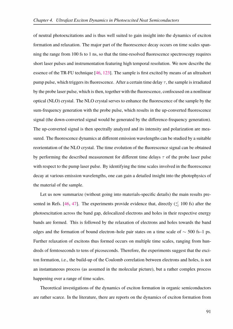
Chapter 4. Ultrafast Exciton Dynamics in Photoexcited Neat Semiconductors
of neutral photoexcitations and is thus well suited to gain insight into the dynamics of exciton
formation and relaxation. The major part of the fluorescence decay occurs on time scales span-
ning the range from 100 fs to 1 ns, so that the time-resolved fluorescence spectroscopy requires
short laser pulses and instrumentation featuring high temporal resolution. We now describe the
essence of the TR-FU technique [46, 123]. The sample is first excited by means of an ultrashort
pump pulse, which triggers its fluorescence. After a certain time delay τ , the sample is irradiated
by the probe laser pulse, which is then, together with the fluorescence, confocused on a nonlinear
optical (NLO) crystal. The NLO crystal serves to enhance the fluorescence of the sample by the
sum-frequency generation with the probe pulse, which results in the up-converted fluorescence
signal (the down-converted signal would be generated by the difference-frequency generation).
The up-converted signal is then spectrally analyzed and its intensity and polarization are mea-
sured. The fluorescence dynamics at different emission wavelengths can be studied by a suitable
reorientation of the NLO crystal. The time evolution of the fluorescence signal can be obtained
by performing the described measurement for different time delays τ of the probe laser pulse
with respect to the pump laser pulse. By identifying the time scales involved in the fluorescence
decay at various emission wavelengths, one can gain a detailed insight into the photophysics of
the material of the sample.
Let us now summarize (without going into materials-specific details) the main results pre-
sented in Refs. [46, 47]. The experiments provide evidence that, directly (. 100 fs) after the
photoexcitation across the band gap, delocalized electrons and holes in their respective energy
bands are formed. This is followed by the relaxation of electrons and holes towards the band
edges and the formation of bound electron–hole pair states on a time scale of ∼ 500 fs–1 ps.
Further relaxation of excitons thus formed occurs on multiple time scales, ranging from hun-
dreds of femtoseconds to tens of picoseconds. Therefore, the experiments suggest that the exci-
ton formation, i.e., the build-up of the Coulomb correlation between electrons and holes, is not
an instantaneous process (as assumed in the molecular picture), but a rather complex process
happening over a range of time scales.
Theoretical investigations of the dynamics of exciton formation in organic semiconductors
are rather scarce. In the literature, there are reports on the dynamics of exciton formation from
91

Chapter 4. Ultrafast Exciton Dynamics in Photoexcited Neat Semiconductors
an initial state of two opposite charges in organic semiconductors. It was typically modeled by
simulating the time evolution of empirical Hamiltonians applied to small systems, where the
effects of the lattice are not included at all or are treated classically [124, 125]. These studies
were motivated by applications in organic light-emitting diodes, whose working mechanism is
in some sense the reverse of the working mechanism of OSCs. The dynamics of light-induced
exciton formation in organic semiconductors has not received wider theoretical attention, mainly
because of the challenges related to the treatment of strong carrier–carrier and carrier–phonon
interactions. One should explicitly and simultaneously consider the interaction with the optical
field generating electronic excitations, the Coulomb interaction causing the binding of electrons
and holes into excitons, the carrier delocalization, and the carrier–phonon coupling that is re-
sponsible for relaxation processes. Apart from the treatment of the rather strong Coulomb in-
teraction, a matter of concern to the theoretical modeling is also the carrier–phonon coupling,
which is commonly considered to be quite strong in organic semiconductors. As a result, carriers
are expected to undergo strong phonon-induced renormalization and have polaronic character,
meaning that the treatment of the carrier–phonon coupling should be essentially unperturbative.
However, in Ref. [126], a microscopic treatment of the carrier–phonon coupling in a crystalline
organic semiconductor provided evidence for nonpolaronic nature of charge carriers. With this
result in mind, in this thesis, we content ourselves with the essentially perturbative treatment of
the carrier–phonon coupling that has been presented in Ch. 3. The treatment of the Coulomb
interaction in Ch. 3 effectively neglects electron–electron and hole–hole interactions, which is
a sufficiently good approximation in the low-density regime we are concentrated on. It, how-
ever, treats the electron–hole interaction, which is the most important ingredient in the exciton
formation process, properly in the low-density limit. On subpicosecond and picosecond time
scales, which are of our main interest, the effects of exciton recombination can safely be ne-
glected, since the exciton lifetime in most organic semiconductors is of the order of hundreds of
picoseconds [127]. Therefore, we are confident that the theoretical treatment introduced in Ch. 3
can provide us with meaningful insights into the dynamics of exciton formation and relaxation
on ultrafast time scales.
92

Chapter 4. Ultrafast Exciton Dynamics in Photoexcited Neat Semiconductors
4.2 Model Description
4.2.1 One-Dimensional Semiconductor Model
The exciton formation and relaxation dynamics are studied in a two-band one-dimensional semi-
conductor model. We use a tight-binding model on a one-dimensional lattice with N sites and
lattice spacing a to describe the semiconductor. Periodic boundary conditions are used. The
Hamiltonian describing interacting carriers is given as
Hc =
N−1∑
i=0
ǫc0 c†ici −
N−1∑
i=0
Jc(c†ici+1 + c†i+1ci)−N−1∑
i=0
ǫv0 d†idi +
N−1∑
i=0
Jv(d†idi+1 + d†i+1di)
+1
2
N−1∑
i,j=0
(c†ici − d†idi)Vij(c†jcj − d†jdj).
(4.1)
Operators c†i and ci (d†i and di) create and annihilate an electron (a hole) at lattice site i. It
is assumed that the carrier transfer integrals Jc, Jv are nonzero only among nearest-neighbor
pairs of sites. The Coulomb interaction is taken into account in the lowest monopole–monopole
approximation [87], and the interaction potential Vij is taken to be the Ohno potential
Vij =U
√
1 +(
|i−j|aa0
)2. (4.2)
The Ohno potential is commonly used to describe the electron–electron interaction in conju-
gated polymers [77]. U is the on-site carrier–carrier interaction, while a0 is the characteristic
length given as a0 = e2/(4πε0εrU), where εr is the static relative dielectric constant. This
form of carrier–carrier interaction is an interpolation between the on-site Coulomb interaction
U and the ordinary Coulomb potential (in which the static relative dielectric constant is taken)
e2/(4πε0εrr) when r → ∞ (see, e.g., the discussion on the effective electron–hole interaction
in Ref. [86]). The interaction with phonons is taken to be of the Holstein form, where a charge
carrier is locally and linearly coupled to a dispersionless optical mode
Hc−p =
N−1∑
i=0
gc c†ici(bi + b†i )−N−1∑
i=0
gv d†idi(bi + b†i ), (4.3)
93

Chapter 4. Ultrafast Exciton Dynamics in Photoexcited Neat Semiconductors
where the free-phonon Hamiltonian describes noninteracting oscillators localized at single lat-
tice sites
Hp =
N−1∑
i=0
~ωphb†ibi. (4.4)
Despite the fact that the carrier–phonon interaction in real materials has a more complicated
form, we choose for our numerical investigations its simplest possible form [Eq. (4.3)] capable
of providing the energy relaxation of the electronic subsystem. The interaction with the electric
field is
Hc−f = −dcvE(t)N−1∑
i=0
(dici + c†id†i), (4.5)
where dcv denotes the interband dipole matrix element.
As the system described is translationally symmetric, we can transfer to the momentum space
and obtain the same Hamiltonian as described in Eqs. (2.34)–(2.38) with the following values
of parameters:
ǫc/vk = ǫ
c/v0 − 2Jc/v cos(ka), (4.6a)
γqk1k2 = δk2,k1+qgc√N
fork1, k2 ∈ CB, (4.6b)
γqk1k2 = δk1,k2+qgv√N
fork1, k2 ∈ VB, (4.6c)
V vvccpqkl = δk+q,p+lVk−l, V vccv
plkq = 0. (4.6d)
There are exactlyN allowed values of wave vector k that are consistent with the periodic bound-
ary conditions,
k =2π
Nan, (4.7)
where n is an integer. Within the first Brillouin zone, the upper limit of n is
⌊N
2
⌋
, while its
lower limit is −⌊N
2
⌋
. We take that the signs of the transfer integrals are Jc > 0, Jv < 0. The
constant energy ǫc0 > 0, while ǫv0 < 0 is chosen so that the maximum of the valence band is
the zero of the energy scale. Vk−l is the Fourier transformation of the Ohno potential and it is
94
Chapter 4. Ultrafast Exciton Dynamics in Photoexcited Neat Semiconductors
computed numerically as
Vk =1
N2
N−1∑
i,j=0
Vij e−ika(i−j). (4.8)
The translational symmetry of our model enables us to efficiently solve the eigenvalue prob-
lem [Eq. (2.46)] that defines the exciton basis. Using Eq. (4.6), Eq. (2.46) can be rewritten as
(ǫcke − ǫvkh
)ψxkhke
−∑
k′e
Vke−k′eψxkh+ke−k′e,k
′e= ~ωxψ
xkhke
. (4.9)
Equation (4.9) shows that each exciton state x is characterized by the sumQ = kh+ke, which can
be interpreted as the center-of-mass wave vector of the electron–hole pair. The wave vectorQ can
assumeN possible values that are of the type given in Eq. (4.7). Therefore, instead of regarding
Eq. (4.9) as the eigenvalue problem of an N2 × N2 matrix, we can regard it as N independent
eigenvalue problems (one for each allowed value of Q) of matrices of dimension N × N . We
thus obtain N2 exciton eigenstates, which are counted by Q and the so-called band index ν =
0, 1, . . . , N−1. The band index enumerates the distinct eigenstates of the aforementionedN×N
matrix. WhileQ characterizes the motion of the pair as a whole, ν describes the internal motion
of the pair, see also a more general discussion in Appendix D.1. As an efficient and numerically
accurate tool to solve the eigenvalue problem embodied in Eq. (4.9), we used routines provided
by the Linear Algebra Package (LAPACK), which is a standard software library for numerical
linear algebra. In our computations,N is of the order of 100, and the solution of 100 eigenvalue
problem of matrices of dimension 100×100 takes a couple of seconds on a single processor. The
numerical complexity lies in the integration of the system of quantum kinetic equations, which
will be addressed in more detail in Sec. 4.3.
The general index of an exciton state x should be, in all practical calculations, replaced by
combination (Q, ν). This has the following consequences on the matrix elements in the exciton
basis: dipole matrix elements [Eq. (3.50)] reduce to
M(Qν) = δQ,0 dcv∑
ke
ψ(Qν)∗Q−ke,ke
, (4.10)
95

Chapter 4. Ultrafast Exciton Dynamics in Photoexcited Neat Semiconductors
whereas carrier–phonon interaction matrix elements [Eq. (3.51)] reduce to
Γq(Qν)(Q′ν′) = δQ′,Q+q
1√N
∑
ke
ψ(Qν)∗Q−ke,ke
(
gcψ(Q′ν′)Q−ke,Q′−Q+ke
− gvψ(Q′ν′)Q′−ke,ke
)
. (4.11)
Due to the translational symmetry of our model, only the dynamic variables for which the
total created wave vector is equal to the total annihilated wave vector will acquire nontrivial
values in the course of the system’s evolution. For example, from all the density matrices y(Qν),
only those with Q = 0 can have nonzero values.
Our objective is to analyze, within the framework of this relatively simple model, the charac-
teristic time scales of exciton formation and relaxation in a photoexcited semiconductor, along
with the impact that various model parameters have on these processes. Basic parameters in
our model are transfer integrals Jc and Jv (which determine bandwidths of the conduction and
valence bands), electron–phonon coupling constants gc and gv, the phonon energy ~ωph, the
dielectric constant εr, and the on-site Coulomb interaction U . We will, throughout the compu-
tations, assume for simplicity that |Jc| = |Jv| = J and gc = gv = g.
4.2.2 Parametrization of the Model Hamiltonian
As has been discussed in more detail in Ch. 1, the main differences between a typical organic and
inorganic semiconductor can be expressed in terms of bandwidths, dielectric constant, and the
carrier–phonon interaction strength, see, e.g., Ref. [6]. Namely, inorganic semiconductors are
characterized by wide bands and high value of dielectric constant (good dielectric screening),
whereas organic semiconductors have narrow bands and small value of dielectric constant (the
Coulomb interaction is poorly screened). The carrier–phonon interaction is generally stronger in
organic than in inorganic semiconductors. Having all these facts in mind, we propose two sets of
model parameters which assume values typical of an organic and inorganic semiconductor. Val-
ues of our model parameters are adjusted to material parameters of bulk GaAs for the inorganic
case and pentacene crystal for the organic case. Values of carrier–phonon coupling constants are
chosen to correspond to typical values of mobility and/or typical values of the polaron binding
energy.
96

Chapter 4. Ultrafast Exciton Dynamics in Photoexcited Neat Semiconductors
The lattice constant is fixed to a = 1 nm for both organic and inorganic parameter sets. Typ-
ical bandwidths in organic semiconductors are W ∼ 500 meV [6], which corresponds to the
transfer integral of J ∼ 125 meV in our one-dimensional model. On the other hand, inorganic
semiconductors usually exhibit bandwidths of several electronvolts [6], and we take in our cal-
culations the value of the transfer integral J = 500 meV. The dielectric constant in a typical
inorganic semiconductor is of the order of 10 and in the calculations we take the value of static
dielectric constant of GaAs εr = 12.9. For a representative value of the dielectric constant in
organic semiconductors we take εr = 3.0. The value of the on-site Coulomb interaction U is
chosen to give the correct order of magnitude for the exciton binding energy, which is calculated
numerically as the energy difference between the lowest-lying exciton state (Q = 0, ν = 0)2 and
the single-particle band gap at Q = 0, cf. Eqs. (2.75)–(2.77). For the organic parameter set,
we set U = 480 meV, which gives the exciton binding energy of around 320 meV, while for the
inorganic parameter set U = 15 meV and the corresponding exciton binding energy is roughly
10 meV.
The carrier–phonon coupling constants for the inorganic case are estimated from the mobility
values. The mobility of carriers is estimated using the relation µ = eτ/m∗, where τ is the
inelastic scattering time, e > 0 is the elementary charge, andm∗ is the effective mass of a carrier.
For cosine bands considered here, m∗ = ~2/ (2|J |a2) in the vicinity of the band extremum. The
scattering time is estimated from the expression for the carrier–phonon inelastic scattering rate
based on the Fermi’s golden rule, which around the band extremum k = 0 assumes the following
form:1
τ(k)=
g2
~|J |nph
√
1−(
cos(ka)− ~ωph
2|J |
)2, (4.12)
where nph = (eβ~ωph − 1)−1. Therefore, the carrier–phonon coupling constant in terms of the
carrier mobility reads as
g = |J |√
2ea2
~µnph
(
1−(
1− ~ωph
2|J |
)2)1/4
. (4.13)
2Here, the lowest band of exciton states is ν = 0, while the integer index of the lowest-energy Wannier excitonin Sec. 2.3.1 is n = 1.
97

Chapter 4. Ultrafast Exciton Dynamics in Photoexcited Neat Semiconductors
Table 4.1: Values of model parameters that are representative of a typical organicand inorganic semiconductor. References from which the values of material pa-rameters are extracted are indicated.
Parameter Inorganic OrganicEg (meV) 1519 [115] 2000 [130]J (meV) 500 125
εr 12.9 [115] 3.0 [6]g (meV) 25 40
~ωph (meV) 36.4 [115] 10.0 [131, 132]U (meV) 15 480
Using the value of the electron mobility in GaAs at 300 K, µe ≈ 8500 cm2/(Vs) [128], we obtain
g ≈ 25 meV.
We can also estimate the carrier–phonon coupling constants from the polaron binding energy.
As an estimate of this quantity, we use the result of the second-order weak-coupling perturbation
theory at T = 0 in the vicinity of the point k = 0 [129]:
ǫpolb (k) =g2
2|J |1
√(
cos(ka) +~ωph
2|J |
)2
− 1
. (4.14)
It is known that polaron binding energies in typical inorganic semiconductors are ǫpolb ∼ 1 meV
and we use this fact along with Eq. (4.14) to check our estimate for g from the value of mobility;
for g ≈ 25 meV, we obtain ǫpolb ≈ 2 meV. The polaron binding energies in polyacenes lie in the
range between 21 and 35 meV [17]. The value of g in the set of model parameters representative
of organic semiconductors was estimated from the polaron binding energy in pentacene, which
is around 20 meV. We obtain that g ≈ 40 meV. The values used for the organic/inorganic set of
parameters are summarized in Table 4.1.
The form of the electric field is assumed to be a rectangular cosine pulse
E(t) = E0 cos(ωct)θ(t+ t0)θ(t0 − t), (4.15)
where ωc is the central frequency of the field and θ(t) is the Heaviside step function. Time t0
is chosen large enough so that the pulse is so spectrally narrow that the notion of the central
98

Chapter 4. Ultrafast Exciton Dynamics in Photoexcited Neat Semiconductors
Table 4.2: Numbers of active density matrices in the most general case (the firsttwo columns) and the case specific to our model (the last two columns). The wavevectors appearing as arguments of the density matrices listed in the third columnassume the form given in Eq. (4.7).
General Form Total Number Specific Form Actual Numberyx N2 y(Q=0,ν) nband
yxµ+ N3 y(qν)q+ N × nband
yxµ− N3 y(−qν)q− N × nband
nxx N4 n(Qν)(Qν) N × n2band
nxxµ+ N5 n(Q−q,ν)(Qν)q+ N2 × n2band
frequency makes sense. On the other hand, the pulse should be as short as possible, so that after
its end we observe the intrinsic dynamics of our system, the one which is not accompanied by
the carrier generation process, but merely shows how initially generated populations are redis-
tributed among various states. Trying to reconcile the aforementioned requirements, we choose
t0 = 250 fs. The amplitude of the electric field E0 and the interband dipole matrix element dcv
are chosen so that we stay in the low-density regime; particularly, we choose them so that the
corresponding Rabi frequency ~ωR = dcvE0 assumes the value of 0.2 meV, which is smaller
than any energy scale in our problem and ensures that the excitation is weak.
4.3 Numerical Results
In order to quantitatively study the process of exciton formation during and after a pulsed excita-
tion of a semiconductor, we solve the system of quantum kinetic equations for electronic density
matrices yx and nxx, and their single-phonon-assisted counterparts [Eqs. (3.48), (3.49), (3.66),
(3.67), and (3.68) supplemented with Eqs. (3.79) and (3.81)] using the fourth-order Runge–Kutta
algorithm [133]. The model described in Sec. 4.2.1 features N2 exciton states and N phonon
modes in total. The total numbers of density matrices of various types are presented in the second
column of Table 4.2. However, in actual computations, the number of active density matrices is
further reduced by combining the translational symmetry of the model with the fact that the cen-
tral frequency of the excitation and the thermal energy crucially determine the number of exciton
states that can be involved in the ultrafast dynamics. For the sake of convenience in numerical
implementation, in our computations, we do not select a certain number of lowest-lying exciton
99
Chapter 4. Ultrafast Exciton Dynamics in Photoexcited Neat Semiconductors
states, but deal only with whole exciton bands, and consider only nband lowest-lying bands. For
the given central frequency ωc of the excitation, we take into account all the bands whose minima
lie below ~ωc + αkBT , where α ∼ 5 is a numerical constant. We have explicitly checked that
employing higher values of α does not significantly change our numerical results. The forms of
the active density matrices that take into account the translational symmetry of our model are
summarized in the third column of Table 4.2. The fourth column of Table 4.2 lists the numbers
of various types of density matrices that are actually considered in computations. In the com-
putations whose results are presented in Sec. 4.3.1, we take N = 101, while nband is typically
around 25, so that the total number of single-phonon-assisted density matrices n(Q−q,ν)(Qν)q+
typically ranges between 5 × 10⁶ and 107. Since the numbers of the active density matrices of
other types are much smaller, see the fourth column of Table 4.2, the system of mutually coupled
differential equations that we have to solve contains around ten million equations in total. It is
then clear that high performance computing (HPC) resources play a crucial role in solving such
a large system of equations in a reasonable amount of time. Our computations are performed on
the PARADOX supercomputing facility at the Scientific Computing Laboratory of the Institute
of Physics Belgrade. We construct our own C program that can be run in parallel on a num-
ber of processors. The communication between different processors is accomplished by using
Message Passing Interface (MPI) routines. In order to keep this communication at a reasonable
level, at each time step, all of the processors keep information about all of the active density
matrices.3 The parallelization scheme that we adopt, therefore, does not involve the reduction in
size of the memory space used by individual processors, but rather reduces the execution time
by evenly dividing numerical effort between processors. Namely, each of the processors effec-
tively computes time evolution of only a portion of the total number of each of the five types
of active density matrices listed in Table 4.2, while the values of all the other density matrices
are set to zero. This is schematically depicted in Fig. 4.1, in which processor Pi computes only
portion i (in gray) of the active density matrices. After the calculations in one time step have
3Since one time step in fourth-order Runge–Kutta method consists of four substeps, this also holds in individualsubsteps.
100

Chapter 4. Ultrafast Exciton Dynamics in Photoexcited Neat Semiconductors
0 0 0 0 0 0
0 0 0 0 0 0
0 0 0000
. . . . . . . . . . . .
. . . . . . . . .
. . . . . . . . . . . .
. . .
. . .
. . .
. . .
P1
P2
PN
Portion 1 Portion 2 Portion N
Figure 4.1: Schematic view of the parallelization scheme implemented in our ownC program that performs integration of the system of quantum kinetic equations.Each row shows the memory space allocated by individual processors. Columnsshow the division of the memory space into portions. In row i, only the densitymatrices in the portion in gray (Portion i) are actually propagated in time by pro-cessor Pi.
been completed, a simple column-wise summation of the results obtained on individual proces-
sor ensures that all of the processors have information on all of the active density matrices. Our
computations were typically performed on 64 or 128 CPU cores. Regarding the time step for
numerical integration of the system of quantum kinetic equations, after separating out the fast
free evolution of coherent quantities yx and yxµ± [see Eq. (3.93)], the equations for quantities
yx, yxµ± , nxx, and nxxµ+ can be integrated with the same time step ∆t = 0.8 fs. Therefore,
computing 5 fs of exciton dynamics requires 6250 time steps. In the computations whose results
are presented in Sec. 4.3.1, each time step lasts for around 2.5 s, meaning that 5 fs of exciton
dynamics is typically computed within ca. 5 hours.
If not explicitly states otherwise, the computations are performed for the temperature T =
300 K and the central frequency of the pulse equal to the single-particle gap (~ωc = Eg).
The exciton state characterized by pair (Q, ν) is considered bound (unbound) if its energy
~ω(Qν) is smaller (larger) than the smallest (with respect to ke) single-particle energy difference
ǫcke − ǫvQ−ke[130]. The equation of the boundary line that separates bound from unbound pair
states reads as
ǫsep(Q) = ǫc0 − ǫv0 − 2√
(Jc)2 + (Jv)2 − 2JcJv cos(Qa). (4.16)
An unbound exciton may be considered as (quasi)free electron and hole, so this way it is possible
to distinguish between bound excitons and free carriers.
101

Chapter 4. Ultrafast Exciton Dynamics in Photoexcited Neat Semiconductors
The exciton formation and the initial stages of exciton relaxation are examined by following
the decay of the coherent pair occupation
Ncoh =∑
ν
|y(Q=0,ν)|2, (4.17)
and the build-up of the total number of incoherent bound excitons
Nincoh,b =∑
x∈bound
nxx. (4.18)
The quantity Nincoh,b represents the number of truly bound electron–hole pairs that exist even
after the optical field has vanished and, as such, is the direct measure of the efficiency of the ex-
citon formation process. We will, when useful, also consider the number of incoherent excitons
in a particular band ν,
Nincoh,ν =∑
Q
n(Qν)(Qν). (4.19)
The quantities Nincoh,b and Nincoh,ν will be normalized to the total number of excitons Ntot
defined in Eq. (3.54), which is conserved after the excitation.
4.3.1 Organic Set of Parameters
We start this section by an overview of the properties of the exciton spectrum shown in Fig. 4.2(a)
that will be relevant for further discussion of the exciton formation process. The lowest band of
exciton states is energetically well separated from the rest of the spectrum, the energy separation
between the minima of the bands ν = 0 and ν = 1 being around 200 meV, which is much
larger than both the value of kBT at room temperature and the phonon energy in our model (see
Table 4.1). As a consequence, downward transitions that end on the lowest exciton band start
almost exclusively from the states on ν = 1 band and an exciton, which is at some instant in a
state on the ν = 0 band, cannot be scattered to an unbound exciton state.
We briefly comment on the size of the exciton for these values of model parameters. From
the exciton wave function ψ(Qν)Q−ke,ke
in k space, we can obtain the exciton wave function in real
102

Chapter 4. Ultrafast Exciton Dynamics in Photoexcited Neat Semiconductors
Energy (eV
)(a)
(b)
0 20-200
0.1
0.2
0.3
0.4
0 0.5-0.5 1-11.6
1.8
2
2.2
2.4
2.6
2.8
3
40-40
Figure 4.2: (a) Exciton spectrum for the organic set of parameters. Dots repre-sent individual exciton states (Q, ν), while thick red line is the boundary betweenbound and unbound exciton states computed using Eq. (4.16). (b) Squared mod-ulus of the wave function that describes the relative motion of an electron–holepair [Eq. (4.21)] calculated for different states (Q = 0, ν). Mean electron–holeseparations in these states are 0.7 a (ν = 0), 2.5 a (ν = 1), 4.6 a (ν = 2), and 7.8 a(ν = 3). Computations are performed for N = 101.
103

Chapter 4. Ultrafast Exciton Dynamics in Photoexcited Neat Semiconductors
space by performing the Fourier transformation [compare to Eq. (2.69)]
ψ(Qν)rhre
=∑
ke
ei(Q−ke)rheikereψ(Qν)Q−ke,ke
= eiQ(re+rh)/2∑
ke
e−i(Q−2ke)(re−rh)/2ψ(Qν)Q−ke,ke
.
(4.20)
The exciton wave function in real space is a product of the plane wave that describes the motion
of the center of mass with the wave vector Q and the wave function of the relative motion of an
electron and a hole:
ψrel(Qν) =
∑
ke
e−i(Q−2ke)(re−rh)/2ψ(Qν)Q−ke,ke
. (4.21)
The latter part is directly related to the exciton size. We calculated squared modulus of the wave
function of the relative motion of a pair for states (Q = 0, ν) in various bands. The result is
shown in Fig. 4.2(b). It is clearly seen that an electron and a hole are tightly bound in these states
and their relative separations are of the order of lattice constant, which is the typical value for the
exciton radius in organic semiconductors. We point out that this does not mean that an exciton
is localized; due to the translational symmetry of our system, it is delocalized over the whole
lattice, as described by the plane-wave factor in the total wave function of a pair. Moreover, we
note that the system size N = 101 is large enough for the results to be numerically accurate, as
it is much larger than the typical size of the exciton in a bound state.
Let us first discuss the exciton formation process for different central frequencies of the ex-
citing pulse. We have considered central frequencies in resonance with (Q = 0, ν = 1) state,
(Q = 0, ν = 2) state, single-particle gap Eg, and the central frequency which is 100 meV above
the band gap. As can be noted from Fig. 4.3, raising the central frequency of the laser field leads
to lower relative number of incoherent bound excitons. Namely, the higher is the central fre-
quency, the higher (in energy) are the bands in which the initial coherent exciton populations are
created and the slower is the conversion of these coherent populations to incoherent populations
in lower exciton bands. However, in the long-time limit, the relative number of incoherent bound
excitons should not depend on the central frequency of the laser, but tend to the value predicted
by the Maxwell–Boltzmann distribution, which is above 99%. Such a high value is due to the
104

Chapter 4. Ultrafast Exciton Dynamics in Photoexcited Neat Semiconductors
Time (ps)0 1 2 3 4 5
0
0.2
0.4
0.6
0.8
1
Figure 4.3: Time dependence of the relative number of incoherent bound excitonsfor different central frequencies of the pulse. The dashed vertical line marks theend of the pulsed excitation.
large energy separation between the lowest exciton band and the rest of the spectrum. We can
thus infer, based on Fig. 4.3, that the semiconductor dynamics right after the pulsed excitation
shows highly nonequilibrium features. Relaxation towards equilibrium occurs on a time scale
longer than the picosecond one.
Next, we consider the dependence of the exciton formation process on temperature. The
temperature enters our model only through phonon numbers nph. The overall behavior of the
relative number of incoherent bound excitons for different temperatures is presented in Fig. 4.4.
During the pulse, the relative number of incoherent bound excitons is highest for T = 300 K
and lowest for T = 100 K, which is the consequence of the fact that scattering processes from
higher-lying exciton bands (in which initial coherent exciton populations are created and which
are situated both in the pair continuum and below it) towards lower-lying exciton bands are most
efficient at T = 300 K. After the generation of carriers has been completed, phonon-mediated
processes lead to the redistribution of created incoherent excitons among different exciton states
and the relative number of incoherent bound excitons increases with decreasing the temperature,
which is the expected trend. In the inset of Fig. 4.4 we also note that the relative number of in-
coherent bound excitons after the pulse experiences an initial growth followed by a slow decay
at T = 300 K, whereas at T = 100 K it monotonically rises. The initial growth at T = 300 K
is attributed to downward scattering processes, but since at this temperature upward scattering
105

Chapter 4. Ultrafast Exciton Dynamics in Photoexcited Neat Semiconductors
0 1 2 3 4 5Time (ps)
0
0.2
0.4
0.6
0.8
1
1 2 3 4 50.75
0.8
0.85
0.9
Figure 4.4: Time dependence of the relative number of incoherent bound excitonsfor different temperatures. The dashed vertical line marks the end of the pulsedexcitation. The inset shows the portions of the same curves after the pulse.
events cannot be neglected, the following slow decay is due to the fact that some exciton bands
situated well below the pair continuum (bands ν = 1, 2, 3) lose excitons both by downward scat-
tering and upward scattering to exciton states which are near to or belong to the pair continuum
[see Figs. 4.5(a) and 4.5(b)]. At T = 100 K, these upward processes are much less probable than
downward processes, thus the decay of the relative number of incoherent bound excitons is not
observed; in Figs. 4.5(c) and 4.5(d) we see that lowest exciton bands (ν = 0, 1, 2) gain excitons,
whereas bands that are near to or belong to the pair continuum (ν = 9, 11, 13 ,15) lose exci-
tons. The population of the lowest exciton band ν = 0 continually grows at all the temperatures
studied, due to the large energetic separation between this band and the rest of the spectrum.
We briefly comment on the behavior of the number of coherent excitons Ncoh and its tem-
perature dependence. Right after the start of the pulse, coherent excitons comprise virtually the
total exciton population, see Fig. 4.6. Due to the carrier–phonon interaction, the relative number
of coherent excitons decays during the pulse, so that at its end coherent excitons comprise around
1% of the total exciton population. The conversion from coherent to incoherent populations is
thus almost completed by the end of the pulse. From the inset of Fig. 4.6, we note thatNcoh/Ntot
exhibits a very fast decay after the pulse has vanished. The time it takes for the ratioNcoh/Ntot to
decay ten times is of the order of 50 fs or less. Therefore, we infer that the transformation from
coherent to incoherent exciton populations takes place on a 50-fs time scale. Based on Fig. 4.6,
106
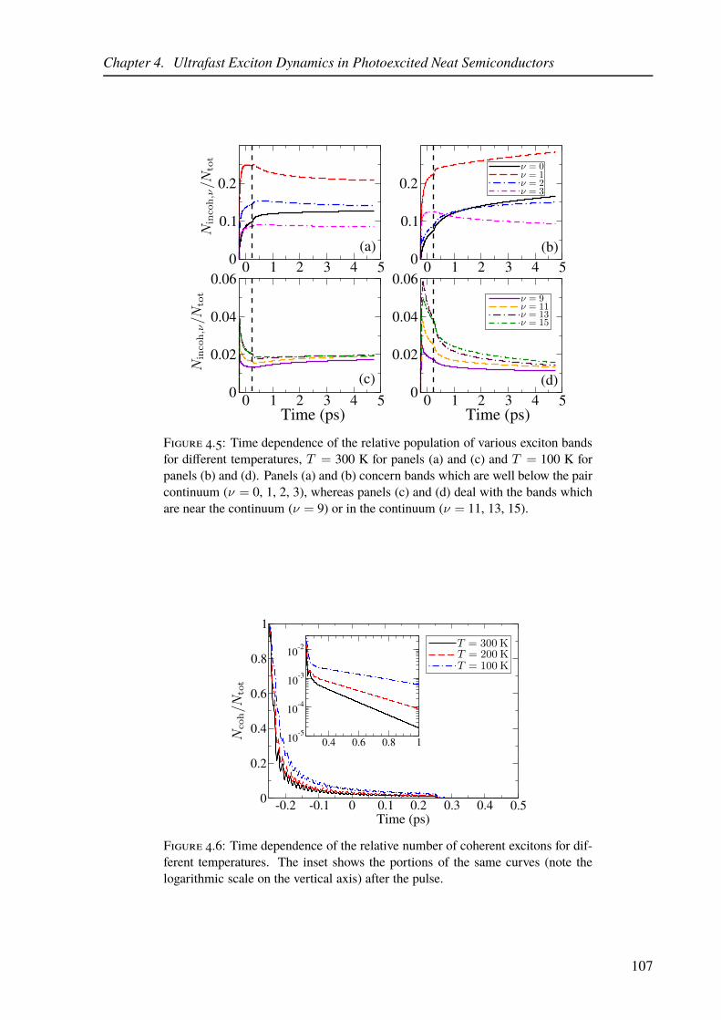
Chapter 4. Ultrafast Exciton Dynamics in Photoexcited Neat Semiconductors
0 1 2 3 4 50
0.1
0.2
0 1 2 3 4 50
0.1
0.2
0 1 2 3 4 5Time (ps) Time (ps)
0
0.02
0.04
0.06
0 1 2 3 4 50
0.02
0.04
0.06
(a) (b)
(c) (d)
Figure 4.5: Time dependence of the relative population of various exciton bandsfor different temperatures, T = 300 K for panels (a) and (c) and T = 100 K forpanels (b) and (d). Panels (a) and (b) concern bands which are well below the paircontinuum (ν = 0, 1, 2, 3), whereas panels (c) and (d) deal with the bands whichare near the continuum (ν = 9) or in the continuum (ν = 11, 13, 15).
-0.2 -0.1 0 0.1 0.2 0.3 0.4 0.50
0.2
0.4
0.6
0.8
1
0.4 0.6 0.8 110-5
10-4
10-3
10-2
Time (ps)
Figure 4.6: Time dependence of the relative number of coherent excitons for dif-ferent temperatures. The inset shows the portions of the same curves (note thelogarithmic scale on the vertical axis) after the pulse.
107

Chapter 4. Ultrafast Exciton Dynamics in Photoexcited Neat Semiconductors
0 1 2 3 4 50
0.2
0.4
0.6
0.8
1
1 2 3 4 5
0.75
0.8
0 1 2 3 4 5Time (ps)
0
0.05
0.1
(a)
(b)
Figure 4.7: Time dependence of: (a) the relative number of incoherent boundexcitons, (b) the relative number of incoherent excitons in the ν = 0 band, forvarious values of g. The inset in the panel (a) shows the portions of the samecurves after the pulse.
we also note that the lower is the temperature, the slower is the transformation from coherent to
incoherent exciton populations, which is the expected trend.
We continue our investigation by examining the effects that changes in the carrier–phonon
coupling constant g have on the exciton formation process. Since increasing (lowering) g in-
creases (lowers) semiclassical transition rates, just as increasing (lowering) T does, the changes
in g and T should have, in principle, similar effects on the exciton formation process. Consider-
ing first the relative number of incoherent bound excitons, whose time dependence for different
values of g is shown in Fig. 4.7(a), we note that, after the end of the pulse, it increases with
decreasing g. However, during the pulse, higher values of g lead to more incoherent bound
excitons, as is expected since scattering processes which populate low-energy states are more
108

Chapter 4. Ultrafast Exciton Dynamics in Photoexcited Neat Semiconductors
0 1 2 3 4 5Time (ps)
0
0.2
0.4
0.6
0.8
1
1 2 3 4 5
0.6
0.8
Figure 4.8: Time dependence of the relative number of incoherent bound excitonsfor various values of U . The inset shows the portions of the same curves after thepulse.
intensive for larger g. We also show the time dependence of the relative number of excitons in
ν = 0 band in Fig. 4.7(b). It is observed that the lower is g, the lower is the number of excitons in
the lowest exciton band. This is due to the fact that populations on the lowest band are generated
mainly via scattering processes from the ν = 1 band and these processes are less efficient for
smaller g.
We conclude this section by studying the effects that changes in the on-site Coulomb interac-
tionU have on the process of exciton formation. Changing U has profound effects on the exciton
spectrum. Exciton binding energy lowers with lowering U along with the energy separation be-
tween the band ν = 0 and the rest of the spectrum. We studied the impact of U on the exciton
formation process for three values of U , U = 480, 240, and 48 meV, for which the exciton bind-
ing energy is ∼ 320, ∼ 175, and ∼ 40 meV, respectively. Lowering U lowers the relative number
of incoherent bound excitons, as is shown in Fig. 4.8. Smaller energy separation between the
lowest exciton band and the rest of the spectrum means that phonon-mediated transitions which
start/end on the band ν = 0 can end/start not predominantly on the band ν = 1, but also on
higher exciton bands, which, for lower U , are more certain to belong to the electron–hole pair
continuum than to the part of the spectrum that contains bound pair states. Thus, the lower is
U , the more likely are the dissociation processes in which an exciton, initially in a bound state,
after a phonon-mediated transition ends in an unbound pair state, which explains the observed
109
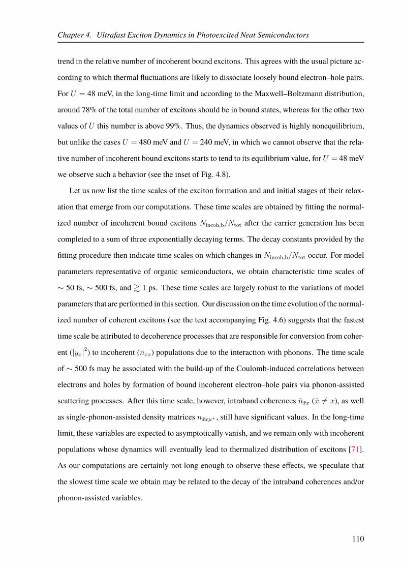
Chapter 4. Ultrafast Exciton Dynamics in Photoexcited Neat Semiconductors
trend in the relative number of incoherent bound excitons. This agrees with the usual picture ac-
cording to which thermal fluctuations are likely to dissociate loosely bound electron–hole pairs.
For U = 48 meV, in the long-time limit and according to the Maxwell–Boltzmann distribution,
around 78% of the total number of excitons should be in bound states, whereas for the other two
values of U this number is above 99%. Thus, the dynamics observed is highly nonequilibrium,
but unlike the cases U = 480 meV and U = 240 meV, in which we cannot observe that the rela-
tive number of incoherent bound excitons starts to tend to its equilibrium value, for U = 48 meV
we observe such a behavior (see the inset of Fig. 4.8).
Let us now list the time scales of the exciton formation and and initial stages of their relax-
ation that emerge from our computations. These time scales are obtained by fitting the normal-
ized number of incoherent bound excitons Nincoh,b/Ntot after the carrier generation has been
completed to a sum of three exponentially decaying terms. The decay constants provided by the
fitting procedure then indicate time scales on which changes in Nincoh,b/Ntot occur. For model
parameters representative of organic semiconductors, we obtain characteristic time scales of
∼ 50 fs, ∼ 500 fs, and & 1 ps. These time scales are largely robust to the variations of model
parameters that are performed in this section. Our discussion on the time evolution of the normal-
ized number of coherent excitons (see the text accompanying Fig. 4.6) suggests that the fastest
time scale be attributed to decoherence processes that are responsible for conversion from coher-
ent (|yx|2) to incoherent (nxx) populations due to the interaction with phonons. The time scale
of ∼ 500 fs may be associated with the build-up of the Coulomb-induced correlations between
electrons and holes by formation of bound incoherent electron–hole pairs via phonon-assisted
scattering processes. After this time scale, however, intraband coherences nxx (x 6= x), as well
as single-phonon-assisted density matrices nxxµ+ , still have significant values. In the long-time
limit, these variables are expected to asymptotically vanish, and we remain only with incoherent
populations whose dynamics will eventually lead to thermalized distribution of excitons [71].
As our computations are certainly not long enough to observe these effects, we speculate that
the slowest time scale we obtain may be related to the decay of the intraband coherences and/or
phonon-assisted variables.
110

Chapter 4. Ultrafast Exciton Dynamics in Photoexcited Neat Semiconductors
-1 -0.5 0 0.5 11.5
2
2.5
3
3.5
4
4.5
5
5.5
Energy (eV
)
-50 0 500
0.01
0.02
0.03
0.04
(a)
(b)
-0.1 0 0.11.5
1.51
1.52
1.53
1.54
1.55
Figure 4.9: (a) Exciton spectrum for the inorganic set of parameters. Dots repre-sent individual exciton states (Q, ν), while thick red line is the boundary betweenbound and unbound exciton states computed using Eq. (4.16). The inset shows thesame spectrum in the range of energies around the single-particle gap. (b) Squaredmodulus of the wave function which describes the relative motion of an electron–hole pair [Eq. (4.21)] calculated for different states (Q = 0, ν). Mean electron–hole separations are 9.1 a (ν = 0) and 29.4 a (ν = 1), while states (Q = 0, ν = 2)and (Q = 0, ν = 3) are not bound. Computations are performed for N = 151.
4.3.2 Inorganic Set of Parameters
Here, we investigate the exciton formation process in the case when material parameters assume
values typical of inorganic semiconductors, i.e., relatively large bandwidths, large dielectric con-
stant (weak Coulomb interaction), and weak carrier–phonon interaction. The exciton spectrum
is shown in Fig. 4.9(a). We see that almost all exciton bands belong to the pair continuum, except
for a couple of lowest bands, which is more clearly seen in the inset of Fig. 4.9(a). This is an en-
tirely different situation from the one that we encounter for the organic set of parameters, where
large energy separation of the lowest exciton band from the rest of the spectrum was crucial to
111

Chapter 4. Ultrafast Exciton Dynamics in Photoexcited Neat Semiconductors
understand the exciton formation process. As a consequence, excitons in bound states are likely
to scatter to states in the pair continuum, in contrast to the situation for the model parameters
representative of an organic semiconductor.
Having noted the important characteristics of the exciton spectrum, we move on to comment
briefly on the exciton size for the inorganic set of parameters. We plot in Fig. 4.9(b) the squared
modulus of the wave function of the relative motion of the pair, which is defined in Eq. (4.21).
We note that for the inorganic set of parameters, electron and hole are not as tightly bound
as for the organic set of parameters, which is in accord with the fact that excitons in a typical
inorganic semiconductor have large radii, typically of the order of 10 lattice constants [86].
From Fig. 4.9(b), it is also clear that, if we are to see the lowest exciton state (Q = 0, ν = 0) as
a bound pair, we should take the system size N & 120. We opt for N = 151 because this value
makes a good compromise between the minimal size of the system needed for the results to be
numerically accurate and the computational time.
For the inorganic set of parameters, we note that incoherent unbound excitons comprise the
major part of the total exciton population [see Fig. 4.10(a)], which is different from the case
when model parameters assume values representative of an organic semiconductor, when exci-
tons in bound states prevail. Considering an unbound exciton as quasifree electron and hole, we
interpret the last observation in the following manner: after an optical excitation of an organic
semiconductor, (strongly) bound electron–hole pairs (excitons) are mainly generated, whereas in
the case of an inorganic semiconductor an optical excitation predominantly generates (quasi)free
charges. In Fig. 4.10(a), we also note that for higher central frequency of the laser field, the rel-
ative number of bound excitons is lower. However, in the long-time limit the number of incoher-
ent bound excitons should assume the value predicted by the Maxwell–Boltzmann distribution,
which is around 36.5%, irrespectively of the central frequency of the pulse. The values of the
relative number of incoherent bound excitons at the end of our computations do not strongly
deviate from the value predicted by the Maxwell–Boltzmann distribution, in contrast to the situ-
ation for the organic set of parameters, where this deviation was more pronounced (see Fig. 4.3).
It can thus be inferred that nonequilibrium features of the semiconductor dynamics after a pulsed
excitation are more pronounced for the organic than for the inorganic set of parameters.
112
Chapter 4. Ultrafast Exciton Dynamics in Photoexcited Neat Semiconductors
0 1 2 3 4 50
0.1
0.2
0.3
0.4
0.5
(a)
(b)
0 1 2 3 4 5Time (ps)
0
0.1
0.2
0.3
0.4
0.5
Figure 4.10: (a) Time dependence of the relative number of incoherent bound ex-citons for the excitation resonant with the single-particle gap Eg and the one thatis 100 meV above it. The temperature in both cases is T = 300 K. (b) Time de-pendence of the relative number of incoherent bound excitons for various tempera-tures. The central frequency of the laser pulse is 100 meV above the single-particlegap.
113

Chapter 4. Ultrafast Exciton Dynamics in Photoexcited Neat Semiconductors
Finally, we comment on the temperature dependence of the exciton formation process for the
excitation whose central frequency is 100 meV above the single-particle gap. The lower is the
temperature, the higher is the relative number of the incoherent bound excitons [see Fig. 4.10(b)].
During the pulse, higher temperature leads to higher relative number of incoherent bound exci-
tons, which has already been explained in the section dealing with the organic set of parameters.
The long-time limit values of the relative number of incoherent bound excitons are 44.7% for
T = 200 K and 62.7% for T = 100 K. In all three cases, the dynamics is highly nonequilibrium,
but it displays the trend of a slow, but monotonic, approach towards the equilibrium.
4.4 Discussion and Significance of Our Results
We perform an investigation of exciton dynamics taking place on picosecond time scales follow-
ing a pulsed excitation of the model semiconductor. Despite the fact that our Hamiltonian does
not include the effects of disorder that are present in real materials and uses an oversimplified
form of the carrier–phonon interaction, the time scales of exciton formation and relaxation pro-
cesses that we obtain using the organic parameter set are consistent with experimental data on
conjugated polymer-based materials [46, 47]. The formation of strongly bound excitons is char-
acterized by multiple time scales that are concurrent with the time scale of the electron transfer
in most efficient D/A OSCs. In particular, our results indicate that, if the charge transfer from the
photoexcited donor to the acceptor took place on ∼ 100 fs time scales after the photoexcitation,
it would predominantly occur from higher-lying donor exciton states, prior to the formation of
strongly bound donor excitons, which we find to occur on a∼ 500-fs time scale. In this sense, our
results may be considered to support the hypothesis put forward by Heeger and coworkers [33],
according to which the ultrafast charge transfer in most efficient D/A blends is possible because
it takes place before the formation of strongly bound donor excitons.
Instead of focusing on details of one particular material system, we work with the model
Hamiltonian whose parameters have clear physical interpretation and can be varied, which en-
ables us to identify the influence of different physical effects on relevant time scales. We find that
the exciton formation strongly depends on the central frequency of the excitation, higher-energy
114

Chapter 4. Ultrafast Exciton Dynamics in Photoexcited Neat Semiconductors
excitations leading to more free carriers on picosecond time scales. Stronger carrier-phonon and
carrier-carrier couplings promote more efficient binding of electrons and holes into excitons. As
the temperature is decreased, the relative participation of strongly bound excitons in the total
exciton population increases.
115

Chapter 5
Origin of Space-Separated Charges in
Photoexcited Organic Heterojunctions on
Ultrafast Time Scales
The aim of this chapter is to unveil the fundamental physical mechanisms behind the experimen-
tally observed presence of spatially separated charges on subpicosecond time scales following
the photoexcitation of the most efficient D/A OSCs. As has been described in Ch. 1, these exper-
imental findings challenge the conventional picture of light-to-charge conversion in OSCs and
call for its amendments. We start this chapter with an overview (Sec. 5.1) of recent experimental
and theoretical activities that have influenced the topic of our interest. Our results regarding
subpicosecond exciton dynamics at photoexcited D/A heterojunctions are presented in Secs. 5.2
and 5.3, whose content is based on our publication [134]. Section 5.4 introduces our theoretical
treatment of ultrafast transient absorption spectroscopy, which is followed by the discussion of
the differential transmission signal computed by using the expression we derive. The results of
Sec. 5.4 were also disseminated in Ref. [134].
5.1 Experimental and Theoretical Background
Here, we provide an overview of the experimental and theoretical results that are relevant for
the topic of ultrafast charge separation at all-organic D/A heterointerfaces. The manner of the
presentation of the experimental results is similar to that in Refs. [40, 135].
116

Chapter 5. Origin of Ultrafast Charge Separation
5.1.1 Overview of Recent Experimental Results
The authors of Ref. [35] performed one of the pioneering TA experiments in the femtosecond
time regime on a conjugated polymer/fullerene blend. They succeeded in time-resolving the
photoinduced electron transfer from the excited polymer onto the fullerene with time resolution
of the order of 10 fs. Basically, the blend is first excited by a pump pulse, and thus created
nonequilibrium state of the blend is examined by comparing the absorption spectrum of the
pumped blend to the absorption spectrum of the blend in equilibrium. This comparison is per-
formed at various times after the action of the pump pulse by exposing the sample to a probe
pulse. The central experimental quantity, the DTS, may be resolved in time and/or frequency
domain, providing one with a wealth of information on photophysical processes in the blend.
A more detailed discussion of this experimental technique is deferred for Sec. 5.4. The charge
transfer was observed to be ultrafast (∼ 45 fs), but the nature of its product (whether it pro-
duces the strongly bound CT state or free charge carriers), as well as its physical mechanism,
remained unclear. Later on, time-resolved TA experiments on the blend of the low-band-gap
polymer PCPDTBT and the fullerene suggested that free carriers can be generated directly from
the initial donor excitons in less than 200 fs following the photoexcitation [27]. On the same
time scale, the electron transfer may also produce an electron–hole pair in the intermediate CT
state, which converts to long-lived free carriers in less than 10 ps. Similar conclusions were also
obtained in the P3HT/PCBM blend [136] by employing the same experimental technique.
The study by Bakulin et al. [48] shed new light on the experimentally observed presence of
free charge carriers on subpicosecond time scales after photoexcitation. The authors suggest that
the long-range charge separation in OSCs is facilitated by charge delocalization. In essence, the
presence of high-energy (“hot”) CT states, which feature quite good charge delocalization, may
enable a conversion of the initial donor exciton into a pair of free charges via a “hot” CT state, see
the separation pathway outlined by arrows (1) and (4) in Fig. 5.1, without involving the strongly
bound and localized interfacial CT state. Their proposal is based on the experimental results
obtained on a variety of material combinations by using the so-called pump–push photocurrent
technique. The blend is first excited by visible light, see the black bolt in Fig. 5.1, and, as a result,
117

Chapter 5. Origin of Ultrafast Charge Separation
"hot" CT states(1)
(2) (3)
(4)
stronglybound
CT states
free charges
ground state
Figure 5.1: Schematic view of ultrafast optical experiments performed by Bakulinet al. [48]. An excitation by visible light (black bolt) generates donor excitons.Upon ultrafast electron transfer [arrow (1)], excitons in “hot” CT states are pro-duced, which may either escape to the manifold of free-charge states [arrow (4)],or exhibit relaxation towards the strongly bound CT state [arrow (2)]. An infraredpush pulse [arrow (3)] then reexcites excitons from the strongly bound CT stateto “hot” CT states and provides them with another opportunity to separate [arrow(4)].
donor excitons, strongly bound CT excitons [see arrows (1) and (2)], and free carriers capable
of producing photocurrent [see arrows (1) and (4)] are generated. The blend is then exposed
to an infrared push pulse, whose frequency is tuned to the difference between the energies of
the initially excited donor state and the strongly bound CT state, see arrow (3) in Fig. 5.1. In
other words, the push pulse is supposed to reexcite an exciton in the strongly bound CT state to a
higher-energy CT state that is in some sense similar to the CT state formed right after the electron
transfer from the donor to the acceptor, see arrow (1) in Fig. 5.1. The change in the photocur-
rent induced by the push pulse in registered as a function of the delay between pump and push
pulses. When the push pulse arrives immediately after the pump pulse, a sharp increase in the
photocurrent (occurring within ∼ 200 fs) is observed. This sharp rise is interpreted to originate
from strongly bound CT excitons that, under the action of the push pulse, are reexcited in the CT
exciton manifold to “hot” CT states, giving them another chance to separate, see arrows (3) and
(4) in Fig. 5.1. In other words, strongly bound CT states, which are reached by the relaxation of
the initial “hot” CT population, constitute an important loss channel, whereas delocalized “hot”
CT states can separate with high efficiency. Complementary atomistic simulations revealed that
“hot” CT states are characterized by good hole delocalization along polymer chains.
118

Chapter 5. Origin of Ultrafast Charge Separation
(a) (b)
+ + + + +pump
probeprobe
80 fs
1 ps
DA
pump
probe
SHG signal
groundstate
donorstate
CT
Figure 5.2: Schematic view of ultrafast optical experiments performed byJailaubekov et al. [37]. (a) Time-resolved second harmonic generation. ECT
denotes the electric field created by separating charges, while ωpr is the probefrequency. (b) Time-resolved two-photon photoemission spectroscopy. Ultrafastcharge transfer from the initial donor state toward a “hot” CT state occurs in∼ 80 fsafter pumping, while the relaxation of “hot” excitons takes place on a picosecondtime scale.
The results of Ref. [48] suggest that a successful charge separation via “hot” CT states has to
occur prior to the relaxation of the initial CT excitons to localized and strongly bound CT states.
The ultrafast charge separation and the relaxation of CT excitons are thoroughly examined by
Jailaubekov et al. in Ref. [37]. The formation of CT excitons is studied on the well-defined het-
erojunction between copper phthalocyanine (CuPc) and fullerene (C60) by employing the time-
resolved second harmonic generation (TR-SHG), whose principal scheme is depicted Fig. 5.2(a).
The TR-SHG follows the emergence of the transient interfacial electric field ECT resulting from
charge separation at the D/A interface. The ultrashort pump laser pulse generates excitons in
the CuPc layer, and, after a time delay, the probe pulse (whose frequency ωpr is different from
the frequency of the pump pulse) is applied to the sample. As charges separate, the electric
field they create produces a signal at the second harmonic 2ωpr of the probe frequency, and this
signal is recorded as a function of the pump–probe delay. The rise-time of the TR-SHG signal
gives information on the time scale on which charges separate. The experimental results point
towards an extremely fast (. 100 fs) charge separation following the direct excitation of the bulk
CuPc. A more detailed investigation of the population dynamics and energetics of exciton states
on femtosecond time scales is performed by using the time-resolved two-photon photoemission
spectroscopy, see Fig. 5.2(b). The pump pulse generates excitons in CuPc, while the probe pulse
causes photoemission of electrons from exciton states. Based on an analysis of the kinetic en-
ergy of the photoelectrons thus obtained, one can identify the nature of the photoexcited state
119

Chapter 5. Origin of Ultrafast Charge Separation
strongly boundCT state
"hot" CT states
free charges
ground state
donor
stat
es
recombination
Figure 5.3: Summary of the photophysical pathways obtained by Grancini etal. [36] along which initially generated donor excitons are converted into freecharges. Each pathway contains information on time scales of processes involved.Solid black arrows represent transitions of donor excitons into the CT manifold,while the conversion of CT excitons into free charges is represented by solid red ar-rows. Dashed blue arrows denote direct pathways from donor to free-charge states.The recombination of the strongly bound CT state is represented by dashed blackarrow. Adapted with permission from Springer Customer Service Centre GmbH:Springer Nature, Nature Materials, Ref. [36] c© (2013).
from which the electron has been emitted. The “hot” CT excitons produced in ∼ 80 fs after the
dissociation of CuPc excitons are observed to relax within∼ 1 ps to the strongly bound CT state.
The authors propose that, on a picosecond time scale following the excitation by the pump, there
is a competition between free-carrier generation via weakly bound and delocalized “hot” CT
states and their relaxation towards strongly bound and localized CT states. This relaxation sets
the time limit for efficient charge separation at organic D/A interfaces, which is ultimately aided
by carrier delocalization.
Similar conclusions have emerged from the study by Grancini et al. [36], who performed
ultrafast TA measurements to examine the very first stages of free-charge generation in the
PCPDTBT/PCBM blend. The photoexcitation dynamics is tracked with sub-10-fs time reso-
lution and its dependence on the pump energy is discussed in great detail. The principal finding
is that initially generated donor excitons are converted into “hot” CT states, from which free-
charge states are readily accessible, in . 50 fs following the photoexcitation, see Fig. 5.3. The
precise time in which free-charge states become populated depends on the energy of the pump
120
Chapter 5. Origin of Ultrafast Charge Separation
pulse, higher-lying donor states exhibiting a more rapid transformation into free charges. Such a
path from donor excitons to free charges is opened up by the strong resonant coupling between
donor states and “hot” CT states. Being of a more delocalized nature than the lowest-energy
strongly bound CT state, “hot” CT states are more likely to transform into free-charge states
than to experience the relaxation within the CT manifold. Grancini et al. have also obtained that
the IQE is strongly dependent on the pump photon energy and exhibits a two-fold increase on the
excitation energy increase from the optical band gap to well above the lowest-energy donor exci-
ton. The excitation energy-dependent IQE strongly suggests that the light-to-charge conversion
in OSCs occurs via “hot” CT states.
While the study by Bakulin et al. [48] points towards the importance of hole delocalization
for ultrafast charge separation, the beneficial effect of electron delocalization was first demon-
strated by Gélinas et al. [38]. The temporal evolution of the distance between separating charges
is followed by tracking the changes in the optical absorption spectrum brought about by the
electric field that is generated as charges separate. In other words, they measured the electro-
absorption signal, i.e., the Stark effect, with sub-30-fs precision by employing the time-resolved
TA spectroscopy. The results demonstrate that a large portion of the Coulomb barrier between
the oppositely charged electron and hole is overcome within the first 40 fs following the excita-
tion, during which the linear extension of the pair reaches 4 nm. At this electron–hole separation,
the magnitude of the Coulomb interaction between the electron and hole is smaller than or of the
order of the thermal energy at room temperature, so that further charge separation proceeds with-
out kinetic obstacles. By studying blends featuring different fullerene mass ratios, the authors
conclude that high fullerene loadings, which promote fullerene aggregation in ordered domains,
positively influence ultrafast charge separation due to electron delocalization across aggregates.
5.1.2 Overview of Recent Theoretical Results
The experimental results outlined in previous paragraphs have led to a number of theoretical
proposals aiming to unravel the origin of such a fast charge separation in OPVs. In the following,
we provide a more detailed description of some of them.
121

Chapter 5. Origin of Ultrafast Charge Separation
Troisi and coworkers have investigated exciton dissociation at model OPV interfaces [49,
50]. They concluded that, contrarily to the widespread view, the dissociation of initially gen-
erated donor excitons does not generate tightly bound electron–hole pairs that are localized at
the D/A interface, but rather “hot” CT excitons in which charges are relatively delocalized and
predominantly located far from the interface. The accessibility of “hot” CT states from initial
donor exciton states stems from the resonant coupling between these two groups of states. The
higher degree of carrier delocalization in the respective materials is important not because the
“hot” CT states are more delocalized, but because the resonant coupling between the initial states
of donor excitons and “hot” CT states is stronger. Their conclusions are robust against the intro-
duction of the disorder, which is ubiquitous in organic materials. Similar conclusions emerge
from Ref. [51], whose results suggest that efficient free-charge generation in a polymer/fullerene
blend is achieved through the resonant coupling of photogenerated polymer excitons to a high-
energy manifold of CS states in which the electron is delocalized across fullerene aggregates.
The authors of Ref. [51] emphasize that ultrafast charge separation leans on the energy alignment
between initial donor states and “hot” CT states, which is achieved as a result of the specific elec-
tronic structure of the molecules of soluble fullerene derivatives used in most efficient OSCs.
The origin of the supremacy of fullerene derivatives over other electron-accepting materials
used in OSCs has been traced back to its particular electronic properties that originate from the
presence of higher-than-LUMO orbitals energetically close to the LUMO orbital [137].
Further evidence that charge delocalization is crucial for the electron and hole in the CT state
to overcome the Coulomb barrier on subpicosecond time scales has also been provided by other
studies [52, 56, 58, 138]. In essence, all of them construct a model of a D/A interface that is
suitably parameterized on the basis of literature data or quantum chemical calculations. The dy-
namics of ultrafast charge separation within such a model is then studied by various approaches,
ranging from the nonadiabatic Ehrenfest dynamics [52] to sophisticated quantum dynamical sim-
ulations of the coupled electron–phonon system [56]. The carrier that is delocalized is either the
hole [52] (along polymer chains) or the electron [52, 58, 138] (within fullerene aggregates). The
role of the carrier–phonon coupling in exciton dissociation and charge separation has remained
elusive. Troisi has suggested that the exciton dissociation can be conceived as a purely electronic
122

Chapter 5. Origin of Ultrafast Charge Separation
process mainly because the coupling of charges to the nuclear degrees of freedom is effectively
weakened due to charge delocalization [49]. On the other hand, there is experimental [139]
and theoretical [56, 140] evidence that the carrier–phonon coupling is crucial to ultrafast exci-
ton dissociation at D/A interfaces. Following the generation of the donor exciton, the coupling
between electronic and nuclear degrees of freedom leads to electron delocalization across the
D/A interface [139]. The last conclusion stems from the observed correlated oscillations of both
charge density and the nuclei that occur with period that matches the frequency of prominent
high-frequency phonon modes. The full charge separation is facilitated by the presence of an in-
termediate CT state that exhibits a good phonon-assisted coupling to the donor exciton state [56,
140]. It has also been proposed that the carrier coupling to lattice vibrations can make free-
carrier states directly accessible from initial donor states on ∼ 100 fs time scales [57]. There
are also reports indicating that too strong carrier–phonon coupling suppresses charge separation
on subpicosecond time scales by promoting a fast formation of strongly bound and localized CT
pairs [141, 142].
There is another proposal that can readily rationalize the presence of spatially separated
charges on ultrafast time scales following a photoexcitation of a D/A interface. As demonstrated
by Vandewal et al. [61], the lowest-energy CT state, which is strongly bound and localized at the
D/A interface, is directly accessible from the ground state by means of a suitable photoexcita-
tion. The direct accessibility of the strongly bound CT state has its origin in the very small, but
sufficient, overlap of between electron and hole wave functions in this state. On the other hand,
it is widely believed that high-energy CT states, in which carriers mainly reside far from the
interface, are not directly reachable from the ground state by a photoexcitation, since the overlap
between electron and hole wave functions in these states is essentially equal to zero. However,
the above-mentioned resonant coupling between the donor exciton states and “hot” CT states
may challenge this simplistic view. Using a combination of quantum chemical calculations on
realistic small-size systems and calculations on model systems, Ma and Troisi observe that states
of spatially separated electron–hole pairs contribute nontrivially to the absorption spectrum of
a D/A interface [143], suggesting that they may be populated by a direct optical excitation from
123

Chapter 5. Origin of Ultrafast Charge Separation
the ground state. The fundamental physical effect responsible for their observation is the combi-
nation of carrier delocalization in “hot” CT states with the resonance between donor and “hot”
CT states. Similar conclusions were also reported by D’Avino et al. [144], whose results point
towards the absorption intensity transfer from donor exciton states to high-energy CT states that
is brought about by their resonant mixing.
These studies, however, do not discuss the actual relevance of the direct optical generation
of space-separated charges for experimentally observed ultrafast light-to-charge conversion in
OSCs. In particular, there is no assessment of the relative importance of direct optical gener-
ation of space-separated charges in comparison with other hypothesized mechanisms of their
generation. However, such an assessment requires that exciton generation by means of a pho-
toexcitation, exciton dissociation, and further charge separation be treated on equal footing. The
vast majority of existing theoretical studies on charge separation at heterointerfaces does not treat
explicitly the interaction with the exciting field that creates excitons from an initially unexcited
system [52, 58], but rather assumes that the exciton has been already generated and then follows
its evolution at the interface between two materials. If we are to explore the possibility of direct
optical generation of spatially separated charges, we should certainly monitor the initial process
of exciton generation by means of a photoexcitation. The general method presented in Ch. 3 is,
therefore, a suitable approach to unveil the impact of direct optical generation of space-separated
charges on subpicosecond dynamics at a D/A interface. The semiconductor model presented in
Ch. 2 should be modified and appropriately parameterized so as to describe the interface between
two semiconductors, which is done in Sec. 5.2.
5.2 Model Description
5.2.1 One-Dimensional Lattice Model of a Heterojunction
To describe a heterojunction, we employ a one-dimensional two-band lattice semiconductor
model, which is formally similar to the model of a neat semiconductor material that we used
in Ch. 4. There are 2N sites in total and the separation between adjacent sites is a. FirstN sites
124

Chapter 5. Origin of Ultrafast Charge Separation
(a)
0 5 10 15 200
5
10
15
20
Hole
Ele
ctro
n
0 5 10 15 200
5
10
15
20
Hole
Ele
ctro
n
0 5 10 15 200
5
10
15
20
Hole
Ele
ctro
n
(b)
(c)
1
1.5
2
Figure 5.4: (a) One-dimensional lattice model of a heterojunction. Various typesof electronic couplings (in the donor, in the acceptor, and among them) are indi-cated. There is an energy offset between single-electron/hole levels in the donorand acceptor, which translates into the LUMO–LUMO and HOMO–HOMO off-sets between the two parts of the heterojunction. (b) Band alignment produced byour model. (c) Energies of exciton states, in particular of donor excitons (blacklines), CT (red lines) and CS (blue lines) states. Exciton wave function squaremoduli are shown for the lowest donor, CT and CS state.
(labeled by 0, . . . , N −1) belong to the donor part, while sites labeled byN, . . . , 2N −1 belong
to the acceptor part of the heterojunction. The model is schematically presented in Fig. 5.4(a).
Each site i has one valence-band and one conduction-band orbital and also contributes a number
of localized phonon modes counted by index λi. The total Hamiltonian is given in Eq. (2.34), in
which the interacting-carrier part of the Hamiltonian Hc reads as
Hc =∑
ij
ǫcijc†icj −
∑
ij
ǫvijd†idj +
1
2
∑
ij
(
c†ici − d†idi
)
Vij
(
c†jcj − d†jdj
)
, (5.1)
125

Chapter 5. Origin of Ultrafast Charge Separation
the free-phonon Hamiltonian Hp is
Hp =∑
iλi
~ωiλib†iλi
biλi, (5.2)
the carrier–phonon interaction Hc−p is
Hc−p =∑
iλi
gciλic†ici
(
b†iλi+ biλi
)
−∑
iλi
gviλid†idi
(
b†iλi+ biλi
)
, (5.3)
while the interaction of carriers with the external exciting field E(t), Hc−f , is given as
Hc−f = −∑
i
dcvi E(t)(
c†id†i + dici
)
. (5.4)
We assume that quantities ǫcij(ǫvij), which represent electron (hole) on-site energies (for
i = j) and transfer integrals (for i 6= j), are different from zero only for certain values of indices
i and j. In more detail, the quantity ǫcij assumes nonzero values when it represents
(1) on-site energy of an electron on donor site i, ǫcD, for i = j and i ≤ N − 1,
(2) on-site energy of an electron on acceptor site i, ǫcA, for i = j and i ≥ N ,
(3) negative electron transfer integral between neighboring sites in the donor part of the het-
erojunction, −JcD, for i ≤ N − 1, j ≤ N − 1, and |i− j| = 1,
(4) negative electron transfer integral between neighboring sites in the acceptor part of the
heterojunction, −JcA, for i ≥ N , j ≥ N , and |i− j| = 1,
(5) negative electron transfer integral between the donor and acceptor part of the heterojunc-
tion, −JcDA, for i = N − 1 and j = N or vice versa.
Similarly, depending on the values of indices i and j, ǫvij stands for the hole on-site energies in
the donor ǫvD and acceptor ǫvA, negative hole transfer integral −JvD between adjacent sites in the
donor, negative hole transfer integral−JvA between adjacent sites in the acceptor, or negative hole
transfer integral −JvDA between the donor and acceptor part of the heterojunction. The meaning
126

Chapter 5. Origin of Ultrafast Charge Separation
of all of these quantities is illustrated in Fig. 5.4(a). The carrier–carrier interaction potential
Vij is assumed to be the Ohno potential given in Eq. (4.2), whose parameters are the on-site
Coulomb interaction U and the relative dielectric constant εr. It is assumed that the frequency
of the exciting field E(t) is sufficient to create electron–hole pairs. Interband matrix elements
of the dipole moment are denoted as dcvi , while its intraband matrix elements are neglected.
The model defined in Eqs. (5.1)–(5.4) is constructed to represent the interface of two semi-
conductors of different electronic properties. However, it may also be formally regarded as a
model of a single semiconductor whose electronic properties are position-dependent. There-
fore, the theoretical approach to ultrafast exciton dynamics presented in Ch. 3 may be used to
study the dynamics of the model D/A interface triggered by a pulsed photoexcitation. We as-
sume that the heterojunction is initially unexcited, i.e., initially, there are no electrons and holes
in either part of the heterojunction. The general form of the eigenvalue problem defining the
exciton basis [Eq. (2.46)], when used in the context of the above-introduced model of a D/A
heterojunction, gives the following eigenvalue problem
∑
i′j′
(δi′iǫ
cjj′ − δj′jǫ
vii′ − δi′iδj′jVij
)ψxi′j′ = ~ωxψ
xij , (5.5)
where indices i, i′ (j, j′) correspond to the position of the hole (electron). The expression for
the dipole-moment matrix elements in the exciton basis [Eq. (3.50)], adapted to the situation at
hand, reads as
Mx =∑
i
ψx∗ii d
cvi , (5.6)
while the carrier–phonon coupling constants in the exciton basis [Eq. (3.51)] are
Γiλixx = gciλi
∑
j
ψx∗ji ψ
xji − gviλi
∑
j
ψx∗ij ψ
xij . (5.7)
5.2.2 Parametrization of the Model Hamiltonian
The model Hamiltonian was parameterized to yield values of band gaps, bandwidths, band off-
sets, and exciton binding energies that are representative of typical OPV materials. The values
127

Chapter 5. Origin of Ultrafast Charge Separation
Table 5.1: Values of model parameters used in computations on the two-bandmodel of a D/A heterojunction.
Parameter ValueN 11
a (nm) 1.0U (eV) 0.48εr 3.0
Eg,D (eV) 1.5Eg,A (eV) 1.95∆Ec
DA (eV) 0.5∆Ev
DA (eV) 0.95JcD (eV) 0.105JvD (eV) −0.295JcA (eV) 0.15JvA (eV) −0.15
JcDA (meV) 75JvDA (meV) −75
~ωp,1 (meV) 10g1 (meV) 28.5
~ωp,2 (meV) 185g2 (meV) 57.0T (K) 300t0 (fs) 50
of model parameters used in numerical computations are summarized in Table 5.1. While these
values largely correspond to the PCPDTBT/PCBM interface, we note that our goal is to reach
general conclusions valid for a broad class of interfaces. Consequently, in the following sections,
we also vary most of the model parameters and study the effects of these variations.
The electronic parameters of the heterojunction are the electron (ǫci ) and hole (ǫvi ) on-site
energies, and the electron (JcD, J
cA, J
cDA) and hole (Jv
D, JvA, J
vDA) transfer integrals in the donor
part, the acceptor part, and between them. The electron and hole on-site energies may be com-
bined (together with the transfer integrals) into more informative parameters characterizing the
heterojunction, namely, the single-particle band gaps of the donor (Eg,D) and acceptor (Eg,A)
parts, and the LUMO–LUMO (∆EcDA) and HOMO–HOMO (∆Ev
DA) offsets. The band align-
ment produced by our model, together with a pictorial definition of the aforementioned quan-
tities, is displayed in Fig. 5.4(b). The single-particle band gap of the donor part Eg,D, as well
as the LUMO–LUMO offset ∆EcDA, assume values that are representative of the low-band-gap
128

Chapter 5. Origin of Ultrafast Charge Separation
PCPDTBT polymer used in the most efficient OSCs [27, 145]. The single-particle band gap of
the acceptor Eg,A and electron and hole transfer integrals JcA and Jv
A are tuned to values typical
of fullerene and its derivatives [26, 146]. Electron (JcD) and hole (Jv
D) transfer integrals in the
donor are extracted from the conduction and valence bandwidths in the intrachain direction of
the PCPDTBT polymer. To obtain the bandwidths, an electronic structure calculation is per-
formed on a straight infinite polymer chain. The calculation is based on the density functional
theory (DFT) in the local density approximation (LDA), as implemented in the QUANTUM-
ESPRESSO [147] package. Since our model is one-dimensional, transfer integrals are then ob-
tained as 1/4 of the respective bandwidths. The values of the transfer integral between the two
materials are chosen to be similar to the values obtained in the ab initio study of P3HT/PCBM
heterojunctions [148].
The dielectric constant εr assumes a value typical for organic materials, while the value of
the on-site Coulomb interaction U is selected so that the binding energies of both the donor and
acceptor exciton are around 300 meV. The value of the lattice spacing a is of the same order of
magnitude as the typical distance between constitutive elements of organic semiconductors. We
set the number of sites in a single material to N = 11, which is reasonable having in mind that
the typical dimensions of phase segregated domains in BHJ morphology are considered to be
10–20 nm [33].
Following common practice when studying all-organic heterojunctions [141, 149], we take
one low-energy and one high-energy phonon mode per site. For simplicity, we assume that
energies of both phonon modes, as well as their couplings to carriers, have the same values in
both materials. The high-frequency phonon mode of energy 185 meV (≈ 1500 cm−1), which
is present in both materials, was suggested to be crucial for ultrafast electron transfer in the
P3HT/PCBM blend [139]. Recent theoretical calculations of the phonon spectrum and electron–
phonon coupling constants in P3HT indicate the presence of low-energy phonon modes (. 10
meV) that strongly couple to carriers [150]. The chosen values of phonon-mode energies fall in
the ranges in which the phonon density of states in conjugated polymers is high [151] and the
local electron–vibration couplings in PCBM are pronounced [20]. We select the values of the
carrier–phonon coupling constants on the basis of the value of polaron binding energy, which
129

Chapter 5. Origin of Ultrafast Charge Separation
can be estimated from an expression similar to Eq. (4.14) that reads as [129]:
ǫpolb =
2∑
i=1
ǫpolb,i =
2∑
i=1
g2i2|J |
1√(
1 +~ωp,i
2|J |
)2
− 1
, (5.8)
where ǫpolb,i are the contributions of low- and high-frequency phonon modes to the polaron binding
energy. We take g2/g1 = 2 and estimate their numerical values assuming that ǫpolb = 20 meV
and |J | = 125 meV.
The exciting pulse is centered around t = 0 and assumes the form
E(t) = E0 cos(ωct)θ(t+ t0)θ(t0 − t), (5.9)
where ωc is its central frequency, while the duration of the pulse is 2t0. As has been already
discussed in Ch. 4, the pulse duration should be large enough so that the pulse is spectrally nar-
row enough (the energy of the initially generated excitons is around the central frequency of the
pulse). On the other hand, since our focus is on processes happening on subpicosecond time
scale, the pulse should be as short as possible in order to disentangle the carrier generation dur-
ing the pulse from free-system evolution after the pulse. As a compromise between these two
requirements, we choose t0 = 50 fs. We note that the principal results and conclusions to be
presented do not crucially depend on the particular value of t0 nor on the wave form of the excita-
tion. For more details on the last point, see the Supplementary Material associated to Ref. [134],
where we have performed computations for the wave forms given in Eqs. (5.9) and (5.37). Hav-
ing in mind that a typical photoexcitation of a realistic heterojunction predominantly affects its
donor part, we set the interband dipole matrix elements dcvi in the acceptor (i = N, . . . , 2N −1)
to zero, while in the donor they all assume the same value dcv so that dcvE0 = 0.2 meV (weak
excitation).
130

Chapter 5. Origin of Ultrafast Charge Separation
5.2.3 Classification of Exciton States
Let us now introduce the classification of exciton states at the model heterojunction. Figure 5.4(c)
displays part of the exciton spectrum produced by our model. Exciton states can be classified
according to the relative position of the electron and the hole. The classification is unambiguous
only for JcDA = Jv
DA = 0 (noninteracting heterojunction), when each exciton state x(0) [the sub-
script (0) is used for the noninteracting heterojunction] can be classified into one of the following
four groups:
(a) if both the electron and the hole are in the donor, it is a donor exciton (XD) state,
(b) if both the electron and the hole are in the acceptor, it is an acceptor exciton (XA) state,
(c) if the electron is in the acceptor, while the hole is in the donor, it is a space-separated
exciton state,
(d) if the electron is in the donor, while the hole is in the acceptor, it is an eDhA state.
Since eDhA states are energetically very well separated from other groups of exciton states, they
will not be of interest in further discussion. In the group of space-separated states, CT and CS
states can be further discriminated by the mean electron–hole distance, which is defined as
〈re−h〉x(0) =∑
ij
|i− j|∣∣∣ψx(0)
ij
∣∣∣
2
. (5.10)
When the electron–hole interaction is set to zero, the mean electron–hole distance for all the
space-separated states is equal toN . For the nonzero Coulomb interaction, we consider a space-
separated state as a CS state if its mean electron–hole distance is larger than (or equal to) N ,
otherwise we consider it as a CT state.
In general case, when at least one of JcDA, J
vDA is different from zero (interacting heterojunc-
tion), it is advantageous to explicitly separate the D/A interaction from the interacting-carrier
part of the Hamiltonian [Eq. (5.1)],
Hc = H(0)c +HDA, (5.11)
131
Chapter 5. Origin of Ultrafast Charge Separation
where
HDA = −JcDA
(
c†N−1cN + c†NcN−1
)
+ JvDA
(
d†N−1dN + d†NdN−1
)
(5.12)
is the D/A interaction, and H(0)c describes interacting carriers at the noninteracting heterojunc-
tion. Exciton states of the noninteracting heterojunction ψx(0)
ij and the corresponding exciton
energies ~ωx(0) are obtained by solving the electron–hole pair eigenproblem of H(0)c . Exciton
states of the interacting heterojunction ψxij are linear combinations of exciton states of the non-
interacting heterojunction
ψxij =
∑
x(0)
Cxx(0)ψx(0)
ij , (5.13)
and their character is obtained using this expansion. Namely, for each group X(0) of the exciton
states of the noninteracting heterojunction, we compute the overlap of state x (of the interacting
heterojunction) with states belonging to this group
CxX(0) =
∑
x(0)∈X(0)
|Cxx(0)|2 . (5.14)
The character of state x is then the character of the group X(0) for which the overlap CxX(0) is
maximum.
The exciton dissociation and charge separation on subpicosecond time scales are studied by
following time evolution of the (incoherent) populations of donor, acceptor, CT, and CS exciton
states. The incoherent exciton population of exciton state x, nxx, is defined in Eq. (3.46), while
the incoherent populations of various groups X of exciton states are gives as
N incohX =
∑
x∈X
nxx. (5.15)
Similarly to Ch. 4, here, we also frequently normalize quantitiesN incohX to the total exciton popu-
lationNtot defined in Eq. (3.54). Another way to study ultrafast exciton dissociation and charge
separation is by computing the probabilities fe(t, r) [fh(t, r)] that an electron (a hole) is located
at site r at instant t. Using the contraction identities embodied in Eqs. (3.37) and (3.38), we
132

Chapter 5. Origin of Ultrafast Charge Separation
obtain
fe(t, r) =
∑
xx
(∑
rhψx∗rhrψxrhr
)nxx(t)
∑
x nxx(t), (5.16)
fh(t, r) =
∑
xx
(∑
reψx∗rreψ
xrre
)nxx(t)
∑
x nxx(t). (5.17)
Consequently, the probability that an electron is in the acceptor at time t is
P eA(t) =
2N−1∑
r=N
fe(t, r). (5.18)
5.3 Numerical Results
The presentation of the results of our numerical calculations on the model system defined in
Sec. 5.2 is divided in two parts. First, we observe that the populations of CT and CS states
predominantly build up during the action of the excitation, and that the changes in these popu-
lations occurring on ∼100-fs time scales after the excitation are rather small. This conclusion,
i.e., the direct optical generation as the principal source of space-separated charges on ultrafast
time scales following the excitation, is then shown to be robust against reasonable variations of
model parameters. Since the focus of our study is on the ultrafast exciton dynamics at photoex-
cited heterojunctions, all the computations are carried out for 1 ps in total (including the duration
of the pulse).
A few comments regarding the numerics are in order. The model system described in Sec. 5.2
does not possess translational symmetry, meaning that the reduction in the number of active
density matrices due to the symmetry cannot be achieved here. Similarly to Sec. 4.3, the central
frequency of the excitation ωc and the thermal energy kBT determine the number of exciton
states that are actually involved in the ultrafast dynamics. Here, our model features (2N)2 = 484
exciton states in total, while actual computations are performed using up to 150–200 lowest-lying
states. Since the total number of phonon modes is 4N = 44, the number of active single-phonon-
assisted density matricesnxx(iλi)+ is of the order of 106. The parallelization scheme adopted here
is the same as that described in Sec. 4.3. Again, having separated out the rapid free rotation of
coherent quantities yx and yx(iλi)+ [see Eq. (3.93)], the equations of motion for quantities yx,
133

Chapter 5. Origin of Ultrafast Charge Separation
yx(iλi)+ , nxx, and nxx(iλi)
+ can be integrated with the time step of ∆t = 0.8 fs. Computing 1 ps
of the dynamics requires 1,250 integration steps. The parallel programs are typically executed
on 64 processors, and the execution time is of the order of one hour.
5.3.1 Interfacial Dynamics on Ultrafast Time Scales
Figure 5.5(a) shows the time dependence of the numbers of donor, CT, and CS excitons for
the 100-fs-long excitation with central frequency ~ωc = 1.5 eV, which excites the system well
above the lowest donor or space-separated exciton state, see Fig. 5.4(c). The number of all
three types of excitons grows during the action of the exciting field, whereas after the electric
field has vanished, the number of donor excitons decreases and the numbers of CT and CS
excitons increase. However, the changes in the exciton numbers brought about by the free-system
evolution alone are much less pronounced than the corresponding changes during the action of
the electric field, as is shown in Fig. 5.5(a). The population of CS excitons builds up during the
action of the electric field, so that after the first 100 fs of the calculation, CS excitons comprise
7.6% of the total exciton population, see the inset of Fig. 5.5(a). In the remaining 900 fs, when the
dynamics is governed by the free Hamiltonian, the population of CS excitons further increases
to 9.6%. A similar, but less extreme, situation is also observed in the relative number of CT
excitons, which at the end of the pulse form 14% of the total population and in the remaining
900 fs of the computation their number further grows to 24%. Therefore, if only the free-system
evolution were responsible for the conversion from donor to CT and CS excitons, the population
of CT and CS states at the end of the pulsed excitation would assume much smaller values than we
observe. We are led to conclude that the population of CT and CS excitons on ultrafast (. 100-
fs) time scales is mainly established by direct optical generation. Transitions from donor to CT
and CS excitons are present, but on this time scale are not as important as is currently thought.
Figure 5.5(b) displays quantity fe as a function of site index r at different times t. The
probability of an electron being in the acceptor is a monotonically increasing function of time t,
see the inset of Fig. 5.5(b). It increases, however, more rapidly during the action of the electric
field than after the electric field has vanished: in the first 100 fs of the calculation, it increases
134

Chapter 5. Origin of Ultrafast Charge Separation
(a)
(b)
0 0.2 0.4 0.6 0.8
10-5
2×10⁻⁵
3×10⁻⁵
4×10⁻⁵
0
0 0.2 0.4 0.6 0.80
0.2
0.4
0.6
0.8
1
0 2 4 6 8 10 12 14 16 18 200
0.02
0.04
0.06
0.08
0.1
0.12
0 0.2 0.4 0.6 0.80
0.1
0.2
Figure 5.5: (a) Time dependence of the numbers of donor (XD), CT, and CSexcitons. The inset shows the time dependence of these quantities normalized tothe total exciton population in the system. (b) Probability that at time t an electronis located at site r as a function of r for various values of t. In the legend, theprobability that at instant t an electron is located in the acceptor is given, while theinset shows its full time dependence. Dotted vertical lines indicate the end of theexcitation.
135

Chapter 5. Origin of Ultrafast Charge Separation
from virtually 0 to 0.070, while in the next 100 fs it only rises from 0.070 to 0.104, and at the end
of the computation it assumes the value 0.210. The observed time dependence of the probability
that an electron is located in the acceptor further corroborates our hypothesis of direct optical
generation as the main source of separated carriers on ultrafast time scales. If only transitions
from donor to CT and CS excitons led to ultrafast charge separation starting from a donor exciton,
the values of the considered probability would be smaller than we observe.
The rationale behind the direct optical generation of space-separated charges is the resonant
coupling between donor excitons and (higher-lying) space-separated states, which stems from
the resonant mixing between single-electron states in the donor and acceptor modulated by the
electronic coupling between materials. This can be seen in more detail from the level alignment
in Fig. 5.4(b), which shows that, since the electronic bandwidth in the acceptor is comparable
to the LUMO–LUMO offset, there are single-electron states in the two materials that are nearly
resonant and thus prone to a resonant “hybridization”. The mixing leads to higher-lying CT
and CS states having a non-negligible amount of donor character and acquiring nonzero dipole
moment from donor excitons; these states can thus be directly generated from the ground state. It
should be stressed that the mixing, in turn, influences donor states, which have certain amount of
space-separated character. A more comprehensive discussion on the resonant mixing mechanism
is deferred for Sec. 6.2.3.
5.3.2 Impact of Model Parameters on Ultrafast Exciton Dynamics
Our central conclusion was so far obtained using only one set of model parameters and it is
therefore important to check its sensitivity on system parameters. To this end, we vary one
model parameter at a time, while all the other parameters retain the values listed in Table 5.1.
We start by investigating the influence of the transfer integral between the donor and acceptor
Jc/vDA. Higher values of Jc/v
DA favor charge separation, since the relative numbers of CT and CS
excitons, together with the probability that an electron is in the acceptor, increase, whereas the
relative number of donor excitons decreases with increasing Jc/vDA, see Figs. 5.6(a)–(c). In light
of the proposed mechanism of ultrafast direct optical generation of space-separated charges, the
136

Chapter 5. Origin of Ultrafast Charge Separation
(a)
(b)
(c)
Time (ps)
Time (ps)
0 0.2 0.4 0.6 0.80
0.2
0.4
0.6
0.8
1
0 0.2 0.4 0.6 0.80
0.2
0.4
0.6
0.8
1
0 0.2 0.4 0.6 0.80
0.1
0.2
Figure 5.6: Time dependence of the relative number of (a) donor and CT, (b) CSexcitons, and (c) the probability P e
A that an electron is in the acceptor, for differentvalues of the transfer integrals |Jc
DA| = |JvDA| = JDA between the donor and the
acceptor. Dotted vertical lines indicate the end of the excitation.
observed trends can be easily rationalized. Stronger electronic coupling between materials leads
to stronger mixing between donor and space-separated states, i.e., a more pronounced donor
character of CT and CS states and consequently a larger dipole moment for direct creation of CT
and CS excitons from the ground state.
The results concerning the effects of the energy offset ∆EcDA between LUMO levels in the
donor and acceptor are summarized in Figs. 5.7(a)–(c). The parameter ∆EcDA determines the
energy width of the overlap region between single-electron states in the donor and acceptor, see
Fig. 5.4(b). The smaller is ∆EcDA, the greater is the number of virtually resonant single-electron
states in the donor and in the acceptor and therefore the greater is the number of (higher-lying)
CT and CS states that inherit nonzero dipole moments from donor states and may thus be directly
excited from the ground state. This manifests as a larger number of CT and CS excitons, as well
as a larger probability that an electron is in the acceptor, with decreasing ∆EcDA.
Figures 5.8(a)–(c) show the effects of electron delocalization in the acceptor on the ultra-
fast dynamics at the model heterojunction. Delocalization effects are mimicked by varying the
electronic coupling in the acceptor. While increasing JcA has virtually no effect on the relative
137

Chapter 5. Origin of Ultrafast Charge Separation
(c)
Time (ps)
Time (ps)
0 0.2 0.4 0.6 0.80
0.2
0.4
0.6
0.8
1
0 0.2 0.4 0.6 0.80
0.2
0.4
0.6
0.8
1
0 0.2 0.4 0.6 0.80
0.1
0.2
(a)
(b)
Figure 5.7: Time dependence of the relative number of (a) donor and CT, (b) CSexcitons, and (c) the probability P e
A that an electron is in the acceptor, for differentvalues of the LUMO–LUMO energy offset ∆Ec
DA. Dotted vertical lines indicatethe end of the excitation.
0 0.2 0.4 0.6 0.80
0.2
0.4
0.6
0.8
1
0 0.2 0.4 0.6 0.80
0.2
0.4
0.6
0.8
1
(c)
10-2
10-1
1
1.2 1.4 1.6 1.8Energy (eV)
(a)
(b)
Time (ps)
Figure 5.8: Time dependence of the relative number of (a) donor and CT, and(b) CS excitons, for different values of electronic coupling in the acceptor Jc
A. (c)Squared moduli of dipole matrix elements (in arbitrary units) for direct generationof CS excitons from the ground state for different values of electronic coupling inthe acceptor Jc
A. Dotted vertical lines indicate the end of the excitation. Note that,globally, squared moduli of dipole matrix elements are largest for Jc
A = 0.2 eV(completely filled bars).
138
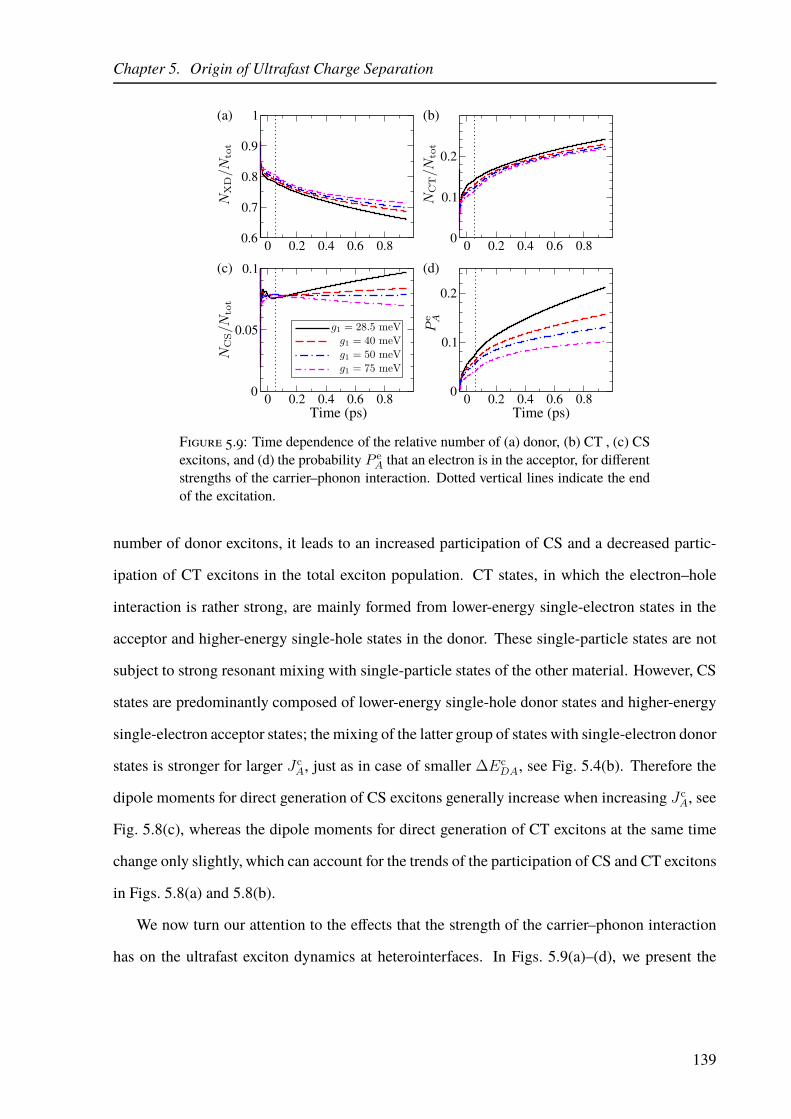
Chapter 5. Origin of Ultrafast Charge Separation
Time (ps) Time (ps)
0 0.2 0.4 0.6 0.80.6
0.7
0.8
0.9
1
0 0.2 0.4 0.6 0.80
0.1
0.2
0 0.2 0.4 0.6 0.80
0.05
0.1
0 0.2 0.4 0.6 0.80
0.1
0.2
(a) (b)
(c) (d)
Figure 5.9: Time dependence of the relative number of (a) donor, (b) CT , (c) CSexcitons, and (d) the probability P e
A that an electron is in the acceptor, for differentstrengths of the carrier–phonon interaction. Dotted vertical lines indicate the endof the excitation.
number of donor excitons, it leads to an increased participation of CS and a decreased partic-
ipation of CT excitons in the total exciton population. CT states, in which the electron–hole
interaction is rather strong, are mainly formed from lower-energy single-electron states in the
acceptor and higher-energy single-hole states in the donor. These single-particle states are not
subject to strong resonant mixing with single-particle states of the other material. However, CS
states are predominantly composed of lower-energy single-hole donor states and higher-energy
single-electron acceptor states; the mixing of the latter group of states with single-electron donor
states is stronger for larger JcA, just as in case of smaller ∆Ec
DA, see Fig. 5.4(b). Therefore the
dipole moments for direct generation of CS excitons generally increase when increasing JcA, see
Fig. 5.8(c), whereas the dipole moments for direct generation of CT excitons at the same time
change only slightly, which can account for the trends of the participation of CS and CT excitons
in Figs. 5.8(a) and 5.8(b).
We now turn our attention to the effects that the strength of the carrier–phonon interaction
has on the ultrafast exciton dynamics at heterointerfaces. In Figs. 5.9(a)–(d), we present the
139
Chapter 5. Origin of Ultrafast Charge Separation
results with the fixed ratio g2/g1 = 2.0 and the polaron binding energies defined in Eq. (5.8) as-
suming the values of approximately 20, 40, 60, and 140 meV, in ascending order of g1. We note
that it is not straightforward to predict the effect of the variations of carrier–phonon interaction
strength on the population of space-separated states. Single-phonon-assisted processes prefer-
entially couple exciton states of the same character, i.e., a donor exciton state is more strongly
coupled to another donor state than to a space-separated state. This is apparent from Eq. (5.7)
that expresses the carrier–phonon matrix elements in the exciton basis. On the one hand, stronger
carrier–phonon interaction implies more pronounced exciton dissociation and charge separation
because of stronger coupling between donor and space-separated states. On the other hand,
stronger carrier–phonon interaction leads to faster relaxation of initially generated donor exci-
tons within the donor exciton manifold to low-lying donor states. Low-lying donor states are
essentially uncoupled from space-separated states, i.e., they exhibit low probabilities of exciton
dissociation and charge separation. Our results, shown in Figs. 5.9(a)–(d), indicate that stronger
carrier–phonon interaction leads to smaller number of CT and CS excitons, as well as the prob-
ability that an electron is in the acceptor, and to greater number of donor excitons. We also note
that stronger carrier–phonon interaction changes the trend displayed by the population of CS
states. While for the weakest interaction studied CS population grows after the excitation, for
the strongest interaction studied CS population decays after the excitation. This is a consequence
of more pronounced phonon-assisted processes leading to population of low-energy CT states
once a donor exciton performs a transition to a space-separated state. This discussion can ratio-
nalize the changes in relevant quantities summarized in Figs. 5.9(a)–(d); the magnitudes of the
changes observed are, however, rather small. In previous studies [141, 142], which did not deal
with the initial exciton generation step, stronger carrier–phonon interaction is found to suppress
quite strongly the charge separation process. The weak influence of the carrier–phonon interac-
tion strength on ultrafast heterojunction dynamics that we observe supports the mechanism of
ultrafast direct optical generation of space-separated charges. If the charge separation process at
heterointerfaces were mainly driven by the free-system evolution, greater changes in the quan-
tities describing charge separation efficiency would be expected with varying carrier–phonon
interaction strength.
140

Chapter 5. Origin of Ultrafast Charge Separation
Time (ps)
Electron position
0 0.2 0.4 0.6 0.80.5
0.6
0.7
0.8
0.9
1
0 0.2 0.4 0.6 0.80
0.1
0.2
0 0.2 0.4 0.6 0.80
0.1
0.2
0 5 10 15 200
0.05
0.1
(a) (b)
(c) (d)
Time (ps)
Figure 5.10: Time dependence of the relative number of: (a) donor, (b) CT, and (c)CS excitons for different ratios g2/g1 of high-frequency to low-frequency phononmode coupling constants. (d) The distribution of an electron throughout the systemfe(t, r) 900 fs after the end of the pulsed excitation for different ratios g2/g1.
Additionally, we perform computations for a fixed value of ǫpolb = 20 meV and different
values of the ratio g2/g1 among coupling constants of high- and low-frequency phonon modes.
The result presented in Fig. 5.10(a)–(d) shows that the increase of the ratio g2/g1 increases the
number of CT excitons and decreases the number of donor excitons, while the population of
CS states exhibits only a weak increase. Stronger coupling to the high-frequency phonon mode
(with respect to the low-frequency one) enhances charge separation by decreasing the number of
donor excitons, but at the same time promotes phonon-assisted processes towards more strongly
bound CT states, which is seen in Fig. 5.10(d) as larger probability fe on acceptor sites close to
the interface (sites 11–14). Consequently, the population of CS states remains nearly constant.
In the end, let us comment on the influence of temperature on the ultrafast exciton dynamics
at a heterojunction. Results presented in Figs. 5.11(a)–(d) suggest that the ultrafast dynamics
exhibits weak temperature dependence, which is consistent with existing theoretical [152] and
experimental [153] insights, and also with the mechanism of direct optical generation of space-
separated carriers. However, we observe that at lower temperature the normalized number of
141

Chapter 5. Origin of Ultrafast Charge Separation
0 0.2 0.4 0.6 0.80
0.2
0.4
0.6
0.8
1
0 5 10 15 200
0.05
0.1
0 0.2 0.4 0.6 0.80
0.2
0.4
0.6
0.8
1
0 0.2 0.4 0.6 0.80
0.2
0.4
0.6
0.8
1(a) (b)
(c) (d)
Time (ps)
Time (ps)
Electron position
Figure 5.11: Time dependence of the relative number of: (a) donor, (b) CT, and (c)CS excitons for different temperatures. (d) The distribution of an electron through-out the system fe(t, r) 900 fs after the end of the pulsed excitation for differenttemperatures.
donor excitons slightly decreases, while normalized numbers of CT and CS excitons weakly in-
crease. Additionally, we observe an increase in the probability that an electron is located in the
acceptor next to the interface (sites 11–14) as the temperature is decreased, which is a manifes-
tation of larger population of bound (low-energy) CT states as the temperature is decreased.
In summary, we find that regardless of the particular values of varied model parameters
(Jc/vDA,∆E
cDA, J
cA, carrier–phonon coupling constants), the majority of CT and CS states that
are present at ∼ 100 fs after photoexcitation have been directly generated during the excitation.
Trends in quantities describing ultrafast heterojunction dynamics that we observe varying model
parameters can be explained by taking into consideration the proposed mechanism of ultrafast
direct optical generation of space-separated charges.
5.4 Ultrafast Spectroscopy Signatures
As discussed in Sec. 5.1.1, exciton dynamics on ultrafast time scales is typically probed ex-
perimentally using the ultrafast pump–probe spectroscopy. In such experiments, the presence
142

Chapter 5. Origin of Ultrafast Charge Separation
of space-separated charges on ultrafast time scales after photoexcitation has been established
and the energy resonance between donor exciton and space-separated states was identified as re-
sponsible for efficient charge generation [36], in agreement with our numerical results. However,
while our results indicate that the majority of space-separated charges that are present at ∼ 100
fs after photoexcitation have been directly optically generated, interpretation of experiments [36]
suggests that these states become populated by the transition from donor exciton states. To un-
derstand the origin of this apparent difference, we numerically compute ultrafast pump–probe
signals in the framework of our heterojunction model. For completeness, Sec. 5.4.1 briefly sum-
marizes the conventional interpretation of experimental DTSs, which focuses on the dynamics
of populations and completely disregards coherences. In Sec. 5.4.2, we present the theoretical
treatment of ultrafast TA experiments adapted for the system at hand. Assuming that the probe
pulse is deltalike, we obtain an analytic expression relating the differential transmission ∆T to
the nonequilibrium state of the system “seen” by the probe pulse. The expression provides a
very clear and direct interpretation of the results of ultrafast TA experiments and allows to dis-
tinguish between contributions stemming from exciton populations and coherences, challenging
the existing interpretations. It is used in Sec. 5.4.3 to numerically compute DTSs.
5.4.1 Basics of Ultrafast Transient Absorption Spectroscopy and Conven-
tional Interpretation of Experimental Signals
Figure 5.12(a) depicts the principle scheme of a femtosecond time-resolved TA spectroscopy
experiment [154–156]. The sample is first irradiated by an intense pump pulse that excites the
sample and initiates the nonequilibrium dynamics of the excited species. Temporal evolution of
the state of the sample is subsequently examined using a second, weaker, probe pulse, whose
time delay with respect to the pump pulse (the so-called pump–probe delay τ ) can be tuned.
Pulse duration limits the temporal resolution of the experiment, so that pulses should be as short
as possible to resolve the fastest photophysical processes. On the other hand, the pump pulse
should be as spectrally narrow as possible, so that it can selectively excite the optical transi-
tion of interest. Therefore, there is a trade-off between the temporal and spectral resolution in a
143

Chapter 5. Origin of Ultrafast Charge Separation
transmitted probewith pump
transmitted probewithout pump
(a) (b)
Figure 5.12: (a) Schematic view of a femtosecond time-resolved TA experiment.The pump is essentially monochromatic, whereas the probe is a broadband pulse.(b) Calculation of the DTS. Adapted from Ref. [156] with permission of The RoyalSociety of Chemistry (RSC) on behalf of the Centre National de la RechercheScientifique (CNRS) and the RSC.
pump–probe experiment. The probe pulse should be as short as possible, because a spectrally
wide (broadband) probe pulse enables simultaneous measurements at many different frequen-
cies. Having passed through the sample, the broadband probe pulse is spectrally resolved in a
spectrometer. The experimental quantity of interest is the DTS that is a function of both the
probe frequency ωpr and the pump–probe delay τ
∆T
T(τ ;ωpr) =
T neq (τ ;ωpr)− T eq (ωpr)
T eq (ωpr). (5.19)
The transmission of the sample that is initially (before the action of the probe) unexcited is
denoted by T eq (ωpr) and it is an equilibrium property of the sample. On the other hand, the
transmission of the pump-driven systemT neq (τ ;ωpr) is a nonequilibrium quantity and it depends
on both the probe frequency and the time delay between the pump and probe.
The conventional interpretation of the DTS is performed by disregarding coherent effects
and concentrating on the dynamics of populations of excited states [155, 156]. The action of
the pump pulse populates excited states by reducing the occupation of the ground state. Let us
distinguish between different types of the DTS.
(a) If the probe frequency is greater than or equal to the ground state absorption edge, the
absorption of the pumped sample is weaker than the equilibrium absorption, because the
144
Chapter 5. Origin of Ultrafast Charge Separation
ground state population is depleted by pumping. In other words, the transmission of the
pumped sample is greater than the equilibrium transmission, and the DTS is positive. Such
a signal is commonly denoted as the ground state bleaching (GSB).
(b) If the probe frequency is less than or equal to the ground state absorption edge, a probe
photon may trigger the stimulated emission from the excited state back to the ground state.
The stimulated emission (SE) is characterized by a positive DTS.
(c) The probe frequency may be resonant with a transition from an excited state to some other
higher-lying excited state. The hallmark of the photoinduced absorption (PIA) is a negative
DTS. In principle, PIA signal can be observed at any probe frequency, depending on the
energy levels of the system under study.
Let us now emphasize that an analysis of an experimental DTS and its deconvolution into
the above-mentioned three types of signals is a highly nontrivial task. For example, since PIA
may occur at any probe frequency, it may spectrally overlap with GSB and SE signals, and
even prevail over them. The interpretation of experimental signals, therefore, is usually done in
combination with the results of quantum chemical calculations, from which one can gain insight
into the excitation energies of the system, as well as possible transitions between excited states.
5.4.2 Theoretical Treatment of Ultrafast Transient Absorption Spectroscopy
Our theoretical approach to a TA experiment considers the interaction with the pump pulse as
described in Ch. 3, i.e., within the density matrix formalism employing the DCT scheme up to
the second order in the pump field. Furthermore, we assume that the interaction with the probe
pulse does not change significantly the nonequilibrium state created by the pump pulse, and it is
treated in the linear response regime. The corresponding nonequilibrium dipole–dipole retarded
correlation function is then used to calculate DTSs [157, 158].
To study time-resolved TA experiments, we extend our two-band lattice model of a bilayer by
including more single-electron (single-hole) energy levels per site. More details on this multi-
band model can be found in Sec. 6.2, where its Hamiltonian is precisely formulated. Here,
145

Chapter 5. Origin of Ultrafast Charge Separation
we investigate in more details only those aspects of the multiband model that are necessary to
formulate a theoretical framework in which ultrafast TA experiments can be studied. Multiple
single-electron (single-hole) levels on each site should be dipole-coupled among themselves in
order to enable probe-induced transitions between various exciton states. We denote by c†iβi
(ciβi) creation (annihilation) operators for electrons on site i and in conduction-band orbital βi;
similarly, d†iαi(diαi
) create (annihilate) a hole on site i and in valence-band orbital αi. The
dipole-moment operator in terms of electron and hole operators assumes the form
P =∑
iβiαi
dcvi
(
c†iβid†iαi
+ diαiciβi
)
+∑
iβi 6=β′
i
dcci c†iβiciβ′
i−∑
iαi 6=α′
i
dvvi d†iα′
idiαi
. (5.20)
Intraband dipole matrix elements dcci (dvvi ) describe electron (hole) transitions between differ-
ent single-electron (single-hole) states on site i, as opposed to the interband matrix elements
dcvi , which are responsible for the exciton generation. Performing transition to the exciton ba-
sis, which is defined analogously to Eq. (5.5) [see also Eq. (6.4)], dipole matrix elements for
transitions from the ground state to exciton state x are [see also Eq. (6.5)]
Mx =∑
iβiαi
dcvi ψx∗(iαi)(iβi)
, (5.21)
while those for transitions from exciton state x to exciton state x are
Mxx =
∑
iαi 6=α′
i
∑
jβj
ψx∗(iαi)(jβj)
dvvi ψx(iα′
i)(jβj)−∑
iβi 6=β′
i
∑
jαj
ψx∗(jαj)(iβ′
i)dcci ψ
x(jαj)(iβi)
. (5.22)
Further developments are facilitated by working with the Hamiltonian that is explicitly expressed
in terms of exciton creation and annihilation operators, see Eq. (3.89), and that is relevant for
the second-order (low-density) dynamics. The operator P [Eq. (5.20)] expressed in terms of
operators Xx, X†x, which are defined as
X†x =
∑
iαijβj
ψx(iαi)(jβj)
c†jβjd†iαi
, (5.23)
146

Chapter 5. Origin of Ultrafast Charge Separation
assumes the form
P =∑
x
(MxX
†x +M∗
xXx
)−∑
xx
MxxX
†xXx. (5.24)
In the last equation, we retain only contributions whose expectation values are at most of the
second order in the pump field.
We concentrate on the so-called nonoverlapping regime [157], in which the probe pulse,
described by its electric field e(t), acts after the pump pulse. We take that our system meets
the condition of optical thinness, i.e., the electromagnetic field originating from probe-induced
dipole moment can be neglected compared to the electromagnetic field of the probe. In the
following considerations, the origin of time axis t = 0 is taken to be the instant at which the
probe pulse starts. The pump pulse finishes at t = −τ , where τ is the time delay between (the
end of) the pump and (the start of) the probe. The pump creates a nonequilibrium state of the
system which is, at the moment when the probe pulse starts, described by the density matrix
ρ(0), which implicitly depends on the pump–probe delay τ .
In the linear-response regime, the probe-induced dipole moment dp(t) for t > 0 is expressed
as [157]
dp(t) =
∫
dt′ χ(t, t′) e(t′), (5.25)
where χ(t, t′) is the nonequilibrium retarded dipole–dipole correlation function
χ(t, t′) = − i
~θ(t− t′)Tr (ρ(0)[P (t), P (t′)]) . (5.26)
Time dependence in Eq. (5.26) is governed by the Hamiltonian of the system in the absence of
external fields [Eq. (3.89)]
HE(t)=0 = H0 +Hx−p, (5.27)
where H0 is the noninteracting Hamiltonian of excitons in the phonon field [the first two terms
on the right-hand side of Eq. (3.89)], while Hx−p accounts for exciton–phonon interaction [the
third term on the right-hand side of Eq. (3.89)]. For an ultrashort probe pulse, e(t) = e0δ(t),
147

Chapter 5. Origin of Ultrafast Charge Separation
probe-induced dipole moment assumes the form
dp(t) = e0χ(t, 0) = e0
(
− i
~
)
Tr (ρ(0)[P (t), P (0)]) . (5.28)
The probe pulse tests the possibility of transitions between various exciton states, i.e., it primar-
ily affects carriers. Therefore, as a reasonable approximation to the full time-dependent operator
P (t) appearing in Eq. (5.28), operator P (0)(t), evolving according to the noninteracting Hamil-
tonian H0 in Eq. (5.27), may be used. This leads us to the central result for the probe-induced
dipole moment:
dp(t) = e0
(
− i
~
)
Tr(ρ(0)[P (0)(t), P (0)]
). (5.29)
The commutator on the right-hand side of Eq. (5.29) can be derived using the commutation
relations embodied in Eq. (3.87), in which four-index coefficients C x′x′
xx defined in Eq. (3.88)
assume the form
C x′x′
xx =∑
jβj
jβj
(∑
iαi
ψx′∗(iαi)(j βj)
ψx′
(iαi)(jβj)
)(∑
iαi
ψx(iαi)(j βj)
ψx∗(iαi)(jβj)
)
+∑
iαiiαi
∑
jβj
ψx′∗(iαi)(jβj)
ψx′
(iαi)(jβj)
∑
jβj
ψx(iαi)(jβj)
ψx∗(iαi)(jβj)
.
(5.30)
The final result for the commutator [P (0)(t), P (0)] is
[P (0)(t), P (0)] =∑
x
|Mx|2(e−iωxt − eiωxt
)
−∑
x1x1
∑
xx′
(M∗
xMx′C x1x1
x′x e−iωxt −MxM∗x′C x1x1
xx′ eiωxt)X†
x1Xx1
−∑
xx′
(MxMxx′)
∗ e−iωxtXx′ +∑
xx′
MxMxx′eiωxtX†
x′
+∑
xx′
(MxMxx′)
∗ e−i(ωx′−ωx)tXx′ −∑
xx′
MxMxx′ei(ωx′−ωx)tX†
x′
+∑
xxx′
Mxx′M x
x ei(ωx′−ωx)tX†
x′Xx −∑
xxx′
Mx′
x Mxx e
−i(ωx′−ωx)tX†xXx′ .
(5.31)
The expectation values [with respect to ρ(0)] of the operators appearing in the last equation are
148

Chapter 5. Origin of Ultrafast Charge Separation
simply the active purely electronic density matrices of our formalism computed when the probe
pulse starts, i.e., Tr (ρ(0)Xx) = yx(0) and Tr(
ρ(0)X†xXx
)
= nxx(0).
Inserting Eq. (5.31) into Eq. (5.29), we observe two different types of contributions to the
probe-induced dipole moment dp(t). Contributions of the first type oscillate at frequencies ωx
corresponding to probe-induced transitions between the ground state and exciton state x, while
those of the second type oscillate at frequencies ωx − ωx corresponding to probe-induced tran-
sitions between exciton states x and x. Here, we focus our attention on the process of PIA, in
which an exciton in state x performs a transition to another state x under the influence of the
probe field. Therefore, we will further consider only the second type of contributions, i.e., in
the expression for the commutator [P (0)(t), P (0)], we retain only the last four summands on the
right-hand side of Eq. (5.31).
The frequency-dependent transmission coefficient T (ω) is defined as [157] (we use SI units)
T (ω) = 1 +cµ0
S~ Im
~ωdp(ω)
e(ω)
, (5.32)
where dp(ω) and e(ω) are Fourier transformations of dp(t) and e(t), respectively, S is the ir-
radiated area of the sample, while µ0 is the magnetic permeability of the vacuum. Here, we
concentrate on obtaining an expression for part of the differential transmission that stems from
processes of PIA. In Eq. (5.19), the equilibrium transmission of the sample T eq(ω) appears.
However, T eq(ω) is expected to reflect only transitions involving the ground state, because it is a
property of the unexcited sample. Since our aim is to make only qualitative, but not quantitative,
comparisons to experimental PIA signals, we will not further consider T eq(ω). We compute
∆TPIA (τ ;ω) = T neqPIA (τ ;ω) , (5.33)
where T neqPIA (τ ;ω) is computed by the Fourier transformation of the aforementioned second type
149

Chapter 5. Origin of Ultrafast Charge Separation
of contributions to the probe-induced dipole moment dp(t). Computing the Fourier transforma-
tion dp(ω), we obtain integrals of the type
∫ +∞
0
dt ei(ω−Ω+iη)t =i
ω − Ω+ iη, (5.34)
where we have introduced a positive infinitesimal parameter η to ensure the integral convergence.
Physically, introducing η effectively accounts for the line broadening [158]. For simplicity, we
assume that only one value of η is used in all the integrals of the type (5.34). Finally, inserting
the result for dp(ω) into Eqs. (5.32) and (5.33), the following expression is obtained
∆TPIA(τ ;ω) ∝ Im
∑
xx′
(MxMxx′)∗
~ω
~ω − (~ωx′ − ~ωx) + iηyx′(0) −
−∑
xx′
MxMxx′
~ω
~ω + (~ωx′ − ~ωx) + iηy∗x′(0) +
+∑
xxx′
Mxx′M x
x
~ω
~ω + (~ωx′ − ~ωx) + iηy∗x′(0)yx(0) −
−∑
xxx′
Mx′
x Mxx
~ω
~ω − (~ωx′ − ~ωx) + iηy∗x(0)yx′(0) +
+∑
xxx′
Mxx′M x
x
~ω
~ω + (~ωx′ − ~ωx) + iηnx′x(0) −
−∑
xxx′
Mx′
x Mxx
~ω
~ω − (~ωx′ − ~ωx) + iηnxx′(0)
.
(5.35)
In the last equation, we have explicitly separated coherent from incoherent contributions by intro-
ducing the correlated parts of exciton populations and exciton–exciton coherences nxx, whose
definition is given in Eq. (3.47). The coherences between exciton states and the ground state
yx(0), as well as correlated parts of exciton–exciton coherences nxx(0) (x 6= x), are expected to
approach zero for sufficiently long time delays between the pump and the probe. In this limit,
Eq. (5.35) contains only incoherent exciton populations nxx:
∆TPIA(τ ;ω) ∝−∑
xx′
|Mxx′|2 η · ~ω
(~ω + (~ωx′ − ~ωx))2 + η2nx′x′(0)
+∑
xx′
|Mxx′|2 η · ~ω
(~ω − (~ωx′ − ~ωx))2 + η2nx′x′(0).
(5.36)
150

Chapter 5. Origin of Ultrafast Charge Separation
This expression is manifestly negative when it describes probe-induced transitions from exci-
ton state x′ to some higher-energy exciton state x. The last conclusion is in agreement with the
usual experimental interpretation of pump–probe spectra, where negative DTS corresponds to
PIA [155]. It is expected that Eq. (5.36) correctly describes the PIA signal on picosecond or
longer time scales, because the coherences between exciton states and the ground state yx typ-
ically decay on . 100-fs time scale after the pump field has vanished, while exciton–exciton
coherences typically decay on picosecond time scales or longer. Our full expression for the
PIA signal [Eq. (5.35)] demonstrates that, in the ultrafast regime, it is expected that both coher-
ences between exciton states and the ground state yx(0) and exciton–exciton coherences nxx(0)
(x 6= x), along with incoherent exciton populations nxx(0), play significant role. The signal
embodied Eq. (5.35) describes PIA, but it is not manifestly negative. Therefore, our theoretical
developments suggest that the correspondence between the sign of the differential transmission
signal and its type (GSB, SE, or PIA) does not necessarily hold on ultrafast time scales.
5.4.3 Numerical Results: Ultrafast Differential Transmission Signals
In order to compute PIA signals and at the same time keep the numerics manageable, we ex-
tend our model by introducing only one additional single-electron level both in the donor and in
the acceptor and one additional single-hole level in the donor. Such an extension is motivated
by the fact that the dipole-induced coupling between two exciton states is strongest when these
two states are of the same character, see Eqs. (5.22) and (5.24). Therefore, probing the PIA
from donor (space-separated) states is expected to involve higher-lying donor (space-separated)
states, the existence of which requires additional higher-lying single-electron states in both ma-
terials and higher-lying single-hole states in the donor. Additional energy levels in the donor and
the corresponding bandwidths are extracted from the aforementioned electronic structure calcu-
lation on an infinitely long PCPDTBT polymer chain. The additional single-electron level is
located ca. 1.16 eV above the single-electron level used in all the calculations and the bandwidth
of the corresponding zone is estimated to be ca. 0.48 eV. The additional single-hole level is lo-
cated ca. 1.13 eV below the single-hole level used in all the calculations and the bandwidth of the
151

Chapter 5. Origin of Ultrafast Charge Separation
corresponding zone is estimated to be ca. 0.57 eV. The additional energy level in the acceptor is
extracted from an electronic structure calculation on the C60 molecule. The calculation is based
on DFT using either LDA or B3LYP exchange–correlation functional (both choices give similar
results) and 6-31G basis set and was performed using the NWChem package [159]. We found
that the additional single-electron level lies around 1 eV above the single-electron level used in
all the calculations. The bandwidth of the corresponding zone is set to 0.6 eV, see Table 5.1.
Here, we assume that the waveform of the pump pulse is
E(t) = E0 cos(ωct) exp
(
− t2
τ 2G
)
θ(t + t0)θ(t0 − t), (5.37)
where we take τG = 20 fs and t0 = 50 fs, while the probe is
e(t) = e0δ(t− (t0 + τ)), (5.38)
with variable pump–probe delay τ . The intraband dipole matrix elements dcci , dvvi in Eq. (5.20)
are assumed to be equal in the whole system
dcci = dvvi = dintra =1
2dcv. (5.39)
The positive parameter η, which effectively accounts for the line broadening, is set to η = 50 meV.
Variations in η do not change qualitative features of the presented PIA spectra, which was
checked in the Supplementary Material associated to Ref. [134]. In actual computations of the
signal given in Eq. (5.35), we should remember that the pump pulse finishes at instant t0, while in
Eq. (5.35) all the quantities are taken at the moment when the probe starts, which is now t0+τ ; in
other words, yx(0) → yx(t0+ τ), nxx(0) → nxx(t0+ τ) when we compute pump–probe signals
using Eq. (5.35) and the pump and probe are given by Eqs. (5.37) and (5.38), respectively.
In the following, we separately show the total signal [full Eq. (5.35)], the y-part of the signal
[the first two sums in Eq. (5.35)], and the n-part of the signal [the third sum in Eq. (5.35)]. We
note that it would be possible to further separate the n-part of the signal into the contribution
stemming from incoherent exciton populations nxx [Eq. (5.36)] and exciton–exciton coherences
152
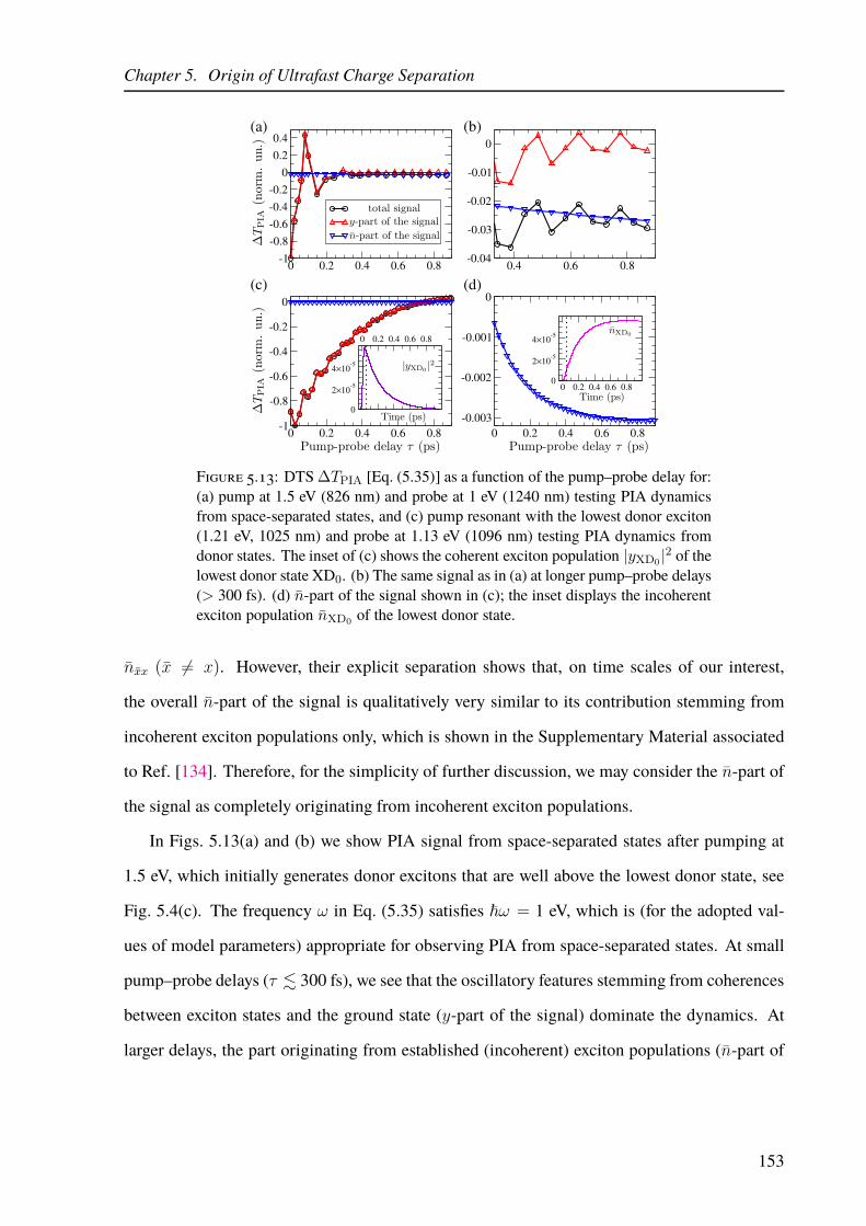
Chapter 5. Origin of Ultrafast Charge Separation
(a) (b)
(c) (d)
0 0.2 0.4 0.6 0.8-1
-0.8
-0.6
-0.4
-0.2
0
0.2
0.4
0.4 0.6 0.8-0.04
-0.03
-0.02
-0.01
0
0 0.2 0.4 0.6 0.8-1
-0.8
-0.6
-0.4
-0.2
0
0 0.2 0.4 0.6 0.8
-0.003
-0.002
-0.001
0
0 0.2 0.4 0.6 0.80
2×10⁻⁵
4×10⁻⁵
0 0.2 0.4 0.6 0.8
0
2×10⁻⁵
4×10⁻⁵
Figure 5.13: DTS ∆TPIA [Eq. (5.35)] as a function of the pump–probe delay for:(a) pump at 1.5 eV (826 nm) and probe at 1 eV (1240 nm) testing PIA dynamicsfrom space-separated states, and (c) pump resonant with the lowest donor exciton(1.21 eV, 1025 nm) and probe at 1.13 eV (1096 nm) testing PIA dynamics fromdonor states. The inset of (c) shows the coherent exciton population |yXD0 |2 of thelowest donor state XD0. (b) The same signal as in (a) at longer pump–probe delays(> 300 fs). (d) n-part of the signal shown in (c); the inset displays the incoherentexciton population nXD0 of the lowest donor state.
nxx (x 6= x). However, their explicit separation shows that, on time scales of our interest,
the overall n-part of the signal is qualitatively very similar to its contribution stemming from
incoherent exciton populations only, which is shown in the Supplementary Material associated
to Ref. [134]. Therefore, for the simplicity of further discussion, we may consider the n-part of
the signal as completely originating from incoherent exciton populations.
In Figs. 5.13(a) and (b) we show PIA signal from space-separated states after pumping at
1.5 eV, which initially generates donor excitons that are well above the lowest donor state, see
Fig. 5.4(c). The frequency ω in Eq. (5.35) satisfies ~ω = 1 eV, which is (for the adopted val-
ues of model parameters) appropriate for observing PIA from space-separated states. At small
pump–probe delays (τ . 300 fs), we see that the oscillatory features stemming from coherences
between exciton states and the ground state (y-part of the signal) dominate the dynamics. At
larger delays, the part originating from established (incoherent) exciton populations (n-part of
153

Chapter 5. Origin of Ultrafast Charge Separation
the signal) prevails, see Fig. 5.13(b), and the shape of the signal resembles the shapes of sig-
nals from space-separated states in Fig. 4(c) of Ref. [36]. The signal decreases at larger delays,
which correlates very well with the fact that the numbers of CT and CS excitons increase, see
Fig. 5.5(a). In other words, at larger pump–probe delays, at which the influence of coherences
between exciton states and the ground state is small, the signal can be unambiguously interpreted
in terms of charge transfer from the donor to the acceptor.
Figures 5.13(c) and (d) display PIA signal from donor excitons following the pump excitation
at the lowest donor state (1.21 eV). The frequency ω in Eq. (5.35) satisfies ~ω = 1.13 eV, which
is appropriate for studying the PIA from donor states. The overall signal shape is qualitatively
similar to the shape of donor exciton PIA signal in Fig. 4(a) of Ref. [36], but the interpretation
of its origin is rather different. While the authors of Ref. [36] suggest that the monotonically
increasing PIA signal from donor excitons reflects their transfer to space-separated states, our
signal predominantly originates from coherences between donor states and the ground state [y-
part of the signal in Fig. 5.13(c)]. Furthermore, the shape of the total signal matches very well
the decay of the coherent population of the lowest donor exciton, see the inset of Fig. 5.13(c),
while the shape of the n-part of the signal corresponds well to the changes in the incoherent
population of the lowest donor state, see the inset of Fig. 5.13(d). This incoherent population
does not decay during our computation: immediately after the pump pulse it rises and at longer
times it reaches a plateau, which signals that the donor exciton population is "blocked" in the
lowest donor state. The lowest donor exciton is very strongly dipole-coupled to the ground state,
its population comprising around 75% of the total generated population. Therefore, according to
our numerical results, the observed PIA signal from donor excitons in this case mimics the con-
version from coherent to incoherent exciton population of the lowest donor state. This, however,
does not necessarily mean that the concomitant charge transfer is completely absent in this case.
Instead, the presence of coherences between exciton states and the ground state, which domi-
nate the signal for all pump–probe delays we studied, prevents us from attributing the signal to
the population transfer from donor excitons to space-separated states. The aforementioned con-
version from coherent to incoherent exciton population of the lowest donor state is rather slow
because of the relatively weak coupling between low-lying donor excitons on the one hand and
154

Chapter 5. Origin of Ultrafast Charge Separation
space-separated states on the other hand (this weak coupling was also appreciated in Ref. [36]).
On the other hand, pumping well above the lowest donor and space-separated states, the cou-
plings between these species are stronger and more diverse than for the pump resonant with the
lowest donor exciton; this situation resembles the one encountered for the excitation condition
in Fig. 4(c) of Ref. [36].
5.5 Discussion and Significance of Our Results
In this chapter, we have presented a study of the subpicosecond exciton dynamics in a one-
dimensional model of a D/A heterointerface. The principal advantage of our method over other
methods used in literature [52, 58, 141, 142, 160] is the fact that it treats both the generation
of excitons and their further separation on equal footing and that it deals with all the relevant
interactions on a fully quantum level. Since we explicitly consider the exciton generation from
an initially unexcited heterojunction, we are able to assess the importance of the direct optical
generation of spatially separated charges with respect to other proposed mechanisms of their
generation on subpicosecond time scales. We find that the resonant electronic coupling between
donor and space-separated states does not only enhance the transfer from the former to the latter
group of states [36, 49], but also opens up a new and important pathway to obtain space-separated
charges: their direct optical generation [143, 144]. While this mechanism has been proposed on
the basis of electronic structure and model Hamiltonian calculations, which did not include any
dynamics, our study is, to the best of our knowledge, the first to investigate the possibility of
direct optical generation of separated charges by performing a fully quantum and statistical in-
vestigation of ultrafast exciton dynamics at a heterointerface. We conclude that the largest part of
space-separated charges that are present on ∼ 100-fs time scales after the initial photoexcitation
are directly optically generated, contrary to the general belief that they originate from ultrafast
transitions from donor states. Our results, therefore, do not only confirm the theoretical hypothe-
ses about the possibility of the direct optical generation of space-separated charges [143, 144],
but position them into a wider framework by performing a study of subpicosecond dynamics of
electronic excitations in a photoexcited D/A blend.
155

Chapter 5. Origin of Ultrafast Charge Separation
The resonant coupling between states of donor excitons and space-separated charges is at
the heart of the direct optical generation of the latter group of states. This coupling is mediated
by the D/A transfer integrals (JcDA, J
vDA) and it ultimately originates from the resonant mixing
between single-electron states in the donor and acceptor parts of the heterojunction. It makes
space-separated states acquire nonzero dipole moment from states of donor excitons. In other
words, it is a redistribution of oscillator strengths between donor and space-separated states that
makes the latter group of states accessible directly from the ground state. The last point was
previously highlighted in studies conducted on two- [143] and three-dimensional [144] hetero-
junction models. Differently from our one-dimensional model, in which the D/A coupling is
restricted to only two sites (N − 1 and N) adjacent to the interface, in higher-dimensional mod-
els the dominant part of the D/A coupling involves more than a single pair of sites. Since we
convincingly demonstrate that, in our one-dimensional model, the redistribution of oscillator
strengths promotes the direct optical generation into the main source of space-separated carriers
on ultrafast time scales, we speculate that this conclusion would remain valid in a more realis-
tic higher-dimensional model of a heterointerface. While there is absorption intensity transfer
from donor to space-separated states brought about by their resonant mixing, the absorption still
primarily occurs in the donor part of a heterojunction, see Fig. 5.5(a). Our results show that on
ultrafast time scales the direct optical generation as a source of space-separated carriers is more
important than transitions from donor to space-separated states. This, however, does not mean
that initially generated donor excitons are not transformed into space-separated states. They
indeed are, see Figs. 5.5(a) and (b), but the characteristic time scale on which populations of
space-separated states change due to the free-system evolution is longer than 100 fs.
We find that regardless of the particular values of varied model parameters (Jc/vDA,∆E
cDA, J
cA,
carrier–phonon coupling constants), the majority of CT and CS states that are present at∼ 100 fs
after photoexcitation have been directly generated during the excitation. The ultrafast generation
of separated charges at heterointerfaces is more pronounced when the D/A electronic coupling
(JcDA, J
vDA) is larger or when the energy overlap region between single-electron states in the
donor and acceptor is wider, either by increasing the electronic coupling JcA in the acceptor
or decreasing the LUMO–LUMO offset ∆EcDA between the two materials, see Fig. 5.4(b). Our
156
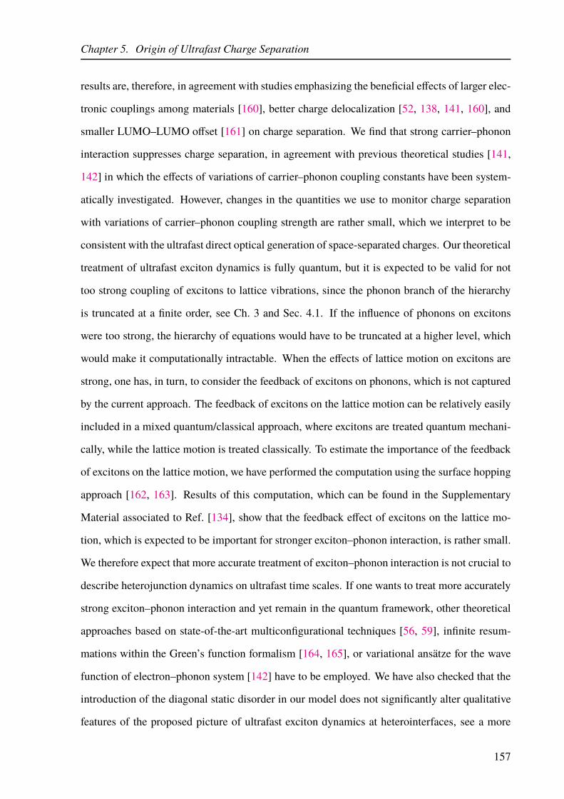
Chapter 5. Origin of Ultrafast Charge Separation
results are, therefore, in agreement with studies emphasizing the beneficial effects of larger elec-
tronic couplings among materials [160], better charge delocalization [52, 138, 141, 160], and
smaller LUMO–LUMO offset [161] on charge separation. We find that strong carrier–phonon
interaction suppresses charge separation, in agreement with previous theoretical studies [141,
142] in which the effects of variations of carrier–phonon coupling constants have been system-
atically investigated. However, changes in the quantities we use to monitor charge separation
with variations of carrier–phonon coupling strength are rather small, which we interpret to be
consistent with the ultrafast direct optical generation of space-separated charges. Our theoretical
treatment of ultrafast exciton dynamics is fully quantum, but it is expected to be valid for not
too strong coupling of excitons to lattice vibrations, since the phonon branch of the hierarchy
is truncated at a finite order, see Ch. 3 and Sec. 4.1. If the influence of phonons on excitons
were too strong, the hierarchy of equations would have to be truncated at a higher level, which
would make it computationally intractable. When the effects of lattice motion on excitons are
strong, one has, in turn, to consider the feedback of excitons on phonons, which is not captured
by the current approach. The feedback of excitons on the lattice motion can be relatively easily
included in a mixed quantum/classical approach, where excitons are treated quantum mechani-
cally, while the lattice motion is treated classically. To estimate the importance of the feedback
of excitons on the lattice motion, we have performed the computation using the surface hopping
approach [162, 163]. Results of this computation, which can be found in the Supplementary
Material associated to Ref. [134], show that the feedback effect of excitons on the lattice mo-
tion, which is expected to be important for stronger exciton–phonon interaction, is rather small.
We therefore expect that more accurate treatment of exciton–phonon interaction is not crucial to
describe heterojunction dynamics on ultrafast time scales. If one wants to treat more accurately
strong exciton–phonon interaction and yet remain in the quantum framework, other theoretical
approaches based on state-of-the-art multiconfigurational techniques [56, 59], infinite resum-
mations within the Green’s function formalism [164, 165], or variational ansätze for the wave
function of electron–phonon system [142] have to be employed. We have also checked that the
introduction of the diagonal static disorder in our model does not significantly alter qualitative
features of the proposed picture of ultrafast exciton dynamics at heterointerfaces, see a more
157

Chapter 5. Origin of Ultrafast Charge Separation
detailed discussion in Ref. [134]. The last conclusion is in agreement with the results of a sys-
tematic investigation of the effects of disorder on charge separation at model D/A interfaces [50],
which suggest that, regardless of the degree of disorder, the essential physics of free hole and
electron generation remains the same.
Despite a simplified model of organic semiconductors, our theoretical treatment takes into
account all relevant effects. Consequently, our approach to ultrafast pump–probe experiments
produces results that are in qualitative agreement with experiments and confirms the previously
observed dependence of the exciton dynamics on the excess photon energy [36]. Our results
indicate that the interpretation of ultrafast pump–probe signals is involved, as it is hindered by
coherences (dominantly by those between exciton states and the ground state) that cannot be ne-
glected on the time scales studied. Time scales on which coherent features are prominent depend
on the excess photon energy. We find that higher values of the excess photon energy enable faster
disappearance of the coherent part of the signal since they offer a wealth of phonon-assisted tran-
sitions between exciton states, which makes the conversion from coherent to incoherent exciton
populations faster. Pumping at the lowest donor exciton, our signal is (at subpicosecond pump–
probe delays) dominated by its coherent part, the conversion from coherent to incoherent exciton
populations is slow, and therefore it cannot be interpreted in terms of exciton population transfer
between various states.
158

Chapter 6
Identification of Ultrafast Photophysical
Pathways in Photoexcited Organic
Heterojunctions
In previous chapter, we have provided evidence that the primary source of separated charges
observed in photoexcited OSCs on ultrafast time scales is their direct optical generation. The
aim of this chapter is to further supplement this picture by isolating the actual photophysical
pathways along which the subpicosecond heterojunction dynamics proceeds. The motivation
for the investigation to be presented is described in Sec. 6.1. The model that we adopt, its
parameterization, and its features relevant for the interpretation of our results are introduced
in Sec. 6.2. Section 6.3 is devoted to a detailed discussion of our numerical results that permit
us to individuate the photophysical pathways followed by photoinduced electronic excitations
on ultrafast time scales. These results are presented in our recent publication [166], while their
position within the broader picture of light-to-charge conversion in D/A OSCs is thoroughly
discussed in Sec. 6.4.
6.1 Motivation
As we have already emphasized, the coupling of photogenerated carriers to lattice vibrations has
been repeatedly recognized as an essential factor in ultrafast charge separation occurring at D/A
heterojunctions. Recent theoretical investigation by Huix-Rotllant et al. [59] has revealed that
159

Chapter 6. Identification of Ultrafast Photophysical Pathways
the subpicosecond exciton dynamics is governed by the interplay between charge delocalization
and phonon-induced relaxation. In greater detail, the exciton states of mixed donor and space-
separated character, in which charges are delocalized throughout the heterojunction, are found
to open up a multitude of photophysical pathways for ultrafast dissociation of initial donor exci-
tons, which are concurrent with phonon-assisted relaxation within the donor and space-separated
manifolds.
The fact that, in most efficient OSCs, the electron-accepting material is based on the fullerene
and its soluble derivatives, is intimately connected to the electronic structure of the fullerene
molecule [137]. Due to the high symmetry of the C60 molecule, its LUMO, LUMO+1, and
LUMO+2 orbitals are degenerate in energy. Their degeneracy is broken in the fullerene deriva-
tive PCBM [148, 167, 168], giving rise to three energetically close bands of electronic states in
PCBM aggregates. While each of these bands is ∼ 0.1 eV wide, the width of the combined elec-
tronic band they form is ∼ 0.4–0.5 eV. In other words, there is a broad range of electronic states
that can accept the electron that is transferred from the initial donor exciton, which has been rec-
ognized as highly important for efficient and ultrafast charge separation in D/A blends containing
PCBM as the acceptor [51, 58]. The results presented in Ref. [58] suggest that the electronic
band of a PCBM aggregate that originates from the LUMO+2 orbital of PCBM molecules is
responsible for the formation of the so-called bridge CT state, which is resonant with CT states
featuring electrons that are delocalized away from the interface. The presence of the bridge CT
state combined with the phonon-induced transitions between nearly degenerate states promotes
an ultrafast charge separation pathway that completely circumvents the strongly bound and lo-
calized CT state. Let us also mention that, upon the functionalization of C60, together with the
degeneracy of its LUMO, LUMO+1, and LUMO+2 orbitals, the degeneracy of its LUMO+3,
LUMO+4, and LUMO+5 orbitals is also broken. The last three orbitals are situated at around 1
eV above the LUMO, LUMO+1, and LUMO+2 orbitals.
The influence of higher-than-LUMO acceptor orbitals on exciton dissociation has been in-
vestigated by Ma and Troisi [169]. They conclude that the precise energy position of higher-
than-LUMO acceptor orbitals can modulate the exciton dissociation rate by orders of magnitude
by opening up new exciton dissociation channels. The enhancement of the dissociation rate is
160

Chapter 6. Identification of Ultrafast Photophysical Pathways
observed as a consequence of the resonance between the initial donor state and higher-lying
CT states whose electrons belong to the band stemming from a higher-than-LUMO acceptor or-
bital. The appearance of this dissociation pathway suggests that the initial donor exciton may be
converted into a pair of free charges without involving the lowest-energy CT state. The central
quantities that determine whether such a conversion of donor excitons to free charges is possible
or not are the LUMO–LUMO offset and energy differences between higher-than-LUMO orbitals
and the LUMO orbital. The LUMO–LUMO offset in the P3HT/PCBM blend can be quite large
(around 1 eV) and thus comparable to the energy separation between LUMO and LUMO+3 or-
bitals of the PCBM molecule. It can therefore be expected that the electronic states of a PCBM
aggregate that arise from LUMO+3, LUMO+4, and LUMO+5 orbitals of the PCBM molecule
may play a nontrivial role in the ultrafast interfacial dynamics of the P3HT/PCBM blend. Sur-
prisingly, it seems that the effect of these orbitals has not received enough attention in previous
model studies of the P3HT/PCBM heterojunction. The ultrafast electron transfer observed in
Ref. [170] has been ascribed to the energy overlap between the state of the photoexcited electron
and the electronic states of the fullerene aggregate. The result presented in Fig. 3(e) of Ref. [170]
suggests that this overlap involves the electronic states of the fullerene aggregate stemming from
the LUMO+3, LUMO+4, and LUMO+5 orbitals of the PCBM molecule. The same study also
reports on the existence of the so-called charge bridging state in which the electron is delocal-
ized across the P3HT/PCBM interface. The ab initio calculations by Kanai and Grossman [148]
have also evidenced the presence of a charge bridging state that is formed by the resonant overlap
between electronic single-particle states in P3HT and C60. The charge bridging state is readily
accessible from the initially photogenerated P3HT exciton state and it also exhibits a significant
overlap with exciton states in which the electron is located on the fullerene, but away from its
interface with the polymer. Liu et al. [171] recognize that the presence of charge bridging state is
extremely susceptible to the exact geometry of the P3HT/PCBM interface. Since the aforemen-
tioned ab initio studies of a polymer/fullerene interface [148, 170, 171] investigated the interface
comprising a single oligomer and a single fullerene molecule, they were not able to conclusively
assess the role of the charge bridging state in ultrafast charge separation. Two possibilities for
how a charge bridging state may enhance ultrafast charge separation have been put forward [172].
161

Chapter 6. Identification of Ultrafast Photophysical Pathways
On the one hand, charge bridging states may act as intermediate states for conversion of initial
donor excitons to free charges because they exhibit quite good overlap with both of them. On
the other hand, charge bridging states may facilitate ultrafast free-carrier generation by acting
as additional absorbing states at the heterointerface. Due to the aforementioned resonant over-
lap, a redistribution of oscillator strengths occurs, and charge bridging states acquire oscillator
strength from donor states.
Our model of a D/A heterojunction that is introduced in Ch. 5 can be straightforwardly ex-
tended to include more than only one single-electron (single-hole) state per site. By analyzing
its ultrafast dynamics that is triggered by a photoexcitation, we may be able to provide a more
detailed picture of the relevance of higher-than-LUMO orbitals for ultrafast charge separation at
D/A heterointerfaces. Moreover, such a model enables a more detailed basic understanding of
the role of the resonant mixing mechanism in ultrafast interfacial dynamics.
6.2 Model Description
6.2.1 Multiband Model Hamiltonian of a Heterojunction
The model we use here is a one-dimensional multiband semiconductor model on a lattice that
consists of N donor and N acceptor sites. The sites 0, . . . , N − 1 belong to the donor part,
whereas the sites N, . . . , 2N − 1 belong to the acceptor part of the heterojunction. Multiple
single-electron levels on site i are counted by index βi, so that Fermi operators c†iβi(ciβi
) create
(destroy) electrons on site i and in single-electron state βi. Analogously, single-hole levels on
site i are counted by index αi, so that Fermi operators d†iαi(diαi
) create (destroy) holes on site
i and in single-hole state αi. The phonon modes on site i are counted by index λi. The total
Hamiltonian is given by Eq. (2.34) in which the interacting-carrier Hamiltonian is
Hc =∑
iβi
jβ′j
ǫc(iβi)(jβ′j)c
†iβicjβ′
j−∑
iαi
jα′j
ǫv(iαi)(jα′j)d
†iαidjα′
j
+1
2
∑
iβi
jβ′j
Vij c†iβic†jβ′
jcjβ′
jciβi
+1
2
∑
iαi
jα′j
Vij d†iαid†jα′
jdjα′
jdiαi
−∑
iβijαj
Vij c†iβid†jαj
djαjciβi
,
(6.1)
162

Chapter 6. Identification of Ultrafast Photophysical Pathways
the free-phonon Hamiltonian is the same as in Eq. (5.2), the carrier–phonon interaction is de-
scribed by
Hc−p =∑
iβi
∑
λi
gciβiλic†iβi
ciβi(b†iλi
+ biλi)−
∑
iαi
∑
λi
gviαiλid†iαi
diαi(b†iλi
+ biλi), (6.2)
while the generation of carriers by means of an optical field is governed by
Hc−f = −E(t)∑
iαiβi
dcviαiβi(c†iβi
d†iαi+ diαi
ciβi). (6.3)
Similarly to our discussion in Sec. 5.2, we assume that quantities ǫc(iβi)(jβ′j)
(
ǫv(iαi)(jα′j)
)
, which
represent electron (hole) on-site energies and transfer integrals, are nonzero only for certain
combinations of their indices. In more detail, we take that ǫc(iβi)(jβ′j)
is non-zero when it represents
(a) on-site energy ǫciβiof electron level βi on site i for i = j and βi = β ′
i;
(b) negative electron transfer integral between nearest neighbors of band βi, −Jc,intiβi
, for i and
j both belonging to the same part of the heterojunction, |i− j| = 1, and βi = β ′j ;
(c) negative electron transfer integral between nearest neighbors of different bands, −Jc,extiβiβ′
j,
for i and j both belonging to the same part of the heterojunction, |i− j| = 1, and βi 6= β ′j;
(d) negative electron transfer integral between different parts of the heterojunctions, −JcDA,
for i = N − 1 and j = N or vice versa.
The Coulomb interaction potential is again modeled by using the Ohno potential, see Eq. (4.2).
The frequency of the electric field is such that it creates electron–hole excitations. The interband
dipole matrix elements are dcviαiβi, while we neglect intraband dipole matrix elements.
The exciton basis eigenstates ψx(iαi)(jβj)
are obtained by solving the eigenvalue problem that
is similar to Eq. (5.5) and reads as
∑
i′α′i
j′β′j
(
δii′δαiα′iǫc(jβj)(j′β′
j)− δjj′δβjβ′
jǫv(iαi)(i′α′
i)− δii′δαiα′
iδjj′δβjβ′
jVij
)
ψx(i′α′
i)(j′β′
j)= ~ωxψ
x(iαi)(jβj)
.
(6.4)
163

Chapter 6. Identification of Ultrafast Photophysical Pathways
The dipole-moment matrix element for the direct generation (from the ground state) of excitons
in state x is given as
Mx =∑
i
∑
αiβi
ψx∗(iαi)(iβi)
dcviαiβi, (6.5)
while exciton–phonon matrix elements describing transitions from exciton state x to exciton state
x assisted by phonon (iλi) are
Γiλixx =
∑
βi
∑
jαj
gciβiλiψx∗(jαj)(iβi)
ψx(jαj)(iβi)
−∑
αi
∑
jβj
gviαiλiψx∗(iαi)(jβj)
ψx(iαi)(jβj)
. (6.6)
6.2.2 Parameterization of the Model Hamiltonian
The model Hamiltonian parameterization employed in Ch. 5 assumes that the sites in the donor
region of the heterojunction belong to one polymer chain, which extends in the direction perpen-
dicular to the D/A interface. The hole delocalization occurs along a polymer chain and it is quite
good, as evidenced by the value of the transfer integral JvD in Table 5.1. However, in the most
efficient polymer/fullerene blends, polymer chains form the ordered structure described in Ch. 1,
they are mutually parallel and parallel to the D/A interface, see also Fig. 1.10. Recent studies
of ultrafast exciton dissociation [173] and charge separation [52] in two-dimensional models of
a D/A interface featuring mutually parallel polymer chains have suggested that these processes
crucially depend on the electronic properties and geometry in the direction perpendicular to the
D/A interface (and polymer chains, too). Motivated by these findings, we assume that each site
in the donor part of the heterojunction effectively substitutes a polymer chain and, consequently,
charge delocalization in the donor part of the heterojunction is assumed to occur between dif-
ferent polymer chains. In actual computations, we take one single-electron level per site in the
donor and one single-hole level per site in both the donor and acceptor. In order to mimic the
presence of higher-than-LUMO orbitals energetically close to the LUMO level (which is a situ-
ation typical of fullerenes), as well as to investigate the effects of single-electron levels situated
at around 1 eV above the LUMO level on the exciton dissociation, we take four single-electron
levels per site in the acceptor. Different types of electronic couplings are schematically indi-
cated in Figure 6.1, while the values of model parameters used in computations are summarized
164

Chapter 6. Identification of Ultrafast Photophysical Pathways
Table 6.1: Values of model parameters used in computations on the multibandmodel of a D/A heterojunction.
Parameter ValueN 11
a (nm) 1.0U (eV) 0.65εr 3.0
ǫcD,0 (eV) 2.63Jc,intD,0 (eV) 0.1ǫvD,0 (eV) −0.3Jv,intD,0 (eV) −0.15ǫcA,0 (eV) 1.565ǫcA,1 (eV) 1.865ǫcA,2 (eV) 2.565ǫcA,3 (eV) 2.865Jc,intA,0 (eV) 0.05Jc,intA,1 (eV) 0.025Jc,intA,2 (eV) 0.05Jc,intA,3 (eV) 0.025Jc,extA,01 (eV) 0.02Jc,extA,12 (eV) 0.02Jc,extA,23 (eV) 0.02ǫvA,0 (eV) −1.03Jv,intA,0 (eV) −0.15JcDA (eV) 0.1JvDA (eV) −0.1
~ωp,1 (meV) 10.0g1 (meV) 42.0
~ωp,2 (meV) 185.0g2 (meV) 94.0T (K) 300.0
in Table 6.1. These values are selected so that the main characteristics of the single-particle
and exciton spectrum (bandwidths, band alignments, exciton and charge transfer state binding
energies) within the model correspond to the ones observed in P3HT/PCBM material system.
We take the HOMO level of the donor material to be the zero of the energy scale.
The value of the transfer integral Jv,intD,0 was chosen so as to agree with the HOMO bandwidth
along the π-stacking direction of the regioregular P3HT [24, 25] and the values of the hole
transfer integral along the π-stacking direction of the same material [174, 175]. The electron
165
Chapter 6. Identification of Ultrafast Photophysical Pathways
1.5
2.0
2.5
3.0
Energy
(eV)
DOS (arb. un.)
Ener
gy
Coordinate
Figure 6.1: Illustration of the model system indicating different transfer integralspresent in Table 6.1. The plot on the right shows the single-particle DOS for elec-trons in the neat donor (blue curve) and acceptor (magenta curve) materials ob-tained using the values of relevant parameters listed in Table 6.1. The electronicstates of the isolated materials are computed by diagonalizing the free-electronHamiltonian [the first term on the right-hand side of Eq. (6.1)] in which the D/Acoupling is set to 0. The DOS was then calculated by broadening each of the statesobtained by a Gaussian with the standard deviation of 10 meV.
transfer integral Jc,intD,0 should be of similar magnitude as the hole transfer integral along the π-
stacking direction [174]. Energies of the single-electron and single-hole levels in the donor, as
well as the on-site Coulomb interaction U , were chosen so that the lowest donor exciton state is
located at around 2.0 eV, while the HOMO–LUMO gap (single-particle gap) is around 2.4 eV,
i.e., the binding energy of the donor exciton is around 0.4 eV [26, 176].
Electron transfer integrals in the acceptor Jc,intA,0 , J
c,intA,1 and Jc,ext
A,01 , together with the energy
difference ǫcA,1−ǫcA,0 between single-electron states, are chosen to reproduce the most important
features of the low-energy part of the electronic density of states (DOS) of fullerene aggre-
gates [51, 58], such as the combined (total) bandwidth of ∼ 0.4–0.5 eV and the presence of
two separated groups of allowed states. Let us note that, because of the reduced dimensional-
ity of our model, we cannot expect to reproduce details of the actual DOS, but only its gross
features. We therefore believe that taking two instead of three orbitals energetically close to
the LUMO orbital is reasonable within our model. The electronic DOS in the acceptor pro-
duced by our model is shown in the inset of Fig. 6.1. Magnitudes of transfer integrals in the
acceptor are also in agreement with the values reported in the literature [20, 146]. We have also
166

Chapter 6. Identification of Ultrafast Photophysical Pathways
included the single-electron fullerene states which are located at around 1 eV above the lowest
single-electron state. It is well known that these states in C60 are also triply degenerate and that
this degeneracy is lifted in PC60BM. Since we use a model system, we take, for simplicity, that
the degeneracy is lifted in the same manner as in the case of lowest single-electron levels, i.e.,
we take Jc,intA,0 = Jc,int
A,2 , Jc,intA,1 = Jc,int
A,3 , Jc,intA,01 = Jc,int
A,23, and ǫcA,3 − ǫcA,2 = ǫcA,1 − ǫcA,0, while
ǫcA,2 − ǫcA,0 = 1 eV. For the magnitudes of the energy difference ǫcA,0 − ǫvA,0 and the transfer in-
tegral Jv,intA,0 listed in Table 6.1, the single-particle gap in the acceptor part of the heterojunction
assumes the value of 2.2 eV, which is similar to the literature values for PCBM [26].
The energy differences ∆XD−CT and ∆XA−CT between the lowest excited state of the hetero-
junction (the lowest CT state) and the lowest exciton states in the donor and acceptor respectively,
are directly related to LUMO–LUMO and HOMO–HOMO energy offsets between the materi-
als. Literature values of ∆XD−CT representative of P3HT/PCBM blends are usually calculated
for the system consisting of one PCBM molecule and one oligomer and range from 0.7 eV [177]
to 1.3 eV [178]. Liu and Troisi [179] obtained ∆XD−CT = 0.97 eV and pointed out that taking
into account partial electron delocalization over fullerene molecules can significantly lower the
XD–CT energy difference. For parameters listed in Table 6.1, ∆XD−CT = 0.68 eV, which is
a reasonable value, since we do account for carrier delocalization effects. The LUMO–LUMO
offset∆EcDA (see Figure 6.1) produced by the model parameters is around 0.96 eV and the lowest
CT state is located at 1.32 eV. The energy difference ∆XA−CT = 0.42 eV, so that the HOMO–
HOMO offset is around 0.73 eV and the lowest XA state is approximately at 1.74 eV, both of
which compare well with the available data [26]. The magnitudes of the transfer integrals JcDA
and JvDA between the two materials are taken to be similar to the values obtained in Ref. [148].
Interband matrix elements of the dipole moment dcviαiβiare assumed not to depend on band
indices αi, βi and to be equal on all sites belonging to the single material, dcviαiβi= dcvD for
i = 0, . . . , N − 1 and dcviαiβi= dcvA for i = N, . . . , 2N − 1. Since the focus of our study is on the
dissociation of donor excitons, in all the computations we set dcvA = 0.
Similarly to the parameterization employed in Ch. 5, we assume that each site contributes
one low-frequency and one high-frequency phonon mode. Their energies (~ωp,1 and ~ωp,2) are
the same as in Ch. 5. The values of g1 and g2 listed in Table 6.1 are obtained by assuming that
167

Chapter 6. Identification of Ultrafast Photophysical Pathways
the polaron binding defined in Eq. (5.8) is equal to ǫpolb = 50 meV, that both modes contribute
equally to it (ǫpolb,1 = ǫpolb,2), and that |J | = 125 meV.
6.2.3 Role of the D/A Coupling and the Resonant Mixing Mechanism
The classification of exciton states in general case of the interacting heterojunction, when at
least one of JcDA, J
vDA is different from zero, is performed in the manner described in Sec. 5.2.3.
Therefore, here, we will not present the detailed procedure, but only reformulate certain expres-
sions so that they can be used to investigate the multiband model in this chapter. The expression
for the electron–hole separation in exciton state x is similar to Eq. (5.10) and reads as
〈re−h〉x =∑
iαijβj
∣∣∣ψx
(iαi)(jβj)
∣∣∣
2
|i− j|, (6.7)
while the D/A interaction is [see also Eq. (5.12)]
HDA =− JcDA
∑
βN−1βN
(
c†(N−1)βN−1cNβN
+ c†NβNc(N−1)βN−1
)
+ JvDA
∑
αN−1αN
(
d†(N−1)αN−1dNαN
+ d†NαNd(N−1)αN−1
)
.
(6.8)
The electron in a space-separated state is predominantly located in the acceptor part of the
heterojunction, while the hole is located in the donor part. Since there is a number of single-
electron levels per acceptor site, the electron in a space-separated state can be in different elec-
tronic bands originating from these single-electron levels. A useful quantity for further classifi-
cation of space-separated states is
px(β) =2N−1∑
j=N
∑
iαi
∣∣ψx
(iαi)(jβ)
∣∣2 , (6.9)
which represents the conditional probability that, given that the electron in state x is in the
acceptor, it belongs to the electronic band stemming from the single-electron level β. The index
of the electronic band βx to which the electron in space-separated state x predominantly belongs
168

Chapter 6. Identification of Ultrafast Photophysical Pathways
is then the value of β for which the conditional probability px is maximal. In other words, space-
separated state x belongs to the CTβxband. Due to the large energy separation between the lower
two (0 and 1) and the higher two (2 and 3) single-electron levels in the acceptor, the electronic
coupling Jc,extA,12 , which couples space-separated states belonging to CT0 and CT1 bands to the
ones belonging to CT2 and CT3 bands, is not effective. Therefore, the space-separated states from
CT0 and CT1 bands are very weakly mixed with (and essentially isolated from) space-separated
states of CT2 and CT3 bands, which permits us to separately analyze these two subgroups of
space-separated states.
In Ch. 5, we have remarked that it is the resonant mixing between single-electron states in the
donor and the acceptor that is at the heart of the absorption intensity redistribution among donor
and space-separated states, which renders the latter states directly accessible from the ground
state. The resonant mixing is possible because the LUMO–LUMO offset is comparable to the
width of the electronic band in the acceptor. Let us now examine in more detail the role of the
D/A coupling in the resonant mixing.
To start, it is convenient to schematically represent exciton wave functions ψx(0)
(iαi)(jβj)and
ψx(iαi)(jβj)
in the coordinate space. For the clarity of the discussion, we assume that we have only
one single-electron and single-hole state per site throughout the system (as is the case in our
investigations in Ch. 5). This assumption does not compromise the validity of the conclusions to
be presented in the case of more single-particle states per site. On the abscissa of our coordinate
space is the hole coordinate, while on the ordinate is the electron coordinate.
The wave functions of exciton states x(0) of the noninteracting heterojunction are confined
to a single quadrant of our coordinate space, see Fig. 6.2(a). For example, the wave function
of a donor exciton state is nonzero only when both electron and hole coordinates are between 0
andN −1, and similarly for other groups of exciton states. Because of the D/A interactionHDA
[Eq. (6.8)], exciton states x of the interacting heterojunction are mixtures of different exciton
states x(0) of the noninteracting heterojunction, see Eq. (5.13). Therefore, the wave function of
a general exciton state at the interacting heterojunction is not confined to the quadrant which is
in Fig. 6.2(a) labeled by its prevalent character, but is nonzero also in other quadrants. The D/A
169

Chapter 6. Identification of Ultrafast Photophysical Pathways
XD
XACT
CS
eDhA
(a) e
h h
e(b)
Figure 6.2: (a) At the noninteracting heterojunction, the wave function of eachexciton state is confined to a single quadrant in the position space of the electronand hole. (b) The points at which the sums on the right-hand side of Eq. (6.11) areevaluated: the points relevant to the computation of the first and the second sumare grouped by red ellipses, the points relevant to the computation of the third andthe fourth sum are grouped by blue rectangles.
interaction HDA is written in the noninteracting-heterojunction exciton basis as
HDA =∑
x(0)x(0)
hx(0)x(0)
∣∣x(0)
⟩ ⟨x(0)∣∣ , (6.10)
with
hx(0)x(0) = −JcDA
∑
kαkβN−1βN
(
ψx(0)∗(kαk)(N−1,βN−1)
ψx(0)
(kαk)(NβN ) + ψx(0)∗(kαk)(NβN )ψ
x(0)
(kαk)(N−1,βN−1)
)
+ JvDA
∑
kβkαN−1αN
(
ψx(0)∗(N−1,αN−1)(kβk)
ψx(0)
(NαN )(kβk)+ ψx(0)∗
(NαN )(kβk)ψx(0)
(N−1,αN−1)(kβk)
)
.
(6.11)
The points at which the sums in the last equation (disregarding band indices) are to be evaluated
are presented in Fig. 6.2(b). The first two sums in Eq. (6.11) are nonzero only when one state is of
XD, and the other is of space-separated character. Similarly, the other two sums in Eq. (6.11) are
nonzero only when one state is of XA, and the other is of space-separated character. Therefore,
if JcDA 6= 0 and Jv
DA = 0, XA states of the interacting heterojunction are identical to XA states
of the noninteracting heterojunction, while XD (space-separated) states of the interacting het-
erojunction are generally combinations of XD and space-separated states of the noninteracting
170

Chapter 6. Identification of Ultrafast Photophysical Pathways
heterojunction. Similarly, if JcDA = 0 and Jv
DA 6= 0, XD states of the interacting heterojunc-
tion are identical to XD states of the noninteracting heterojunction, while XA (space-separated)
states of the interacting heterojunction are generally combinations of XA and space-separated
states of the noninteracting heterojunction.
The exact mechanism of this mixing is different in different parts of the exciton spectrum.
Let us start with the lower-energy part of the spectrum, which contains space-separated states be-
longing to CT0 and CT1 bands. Single-electron states in the acceptor that originate from levels 0
and 1 do not exhibit strong resonant mixing with single-electron states in the donor, thanks to the
large energy separation between these two groups of states. Therefore, the relevant partitioning
of the interacting-carrier HamiltonianHc is the one embodied in Eq. (5.11), where the D/A inter-
action HDA [Eq. (6.8)] is explicitly separated from the Hamiltonian H(0)c of interacting carriers
at the noninteracting heterojunction. Coefficients Cxx(0) in the expansion [Eq. (5.13)] of exciton
state x (of the interacting heterojunction) in terms of exciton states x(0) (of the noninteracting
heterojunction) are obtained as solutions to the eigenvalue problem
∑
x(0)
(δx(0)x(0)~ωx(0) + hx(0)x(0))Cxx(0) = ~ωxCxx(0). (6.12)
Since hx(0)x(0) contains products of two exciton wave functions, |hx(0)x(0) | is generally much
smaller than∣∣∣J
c/vDA
∣∣∣. Therefore, most of the states in the lower-energy part of the interacting-
heterojunction spectrum are almost identical to the respective states of the noninteracting-hete-
rojunction spectrum. However, whenever |hx(0)x(0) | ∼ |~ωx(0) − ~ωx(0)|, there exists at least one
state of the interacting heterojunction that is a mixture of states x(0) and x(0) (which have differ-
ent characters!) of the noninteracting heterojunction. In other words, states x(0) and x(0), which
are virtually resonant in energy, exhibit resonant mixing to form the so-called bridge states of
the interacting heterojunction. Apart from their dominant character, which is obtained as previ-
ously explained, bridge states also have nontrivial overlaps with noninteracting-heterojunction
states of other characters. For example, if JvDA = 0, all the bridge states of the interacting het-
erojunction are of mixed XD and space-separated character; if JcDA = 0, all the bridge states of
the interacting heterojunction are of mixed XA and space-separated character; if both couplings
171

Chapter 6. Identification of Ultrafast Photophysical Pathways
are nonzero, bridge states of the interacting heterojunction are of mixed XD, XA, and space-
separated character. The emergence of bridge states in the low-energy part of the exciton spec-
trum requires subtle energy alignment of exciton, i.e., two-particle, states. Bridge states formed
by resonances between two-particle states are thus rather scarce. Having a certain amount of
the donor character, bridge states acquire oscillator strengths from donor states and can thus be
directly generated from the ground state. In the rest of our paper, it is convenient to consider as
a bridge state any state (in the lower-energy part of the exciton spectrum) of dominant CS, CT
or XA character whose amount of donor character [as defined in Eq. (5.14)] is at least 0.01.
On the other hand, in the high-energy region of the exciton spectrum, which contains space-
separated states belonging to CT2 and CT3 bands, there is significant mixing between single-
electron states in the acceptor stemming from levels 2 and 3 and single-electron states in the
donor. In this case, instead of the decomposition of the interacting-carrier part of the Hamilto-
nian given in Eq. (5.11), it is more convenient to separate the carrier–carrier interaction [last three
terms in Eq. (6.1)] from the part describing noninteracting carriers [first two terms in Eq. (6.1)].
The latter part of the interacting-carrier Hamiltonian then gives rise to single-electron states of
the whole heterojunction that are in general delocalized on both the donor and acceptor as a
consequence of the resonant mixing between single-electron states in the two materials. Since
one single-electron state of the entire system generally participates in many two-particle states,
exciton states having at least one carrier delocalized throughout the heterojunction are ubiqui-
tous in the high-energy region of the spectrum. They also generally have greater amount of
donor character than the bridge states in the low-energy part of the spectrum, vide infra, making
them easily accessible from the ground state by a (suitable) photoexcitation. The dominant char-
acter of these states can be different and to our further discussion are relevant space-separated
(CT and CS) states of CT2 and CT3 bands with partial donor character, which will be further
termed photon-absorbing charge-bridging (PACB) states. This term has been repeatedly used
in the literature to denote space-separated states in which charges are delocalized throughout
the system [148, 171, 172]. We note that the PACB states within our model do not have any
other immediate relationship with PACB states reported in ab initio studies of D/A interfaces
apart from the charge-bridging property and relatively large oscillator strengths permitting their
172

Chapter 6. Identification of Ultrafast Photophysical Pathways
1.2
1.4
1.6
1.8
2.0
2.2
2.4
2.6 PACBXD
CS
CT
XA
bridge states(1)
(3)
(4)
(4)
(2)
(4)
(4)
(5) (5)
(6)(8)
(7)
(5)
Energy (eV
)
Figure 6.3: Exciton states relevant for our study divided in different groups. In thethird (the fourth) column (from the left), blue and magenta lines denote CS (CT)states belonging to CT0 and CT1 band, respectively. Ultrafast exciton dynamicsproceeds along the photophysical pathways denoted by (1)–(8), which are furtherspecified in Sec. 6.3. The solid arrows [pathways (1), (3), (6), (7), and (8)] indicatethe deexcitation processes occurring within one group of exciton states, whereasthe dashed arrows [pathways (2), (4), and (5)] denote transitions among differentgroups of exciton states. The black (red) bolt denotes the direct photoexcitation ofexcitons in donor (PACB) states. Representative PACB and bridge states are ac-companied by plots of the exciton wave function square modulus in the coordinatespace.
direct optical generation.
The bridge states owe their name to the fact that they indirectly connect, via phonon-assisted
processes, a state of pure XD character to a state of pure space-separated character. In our model,
these two states cannot be involved in a single-phonon-assisted process because of the form of
exciton-phonon matrix elements Γiλixx , see Eq. (6.6), which contain products of exciton wave
functions taken at the same point. Therefore, single-phonon-assisted transitions among exciton
states of the same character are most intense and probable. A state of pure XD character can,
however, also be coupled (via processes mediated by a donor phonon) to a bridge state, which
can then be coupled to a state of pure space-separated character (via single-phonon processes
mediated by acceptor phonons).
173

Chapter 6. Identification of Ultrafast Photophysical Pathways
In the remaining part of our study, we will for ease of presentation adopt the following clas-
sification of the exciton states. Since space-separated states belonging to CT2 and CT3 bands
which are relevant to our study are PACB states, we will not discriminate between CT and CS
states in CT2 and CT3 bands, but rather refer to all of them as PACB states. We will, however,
distinguish between CS and CT states in CT0 and CT1 bands and, for brevity of discussion, we
will denote them simply as CS and CT states. This classification facilitates the understanding
of the role that PACB states play in ultrafast interfacial dynamics by enabling direct comparison
between results obtained with all four and only two lower orbitals per acceptor site, vide infra.
The comparison is plausible since there is a well defined correspondence between XA, CT, and
CS states in the lower-energy part of the exciton spectrum (four orbitals per acceptor site) and
the corresponding states when only two orbitals per acceptor site are taken into account. The
part of the exciton spectrum that is relevant for our study is shown in Fig. 6.3.
6.3 Numerical Results
In this section, we present results for the exciton dynamics at the model heterojunction during
and after its pulsed excitation. The form of the excitation is
E(t) = E0 cos(ωct) exp
(
− t2
τ 2G
)
θ(t + t0)θ(t0 − t), (6.13)
where ωc is its central frequency, 2t0 is its duration, τG is the characteristic time of the Gaussian
envelope, and θ(t) is the Heaviside step function. In all the computations, we set t0 = 50 fs
and τG = 20 fs. As has been discussed in Sec. 5.2.2, the results of the numerical investigations
in Ch. 5 are not particularly susceptible to the exact wave form of the exciting electric field.
The reason for such a behavior lies in the relatively low value of the LUMO–LUMO offset
and relatively good charge delocalization, which promote quite fast conversion of the initially
created coherent exciton populations towards the incoherent ones by means of phonon-assisted
processes. Even though the wave form given in Eq. (5.9) generally makes coherent quantities
decay more slowly than the wave form embodied in Eq. (6.13), our numerical computations in the
174

Chapter 6. Identification of Ultrafast Photophysical Pathways
two cases witness almost the same dynamics due to the very efficient phonon-assisted processes.
Here, however, the LUMO–LUMO offset is almost two times larger than in Ch. 5, while the
carrier delocalization is weaker. Therefore, here, the conversion of coherent into incoherent
populations is expected to be slower and more dependent on the particular form of the exciting
field. In order to avoid artificially long conversion times that arise when combining the wave
form given in Eq. (5.9) with the values of model parameters listed in Table 6.1, we opt here for
the excitation form given in Eq. (6.13).
Apart from computing the (normalized) incoherent exciton populations of various groups of
exciton states [Eq. (5.15)], ultrafast exciton dynamics is studied here in more detail by defining
energy- and time-resolved exciton populations ϕX(E, t) of states belonging to group X as
ϕX(E, t) =1
Ntot
∑
x∈X
nxx(t) δ(E − ~ωx). (6.14)
ϕX(E, t)∆E represents the number (normalized to the total exciton populationNtot) of excitons
from groupX residing in the states whose energies are betweenE andE+∆E. Having in mind
Eq. (3.46), which relates coherent, incoherent, and total exciton population of exciton state x,
quantity ϕX(E, t)∆E can be decomposed into its coherent
ϕcohX (E, t) =
1
Ntot
∑
x∈X
|yx(t)|2 δ(E − ~ωx), (6.15)
and incoherent part
ϕincohX (E, t) =
1
Ntot
∑
x∈X
nxx(t) δ(E − ~ωx). (6.16)
The plots of ϕcohX as a function of E and t provide information about states in which excitons are
initially generated (the initial exciton distribution) and the time scale on which the conversion
from coherent to incoherent exciton populations takes place. The plots of ϕincohX as a function of
E and t reveal actual pathways along which (incoherent) excitons are redistributed, starting from
the initial exciton distribution. Computing the energy- and time-resolved exciton populations
ϕX(E, t) or the exciton DOS, we represent δ functions by a Gaussian with the standard deviation
of 10 meV.
175

Chapter 6. Identification of Ultrafast Photophysical Pathways
Let us briefly comment on the numerical effort that has to be employed to study ultrafast exci-
ton dynamics in the model introduced in Sec. 6.2. The model supports 5N×2N = 10N2 = 1210
exciton states in total. In actual computations, we usually take around 500 lowest-energy exciton
states. As in Ch. 5, the total number of phonon modes is 2N = 44, so that the number of ac-
tive single-phonon-assisted density matrices nxx(iλi)+ is typically of the order of 107, while the
numbers of active density matrices of other types are much smaller. In other words, computa-
tions of ultrafast exciton dynamics require an integration of ∼ 107 mutually coupled differential
equations. The integrations are performed on a number of processors in parallel as described in
the opening of Sec. 4.3. Due to the specific features of the parameter set employed here, see the
discussion following Eq. (6.13), the time step of the integration is ∆t = 0.4 fs. The computa-
tions are typically performed on 64 processors, and propagating the active density matrices for
1 ps requires 2500 time steps and takes of the order of 10–20 hours. We also note that the com-
putation of quantities ϕcohX (E, t) and ϕincoh
X (E, t) significantly contributes to the total execution
time.
6.3.1 General Analysis of Ultrafast Interfacial Dynamics
We start with the analysis of the ultrafast exciton dynamics when model parameters assume
the values listed in Table 6.1 and the system is excited at the bright donor state located around
~ωc = 2.35 eV, which is significantly above the lowest donor state, see Fig. 6.3. We also present
the results obtained taking into account only two lower single-electron levels (of energies ǫcA,0
and ǫcA,1) in the acceptor per site, while the values of all other model parameters are as listed in
Table 6.1. The comparison of these results helps us understand the effects that the presence of
two higher single-electron levels in the acceptor has on ultrafast exciton dynamics in our model.
In Fig. 6.4(a) we show the time dependence of the total coherent exciton population Ncoh =∑
x |yx|2, total incoherent exciton population Nincoh =∑
x nxx, and total exciton population
Ntot. Exciting well above the lowest donor state, the conversion from coherent to incoherent
exciton populations is rapid and is completed in a couple of tens of femtoseconds after the end
of the pulsed excitation. Figures 6.5(a)–(e) present density plots of energy- and time-resolved
176

Chapter 6. Identification of Ultrafast Photophysical Pathways
-0.05 0 0.05 0.1 0.15 0.2 0.250.0
5.0×10⁻⁶
1.0×10⁻⁵
1.5×10⁻⁵
2.0×10⁻⁵
Time (ps)
Time (ps)
Time (ps)0 0.2 0.4 0.6 0.8
0
0.2
0.4
0.6
0.8
1
0 0.2 0.4 0.6 0.80
0.05
Exciton population
Norm
alized exciton population
Norm
alized exciton population
0 0.2 0.4 0.6 0.80
0.2
0.4
0.6
0.8
1
0 0.2 0.4 0.6 0.80
0.05
0.1
(a)
(b)
(c)
Figure 6.4: Time dependence of (a) the total exciton population and its coherentand incoherent parts, (b) and (c) normalized incoherent populations of differentgroups of exciton states. In (a) and (b), we take four single-electron levels peracceptor site, while in (c) we take only two lower single-electron levels (ǫcA,0 andǫcA,1) per acceptor site. The dotted vertical lines denote the end of the excitation.
177

Chapter 6. Identification of Ultrafast Photophysical Pathways
distributions ϕcohX (E, t) of coherent exciton populations for different groups of exciton states
X . Comparing the ranges of color bars in Figs. 6.5(a)–(e), we conclude that the excitation
predominantly generates donor excitons. We observe in Fig. 6.5(a) that the initially populated
donor states are the states located around 2.35 and 2.42 eV, together with the lowest donor state
at around 2 eV. Even though we pump well above the lowest donor state, this state is prone to
the direct optical generation because of its very large dipole moment Mx [Eq. (6.5)] for direct
generation from the ground state and the spectral width of the pulse. Apart from donor states,
PACB states are also initially populated, see Fig. 6.5(b). In Figs. 6.5(c)–(e) we see that energy
positions of the bright spots in the density plots on the left correspond very well to the energy
positions of red bars, which indicate bridge states of dominant CS, CT, and XA character, on the
right. In other words, these states can be directly optically generated from the ground state, as
already discussed.
The time dependence of normalized incoherent populations of different groups of exciton
states is presented in Fig. 6.4(b). Figure 6.4(c) shows normalized incoherent populations in the
model with only two accessible electronic states (of energies ǫcA,0 and ǫcA,1) at each acceptor
site. Comparing Figs. 6.4(b) and (c), we conclude that the presence of PACB states significantly
affects exciton dynamics on ultrafast time scales. In the presence of only two lower electronic
levels in the acceptor, the number of donor excitons decreases, while the numbers of CS, CT,
and XA excitons increase after the excitation, see Fig. 6.4(c). On the other hand, taking into
account the presence of higher-lying electronic orbitals in the acceptor and pumping well above
the lowest donor exciton, the populations of XD, XA, CT and CS states increase, while the
population of PACB states decreases after the excitation, see Fig. 6.4(b). The fact that donor
states acquire population after the end of the pulse may at first seem counter-intuitive, since
initially generated donor excitons are expected to dissociate, performing transitions to the space-
separated manifold. Having significant amount of donor character, PACB states are well coupled
(via single-phonon-assisted processes) to the manifold of donor excitons, while their coupling
to space-separated states belonging to CT0 and CT1 bands is essentially negligible, as discussed
in the paragraph following Eq. (6.9). Therefore, instead of performing single-phonon-assisted
transitions to lower-energy space-separated states, initially generated PACB excitons perform
178

Chapter 6. Identification of Ultrafast Photophysical Pathways
2
2.2
2.4
2.6
0 0.1 0.2
1.4
1.6
1.8
2
2.2
2.4
0 0.1 0.2
0.02 0.04 0.06 0.08Donor character of CT states
1.8
2
2.2
2.4
2.6
0 0.1 0.2 0.3 0.4DOS (arb. units)
0.1 0.2Donor character of XA states
2.4
2.5
2.6
2.7
0 0.1 0.2
0 0.1 0.2 0.3 0.4 0.5Donor character of PACB states
1.6
1.8
2
2.2
2.4
0 0.1 0.2 0.3
0.05 0.1 0.15 0.2 0.25Donor character of CS states
XD
PACB
CS
CT
XA
(a)
(b)
(c)
(d)
(e)
Figure 6.5: Density plots of ϕcohX (E, t) for (a) XD, (b) PACB, (c) CS, (d) CT,
and (e) XA states. Each density plot is complemented with the plot of the corre-sponding exciton DOS. In panels (b)–(e), exciton DOS plots contain amounts ofthe donor character of exciton states, see Eq. (5.14) [in panels (c)–(e), as long asit is greater than 0.01].
179

Chapter 6. Identification of Ultrafast Photophysical Pathways
transitions towards donor states, i.e., the number of donor excitons increases at the expense of
excitons initially generated in PACB states. While at the end of the pulse excitons in PACB states
comprise around 11% of the total exciton population, 900 fs after the pulse their participation in
the total population reduces to 4%. At the same time, the normalized number of donor excitons
increases from around 85% to around 89% of the total exciton population, meaning that some
of the donor excitons are converted into XA, CT, and CS states, which is seen in Fig. 6.4(b) as
the increase in the populations of these states.
In the model with four accessible electronic orbitals per acceptor site, the major part of
space-separated states that are populated on 100-fs time scales following the excitation are di-
rectly generated PACB states. This conclusion is in line with our results presented in Ch. 5,
where the LUMO–LUMO offset is comparable to the effective bandwidth of the LUMO band
of the acceptor. PACB states acquire nonzero oscillator strengths due to the energy alignment
between single-electron states stemming from the donor LUMO orbital and higher-than-LUMO
acceptor orbitals, meaning that they can be directly optically generated when exciting donor
states. If only electronic orbitals close to the LUMO orbital are taken into account, popula-
tions of space-separated states present on 100-fs time scales after the excitation mainly reside
in bridge states, which are formed by resonant mixing between two-particle states. The popula-
tions of bridge states are dominantly built by phonon-assisted transitions from initially generated
donor excitons (since the direct generation of excitons in bridge states is not very pronounced
for the excitation studied). Therefore, in our model, the PACB states can enhance the generation
of space-separated charges on ultrafast time scales by allowing for their direct optical generation
and not by acting as intermediate states of charge separation starting from intial donor excitons.
6.3.2 Individuation of Ultrafast Photophysical Pathways
In order to unravel the photophysical pathways along which the ultrafast exciton dynamics pro-
ceeds, in Figs. 6.6(a)–(e) we depict the density plots of ϕincohX (E, t) for various groups X of
exciton states. As already explained, the excitons initially generated in PACB states (red bolt in
Fig. 6.3) undergo deexcitation within the PACB manifold [pathway (1) in Fig. 6.3] followed by
180

Chapter 6. Identification of Ultrafast Photophysical Pathways
2
2.2
2.4
2.6
0 0.1 0.2
1.4
1.6
1.8
2
2.2
2.4
0 0.1 0.2
0.02 0.04 0.06 0.08Donor character of CT states
1.8
2
2.2
2.4
2.6
0 0.1 0.2 0.3 0.4DOS (arb. units)
0.1 0.2Donor character of XA states
2.4
2.5
2.6
2.7
0 0.1 0.2
0 0.1 0.2 0.3 0.4 0.5Donor character of PACB states
1.6
1.8
2
2.2
2.4
0 0.1 0.2 0.3
0.05 0.1 0.15 0.2 0.25Donor character of CS states
XD
PACB
CS
CT
XA
(a)
(b)
(c)
(d)
(e)
Figure 6.6: Density plots ofϕincohX (E, t) for (a) XD, (b) PACB, (c) CS, (d) CT, and
(e) XA states. Each density plot is accompanied by the plot of the correspondingexciton DOS. In panels (b)–(e), the exciton DOS plots contain the amount of thedonor character of exciton states, see eq 5.14 [in panels (c)–(e), as long as it isgreater than 0.01].
181

Chapter 6. Identification of Ultrafast Photophysical Pathways
phonon-mediated transitions towards the manifold of donor states [pathway (2) in Fig. 6.3], see
Figure 6.6(b). Donor excitons (either the ones initially generated in higher-lying bright states, see
the black bolt in Fig. 6.3, or the ones originating from PACB excitons) are involved in a series
of ultrafast phonon-assisted transitions towards lower-energy states. Most of these transitions
happen within the XD manifold [pathway (3) in Fig. 6.3], see the series of more or less bright
bands in the density plot of Fig. 6.6(a), which is consistent with the fact that donor excitons
comprise the largest part of the total exciton population at every instant. The deexcitation within
the XD manifold proceeds until the lowest XD state is reached. In fact, we see that already for
t & 250 fs, XD population resides mainly in the lowest donor state at around 2 eV and the donor
state at around 2.13 eV. The lowest donor state is almost uncoupled from the space-separated
manifold, acting as a trap state for exciton dissociation, which is in line with other studies [59].
The other donor state (at around 2.13 eV) acting as a trap state for exciton dissociation is specific
to our computation.
In the course of the deexcitation from the higher-lying donor states and before reaching a trap
state for exciton dissociation, a donor exciton can perform a transition to a bridge state [path-
way (4) in Fig. 6.3]. As seen in Figs. 6.6(c)–(e), the energy positions of the bright bands in the
density plots on the left match exactly the energy positions of red bars displaying the amount of
donor character of dominantly space-separated or XA states on the right. Figures 6.7(b)–(d) de-
pict probability distributions of the electron and hole in representative bridge states of different
dominant characters, while Fig. 6.7(a) shows the same quantities for particular PACB states. All
the bridge states exhibit carrier delocalization throughout the system; this property makes them
accessible from the initial states of donor excitons. The same holds for PACB states: since the
carriers in these states are delocalized throughout the heterojunction, these states inherit oscil-
lator strengths from donor excitons and may thus be directly accessed by an optical excitation.
Moreover, this property enables efficient phonon-assisted coupling between PACB states and
donor states. The bridge states gain significant populations during the first 100 fs following the
excitation [pathway (4) in Fig. 6.3] and concomitantly the excitons initially generated in PACB
states perform phonon-mediated transitions towards donor states [pathway (2) in Fig. 6.3].
182

Chapter 6. Identification of Ultrafast Photophysical Pathways
0 5 10 15 20Electron coordinate
0
0.05
0.1
0.15
0.2
0.25
Probability
0 5 10 15 20Hole coordinate
0
0.05
0.1
0.15
0.2(a)
(b)
(c)
(d)
0 5 10 15 20Electron coordinate
0
0.05
0.1
0.15
0.2
Probability
0 5 10 15 20Hole coordinate
0
0.05
0.1
0 5 10 15 20Electron coordinate
0
0.05
0.1
0.15
0.2
0.25
Probability
0 5 10 15 20Hole coordinate
0
0.05
0.1
0.15
0 5 10 15 20Electron coordinate
0
0.1
0.2
0.3
0.4
0.5
Probability
0 5 10 15 20Hole coordinate
0
0.1
0.2
0.3
PACB
CS
CT
XA
Figure 6.7: The probability distributions of the electron (left) and hole (right) inrepresentative (a) PACB states and bridge states of dominant (b) CS, (c) CT, and(d) XA character.
183

Chapter 6. Identification of Ultrafast Photophysical Pathways
Once the exciton has reached a bridge state, it can deexcite within the manifold of its dom-
inant character [pathways (6)–(8) in Fig. 6.3] or it can perform a transition to the CT manifold
[pathway (5) in Fig. 6.3] followed by a number of downward transitions within this manifold
[pathway (7) in Fig. 6.3], see the series of more or less bright bands between 1.3 and 2.2 eV in
the density plot of Fig. 6.6(d). The gradual deexcitation within the CT manifold leads to the de-
layed build-up of populations of low-energy CT states [pathway (7) in Fig. 6.3], see bright bands
at around 1.62 and 1.32 eV in the density plot in Fig. 6.6(d), which happens on a picosecond
time scale. Apart from mediating the charge separation, bridge states can also act as competing
final states. In our computation, at every instant, virtually all CS excitons reside in bridge states
of dominant CS character, and the progressive deexcitation within the CS manifold [pathway (6)
in Fig. 6.3] is not pronounced, see Fig. 6.6(c). Analogous situation is observed analyzing the
energy- and time-resolved populations of XA states [pathway (8) in Fig. 6.3] in Fig. 6.6(e). This
twofold role of bridge states observed in our computations is in agreement with conclusions of
previous studies [140].
6.3.3 Influence of Model Parameters on Ultrafast Exciton Dynamics
Here, we discuss on how changes in values of some of the model parameters affect the picture
of ultrafast interfacial dynamics obtained so far.
The exact photophysical pathways along which the exciton dynamics proceeds on ultrafast
time scales strongly depend on the frequency of the excitation, the exciton dissociation being
more pronounced for larger excess energy [36, 180]. We examine ultrafast exciton dynamics for
three different excitations of central frequencies ~ωc = 2.35, 2.25, and 2 eV (excitation at the
lowest donor state). As the central frequency of the excitation is decreased, i.e., as the initially
generated donor excitons are closer in energy to the lowest donor state, the conversion from co-
herent to incoherent exciton population is slower and the time scale on which exciton coherences
with the ground state dominate the interfacial dynamics is longer, see Fig. 6.8(b). At the same
time, the participation of excitons in PACB states in the total exciton population is decreased,
whereas donor excitons comprise larger part of the total population, see Fig. 6.8(a). Namely, as
184

Chapter 6. Identification of Ultrafast Photophysical Pathways
0 0.2 0.4 0.6 0.80
0.2
0.4
0.6
0.8
1
0 0.2 0.4 0.6 0.80
0.2
0.4
0.6
0.8
1(a) (b)
Time (ps) Time (ps)
Figure 6.8: Time dependence of (a) the normalized number of excitons in donorand PACB states, and (b) the total coherent exciton population, for different cen-tral frequencies of the excitation. For convenience, the total coherent populationshown in (b) is normalized so that its maximal value is equal to 1.
the central frequency is lowered towards the lowest donor state, the initial optical generation of
excitons in PACB states is less pronounced and the pathways (1) and (2) in Fig. 6.3 become less
important, while the possible photophysical pathways of the initially generated donor excitons
become less diverse. Therefore, the phonon-assisted processes responsible for the conversion
from coherent to incoherent exciton populations and for the ultrafast phonon-mediated transi-
tions from donor states towards space-separated states are less effective. As a consequence, the
conversion from coherent to incoherent exciton populations is slower, and initially generated
donor excitons tend to remain within the manifold of donor states [pathway (3) in Fig. 6.3, down
to the lowest donor state, is preferred to pathways (4)–(7), which may lead to space-separated
states]. The latter fact is especially pronounced exciting at the lowest donor state, which is very
weakly coupled to the space-separated manifold, when around 80% of the total exciton popula-
tion lies in the lowest donor state, meaning that the ultrafast charge transfer upon excitation at
this state is not significant.
For the values of model parameters listed in Table 6.1, the LUMO–LUMO offset is rather
large, and the bridge states emerge as a consequence of the energy resonance between two-
particle (exciton) states. The energies of these states, as well as their number and amount of
the donor character, are therefore very sensitive to the particular exciton energy level alignment
at the heterojunction. On the other hand, the properties of PACB states are not expected to be
particularly sensitive to the details of the energy level alignment, since they originate from res-
onances between single-electron states in the donor and acceptor. In order to demonstrate this
185

Chapter 6. Identification of Ultrafast Photophysical Pathways
difference between bridge states and PACB states, we perform computations with different, but
very close, values of the LUMO–LUMO offset. The LUMO–LUMO offset is varied by changing
all the parameters ǫcA,0, ǫcA,1, ǫ
cA,2, ǫ
cA,3, ǫ
vA,0 in Table 6.1 by the same amount, keeping all the other
model parameters fixed. The effects of small variations of LUMO–LUMO offset are studied for
JvDA = 0, when all the bridge states are of mixed XD and space-separated character and, since
dcvA = 0, XA states do not participate in the ultrafast exciton dynamics. The exclusion of XA
states from the dynamics decreases significantly the numerical effort and at the same time al-
lows us to concentrate on the dynamics of ultrafast electron transfer, instead of considering both
electron transfer and exciton transfer. The main qualitative features of the ultrafast exciton dy-
namics described earlier remain the same, which has been explicitly checked in the Supporting
Information associated to Ref. [166]. Figure 6.9(a) presents the time dependence of the nor-
malized number of excitons in PACB states, while Fig. 6.9(b) shows the normalized number of
excitons in space-separated states 900 fs after the excitation for different LUMO–LUMO offsets
ranging from 950 to 980 meV in steps of 5 meV. Small variations in the LUMO–LUMO offset
between 955 and 975 meV weakly affect the portion of PACB excitons in the total exciton popu-
lation. However, for the LUMO–LUMO offset of 980 meV, the normalized number of excitons
in PACB states is somewhat higher than for the other considered values, while this number is
somewhat smaller for the LUMO–LUMO offset of 950 meV. Namely, for larger LUMO–LUMO
offsets, the lowest state of CT2 band is closer to the central frequency of the excitation, and the
direct optical generation of excitons in PACB states is more pronounced. For smaller LUMO–
LUMO offsets, the initial generation of excitons in PACB states is to a certain extent suppressed
because the energy difference between the lowest state of CT2 band and the central frequency of
the excitation is larger. On the other hand, the relative number of space-separated excitons can
change up to three times as a result of small changes in the LUMO–LUMO offset. The different
behavior displayed by the relative numbers of PACB excitons and space-separated excitons is a
consequence of different mechanism by which PACB states and bridge states emerge. The peak
in the normalized number of space-separated excitons observed for the LUMO–LUMO offset of
965 meV signalizes that the exciton-level alignment at this point favors either (i) formation of
more bridge states of dominant space-separated character than at other points or (ii) formation
186

Chapter 6. Identification of Ultrafast Photophysical Pathways
0 0.2 0.4 0.6 0.80
0.05
0.1
0.15
0.2
950 960 970 9800
0.02
0.04
0.06
0.08
Time (ps)
(a)
(b)
Figure 6.9: (a) Time dependence of the normalized number of PACB excitonsfor different values of the LUMO–LUMO offset ∆Ec
DA. (b) The relative numberof excitons in space-separated (CT and CS) states 900 fs after the excitation fordifferent values of ∆Ec
DA. The system is excited at ~ωc = 2.35 eV.
187

Chapter 6. Identification of Ultrafast Photophysical Pathways
0 0.2 0.4 0.6 0.80
0.05
0.1
0 0.2 0.4 0.6 0.80
0.01
0.02
0.03
0.04
0 0.2 0.4 0.6 0.80.8
0.85
0.9
0.95
1
0 0.2 0.4 0.6 0.80
0.01
0.02
0 0.2 0.4 0.6 0.8
Time (ps)
Time (ps) Time (ps)
Time (ps) Time (ps)
(a)
(b) (c)
(d) (e)
Figure 6.10: (a) Time dependence of the total coherent exciton population Ncoh
for different carrier–phonon interaction strengths. For convenience, Ncoh is nor-malized so that its maximum assumes the same value for all studied interactionstrengths. Dynamics of normalized incoherent excition populations of (b) PACBand XA, (c) XD, (d) CS, and (e) CT states, for different interaction strengths.
of bridge states that couple more strongly to initial donor states than bridge states at other points.
We now analyze the ultrafast exciton dynamics for different strengths of the carrier–phonon
coupling, exciting the system at ~ωc = 2.35 eV. The polaron binding energy ǫbpol [Eq. (5.8)],
which is a measure of the carrier–phonon interaction strength, assumes values of 20, 50, and 70
meV. Since the carrier–phonon interaction mediates the conversion from coherent to incoherent
exciton populations, weaker carrier–phonon coupling makes this conversion somewhat slower,
see Fig. 6.10(a). We note that, for all the interaction strengths considered, the total coherent pop-
ulation decays 100 times (compared to its maximal value) in . 100 fs following the excitation,
meaning that the conversion is in all three cases relatively fast.
188

Chapter 6. Identification of Ultrafast Photophysical Pathways
The normalized number of excitons in PACB states is smaller for stronger carrier–phonon in-
teraction, see Fig. 6.10(b). The characteristic time scale for the decay of the population of PACB
states is shorter for stronger carrier–phonon interaction, which is a consequence of stronger
phonon-mediated coupling among PACB states and donor states [pathway (2) in Fig. 6.3]. For
larger interaction strength, the populations of CS and CT states comprise larger part of the to-
tal exciton population, see Figs. 6.10(d) and (e). Namely, the stronger is the carrier–phonon
interaction, the more probable are the transitions from donor states to bridge states [pathway
(4) in Fig. 6.3] and the larger are the populations of CS and CT states [pathways (5)–(7) in
Fig. 6.3]. The relative number of acceptor excitons does not change very much with the carrier–
phonon interaction strength, see Fig. 6.10(b). The variation in the relative number of donor
excitons brought about by the changes in the interaction strength is governed by a number of
competing factors. First, stronger carrier–phonon interaction favors larger number of donor ex-
citons, since phonon-assisted transitions from PACB to XD states [pathway (2) in Fig. 6.3] are
more pronounced. Second, for stronger interaction, the transitions from XD to bridge states
are more probable [pathway (4) in Fig. 6.3]. Third, since phonon-mediated transitions are most
pronounced between exciton states of the same character, stronger interaction may also favor
deexcitation of donor populations within the XD manifold [down to the lowest XD state, path-
way (3) in Fig. 6.3] to possible transitions (via bridge states) to the space-separated manifold
[pathways (4)–(7) in Fig. 6.3]. From Fig. 6.10(c) we see that, as a result of all these factors, the
relative number of donor excitons does not change monotonously with the interaction strength.
To understand how the changes in carrier–phonon interaction strength affect the photophysi-
cal pathways along which the ultrafast exciton dynamics proceeds, in Figs. 6.11(a)–(l) we present
energy- and time-resolved incoherent populations of various groups of exciton states (in different
rows) and for different interaction strengths (in different columns). While for the strongest stud-
ied interaction initially generated higher-lying donor excitons and excitons in PACB states leave
the initial states rapidly, see Figs. 6.11(i) and (j), for the weakest studied interaction strength sig-
nificant exciton population remains in these states during the first picosecond of the exciton dy-
namics, see Figs. 6.11(a) and (b). The deexcitation of donor excitons takes place predominantly
within the XD manifold (pathway (3) in Fig. 6.3) for all three interaction strengths, compare the
189

Chapter 6. Identification of Ultrafast Photophysical Pathways
(a)
(b)
(c)
(d)
(e)
(f)
(g)
(h)
(i)
(j)
(k)
(l)
XD
PACB
CS
CT
Figure 6.11: Energy- and time-resolved incoherent exciton populationsϕincohX (E, t) for different carrier–phonon interaction strengths: (a), (b), (c), and
(d): g1 = 26.7 meV, g2 = 59.7 meV; (e), (f), (g), and (h): g1 = 42.2 meV,g2 = 94.3 meV; (i), (j), (k), and (l): g1 = 54.0 meV, g2 = 111.6 meV. Groupsof exciton states: (a), (e), and (i): XD states; (b), (f), and (j): PACB states; (c), (g),and (k): CS states; (d), (h), and (l): CT states.
190

Chapter 6. Identification of Ultrafast Photophysical Pathways
ranges of color bars in Figs. 6.11(a), (e), and (i). For the weakest studied interaction, the low-
est donor state, which is a trap for the exciton dissociation, is largely bypassed in the course of
the deexcitation, whereas for stronger carrier–phonon interactions this state acquires significant
population already from the beginning of the excitation. Energy- and time-resolved populations
of CS states are very nearly the same for all three interaction strengths studied, see Figs. 6.11(c),
(g), and (k). The major part of the CS population resides in bridge states, and the deexcitation
within the subset of CS states [pathway (6) in Fig. 6.3] is not very pronounced. On the other
hand, the deexcitation within the subset of CT states [pathway (7) in Fig. 6.3], down to the lowest
CT state, is observed for all the interaction strengths considered, see the series of more or less
bright bands in Figs. 6.11(d), (h) and (l). While for the weakest interaction the largest portion
of the CT population resides in the bridge state of CT character located at around 2.2 eV, for the
strongest interaction the major part of the CT population is located in the lowest state of CT1
band at around 1.63 eV.
The carrier–phonon coupling thus acts in two different ways. On the one hand, stronger
carrier–phonon interaction enhances exciton dissociation and subsequent charge separation by (i)
enabling phonon-assisted transitons from a donor state to space-separated states via bridge states
[pathways (4) and (5) in Fig. 6.3] and (ii) enabling phonon-assisted transitions within the space-
separated manifold once a space-separated state is reached [pathways (6) and (7) in Fig. 6.3].
On the other hand, stronger carrier–phonon coupling is detrimental to exciton dissociation and
further charge separation because (i) it makes donor states more easily accessible from initially
generated PACB excitons [pathway (2) in Fig. 6.3] and similarly it may favor backward transitions
from a bridge state to a donor state with respect to transitions to the space-separated manifold
and (ii) downward phonon-assisted transitions make low-energy CT states, which are usually
considered as traps for charge separation, populated on a picosecond time scale following the
excitation [pathway (7) in Fig. 6.3].
191

Chapter 6. Identification of Ultrafast Photophysical Pathways
6.4 Discussion and Significance of Our Results
The results presented in this chapter complement our results in Ch. 5 by providing a more de-
tailed account of the subpicosecond exciton dynamics at D/A heterojunctions. The model we
employ here is constructed as an effective one-dimensional model intended to describe ultrafast
dynamics of charge separation in the direction perpendicular to the interface, in which the hole
separates from its sibiling electron in the interchain direction. The model is parameterized using
the literature data for the archetypal P3HT/PCBM blend. We effectively take into account the
most important features of the band structure of PCBM aggregates that have been indicated as
highly important for ultrafast free-charge generation in conjugated polymer/PCBM blends [51,
58]. Moreover, we also investigate the role played by the electronic states stemming from PCBM
orbitals situated at ca. 1 eV above its LUMO orbital, which has remained rather unexplored.
We reveal that these higher-than-LUMO molecular orbitals contribute to ultrafast free-charge
generation by giving rise to an additional group of photon-absorbing states, the so-called PACB
states. PACB states form as a consequence of the resonant mixing between single-electron states
in the donor and acceptor and carriers in them are highly delocalized throughout the heterojunc-
tion. We observe that excitons in PACB states relax towards the donor manifold on a picosecond
time scale, and thus speculate that, if they were to be converted into free carriers, this conversion
would have to occur before their relaxation towards donor states, i.e., on a subpicosecond time
scale.
On the other hand, we find that the resonant mixing between exciton (two-particle) states
brings about the formation of the so-called bridge states, which also exhibit charge delocaliza-
tion, but do not primarily act as additional photon-absorbing states at the interface. Instead,
they serve as gateways for the donor excitons into the space-separated manifold, so that the
populations of low-lying space-separated states are built by progressive deexcitation within the
space-separated manifold on a picosecond time scale following the excitation. The transitions of
donor excitons towards bridge states are concurrent and compete with their pronounced relax-
ation towards the lowest-lying donor states, which we identify as a trap state for subpicosecond
exciton dissociation and charge separation.
192

Chapter 6. Identification of Ultrafast Photophysical Pathways
Our results demonstrate the strong dependence of the ultrafast exciton dynamics on the cen-
tral frequency of the excitation. Exciting well above the lowest-lying donor state, there is a multi-
tude of photophysical pathways by which the initial donor excitons can reach the space-separated
manifold before reaching the lowest-lying donor state, such as the pathway black bolt [→ (3)]
→ (4) → (5) → (6) in Fig. 6.3. Exciting at the lowest-energy donor state, population transfer
towards space-separated states is not pronounced. The last two statements are in agreement with
the conclusions of Ref. [59]. The role of the carrier–phonon interaction in subpicosecond exciton
dynamics is quite complex because it may, at the same time, enhance and suppress the build-up
of the populations of space-separated states. As a result of these counterbalancing effects, we
conclude that stronger carrier–phonon coupling is to some extent beneficial to ultrafast charge
separation, see Figs. 6.10(a)–(e), but its influence is not particularly strong.
In the end, all of the above-presented results indicate that the number of space-separated
charges that are present at ∼ 1 ps after photoexcitation is rather small, being typically less than
10% of the number of excited electron–hole pairs. On the other hand, in most efficient OSC
devices, IQEs close to 100% have been reported [7, 61]. In light of an ongoing debate on the
origin of high IQE and the time scale necessary for the full charge separation to occur, our results
suggest that time scales longer than the picosecond one are in fact needed to separate charges.
Let us also emphasize that many of the ultrafast photophysical pathways that we individuate
eventually produce electron–hole pairs that are in some sense strongly bound. For example,
the pathway black bolt → (3) in Fig. 6.3 leads to the build-up of the population in the lowest-
energy donor state, which features a poor connectivity with space-separated states. Actually,
the largest portion of the excitons in donor states (and of all photogenerated excitons, too) is
blocked in the lowest-lying donor state. Furthermore, the pathways black bolt [→ (3)] → (4) →
(5) → (7) and red bolt [→ (1)] → (2) [→ (3)] → (4) → (5) → (7) in Fig. 6.3 take the excitons
initially generated in donor and PACB states towards the low-lying CT states. Therefore, if we
are to achieve an efficient light-to-charge conversion in a D/A blend, a mechanism that leads to
escape of charges from the low-energy donor and CT states on longer time scales needs to exist.
While the precise mechanism of this long-time charge separation out of bound pair states will be
discussed in the following chapter, let us mention here that our results fit well into the picture of
193
Chapter 6. Identification of Ultrafast Photophysical Pathways
free-charge generation that emerges from the experimental study conducted by Grupp et al. [181]
Namely, using the transient absorption spectroscopy, the authors of Ref. [181] investigate the
photoinduced electronic dynamics in the P3HT/PCBM blend after the excitation of the P3HT
moiety and compare it to the dynamics of neat P3HT excited in the same manner. They observe
that, on subpicosecond time scales, the spectrally resolved differential transmission signal of the
P3HT/PCBM blend is essentially the same as that of pristine P3HT. The differences in the signals
of the blend and neat polymer material arise only on∼ 10 ps time scales after the pump, when the
signal of neat P3HT suggests that excited-state populations start to deplet due to recombination
processes. However, the signal of the P3HT/PCBM blend does not display such a feature which,
in combination with the observed build-up of the population of the strongly bound CT state,
implies that free-carrier generation predominantly occurs from that state on a time scale that is
at least an order of magnitude longer than the one involving “hot” and delocalized CT states.
194

Chapter 7
Incoherent Charge Separation at
Photoexcited Organic Bilayers
While our focus in previous chapters was on understanding the fundamentals of subpicosecond
dynamics of photoinduced electronic excitations in D/A OSCs, in this chapter we concentrate
on unraveling the physical mechanisms that are crucial to charge separation occurring on much
longer time scales. Since long-time charge separation is commonly believed to be assisted by
the internal electric field in the solar cell, Sec. 7.1 introduces (on a very simple level) solar
cells as electric devices and defines the internal electric field more precisely. In Sec. 7.2, we
discuss our motivation for investigating the so-called incoherent charge separation in light of
relevant experimental and theoretical results existing in the literature. The model and appropriate
theoretical method are introduced in Sec. 7.3. Our findings are thoroughly presented in Sec. 7.4,
whose content is based upon our recent publication [182]. The aim of Sec. 7.5 is to emphasize
our principal findings and their significance in a broader picture of light-to-charge conversion in
D/A OSCs.
7.1 Solar Cells as Electric Devices
Before reviewing the experimental and theoretical results that are relevant for the long-time
charge separation at a D/A interface, let us introduce in a simplified way the notion of the internal
(or interfacial) electric field at the interface [183]. A good starting point for our discussion here
is Fig. 1.9, which summarizes the band alignment at a D/A interface. Since full charge separation
195
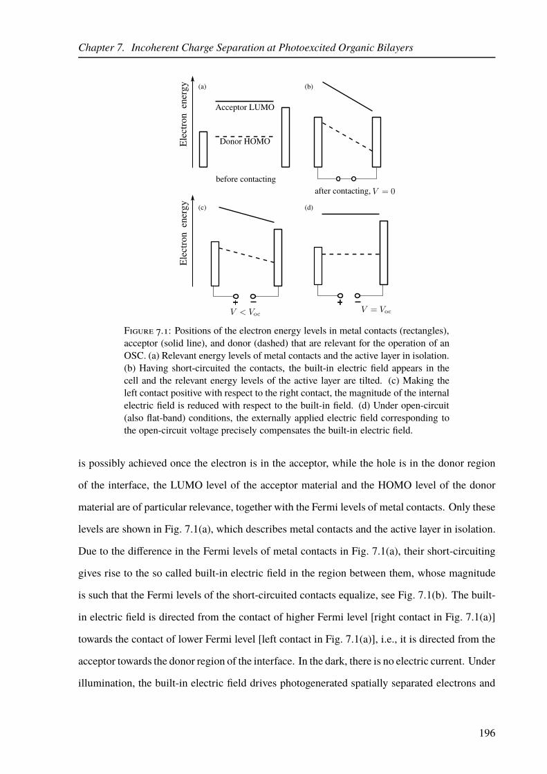
Chapter 7. Incoherent Charge Separation at Photoexcited Organic Bilayers
Acceptor LUMO
Donor HOMO
+ +
before contacting
after contacting,
(a) (b)
(c) (d)
Electron energy
Electron energy
Figure 7.1: Positions of the electron energy levels in metal contacts (rectangles),acceptor (solid line), and donor (dashed) that are relevant for the operation of anOSC. (a) Relevant energy levels of metal contacts and the active layer in isolation.(b) Having short-circuited the contacts, the built-in electric field appears in thecell and the relevant energy levels of the active layer are tilted. (c) Making theleft contact positive with respect to the right contact, the magnitude of the internalelectric field is reduced with respect to the built-in field. (d) Under open-circuit(also flat-band) conditions, the externally applied electric field corresponding tothe open-circuit voltage precisely compensates the built-in electric field.
is possibly achieved once the electron is in the acceptor, while the hole is in the donor region
of the interface, the LUMO level of the acceptor material and the HOMO level of the donor
material are of particular relevance, together with the Fermi levels of metal contacts. Only these
levels are shown in Fig. 7.1(a), which describes metal contacts and the active layer in isolation.
Due to the difference in the Fermi levels of metal contacts in Fig. 7.1(a), their short-circuiting
gives rise to the so called built-in electric field in the region between them, whose magnitude
is such that the Fermi levels of the short-circuited contacts equalize, see Fig. 7.1(b). The built-
in electric field is directed from the contact of higher Fermi level [right contact in Fig. 7.1(a)]
towards the contact of lower Fermi level [left contact in Fig. 7.1(a)], i.e., it is directed from the
acceptor towards the donor region of the interface. In the dark, there is no electric current. Under
illumination, the built-in electric field drives photogenerated spatially separated electrons and
196

Chapter 7. Incoherent Charge Separation at Photoexcited Organic Bilayers
holes in opposite directions, i.e., it promotes the separation of space-separated electron–hole
pairs. In more formal terms, the built-in electric field induces the tilt of the bands, which makes
photogenerated electrons move energetically downwards, towards the contact of higher Fermi
level, while holes move energetically upwards, towards the contact of lower Fermi level, see
Fig. 7.1(b).
The tilt of the bands can be regulated by applying an additional external voltage between the
contacts. The internal electric field in the device is then a superposition of the built-in electric
field and the external electric field. If the left contact is made positive with respect to the right
contact, see Fig. 7.1(c), we say that the so-called forward bias is applied, and the magnitude of
the internal electric field, which determines the slope of the bands, is decreased with respect to
the built-in electric field. At open-circuit conditions, when the potential of the right contact is by
Voc (the so-called open-circuit voltage) higher than the potential of the left contact, the externally
applied electric field exactly compensates the built-in electric field, the bands become flat, while
the current is equal to zero, see Fig. 7.1(d). In this simplistic model, Voc is exactly equal to the
the difference between Fermi levels of the contacts divided by the elementary charge. Further
elevation of the potential difference between the contacts makes us leave the solar-cell operation
regime and enter the operation regime of light-emitting diodes, in which carriers are injected
from the contacts into the active layer. On the other hand, the so-called reverse bias corresponds
to the left contact being negative with respect to the right contact. The reverse bias increases
the internal electric field with respect to the built-in electric field. The carriers generated under
illumination in the reverse-bias regime drift in the strong electric field towards the respective
electrode, and the device works as a photodetector.
The current-voltage characteristic of a solar cell in the dark and under illumination is schemat-
ically presented in Fig. 7.2. In the dark, the current is essentially absent until the contacts start
to inject carriers at voltages that are larger than the open-circuit voltage. Under illumination,
the current flows in the direction opposite to that of the dark current. Maximum photocur-
rent flows under short-circuit conditions (the so-called short-circuit current jsc), the current is
equal to zero at the open circuit, while between these two limits the solar cell generates useful
power. By modulating the voltage between the contacts, the internal electric field in the cell
197

Chapter 7. Incoherent Charge Separation at Photoexcited Organic Bilayers
(b)
(d)
(c)
I
II
Figure 7.2: Current-voltage characteristic (j-current density, V -voltage) of a solarcell in the dark (dashed line) and under illumination (solid line, curve I). The letters(b), (c), and (d) correspond to Figs. 7.1(b), (c), and (d), respectively. The j − Vcharacteristic II is flatter and shows less pronounced electric field-dependence ofthe free-charge generation than the characteristic I.
drops from its maximum value, i.e., the built-in electric field, at short-circuit conditions, to zero
at open-circuit conditions. Typical values of the built-in electric field in OSCs are of the order
of 5×10⁶–107 V/m.
7.2 Experimental and Theoretical Background
7.2.1 Overview of Recent Experimental Results
The standpoint of “hot” charge separation mechanisms, which assume that the conversion of
absorbed photons to free charges is completed within the first ∼ 100 fs after the excitation by
exploiting some form of quantum mechanical coherence, has recently been questioned in a num-
ber of experimental studies. In particular, Vandewal et al. [61] measure the spectral profile of
the IQE, i.e., the IQE as a function of the energy of exciting photons, of a wide range of material
combinations used in OSCs (polymer/fullerene, small-molecule/fullerene, and polymer/polymer
blends). While the IQE spectral profile had been obtained eariler, see, e.g., Ref. [60], Vandewal
et al. succeeded in extending the usually investigated spectral range down to the selective exci-
tation of the lowest-lying “cold” CT state. Measurements in the spectral region that is situated
198

Chapter 7. Incoherent Charge Separation at Photoexcited Organic Bilayers
below the absoprtion regions of individual donor and acceptor materials are extremely challeng-
ing. In simple terms, the oscillator strengths characterizing direct transitions from the ground
state to the low-lying CT states are much smaller than those associated to the direct optical
generation of donor excitons, mainly due to a much smaller overlap between electron and hole
wave functions in CT states. Vandewal et al. overcome the challenge by measuring the inverse
process, i.e., the radiative emission from the CT states to the ground state. Using the emission
spectrum thus obtained, they reconstruct the absorption spectrum of the emissive species by
employing additional theoretical analyses. Here, let us only mention that the theoretical devel-
opments make use of the Boltzmann populations of the ground- and excited-state energy levels
during the emission experiment together with the optical reciprocity theorem. Eventually, the
fraction of photons of energy E that are absorbed is uniquely related to the flux of photons of
energy E that are emitted. The experimental results indicate that, in all the material combina-
tions examined, the efficiency with which the absorbed photons are converted into free charges
does not depend on whether the carriers are generated directly in the “cold” CT state or in some
other higher-energy exciton state. In the most efficient D/A blends, the IQE is around 90% even
when the “cold” CT state is selectively excited.
The experimental findings reported by Vandewal et al. imply that, even though there are ul-
trafast (“hot”, coherent) pathways towards the current-producing pair states, the majority of free
charges that are eventually extracted at the electrodes are obtained on a much longer time scale
in a process that involves the strongly bound and interface-pinned CT state. The relaxation of
the initially generated “hot” CT states is so fast and efficient that the separation predominantly
happens upon reaching the “cold” CT state and is, as such, exclusively determined by the prop-
erties of the “cold” state. This, however, does not necessarily mean that coherent and incoherent
charge separation mechanisms contradict each other. As argued in Ref. [184], both mechanisms
may be at play in most efficient OSCs: free charges are generated on both the ultrashort and
much longer time scales. The study of Vandewal et al. (and to some extent Ref. [184]) simply
suggest that the majority of free carriers are obtained on a long time scale, starting from the
“cold” CT state. However, the driving force that enables the oppositely charged electron and
199

Chapter 7. Incoherent Charge Separation at Photoexcited Organic Bilayers
hole in the “cold” CT state to overcome their mutual Coulomb barrier remains elusive. By mea-
suring the current-voltage (j − V ) characteristics of a number of D/A blends, Vandewal and
coworkers find that, in blends featuring higher IQEs, the j − V characteristics are flatter in the
relevant fourth quadrant (compare curves I and II in Fig. 7.2), while the “cold” states are less
bound and more delocalized compared to blends displaying smaller IQEs [61]. Flat j−V char-
acteristics suggest that the role of the internal electric field in the free-charge generation is only
marginal. Enhancing charge delocalization is proposed to be a promising route towards more
efficient light-to-charge conversion in OSCs.
Further experimental evidence for long-time charge separation out of the “cold” CT state
come from Vithanage et al. [62], who performed measurements on the archetypal P3HT/PCBM
blend by using time-resolved electric field-induced second harmonic method to probe the dy-
namics of the internal electric field with subpicosecond time resolution. The experiment is set
up in the pump–probe configuration, where the pump pulse photogenerates excitons, while the
probe pulse, which acts after a variable time delay, is used to follow the time evolution of the in-
ternal electric field in the blend by measuring the second harmonic generation efficiency. From
the temporal evolution of the experimental signal, the time-dependent electron–hole distance in
the separating charge pair can be extracted. Experimental results demonstrate that the time scale
on which the electron–hole separation exhibits a significant increase in of the order of tens of
picoseconds. On subpicosecond time scales, the electron–hole distance is actually very small
(. 1 nm), which is consistent with the aforementioned ultrafast relaxation of initial “hot” CT ex-
citons towards the bottom of the CT manifold. On a picosecond time scale following photoexcita-
tion, as a results of the quite fast three-dimensional diffusion, the electron–hole pairs evolve into
still bound pairs whose intrapair separations reach several nanometers. On still longer (∼ 100 ps)
time scales, the electrons and holes become free primarily due to the diffusion-controlled sepa-
ration by incoherent hops throughout the respective materials, while the role of the drift in the
internal electric field is only marginal. The authors emphasize the importance of the dimen-
sionality to achieve a fully separated pair state. Namely, in the presence of the disorder, which
induces localization effects, full charge separation is achieved only by circumventing ubiquitous
localized states. This is possible only if one takes into consideration all possible separation paths
200

Chapter 7. Incoherent Charge Separation at Photoexcited Organic Bilayers
an electron and a hole can follow, which can be done correctly only within a three-dimensional
model of a D/A blend. The effect of the dimensionality is also denoted as the entropic effect,
vide infra.
Similar conclusions emerged from the investigation by Devižis et al. [63]. They studied
charge separation at a small-molecule/fullerene bilayer and suggested that, at electric fields typ-
ically encountered within working OSCs, full charge separation is achieved on a ∼ 100 ps time
scale starting from the “cold” CT state. Finally, as has been described in Sec. 6.4, the report by
Grupp et al. [181] also implies that the overwhelming part of separation events takes place out
of the strongly bound and localized CT state.
7.2.2 Overview of Recent Theoretical Results
According to our back-of-the-envelope calculation of the binding energy ǫCTb of the “cold” CT
exciton [see Eq. (1.3)], the depth of the Coulomb barrier that holds together the electron and
hole in this state is of the order of 0.5 eV. Lately, there has appeared a number of theoretical
proposals challenging the common view that the separation from the “cold” CT state requires
surmounting an immense energy barrier [31, 185–187]. All of these studies use thermodynamic
arguments applied to a D/A interface in thermal equilibrium at temperature T and emphasize
the importance of the entropic effect for charge separation. Since the temperature is fixed, the
barrier opposing charge separation is not determined by the difference in (internal) energies E
of the free-charge and “cold” CT state, but rather by the difference in free energies F = E−TS,
where S is the entropy. In this context, the entropy is related to the number of configurations in
which an electron–hole pair, whose electron is in the acceptor, while the hole is in the donor, may
be arranged at a D/A interface. The entropy is, therefore, closely related to the dimensionality;
higher-dimensional interfaces feature more pronounced entropic effects [31, 185]. It is suggested
that the combined effect of entropy and disorder [186] or entropy and carrier delocalization [187]
can substantially reduce (or even eliminate) the Coulomb barrier, so that the electron and hole
in the “cold” CT state are not thermodynamically bound and thus might separate if there are no
kinetic obstacles.
201

Chapter 7. Incoherent Charge Separation at Photoexcited Organic Bilayers
The charge separation from the strongly bound CT state has been extensively studied within
the framework of the Onsager–Braun model [64, 65] and its modifications [188]. Basically, the
separation probability is determined by the competition between the electric field- and temperature-
dependent dissociation of the localized electron–hole pair, which occurs at rate kdiss(F, T ), and
its recombination to the ground state, the lifetime of the pair being τ . The electric field- and
temperature-dependent separation yield ϕ(F, T ) is then equal to
ϕ(F, T ) =1
1 + (kdiss(F, T )τ)−1 , (7.1)
where, within the Onsager–Braun model,
kdiss(F, T ) =3 (µe + µh) e
4πε0εrr3CT
exp
(
− ǫCTb
kBT
)J1(2√−2b
)
√−2b
, (7.2)
b =e3F
8πε0εrkBT. (7.3)
In the last three equations, T is the temperature, while F is the magnitude of the interfacial
electric field. The electron–hole separation in the “cold” CT state is denoted as rCT, µe and
µh are electron and hole mobilities, respectively, while J1 is the Bessel function of order one.
Free parameters in the model are the intrapair separation rCT and the so-called mobility–lifetime
product (µe + µh) τ . The mobility–lifetime product basically describes the competition between
the pair recombination to the ground state and its escape towards free-charge state, which is
assumed to be more probable if the carriers are more mobile. The most important features of the
Onsager–Braun model can be readily appreciated from Eqs. (7.1), (7.2), and (7.3). The model
predicts strong dependence of the separation yield on both the electric field and the temperature.
While the temperature dependence is essentially exponential, see Eq. (7.2), the dependence on
the electric field is more complex.1 The Onsager–Braun model has been revealed successful in
reproducing experimental photodissociation yields in bulk molecular D/A crystals [189], but it
has been recognized as unsuitable for conjugated polymer/fullerene blends [66]. In the following
1At weak fields, it is customary to use the expansionJ1(2√−2b
)
√−2b
= 1 + b+b2
3+
b3
18+ . . .. However, inves-
tigations performed in a broader range of electric field strengths usually prefer to use tabulated values of J1.
202

Chapter 7. Incoherent Charge Separation at Photoexcited Organic Bilayers
paragraphs, we briefly summarize the main reasons for this inadequacy and discuss how the
challenges thus arising have been tackled in the literature.
To start with, the Onsager–Braun model employs the approximation of localized point charge
carriers that does not hold in a conjugated polymer/fullerene blend. In this regard, it has been
proposed that the hole delocalization along conjugated segments of polymer chains can enhance
charge separation [190–192] since the kinetic energy of hole oscillations along chains lowers
the Coulomb barrier between the electron and hole. Another effect that has been recognized as
highly beneficial for charge separation at D/A interfaces is the formation of a dipolar layer at
an interface of two materials with different electron affinities (different LUMO levels). Namely,
experimental studies evidence partial electron transfer from the donor to the acceptor even in the
dark, i.e., in the absence of a photoexcitation [193]. The layers of the partial negative charge in
the acceptor and the partial positive charge in the donor are adjacent to one another, separated by
a distance of the order of a nanometer, and thus form a dipolar layer. Let us assume that polymer
chains are parallel to the D/A interface and that the electron in the “cold” CT state is localized on
an acceptor molecule. The potential energy of the hole residing on the polymer chain adjacent
to the electron localization site is the sum of interaction energies with the electron and with the
partial charges of the dark dipoles. The motion of the hole is then restricted by the presence
of partial positive dipole charges along the chain, which effectively form a potential well. In
the harmonic approximation and on the quantum level, the zero-point energy of the hole in the
potential well can then promote the escape of the hole to the next polymer chain (measured from
the interface) [67, 194]. The combination of the effects due to the hole delocalization and the
presence of dark interfacial dipoles has been demonstrated to reproduce the essential features
of experimental photocurrent data [195]. Furthermore, the combination of the on-chain hole
delocalization and the dimensional (entropic) effects has been suggested as the main reason for
weakly field-dependent and very efficient charge separation at polymer/fullerene bilayers [68].
However, we note that all of the aforementioned studies account for delocalization effects in an
effective way, for example, by introducing the hole effective mass for the on-chain motion [66,
68, 191, 194, 195] or by evenly smearing the charge throughout the delocalization region [190].
203

Chapter 7. Incoherent Charge Separation at Photoexcited Organic Bilayers
Second, in order for the Onsager–Braun model to reproduce experimental data, the mobility–
lifetime product should assume unrealistically high values, meaning that either carrier mobil-
ity or pair lifetime should be unrealistically large. Kinetic Monte Carlo (kMC) studies have
demonstrated that efficient and weakly field- and temperature-dependent charge separation can
be achieved when relevant parameters are carefully chosen on the basis of experimental data [69,
70]. The analysis performed by the authors of Ref. [69] emphasizes that the bulk carrier mobil-
ity and the experimentally measured photoluminescence decay lifetime are not the appropriate
values that should be used in Eq. (7.2). They obtain that the decisive event in the splitting of
the “cold” CT exciton is its escape to the state in which the carriers are not adjacent to the in-
terface, but their separation is somewhat larger, while their recombination becomes improbable.
The escape from the “cold” CT state to this state means that the carriers move on a short length
scale. The mobility value that is appropriate to describe this motion is not the bulk mobility,
which characterizes the motion over long length scales, but rather the terahertz mobility. The
terahertz mobility is typically much larger than the bulk mobility, so that using the bulk mobility
dramatically underestimates the mobility–lifetime product. The correlation between the lifetime
of the photoluminescence signal from the CT state and its lifetime should also be critically as-
sessed. The CT photoluminescence is sensitive to the CT population, which can decrease both
due to the radiative recombination and due to escape of the CT exciton to a free-charge state.
Therefore, in blends in which the CT separation is efficient, the CT photoluminescence decay
lifetime seriously underestimates the actual lifetime of the CT state, because its population is
predominantly depleted by charge separation.
Third, the Onsager–Braun model does not capture the effects of the (energetic and/or spatial)
disorder on charge separation. In Ref. [196], Rubel et al. present an analytical treatment of charge
separation in a one-dimensional disordered chain and conclude that, at least at low interfacial
electric fields, the disorder may enhance the separation of geminate electron–hole pairs. Recent
kMC results also point towards the beneficial role of not too strong energetic disorder on charge
separation [197].
Here, a study on the separation of geminate electron–hole pairs within a one-dimensional
model of a bilayer is presented. Our model takes into account the physical effects that have been
204

Chapter 7. Incoherent Charge Separation at Photoexcited Organic Bilayers
recognized as highly relevant to the process of charge separation, namely the carrier delocaliza-
tion, energetic disorder, electron–hole interaction, carrier recombination, and the interaction of
carriers with the phonon bath and the interfacial electric field. Instead of working in the com-
monly used position space, we transfer the description of charge separation to the space spanned
by the exciton basis states. This transfer permits us to properly account for carrier delocalization
effects. The charge separation is then conceived as a sequence of phonon bath-assisted transi-
tions among different exciton states that starts from a particular state and ends once a free-charge
state is reached.
7.3 Model and Method
7.3.1 Model Hamiltonian
The theoretical model that we employ to describe incoherent charge separation at an organic
bilayer is essentially the same as the model we have used to study ultrafast exciton dynamics in
Ch. 6. A bilayer is modeled by using the one-dimensional multiband semiconductor model that
has been introduced in greater detail in Sec. 6.2. The model Hamiltonian is
H = Hc +Hp +Hc−p +Hc−F, (7.4)
where Hc is the interacting-carrier part of the Hamiltonian that assumes the same form as in
Eq. (6.1), Hp is the free-phonon Hamiltonian given in Eq. (5.2), the carrier–phonon interaction
Hc−p is precisely the same as in Eq. (6.2), whileHc−F describes the interaction of carriers with
the interfacial electric field F that is assumed to be uniform throughout the system
Hc−F =∑
iβi
eF · ri c†iβiciβi
−∑
iαi
eF · ri d†iαidiαi
. (7.5)
In the last equation, ri is the position vector of site i, while vector F is assumed to be perpen-
dicular to the D/A interface and directed opposite the internal electric field of a space-separated
electron–hole pair (in which the electron is in the acceptor, while the hole is in the donor).
205

Chapter 7. Incoherent Charge Separation at Photoexcited Organic Bilayers
There are, however, some important differences between the model used here and the one in
Ch. 6. For example, here, we do take into account the diagonal static disorder, i.e., the on-site
energies of electrons(ǫciβi
)and holes
(ǫviαi
)depend on site index i. The disorder is the essential
element of our model, since disorder-induced localization effects enable us to isolate exciton
states that are similar to states of free charges, as will be detailed in the following.
Similarly to other numerical studies, which obtain charge separation efficiency by tracking
the faith of a single electron–hole pair, we confine ourselves to the single-exciton subspace, see
Sec. 3.5.3. We describe charge separation in the exciton basis, whose basis vectors are stationary
states of an electron–hole pair that are supported by the model interface. Here, the exciton basis
includes the interaction with the internal electric field F, i.e., it is obtained by solving the two-
particle eigenvalue problem (Hc +Hc−F) |x〉 = ~ωx|x〉, which in the basis of single-particle
states localized at lattice sites reads as
∑
i′α′i
j′β′j
(
δii′δαiα′iǫc(jβj)(j′β′
j)− δjj′δβjβ′
jǫv(iαi)(i′α′
i)
− δii′δαiα′iδjj′δβjβ′
j(Vij − qF · (rj − ri))
)
ψx(i′α′
i)(j′β′
j)
= ~ωxψx(iαi)(jβj)
.
(7.6)
Therefore, the exciton basis states contain complete information on the effects of carrier delo-
calization, disorder, and the internal electric field. It is convenient to classify the exciton basis
states in a manner similar to the one we employed in Chapters 5 and 6, where we differenti-
ated between donor exciton states, acceptor exciton states, and space-separated exciton states.
Here, we are interested in full charge separation, which results in almost free carriers capable
of producing electric current. Therefore, we have to individuate exciton states of our model that
resemble these free-carrier states. To this end, we introduce the notion of the contact region of
the bilayer which consists of sites 0, . . . , lc − 1 in the donor part and 2N − lc, . . . , 2N − 1 in
the acceptor part of the bilayer. If both electron and hole are primarily located in the contact
region (the electron in its acceptor part and the hole in its donor part), we consider them as fully
separated carriers. More quantitatively, we say that space-separated exciton state x is a contact
206

Chapter 7. Incoherent Charge Separation at Photoexcited Organic Bilayers
state (state of fully separated carriers) if
lc−1∑
i=0
∑
j
∑
αiβj
|ψx(iαi)(jβj)
|2 ≥ 0.7, (7.7)
and∑
i
2N−1∑
j=2N−lc
∑
αiβj
|ψx(iαi)(jβj)
|2 ≥ 0.7. (7.8)
The space-separated states that are not contact states will be further referred to as CT states.
We point out that the localization induced by disorder is crucial to identify contact states. In
the perfectly ordered system, there are no space-separated states that meet the criteria of spatial
localization given in Eqs. (7.7) and (7.8).
7.3.2 Theoretical Approach to Incoherent Charge Separation
This chapter aims at analyzing the incoherent charge separation, i.e., charge separation that oc-
curs on long time scales so that coherent features are not pronounced and consequently carrier
dynamics can be well described in terms of populations only. Here, we work in the basis of
electron–hole pair states x and study charge separation by finding a stationary solution to an
appropriate equation for populations fx of exciton states. Similarly to Ref. [196], we assume
that contact states act as absorbing states in the course of charge separation, i.e., once an ex-
citon reaches a contact state, it is removed from the system. This removal may be interpreted
as the extraction of the fully separated electron and hole at the electrodes. Instead of studying
charge separation in the commonly used position space, we picture it in the space spanned by
the exciton basis states as a process that starts from an initial state, proceeds through a series
of phonon bath-assisted transitions between exciton states, and finishes once a contact state is
reached. Therefore, we find the stationary solution to equations for populations fx of exciton
states x which do not belong to the group of contact states (further denoted as C). These equa-
tions are Pauli master equations in which the interaction with the phonon bath leads to transitions
between exciton states. The time evolution of the population of exciton state x /∈ C is described
207

Chapter 7. Incoherent Charge Separation at Photoexcited Organic Bilayers
bydfxdt
= gx − τ−1x fx −
∑
x′
wx′xfx +∑
x′ /∈C
wxx′fx′, (7.9)
where gx is the generation rate of state x (the number of excitons generated per unit time in state
x), τx is the lifetime of exciton state x, wx′x is the rate of phonon bath-induced transition from
state x to state x′, while the condition x′ /∈ C on the summation in the fourth term is due to the
assumption of absorbing contact states.
We are searching for the stationary solution f 0x to Eq. (7.9), which satisfies
0 = gx − τ−1x f 0
x −∑
x′
wx′xf0x +
∑
x′ /∈C
wxx′f 0x′ . (7.10)
With the stationary populations of exciton states at hand, we can compute the separation proba-
bility
ϕ =
∑
x′∈C
∑
x/∈C wx′xf0x
∑
x/∈C gx, (7.11)
and the recombination probability
ρ =
∑
x/∈C τ−1x f 0
x∑
x/∈C gx. (7.12)
Using Eq. (7.9), it can be shown that ϕ + ρ = 1. Different choices of gx allow us to investigate
incoherent charge separation starting from different initial states.
The phonon bath-assisted transition rates from exciton state x to exciton state x′, wx′x, can be
obtained using the Fermi golden rule. Let us assume that the sets of oscillators localized on each
lattice site are identical, i.e., in Eqs. (5.2) and (6.2), we assume that index λi, which counts local
oscillators on site i, does not depend on i and can be replaced by λ.2 In the relevant subspace
of single electron–hole excitations, the carrier–phonon interaction can be rewritten as [see also
Eq. (3.85)]
Hc−p =∑
x′xiλ
Γiλx′x |x′〉〈x|
(
b†iλ + biλ
)
, (7.13)
2Actually, our choices of phonon modes and carrier–phonon coupling constants in Chapters 5 and 6 implicitlycontain the same assumption.
208

Chapter 7. Incoherent Charge Separation at Photoexcited Organic Bilayers
where the interaction constants in the exciton basis read as [see also Eq. (6.6)]
Γiλx′x =
∑
βi
∑
jαj
gciβiλψx′∗(jαj)(iβi)
ψx(jαj)(iβi)
−∑
αi
∑
jβj
gviαiλψx′∗(iαi)(jβj)
ψx(iαi)(jβj)
. (7.14)
Therefore, the phonon bath-assisted transition rate from state x to state x′ is
wx′x =2π
~
∑
iλ
|Γiλx′x|2δ(~ωx′ − ~ωx − ~ωλ) n
ph(~ωλ)
+2π
~
∑
iλ
|Γiλx′x|2δ(~ωx′ − ~ωx + ~ωλ)
(1 + nph(~ωλ)
)(7.15)
where nph(E) = (eβE − 1)−1 is the Bose–Einstein occupation number at temperature T =
(kBβ)−1. The right-hand side of Eq. (7.15) can be simplified by further assuming that all the
interaction constants gciβiλand gviαiλ
are independent of site and band indices and are equal to gλ.
Introducing the so-called spectral density J(E) by
J(E) =∑
λ
|gλ|2δ(E − ~ωλ), (7.16)
we obtain
wx′x =2π
~Px′x J(|~ωx′ − ~ωx|)n(~ωx′ − ~ωx), (7.17)
where
Px′x =∑
i
∣∣∣∣∣∣∣∣
∑
jαj
βi
ψx′∗(jαj)(iβi)
ψx(jαj)(iβi)
−∑
jβjαi
ψx′∗(iαi)(jβj)
ψx(iαi)(jβj)
∣∣∣∣∣∣∣∣
2
, (7.18)
whereas
n(E) =
nph(E), E > 0
1 + nph(−E), E < 0
(7.19)
The transition rates wx′x do not depend solely on the energy difference ~ωx′ − ~ωx between ex-
citon states x′ and x, but also on spatial properties (e.g., spatial localization and mutual overlap)
of these states, which is described by quantity Px′x (the so-called spatial proximity factor). The
spatial proximity factor between exciton states of the same character is in general much larger
209

Chapter 7. Incoherent Charge Separation at Photoexcited Organic Bilayers
than the one between states of different characters. In other words, for the same energy difference
~ωx′ − ~ωx, the transition probability wx′x [Eq. (7.17)] is much larger when states x′ and x are
of the same character than when their characters are different. The last point will be repeatedly
used in further discussion.
7.3.3 Parameterization of the Model Hamiltonian
The parameterization of the model Hamiltonian is almost the same as in Ch. 6, where the values
of model parameters are chosen to be appropriate to describe charge separation at the archetypal
regioregular P3HT/PCBM interface in the direction perpendicular to the interface (and polymer
chains). Even though the values of model parameters are selected by using the literature data for
one particular D/A blend, we emphasize that our aim is to unveil fundamental physical effects
responsible for very efficient charge separation at an all-organic bilayer. Therefore, many of
the parameters will be varied (within reasonable limits), and the effects of these variations on
charge separation yield will be rationalized. This is also of practical relevance, since the trends
observed in such variations may suggest which material properties should be tuned in order to
maximize the separation efficiency.
Actual computations are performed on the model system having one single-electron level per
site in the donor and one single-hole level per site in both the donor and acceptor. In order to
mimic the presence of higher-than-LUMO orbitals energetically close to the LUMO level, which
is a situation typical of fullerenes [51, 137], we take two single-electron levels per acceptor site.
While in Ch. 6 we have accounted for the higher-than-LUMO acceptor orbitals that are situated
at ca. 1 eV above the LUMO level, here, motivated by the quite large energy separation between
the lowest-energy PACB state and the lowest-energy donor (or CT) state, we do not consider
these orbitals. The HOMO level of the ordered donor material is taken as the zero of the energy
scale. The model is schematically depicted in Fig. 7.3.
Within each region of the bilayer, the on-site energies of electrons and holes are drawn from
a Gaussian distribution function. For example, the probability density that the energy of the
210

Chapter 7. Incoherent Charge Separation at Photoexcited Organic Bilayers
1.5
2
2.5
Energy
Coordinate
Energ
y (eV
)
DOS (arb. un.)Disorder-averaged
Figure 7.3: Schematic view of the model system indicating different transfer in-tegrals and average on-site energies listed in Table 7.1. The dashed lines representaverage on-site energies, while solid lines represent actual on-site energies, whichvary from site to site due to the diagonal static disorder. The contact region of thebilayer is denoted by rectangles. F is the vector of the interfacial electric field.The plot on the right presents the single-particle DOS for electrons in the isolatedacceptor (full line) and donor (dashed line) regions of the bilayer averaged overdifferent disorder realizations, compare to the similar plot in Fig. 6.1. For eachdisorder realization, the electronic states of the isolated regions are obtained bydiagonalizing the free-electron Hamiltonian [the first term on the right-hand sideof Eq. (6.1)] in which the D/A coupling Jc
DA is set to 0. The DOS for that disorderrealization is computed by broadening each of the single-electron states obtainedby a Gaussian whose standard deviation is equal to 10 meV.
211
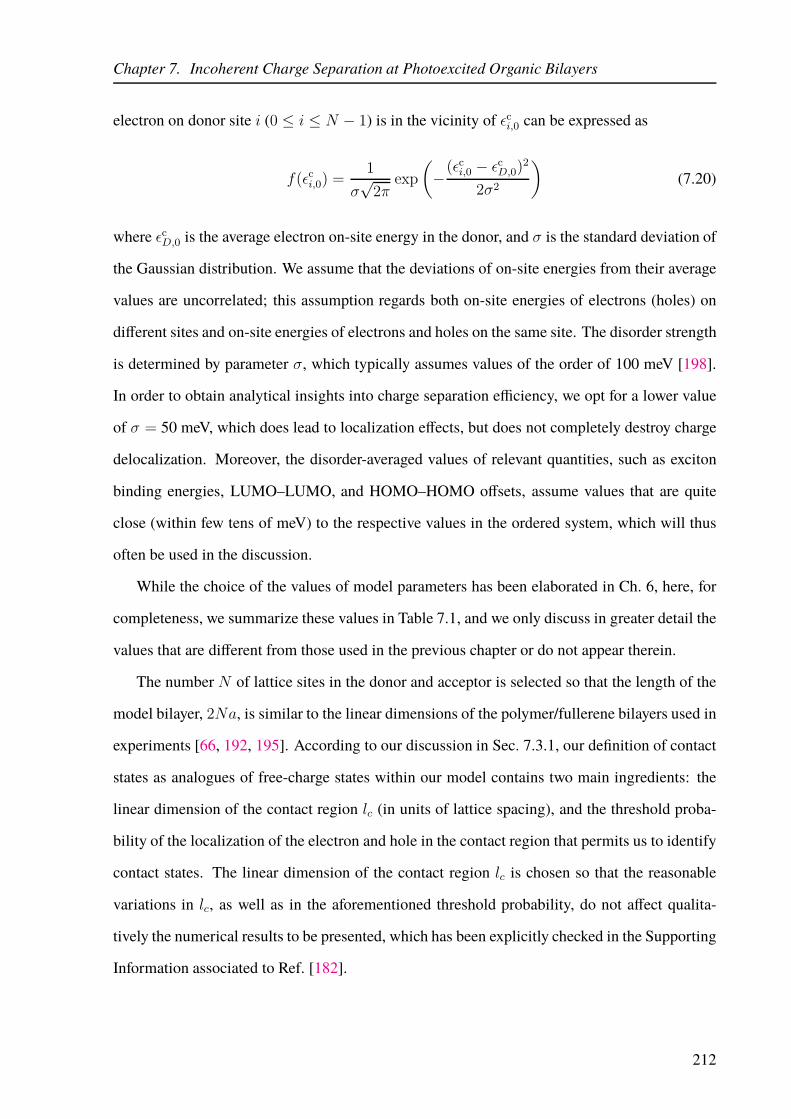
Chapter 7. Incoherent Charge Separation at Photoexcited Organic Bilayers
electron on donor site i (0 ≤ i ≤ N − 1) is in the vicinity of ǫci,0 can be expressed as
f(ǫci,0) =1
σ√2π
exp
(
−(ǫci,0 − ǫcD,0)
2
2σ2
)
(7.20)
where ǫcD,0 is the average electron on-site energy in the donor, and σ is the standard deviation of
the Gaussian distribution. We assume that the deviations of on-site energies from their average
values are uncorrelated; this assumption regards both on-site energies of electrons (holes) on
different sites and on-site energies of electrons and holes on the same site. The disorder strength
is determined by parameter σ, which typically assumes values of the order of 100 meV [198].
In order to obtain analytical insights into charge separation efficiency, we opt for a lower value
of σ = 50 meV, which does lead to localization effects, but does not completely destroy charge
delocalization. Moreover, the disorder-averaged values of relevant quantities, such as exciton
binding energies, LUMO–LUMO, and HOMO–HOMO offsets, assume values that are quite
close (within few tens of meV) to the respective values in the ordered system, which will thus
often be used in the discussion.
While the choice of the values of model parameters has been elaborated in Ch. 6, here, for
completeness, we summarize these values in Table 7.1, and we only discuss in greater detail the
values that are different from those used in the previous chapter or do not appear therein.
The number N of lattice sites in the donor and acceptor is selected so that the length of the
model bilayer, 2Na, is similar to the linear dimensions of the polymer/fullerene bilayers used in
experiments [66, 192, 195]. According to our discussion in Sec. 7.3.1, our definition of contact
states as analogues of free-charge states within our model contains two main ingredients: the
linear dimension of the contact region lc (in units of lattice spacing), and the threshold proba-
bility of the localization of the electron and hole in the contact region that permits us to identify
contact states. The linear dimension of the contact region lc is chosen so that the reasonable
variations in lc, as well as in the aforementioned threshold probability, do not affect qualita-
tively the numerical results to be presented, which has been explicitly checked in the Supporting
Information associated to Ref. [182].
212

Chapter 7. Incoherent Charge Separation at Photoexcited Organic Bilayers
Table 7.1: Values of Model Parameters Used in Computations.
Parameter ValueN 30lc 11
a (nm) 1.0U (eV) 0.65εr 3.0
ǫcD,0 (eV) 2.63Jc,intD,0 (eV) 0.1ǫvD,0 (eV) −0.3Jv,intD,0 (eV) −0.15ǫcA,0 (eV) 1.565ǫcA,1 (eV) 1.865Jc,intA,0 (eV) 0.05Jc,intA,1 (eV) 0.025Jc,extA,01 (eV) 0.02ǫvA,0 (eV) −1.03Jv,intA,0 (eV) −0.15JcDA (eV) 0.1JvDA (eV) −0.1σ (meV) 50
η 1.5Ec (meV) 10τ0 (ps) 250AA/D 0.5T (K) 300
213

Chapter 7. Incoherent Charge Separation at Photoexcited Organic Bilayers
For the spectral density of the phonon bath, we take the Ohmic spectral density [199]
J(E) = ηEe−E/Ec, (7.21)
which is characterized by two parameters: the dimensionless parameter η describes the strength
of the system–bath coupling, while Ec is the energy cutoff determining the energy range of
phonon modes that are strongly coupled to the system. For the Holstein-like system–bath cou-
pling and in the limiting case of a charge carrier localized on a single lattice site, the polaron
binding energy is given by ǫpolb =∑
λ |gλ|2/(~ωλ) [18]. In terms of spectral density J(E), and
specifically for the Ohmic spectral density, the polaron binding energy can be expressed as
ǫpolb =
∫ +∞
0
dEJ(E)
E= ηEc. (7.22)
It is equal to the geometry relaxation energyΛrel upon charging a molecule and to one half of the
reorganization energy Λreorg [18]. In Ref. [51], the relaxation energy of the PC60BM anion was
estimated to be Λrel = 15 meV. The authors of Ref. [200] found that the polaron binding energy
in a long straight polythiophene chain is of the order of 10 meV. We use these estimates and take
the polaron binding energy ǫpolb = 15 meV (the reorganization energy is then Λreorg = 30 meV).
We assume that the system–bath coupling is strongest for the low-frequency phonon modes and
therefore take that Ec = 10 meV and η = 1.5.
There are different kinds of recombination processes that limit the efficiency of OSCs [201].
The recombination of an electron–hole pair that originates from the absorption of a single photon
is geminate recombination. On the other hand, an electron and a hole undergoing a nongeminate
recombination event do not originate from the same photon. Here, we consider only geminate
recombination, which at a D/A interface may occur as (a) the recombination of excitons photo-
generated in a neat donor or acceptor material, or (b) the recombination of excitons in CT states.
The recombination can be further classified as radiative or nonradiative. In neat polymers, re-
combination predominantly occurs via nonradiative processes [127]. In D/A blends, the major
part of charges recombine nonradiatively either at the interface or in the donor material [202].
214

Chapter 7. Incoherent Charge Separation at Photoexcited Organic Bilayers
However, there is no simple model that describes the rate of nonradiative recombination in terms
of microscopic material properties. It is intuitively clear that the smaller is the overlap between
the electron and hole probability densities, the smaller is the rate of their recombination and the
longer is the lifetime of the pair. In previous model studies of charge separation at D/A inter-
faces, the last point has been recognized as the steep dependence of the exciton lifetime on the
electron–hole separation [203], so that the recombination is assumed to occur exclusively from
the strongly bound CT state [195, 196, 203], or a formula describing the aforementioned distance
dependence is proposed [68]. Here, to each exciton state x, be it a state in the neat material or a
CT state, we assign the lifetime τx that is inversely proportional to the weighted overlap of the
electron and hole wave function moduli
τx = τ0
(N−1∑
i=0
|φx,ei |∣∣∣φ
x,hi
∣∣∣ + AA/D
2N−1∑
i=N
|φx,ei |∣∣∣φ
x,hi
∣∣∣
)−1
. (7.23)
In the last expression, the moduli of the wave function of the electron and hole in exciton state
x are defined as
|φx,ei | =
√∑
βi
∑
jαj
∣∣∣ψx
(jαj)(iβi)
∣∣∣
2
, (7.24)
∣∣∣φ
x,hi
∣∣∣ =
√∑
αi
∑
jβj
∣∣∣ψx
(iαi)(jβj)
∣∣∣
2
, (7.25)
while τ0 andAA/D are constants which are determined so that the lifetimes of the lowest CT, XD,
and XA states in the ordered system agree with the values reported in the literature. The expres-
sion for the lifetime given in Eq. (7.23) captures the fact that larger electron–hole overlap favors
faster recombination of the pair. Singlet exciton lifetimes in a variety of conjugated polymers
used in organic solar cells are of the order of hundreds of picoseconds [127]. Time-resolved
photoluminescence measurements yield the singlet exciton lifetime in neat P3HT around 470
ps and in neat PCBM around 740 ps [204]. From the transient absorption measurements per-
formed in blends of P3HT and different fullerenes, the lifetime of the CT state was determined
to be around 3 ns [205]. For the values of model parameters listed in Table 7.1, the lifetime of
the lowest CT state in the ordered system is τ ordCT ∼ 2.5 ns, the lifetime of the lowest XD state
215

Chapter 7. Incoherent Charge Separation at Photoexcited Organic Bilayers
0 0.5 11.2
1.4
1.6
1.8
2
2.2
2.4
0 1 2 0 0.05 0.1 0 1 2 0 1 2
(a) (b) (c) (d) (e)
0CT, CT band 1CT, CT bandcontactXD XA
Energy (eV
)
DOS (arb. un.)
Figure 7.4: Disorder-averaged exciton DOS (in arbitrary units and at F = 0) for(a) donor exciton states, (b) CT states belonging to CT0 band, (c) contact states,(d) CT states belonging to CT1 band, and (e) acceptor exciton states. The hori-zontal arrows in (a) indicate approximate energies of XD states serving as initialstates of charge separation. The vertical double-sided arrow in (b) indicates theenergy range of the CT states acting as initial states of charge separation. TheDOS in a single disorder realization is obtained by broadening each exciton levelby a Gaussian whose standard deviation is equal to 10 meV.
in the ordered system is τ ordXD ∼ 400 ps, and the lifetime of the lowest XA state in the ordered
system is τ ordXA ∼ 800 ps.
7.4 Numerical Results
In this section, we present the results concerning the yield of charge separation starting from
CT and donor states. In all the computations, we average over different disorder realizations
and all the results to be presented are averaged over 256 disorder realizations. In the Supporting
Information associated to Ref. [182], we have checked that averaging over 200–300 disorder
realizations is enough to provide us with convergent results for the separation efficiency. In order
to facilitate the discussion, in Figs. 7.4(a)–(e) we present disorder-averaged DOS for different
groups of exciton states. Similarly as in Ch. 6, we discriminate between CT states belonging to
CT0 and CT1 bands. We say that a CT state belongs to the CT0 (CT1) band if its electron primarily
belongs to the electronic band in the acceptor part of the bilayer arising from the single-electron
level of average energy ǫcA,0 (ǫcA,1), see also the discussion following Eq. (6.9).
216
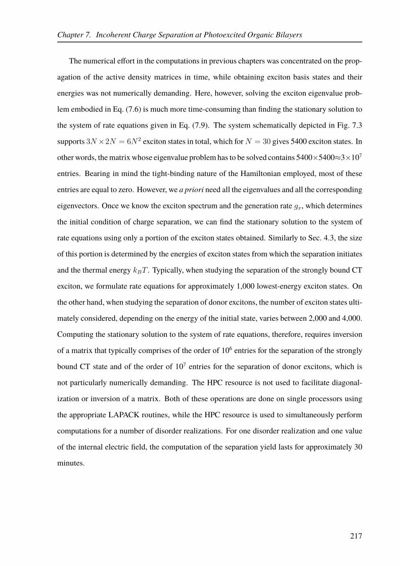
Chapter 7. Incoherent Charge Separation at Photoexcited Organic Bilayers
The numerical effort in the computations in previous chapters was concentrated on the prop-
agation of the active density matrices in time, while obtaining exciton basis states and their
energies was not numerically demanding. Here, however, solving the exciton eigenvalue prob-
lem embodied in Eq. (7.6) is much more time-consuming than finding the stationary solution to
the system of rate equations given in Eq. (7.9). The system schematically depicted in Fig. 7.3
supports 3N×2N = 6N2 exciton states in total, which forN = 30 gives 5400 exciton states. In
other words, the matrix whose eigenvalue problem has to be solved contains 5400×5400≈3×10⁷
entries. Bearing in mind the tight-binding nature of the Hamiltonian employed, most of these
entries are equal to zero. However, we a priori need all the eigenvalues and all the corresponding
eigenvectors. Once we know the exciton spectrum and the generation rate gx, which determines
the initial condition of charge separation, we can find the stationary solution to the system of
rate equations using only a portion of the exciton states obtained. Similarly to Sec. 4.3, the size
of this portion is determined by the energies of exciton states from which the separation initiates
and the thermal energy kBT . Typically, when studying the separation of the strongly bound CT
exciton, we formulate rate equations for approximately 1,000 lowest-energy exciton states. On
the other hand, when studying the separation of donor excitons, the number of exciton states ulti-
mately considered, depending on the energy of the initial state, varies between 2,000 and 4,000.
Computing the stationary solution to the system of rate equations, therefore, requires inversion
of a matrix that typically comprises of the order of 106 entries for the separation of the strongly
bound CT state and of the order of 107 entries for the separation of donor excitons, which is
not particularly numerically demanding. The HPC resource is not used to facilitate diagonal-
ization or inversion of a matrix. Both of these operations are done on single processors using
the appropriate LAPACK routines, while the HPC resource is used to simultaneously perform
computations for a number of disorder realizations. For one disorder realization and one value
of the internal electric field, the computation of the separation yield lasts for approximately 30
minutes.
217

Chapter 7. Incoherent Charge Separation at Photoexcited Organic Bilayers
7.4.1 Charge Separation from the Strongly Bound CT State
As starting states for the charge separation process, here we consider CT states belonging to the
CT0 band. One particular CT state out of all the states in the CT0 band is chosen by requiring
that the mean electron–hole separation defined in Eq. (6.7) be minimal. We will further refer to
such a state as the strongly bound CT state. The strongly bound CT state is located on the lower
edge of the disorder-averaged DOS of CT excitons belonging to the CT0 band, see the vertical
double-sided arrow in Fig. 7.4(b). We set the generation rate gx appearing in Eq. (7.9) to be
different from zero only for the strongly bound CT state.
The field-dependent separation yield from this state is presented by circles in Fig. 7.5(a).
The separation yield is above 0.6 for all the examined values of the electric field down to F = 0.
Figure 7.5(b) presents the low-energy tail of the DOS of contact states [see Fig. 7.4(c)] along
with the distribution of energies of the lowest-energy contact state. Figure 7.5(c) shows the low-
energy tail of the DOS of CT states [see Fig. 7.4(c)] together with the distribution of energies of
the initial strongly bound CT state. The disorder-averaged energy difference between the lowest-
energy contact state and the initial CT state may serve as an estimate of the average energy barrier
that an electron–hole pair in the initial CT state has to surmount in order to reach the nearest
free-charge state. We obtain the average barrier of approximately 0.13 eV (≈ 5 kBT at room
temperature), which is lower (at least by a factor of 2) than usually assumed when considering
separation of the strongly bound CT exciton [34]. Further discussion reveals that the actual
barrier to be overcome is smaller than the energy difference between the lowest-energy contact
state and the initial CT state. Namely, the intermediate CT states, lying between the initial CT
state and the lowest-energy contact state and exhibiting larger electron–hole distances compared
to the initial CT state, are crucial to the successful separation of the initial strongly bound pairs.
Stronger electric field is beneficial to exciton separation which, combined with the fact that the
separation yield is above 0.5 even at F = 0, implies that it exhibits relatively weak dependence
on the magnitude of the electric field.
It is instructive to analyze the results presented in Fig. 7.5(a) from the viewpoint of single
disorder realizations. In Figs. 7.6(a)–(d) we present distributions of the separation yield in single
218

Chapter 7. Incoherent Charge Separation at Photoexcited Organic Bilayers
0 0.05 0.1Relative frequency
0 0.5 1DOS of CT (CT
0) states (arb. un.)
0
0.2
0.4
0.6
0.8
1
105
106
107
Separation yield
Electric field (V/m)
fullsimple
(a)
(b) (c)
00.050.1Relative frequency
1.2
1.4
1.6
Energy (eV
)
00.020.04DOS of contact states (arb. un.)
Figure 7.5: (a) Field-dependent yield of charge separation from the stronglybound CT state. The data labeled by “full” are obtained by numerically solvingEq. (7.9), while the data labeled by “simple” are computed using Eq. (7.32). Thelow-energy edges of the disorder-averaged DOS (full lines) for (b) contact statesand (c) CT states belonging to the CT0 band. The bars depict histograms of thedistribution of the energy of (b) the lowest-energy contact state and (c) the initialstrongly bound CT state. The width of the bins on the energy axis is 10 meV, whileF = 0.
219

Chapter 7. Incoherent Charge Separation at Photoexcited Organic Bilayers
0 0.2 0.4 0.6 0.8 10
0.2
0.4
0.6
0.8
1
Relative frequency
0 0.2 0.4 0.6 0.8 10
0.2
0.4
0.6
0.8
1
0 0.2 0.4 0.6 0.8 1Separation yield
0
0.2
0.4
0.6
0.8
1
Relative frequency
0 0.2 0.4 0.6 0.8 1Separation yield
0
0.2
0.4
0.6
0.8
1
(a) (b)
(c) (d)
Figure 7.6: Histograms showing the distribution of the yield of charge separationfrom the strongly bound CT state for different strengths of the electric field: (a)F = 0, (b) F = 106 V/m, (c) F = 5 × 10⁶ V/m, and (d) F = 107 V/m. The widthof the bins for the separation yield is 0.05.
disorder realizations at different strengths of the electric field. A distinctive feature of all the
histograms is quite small number of disorder realizations for which the separation yield assumes
values in an intermediate range (say between 0.2 and 0.8). Even at zero electric field, the number
of disorder realizations in which the separation yield is high (above 0.8) is greater than the
number of those in which the separation yield is low (below 0.2), which can account for the
mean separation yield above 0.5 even at zero field. As the electric field is increased, the number
of disorder realizations in which the separation yield is low or intermediate decreases, while the
number of disorder realizations in which the separation yield is high increases, see Figs. 7.6(b)–
(d). At F = 107 V/m, the separation yield is between 0.95 and 1 for somewhat less than 90%
of disorder realizations, see Fig. 7.6(d), meaning that the mean yield is close to 1. Relevant to
this discussion are also the relative positions of the lower-energy tails of the DOS of CT states
belonging to the CT0 band and the DOS of contact states, which are presented in the Supporting
Information associated to Ref. [182]. There, we observe that the effect of increasing F on the
DOS tails consists of decreasing the energy difference between the edges of CT and contact
DOS. For sufficiently strong field, the lowest contact state is situated energetically below the
strongly bound CT state.
220
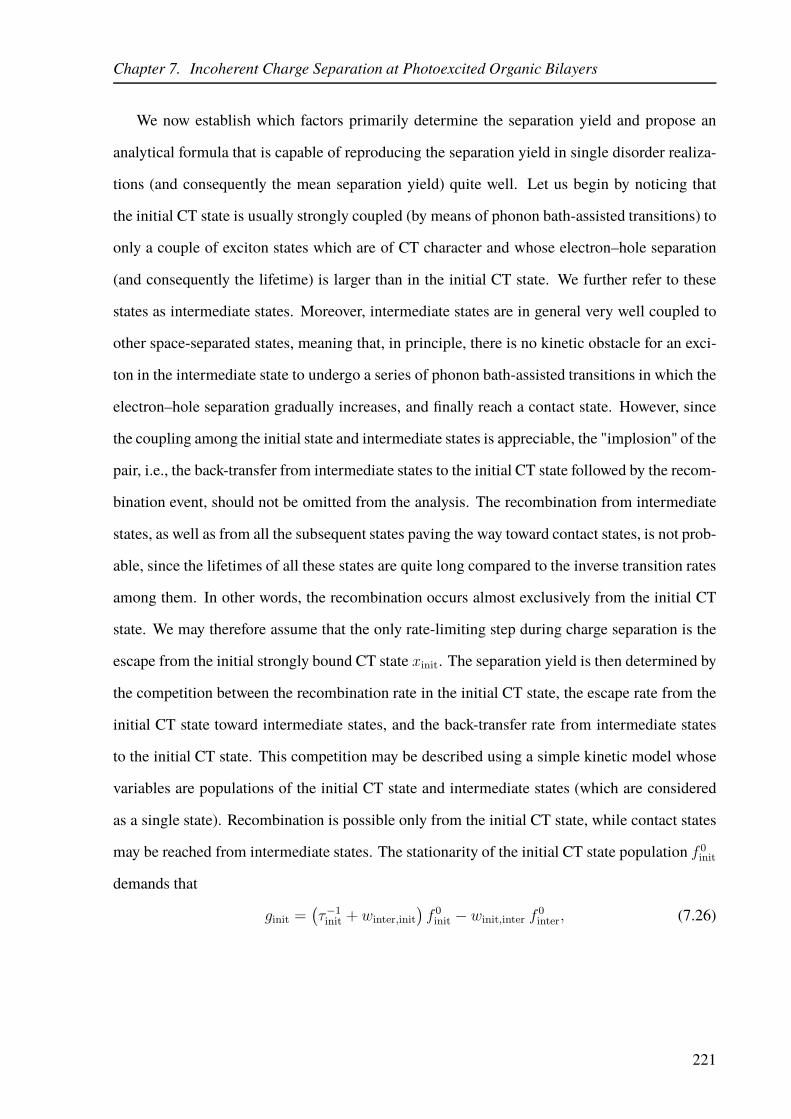
Chapter 7. Incoherent Charge Separation at Photoexcited Organic Bilayers
We now establish which factors primarily determine the separation yield and propose an
analytical formula that is capable of reproducing the separation yield in single disorder realiza-
tions (and consequently the mean separation yield) quite well. Let us begin by noticing that
the initial CT state is usually strongly coupled (by means of phonon bath-assisted transitions) to
only a couple of exciton states which are of CT character and whose electron–hole separation
(and consequently the lifetime) is larger than in the initial CT state. We further refer to these
states as intermediate states. Moreover, intermediate states are in general very well coupled to
other space-separated states, meaning that, in principle, there is no kinetic obstacle for an exci-
ton in the intermediate state to undergo a series of phonon bath-assisted transitions in which the
electron–hole separation gradually increases, and finally reach a contact state. However, since
the coupling among the initial state and intermediate states is appreciable, the "implosion" of the
pair, i.e., the back-transfer from intermediate states to the initial CT state followed by the recom-
bination event, should not be omitted from the analysis. The recombination from intermediate
states, as well as from all the subsequent states paving the way toward contact states, is not prob-
able, since the lifetimes of all these states are quite long compared to the inverse transition rates
among them. In other words, the recombination occurs almost exclusively from the initial CT
state. We may therefore assume that the only rate-limiting step during charge separation is the
escape from the initial strongly bound CT state xinit. The separation yield is then determined by
the competition between the recombination rate in the initial CT state, the escape rate from the
initial CT state toward intermediate states, and the back-transfer rate from intermediate states
to the initial CT state. This competition may be described using a simple kinetic model whose
variables are populations of the initial CT state and intermediate states (which are considered
as a single state). Recombination is possible only from the initial CT state, while contact states
may be reached from intermediate states. The stationarity of the initial CT state population f 0init
demands that
ginit =(τ−1init + winter,init
)f 0init − winit,inter f
0inter, (7.26)
221
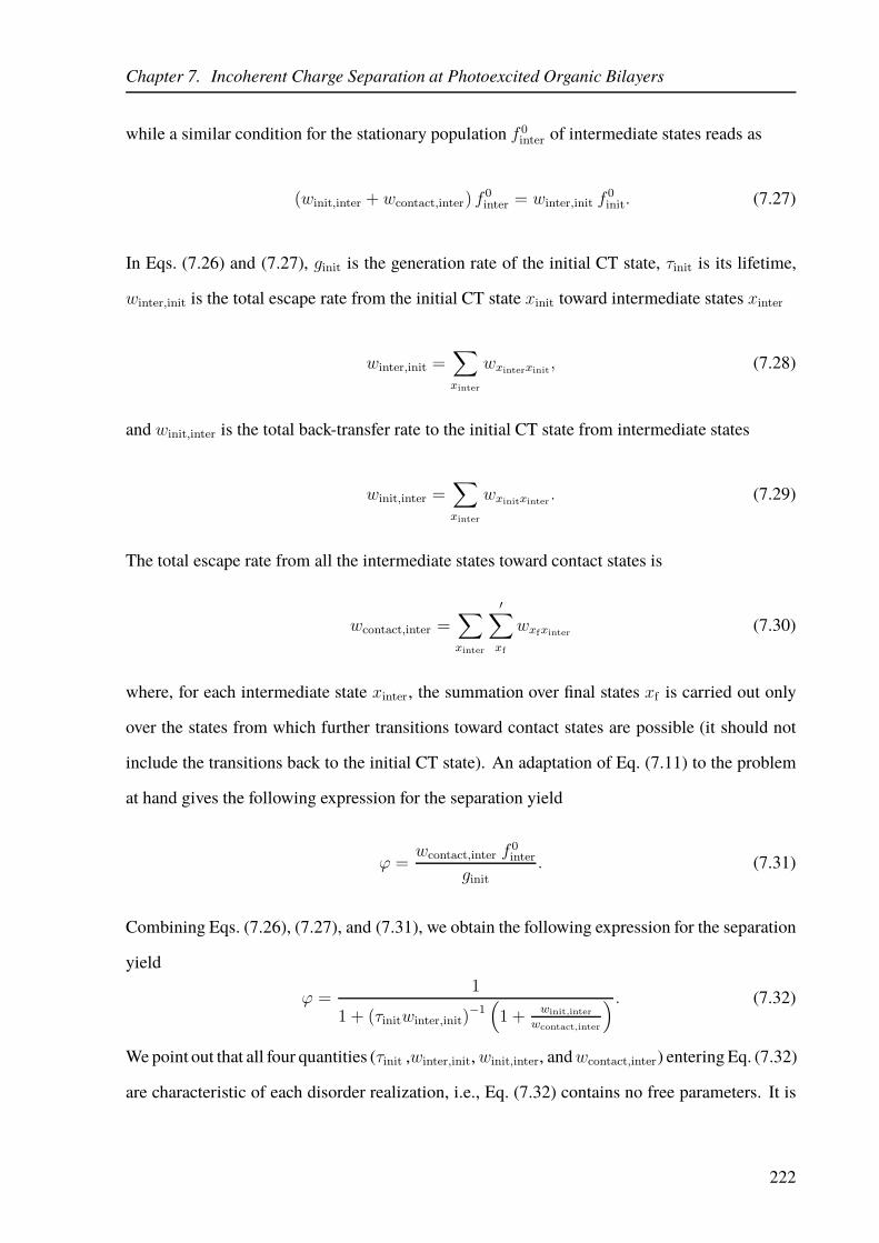
Chapter 7. Incoherent Charge Separation at Photoexcited Organic Bilayers
while a similar condition for the stationary population f 0inter of intermediate states reads as
(winit,inter + wcontact,inter) f0inter = winter,init f
0init. (7.27)
In Eqs. (7.26) and (7.27), ginit is the generation rate of the initial CT state, τinit is its lifetime,
winter,init is the total escape rate from the initial CT state xinit toward intermediate states xinter
winter,init =∑
xinter
wxinterxinit, (7.28)
and winit,inter is the total back-transfer rate to the initial CT state from intermediate states
winit,inter =∑
xinter
wxinitxinter. (7.29)
The total escape rate from all the intermediate states toward contact states is
wcontact,inter =∑
xinter
′∑
xf
wxfxinter(7.30)
where, for each intermediate state xinter, the summation over final states xf is carried out only
over the states from which further transitions toward contact states are possible (it should not
include the transitions back to the initial CT state). An adaptation of Eq. (7.11) to the problem
at hand gives the following expression for the separation yield
ϕ =wcontact,inter f
0inter
ginit. (7.31)
Combining Eqs. (7.26), (7.27), and (7.31), we obtain the following expression for the separation
yield
ϕ =1
1 + (τinitwinter,init)−1(
1 +winit,inter
wcontact,inter
) . (7.32)
We point out that all four quantities (τinit ,winter,init,winit,inter, andwcontact,inter) entering Eq. (7.32)
are characteristic of each disorder realization, i.e., Eq. (7.32) contains no free parameters. It is
222

Chapter 7. Incoherent Charge Separation at Photoexcited Organic Bilayers
0 0.05 0.1Relative frequency
1.15
1.2
1.25
1.3
1.35
1.4
1.45
1.5
00.050.10.15Relative frequency
Ener
gy (eV
)
intermediate CT state initial CT state
(a) (b)
Figure 7.7: Histograms showing distributions of energies of (a) the intermediateCT state (which is most strongly coupled to the initial CT state), and (b) the initialCT state. The histograms are computed for F = 0.
then remarkable that it reproduces quite well the field-dependent separation yield for each disor-
der realization, and consequently the disorder-averaged separation yield, which is presented by
squares in Fig. 7.5(a).
The preceding discussion suggests that the barrier the initial CT exciton has to surmount in
order to reach a contact state is determined by the energy difference ~ωinter−~ωinit between the
initial CT state and the intermediate CT state exhibiting strongest coupling to the initial state. In
Figs. 7.7(a) and (b) we present distributions of energies of the intermediate [Fig. 7.7(a)] and the
initial [Fig. 7.7(b)] CT state at F = 0. We estimate that the average energy difference 〈~ωinter −
~ωinit〉 is around 0.07 eV, which is smaller than the average energy difference between the lowest
contact state and the initial CT state. Therefore, already at F = 0, the average energy barrier
opposing the separation from the initial CT state is ≈ 3 kBT at room temperature. For stronger
F , the height of the barrier decreases, and the barrier is almost eliminated at F & 107 V/m,
when 〈~ωinter − ~ωinit〉 . 10 meV.
Equation (7.32) gives the separation yield which is always an upper bound to the true sep-
aration yield obtained by numerically solving rate equations embodied in Eq. (7.9). Deriving
Eq. (7.32), we assume that there is only one rate-limiting step in the process of charge sepa-
ration from the initial CT state (namely, the escape from the initial CT state to intermediate
states), while further transitions from intermediate states toward contact states occur with cer-
tainty. However, in reality, some of these further transitions may present another obstacle to
223

Chapter 7. Incoherent Charge Separation at Photoexcited Organic Bilayers
full charge separation and, in order to fully reproduce the numerical data, Eq. (7.32) should be
corrected so as to take other rate-limiting steps into account (it turns out that such corrections
are really important only for strong enough disorder, vide infra). We can elaborate more on
the last point by noticing that Eq. (7.32) is actually a version of the Rubel’s formula [196] that
describes the separation of an exciton initially in state 1 through a series of incoherent hops
1 2 · · · n n + 1 among localized states which terminates when free-charge state
n+ 1 is reached
ϕRubel =1
1 + (τ1w21)−1(
1 +∑n
i=2
∏ij=2
wj−1,j
wj+1,j
) . (7.33)
One of the main assumptions behind the Rubel’s formula is that the recombination event is
possible only from the initial CT state 1, its rate being τ−11 . This assumption is satisfied in our
computations, as we obtain that the major part of recombination events occurs from the initial CT
state, so that we may identify τinit in Eq. (7.32) with τ1 in Eq. (7.33). The first rate-limiting step is
the escape from the initial CT state to more separated (and thus longer-lived) intermediate states,
which justifies the identification of winter,init in Eq. (7.32) with w21 in Eq. (7.33). Further rate-
limiting steps are taken into account in Eq. (7.33) by the term∑n
i=2
∏ij=2
wj−1,j
wj+1,jthat takes care of
the fact that, at each step j that has to be completed in order to reach state i, there is a competition
between the escape ratewj+1,j toward the free-charge state n+1 and the back-transfer ratewj−1,j
toward the initial state 1. Rubel et al. have assumed that the pathway from the initial to the final
state is such that hops are possible only between neighboring states in the sequence 1 2
· · · n n + 1, while in our model hops are in principle possible among any two exciton
states. Thus, in our model it is difficult to isolate particular separation paths and ensure that they
do not interfere among themselves. Nevertheless, as evidenced by quite good agreement between
the results presented by circles and squares in Fig. 7.5(a), taking into account only the first
rate-limiting step is a reasonable approximation to the full numerical data. This approximation
is, however, plausible only for not too strong disorder. For stronger disorder, disorder-induced
localization effects become more pronounced and, on its way toward contact states, an exciton
may reach a state exhibiting strong localization. Owing to its strong localization, this state is
poorly coupled to other states, meaning that it may act as another recombination center, or it may
224

Chapter 7. Incoherent Charge Separation at Photoexcited Organic Bilayers
"reflect" excitons toward the initial state, i.e., it acts a trap state for charge separation. Neither
of these two possibilities is captured by Eq. (7.32); therefore, it cannot accurately reproduce the
separation yield for stronger disorder, as we discuss more thoroughly in the next paragraph.
We continue our discussion on the effects of disorder by investigating the separation yield for
different disorder strengths σ at zero electric field. Along with the data emerging from numeri-
cally solving Eq. (7.9), in Fig. 7.8(a) we present the data obtained by means of Eq. (7.32). We
observe that the dependence of ϕ on σ is not monotonic. Namely, for very low values of σ (typ-
ically σ < 20 meV in our one-dimensional model), contact states are generally absent from the
spectrum (the disorder is so weak that disorder-induced localization effects are not pronounced),
and consequently the separation yield within our model is exactly equal to zero in the majority
of disorder realizations. This is different from predictions of other models describing incoher-
ent charge separation [196, 197], according to which the separation yield is different from zero
for all the values of disorder strength down to σ = 0. Therefore, the predictions of our model
are not reliable for too low disorder. Bearing in mind that typical disorder strength in organic
semiconductors is considered to be of the order of 100 meV [198], the aforementioned feature
of our model does not compromise its relevance. For stronger disorder (typically σ > 20 meV),
contact states start to appear in the spectrum and their number grows with increasing σ. At the
same time, the average energy difference 〈~ωinter − ~ωinit〉 between the intermediate state and
the initial CT state decreases, see Fig. 7.8(b), and the escape rate winter,init from the initial CT
state to intermediate states increases [see Eq. (7.17)]. Since the disorder is still not too strong,
further separation from intermediate states is much more probable than the “implosion” of the
pair, meaning that typically winit,inter/wcontact,inter ≪ 1. The last statement, combined with the
fact that τinit essentially does not depend on σ, gives that the separation yield determined by
Eq. (7.32) increases with increasing σ. However, there exists an optimal disorder strength σopt
for which the separation yield attains a maximum value, so that for σ > σopt an increase in
the disorder strength leads to a decreased separation yield. In our numerical computations, σopt
is around 60 meV, in good agreement with results of Ref. [197], which also point towards the
existence of the optimal disorder strength. Although for strong disorder the number of contact
states is large, the pronounced disorder-induced localization starts to impede phonon-assisted
225

Chapter 7. Incoherent Charge Separation at Photoexcited Organic Bilayers
Separation yield
(a)
(b)
simple
40
full
0.2
0.4
0.6
0.8
1
30
40
50
60
70
80
90
0 20 40 60 80 100 120 140 160
Average energy barrier (meV)
Disorder strength (meV)
Disorder strength (meV)0 60 80 100 120 140 16020
0
Figure 7.8: (a) Yield of charge separation from the strongly bound CT state atF = 0 for different strengths σ of the diagonal static disorder. The gray area indi-cates the range of disorder strength in which the predictions of our model are notreliable. The data labeled by ”full“ are obtained by numerically solving rate equa-tions [Eq. (7.9)], while the data labeled by ”simple“ are computed using Eq. (7.32).(b) Average energy barrier 〈~ωinter − ~ωinit〉 between the initial and intermediateCT state as a function of the disorder strength.
226

Chapter 7. Incoherent Charge Separation at Photoexcited Organic Bilayers
transitions among exciton states. The number of trap states for charge separation (cf. previous
paragraph) increases, meaning that there is more than just a single rate-limiting step during the
separation of the initial electron–hole pair. This leads to an increased probability of the “im-
plosion” of the pair into the initial CT state or the pair recombination directly from trap states.
Therefore, the separation yield is decreased. As can be inferred from Fig. 7.8(a), the yield com-
puted using Eq. (7.32) (circles) is again an upper bound to the separation yield obtained by
numerically solving rate equations [Eq. (7.9), squares] and approximates it quite well only for
σ . σopt, while for σ > σopt the two separation yields exhibit opposite trends with increasing
disorder strength. While the true separation yield decreases for σ > σopt, the yield given by
Eq. (7.32) monotonically increases in the entire examined range of disorder strength, consis-
tent with the fact that 〈~ωinter − ~ωinit〉 monotonically decreases with increasing σ. Namely,
Eq. (7.32) does not capture further rate limiting steps in the course of charge separation, and the
highly successful escape from the initial CT state to intermediate states does not guarantee full
charge separation.
The apparent simplicity of our model enables us to systematically study the effects of vari-
ations of different model parameters on the efficiency of charge separation starting from the
strongly bound CT state. Let us first examine how the variations in the electron delocalization
in the acceptor (mimicked by variations in the transfer integral Jc,intA,0 ) and in the hole delocal-
ization in the donor (mimicked by variations in the transfer integral Jv,intD,0 ) affect the separation
yield. We obtain that better delocalization of carriers promotes higher separation yields, see
Figs. 7.9(a) and (b). This can be rationalized using Eq. (7.32), which determines the separation
yield as a function of only a couple of parameters, and following the variation of these param-
eters with varying carrier delocalization. When the separation yield is high [greater than 0.8
already at zero field and for the lowest investigated values of Jc,intA,0 and Jv,int
D,0 , cf. the discussion
of Figs. 7.6(a)–(d)], reasonable variations in Jc,intA,0 and Jv,int
D,0 do not dramatically influence the
separation yield, which remains high. When the separation yield is low or intermediate (less
than 0.8 at zero field and for the lowest investigated values of Jc,intA,0 and Jv,int
D,0 ), it exhibits a
pronounced increase with increasing transfer integrals Jc,initA,0 and Jv,init
D,0 . Namely, better carrier
delocalization leads to an increase in the escape rate winter,init from the initial CT state which,
227

Chapter 7. Incoherent Charge Separation at Photoexcited Organic Bilayers
105
106
107
Separation yield
0
0.2
0.4
0.6
0.8
1
105
106
107
Electric field (V/m)
Separation yield
0
0.2
0.4
0.6
0.8
1
105
106
107
Electric field (V/m)
Separation yield
0
0.2
0.4
0.6
0.8
1
(a)
(b)
(c)
Figure 7.9: Field-dependent separation yield from the strongly bound CT state fordifferent values of (a) the electron transfer integral Jc,int
A,0 in the acceptor, (b) the
hole transfer integral Jv,intD,0 in the donor, and (c) the on-site Coulomb interaction
U .
along with the fact that τinit remains largely unaffected by variations in Jc,initA,0 and Jv,init
D,0 , means
that the separation yield determined by Eq. (7.32) is higher.
Next, we comment on the variations that the separation yield undergoes when the magni-
tude of the on-site Coulomb interaction U is changed. In Fig. 7.9(c) we observe that weaker
electron–hole interaction leads to more efficient charge separation from the strongly bound CT
state. Again, this beneficial effect of weaker Coulomb interaction may be attributed to the
product τinitwinter,init being (on average) larger for weaker Coulomb interaction. On a more
intuitive level, the trends in the separation yield presented in Figs. 7.9(a)–(c) may be rational-
ized by following the changes in the disorder-averaged energy difference 〈~ωinter − ~ωinit〉 with
changing the degree of carrier delocalization and the strength of the electron–hole interaction.
We find that better carrier delocalization and weaker electron–hole interaction favor lower val-
ues of 〈~ωinter − ~ωinit〉, or, in other words, lower the separation barrier from the CT state.
For example, for Jc,intA,0 = 25, 50, and 75 meV, the average energy barrier assumes values of
76, 67, and 55 meV, respectively. Similarly, for U = 0.65, 0.5, and 0.35 eV, 〈~ωinter − ~ωinit〉
is equal to 67, 52, and 33 meV, respectively. Let us also note that each of the effects studied
228

Chapter 7. Incoherent Charge Separation at Photoexcited Organic Bilayers
50 100 150 200 250 3000
0.2
0.4
0.6
0.8
1
0.4 0.6 0.8 10
0.2
0.4
0.6
0.8
1
0.6 0.7 0.8 0.9 11
1.5
2
2.5
3
3.5
4
0.4 0.6 0.8 10
0.2
0.4
0.6
0.8
1
from acceptor states
from donor statesfrom CT states
Temperature (K)
Sep
arat
ion y
ield
Sep
arat
ion y
ield
LUMO-LUMO offset (eV) LUMO-LUMO offset (eV)
Rec
om
bin
atio
npro
bab
ility
(a) (b)
(c) (d)
LUMO-LUMO offset (eV)
Figure 7.10: Yield of charge separation from the strongly bound CT state at zeroelectric field as a function of (a) the temperature, and (b) the LUMO–LUMO offset.(c) The lifetime τinit of the strongly bound CT state as a function of the LUMO–LUMO offset. (d) The probability of recombination from acceptor (circles), donor(squares), and CT (diamonds) states for different values of the LUMO–LUMO off-set. The reported values of the LUMO–LUMO offset refer to the ordered system.Note that the range of LUMO–LUMO offset displayed in panel (c) is narrower thanthat displayed in panels (b) and (d).
can on its own improve the separation from the strongly bound CT state, since its binding en-
ergy strongly depends both on the degree of carrier delocalization and the Coulomb interaction,
compare to the discussion of the results [Figs. 7.13(a)–(c)] concerning charge separation from
the closely separated donor state.
We have also studied the temperature dependence of the process of charge separation from the
strongly bound CT state. We observe an approximately sixfold decrease in the separation yield
when the temperature is decreased from 300 to 100 K, see Fig. 7.10(a). On temperature reduction
from 300 to below 50 K, the separation yield reduces for more than an order of magnitude.
These observations are in agreement with other numerical studies of charge separation from the
strongly bound CT state [70], and with experimentally obtained temperature dependence of the
photocurrent under an excitation at the low-energy edge of the CT manifold [60].
The effect of the variations in the LUMO–LUMO offset on the separation yield is studied
by changing average on-site energies ǫcA,0, ǫcA,1, and ǫvA,0 in the acceptor part of the bilayer by
the same amount, keeping all the other model parameters listed in Table 7.1 unchanged. In first
229

Chapter 7. Incoherent Charge Separation at Photoexcited Organic Bilayers
approximation, these variations manifest themselves in Figs. 7.4(a)–(e) as rigid translations of
the DOS of space-separated exciton states [Figs. 7.4(b)–(d)] with respect to the DOS of donor
and acceptor exciton states [Figs. 7.4(a) and (e)]. Figure 7.10(b) presents the dependence of the
separation yield at zero electric field on the LUMO–LUMO offset. For the LUMO–LUMO offset
greater than approximately 0.5 eV, we observe that the separation yield monotonically decreases
with decreasing the LUMO–LUMO offset, see Fig. 7.10(b). A decrease in the LUMO–LUMO
offset leads to a decreased energy difference between the lowest acceptor (and also donor) state
and the initial CT state, see also Figs. 7.4(a)–(e). We may thus expect that a sufficient decrease
in the LUMO–LUMO offset results in the involvement of acceptor and donor states in the sep-
aration from the strongly bound CT state. The transitions from the space-separated manifold
toward the acceptor (donor) manifold are in general much less probable than the ones inside
the space-separated manifold. However, once an exciton enters the acceptor (donor) manifold,
it can easily recombine, since the typical lifetime of acceptor (donor) states is shorter than the
lifetime of the initial CT state. In other words, the fact that acceptor (donor) states participate
in the separation of the strongly bound CT exciton is seen as a decrease in the separation yield
which is due to the enhanced recombination from acceptor (donor) states. This is clearly seen in
Fig. 7.10(d), which provides data on recombination probability from different groups of exciton
states. While the recombination from acceptor states can partially account for the decrease in
the separation yield observed for LUMO–LUMO offsets below 0.65 eV, see the data represented
by circles in Fig. 7.10(d), the recombination from donor states is reflected in the decrease seen
for LUMO–LUMO offsets below 0.4 eV, see the data represented by squares in Fig. 7.10(d).
Another way to estimate the aforementioned values uses Figs. 7.4(a)–(e) and bears in mind that
the LUMO–LUMO offset for that arrangement of exciton energies is ca. 0.97 eV. Namely, a
rigid translation of Figs. 7.4(b)–(d) by approximately 0.3 eV (upward in energy) makes the ini-
tial CT state energetically close to the acceptor states in the low-energy tail of the acceptor DOS,
meaning that they can participate in the separation of the initial CT state. Similarly, a rigid trans-
lation of Figs. 7.4(b)–(d) by approximately 0.55 eV makes the initial CT state energetically close
to the donor states in the low-energy tail of the donor DOS. However, in order to understand
the behavior of the separation yield in the whole range of LUMO–LUMO offsets displayed in
230

Chapter 7. Incoherent Charge Separation at Photoexcited Organic Bilayers
Fig. 7.10(b), we have to remember that lower LUMO–LUMO offset promotes better coupling
between the two parts of the bilayer, which is mediated by the D/A couplings JcDA and Jv
DA.
As a consequence, when the LUMO–LUMO offset is in the range of 0.6–1 eV, its reduction
enhances the electron–hole overlap in CT states, thus decreasing their lifetime [see Eq. (7.23)
and Fig. 7.10(c)] and increasing the recombination from CT states [see the data represented by
diamonds in Fig. 7.10(d)]. Therefore, enhanced recombination from CT states can explain the
decrease in the separation yield with decreasing LUMO–LUMO offset observed for LUMO–
LUMO offsets above approximately 0.65 eV.
7.4.2 Charge Separation from a Donor Exciton State
Here, we aim at understanding which factors control charge separation starting from a donor
exciton state. In numerical computations, the generation rate gx appearing in Eq. (7.9) is set to
a non-zero value only for donor states. In Chapters 5 and 6, we have noted that the low-energy
(closely separated and strongly bound) donor states are essentially isolated from the manifold
of space-separated states and thus act as trap states for the separation of the initial donor exci-
tons on subpicosecond time scales. On the contrary, higher-energy (more separated and loosely
bound) donor states exhibit appreciable coupling to the space-separated manifold and we may
thus expect that charge separation starting from these states should be more probable than the
one starting from closely separated donor states.
We perform computations of the yield of the separation of donor excitons of different en-
ergies. We focus on the energy windows centered around Einit = 2.0 eV (the optical gap of
the ordered donor material), Einit = 2.1 eV, and Einit = 2.2 eV (significantly above the opti-
cal gap of the ordered donor material), which is indicated by horizontal arrows in Fig. 7.4(a).
Since the precise energies of donor states are determined by the disorder, we choose the initial
donor state among the states that lie in the 50 meV-wide energy windows centered around the
aforementioned energies. One particular donor state out of the chosen states is selected by the
requirement that the squared modulus of the dipole moment for the direct generation of donor
exciton state x, which is proportional to
∣∣∣∣∣
∑
i∈D;αiβi
ψx(iαi)(iβi)
∣∣∣∣∣
2
[see Eq. (6.5)], be maximum. In
231

Chapter 7. Incoherent Charge Separation at Photoexcited Organic Bilayers
0
0.2
0.4
0.6
0.8
1
105
106
107
108
Separa
tion y
ield
Electric field (V/m)
, simple
Figure 7.11: Field-dependent yield of charge separation starting from donor exci-ton states of different energies. The data represented by filled symbols are obtainedby solving the full set of rate equations [Eq. (7.9)]. The data represented by emptycircles are obtained by solving the reduced set of rate equations [Eq. (7.34)] in caseEinit = 2.0 eV.
other words, among donor states in a given energy window, we select the state whose direct
generation from the ground state is most probable. Such a choice of the initial donor state is
motivated by the results presented in Ch. 6, where we have observed that quite high fraction of
photogenerated excitons remain in the initially photoexcited donor state on a picosecond time
scale following the excitation, see, e.g., Figs. 6.11(a)–(l).
In Fig. 7.11, we compare the yields of charge separation starting from donor states of different
energies. As we have expected, charge separation starting from a higher-energy donor state
is more efficient than the one starting from a closely separated donor state. The yield of the
separation from a donor state situated around Einit = 2.2 eV is practically field-independent
and greater than 0.9 for all the examined values of the electric field down to F = 0. The yield
is somewhat higher for Einit = 2.2 eV than for Einit = 2.1 eV. On the other hand, the yield
of the separation from the closely separated donor state (Einit = 2.0 eV) is lower: it is almost
constant for electric fields F . 5 × 10⁷ V/m, its value being around 0.6, after which it rises and
reaches values close to 1 at F ∼ 108 V/m. The value of the electric field at which the separation
from a closely separated donor state occurs with certainty is almost an order of magnitude larger
than in the case of charge separation from the strongly bound CT state, see Fig. 7.5(a), which is
232

Chapter 7. Incoherent Charge Separation at Photoexcited Organic Bilayers
consistent with the fact that the binding energy of the donor exciton is larger than the binding
energy of the CT exciton.
Let us now analyze in more detail the separation of the closely separated donor exciton
(Einit = 2.0 eV). Our data suggest that the major part of recombination events occur from donor
exciton states. This is consistent with the fact that phonon bath-assisted transitions starting from
the closely separated donor exciton state couple it most strongly to other donor states, while cou-
pling to the space-separated manifold is in principle much weaker (we note that its coupling to an
acceptor state is practically negligible). The states of the space-separated manifold to which the
closely separated donor state can couple are typically well spatially separated, long-lived, and
exhibit good coupling to other space-separated states. In other words, despite the weak coupling,
once an exciton in the closely separated donor state performs a transition to the space-separated
manifold, it is highly probable that it will eventually reach a fully separated state. Instead of
finding the stationary solution to the full set of rate equations [Eq. (7.9)] for all exciton states
(excluding contact states), we may compute the separation yield by solving the rate equations in
which we explicitly consider only donor states x ∈ XD and treat exciton states x′ that are not of
donor character as absorbing states
0 = gx − τ−1x f 0
x −∑
x′
wx′xf0x +
∑
x′∈XD
wxx′f 0x′. (7.34)
The separation yield, computed by inserting the solution to Eq. (7.34) into the following expres-
sion for the separation yield [compare to Eq. (7.11)]
ϕ =
∑
x′ /∈XD
∑
x∈XD wx′xf0x
∑
x∈XD gx(7.35)
is presented in case Einit = 2.0 eV by empty circles in Fig. 7.11. We note that the agreement
between the two results (full and empty circles in Fig. 7.11) is quite good, thus validating our
simple picture of charge separation from a low-energy donor state. The same procedure can
be repeated when considering the separation starting from higher-energy donor states, but the
agreement between the results obtained by solving Eq. (7.34) and full system of rate equations
233
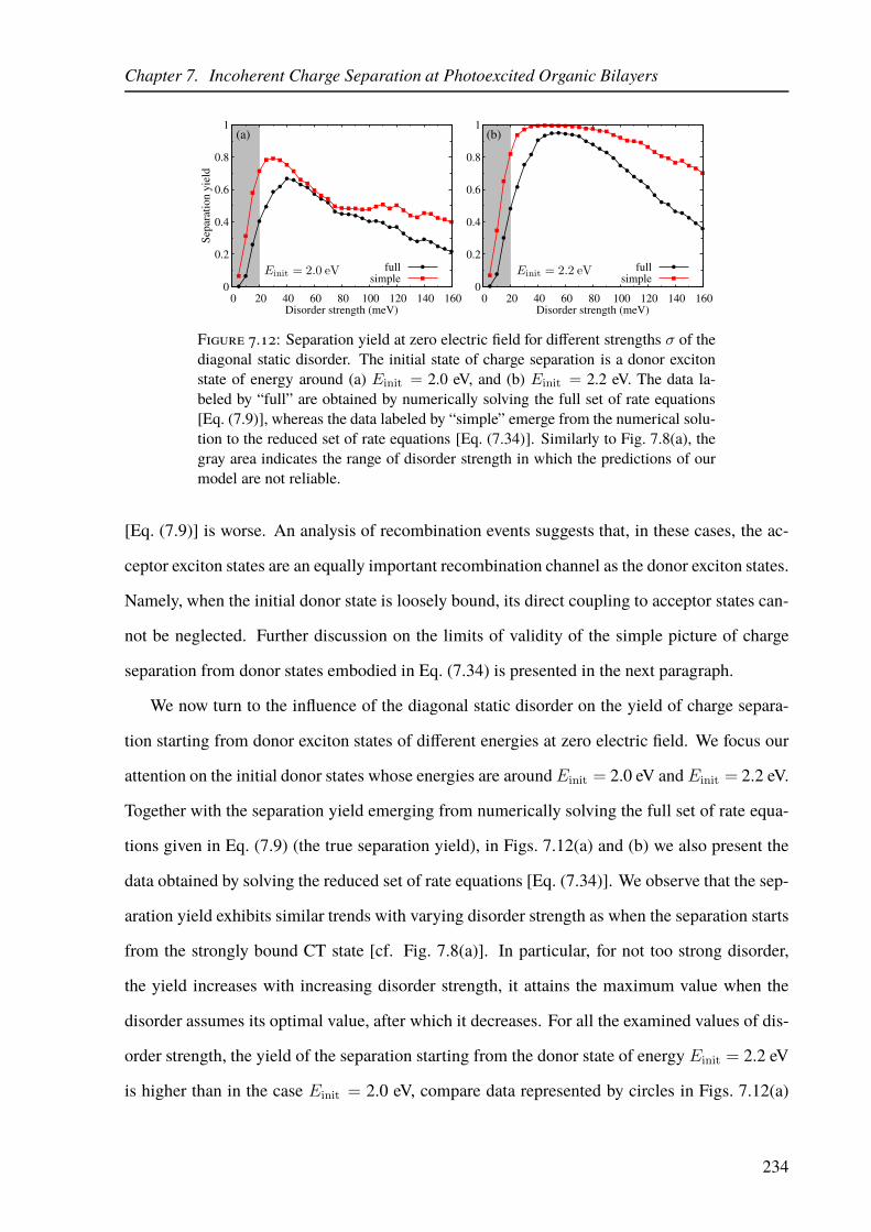
Chapter 7. Incoherent Charge Separation at Photoexcited Organic Bilayers
0
0.2
0.4
0.6
0.8
1
0 20 40 60 80 100 120 140 160
Separation yield
Disorder strength (meV)
fullsimple
0
0.2
0.4
0.6
0.8
1
0 20 40 60 80 100 120 140 160Disorder strength (meV)
fullsimple
(a) (b)
Figure 7.12: Separation yield at zero electric field for different strengths σ of thediagonal static disorder. The initial state of charge separation is a donor excitonstate of energy around (a) Einit = 2.0 eV, and (b) Einit = 2.2 eV. The data la-beled by “full” are obtained by numerically solving the full set of rate equations[Eq. (7.9)], whereas the data labeled by “simple” emerge from the numerical solu-tion to the reduced set of rate equations [Eq. (7.34)]. Similarly to Fig. 7.8(a), thegray area indicates the range of disorder strength in which the predictions of ourmodel are not reliable.
[Eq. (7.9)] is worse. An analysis of recombination events suggests that, in these cases, the ac-
ceptor exciton states are an equally important recombination channel as the donor exciton states.
Namely, when the initial donor state is loosely bound, its direct coupling to acceptor states can-
not be neglected. Further discussion on the limits of validity of the simple picture of charge
separation from donor states embodied in Eq. (7.34) is presented in the next paragraph.
We now turn to the influence of the diagonal static disorder on the yield of charge separa-
tion starting from donor exciton states of different energies at zero electric field. We focus our
attention on the initial donor states whose energies are aroundEinit = 2.0 eV and Einit = 2.2 eV.
Together with the separation yield emerging from numerically solving the full set of rate equa-
tions given in Eq. (7.9) (the true separation yield), in Figs. 7.12(a) and (b) we also present the
data obtained by solving the reduced set of rate equations [Eq. (7.34)]. We observe that the sep-
aration yield exhibits similar trends with varying disorder strength as when the separation starts
from the strongly bound CT state [cf. Fig. 7.8(a)]. In particular, for not too strong disorder,
the yield increases with increasing disorder strength, it attains the maximum value when the
disorder assumes its optimal value, after which it decreases. For all the examined values of dis-
order strength, the yield of the separation starting from the donor state of energy Einit = 2.2 eV
is higher than in the case Einit = 2.0 eV, compare data represented by circles in Figs. 7.12(a)
234

Chapter 7. Incoherent Charge Separation at Photoexcited Organic Bilayers
and (b), which again suggests that excitons initially in higher-energy donor states separate more
efficiently than the ones initially in lower-energy donor states. While the maximum yield of sep-
aration starting from the donor state of energy Einit = 2.0 eV is around 0.7, the maximum yield
in the case Einit = 2.2 eV is above 0.9. For both initial states of charge separation, the yield
computed by numerically solving the reduced set of rate equations [squares in Figs. 7.12(a) and
(b)] is an upper bound to the true separation yield [circles in Figs. 7.12(a) and (b)] for all the
examined values of σ. For Einit = 2.0 eV, the separation yield computed by solving the re-
duced set of rate equations reproduces the true separation yield very well when the disorder
strength is from around 40 meV to around 90 meV, while for stronger disorder the agreement
between the yields computed in two manners deteriorates. This suggests that, for moderate dis-
order strength, our simple picture of charge separation from the closely separated donor state,
embodied in Eq. (7.34), is plausible. At stronger disorder, the localization effects become more
important and recombination may occur from states that do not belong to the donor manifold as
well. On the other hand, the agreement between the two separation yields in case Einit = 2.2 eV
is less satisfactory than in case Einit = 2.0 eV, see Fig. 7.12(b).
We also examine the dependence of the separation yield starting from the closely separated
donor state on the magnitude of electron (Jc,intD,0 ) and hole (Jv,int
D,0 ) transfer integrals in the donor
part of the bilayer. We find that reasonable variations in these quantities do not induce major
changes in the separation yield, see Figs. 7.13(a) and (b), which stands in contrast to the beneficial
effect that better charge delocalization has on the separation of the strongly bound CT exciton,
see Figs. 7.9)(a) and (b). The reason for this behavior is the fact that the donor exciton binding
energy, which is a rough measure of the energy barrier which has to be overcome in order for
free charges to form, is not strongly dependent on the carrier delocalization in the donor. The
factor that primarily determines the binding energy of the donor exciton is the strength of the
Coulomb interaction. Figure 7.13(c) presents the field-dependent separation yield for different
values of the on-site Coulomb interaction U . As anticipated, we find that lowering U leads to a
higher separation yield.
The temperature-dependent separation yield at zero electric field is shown in Fig. 7.14(a).
We see that lower temperature leads to lower separation yield since the phonon bath-assisted pro-
235

Chapter 7. Incoherent Charge Separation at Photoexcited Organic Bilayers
105
106
107
108
0
0.2
0.4
0.6
0.8
1
Separation yield
105
106
107
108
Electric field (V/m)
0
0.2
0.4
0.6
0.8
1
Separation yield
105
106
107
108
Electric field (V/m)
0
0.2
0.4
0.6
0.8
1
Separation yield
(a)
(b)
(c)
Figure 7.13: Field-dependent yield of charge separation starting from the closelyseparated donor exciton state (Einit = 2.0 eV) for different values of (a) the electrontransfer integral Jc,int
D,0 in the donor, (b) the hole transfer integral Jv,intD,0 in the donor,
and (c) the on-site Coulomb interaction U .
50 100 150 200 250 3000
0.2
0.4
0.6
0.8
1
0.4 0.6 0.8 10
0.2
0.4
0.6
0.8
1
0.4 0.6 0.8 10
0.2
0.4
0.6
0.8
1
from donor statesfrom acceptor states
from CT states
(a)
(b)
(c)
Temperature (K)
Separation yield Separation yield
LUMO-LUMO offset (eV)
LUMO-LUMO offset (eV)
Recombination
probability
Figure 7.14: Yield of charge separation starting from the closely separated donorstate (Einit = 2.0 eV) at zero electric field as a function of (a) the temperature, and(b) the LUMO–LUMO offset. (c) The recombination probability from donor (cir-cles), acceptor (squares), and CT (diamonds) states as a function of the LUMO–LUMO offset. The reported values of the LUMO–LUMO offset refer to the or-dered system. In panel (b), we present results in which acceptor states are included(Jv
DA 6= 0) and excluded (JvDA = 0) from the computation.
236

Chapter 7. Incoherent Charge Separation at Photoexcited Organic Bilayers
cesses transferring an exciton in a donor state to the space-separated manifold (and, eventually,
to a state of fully separated charges) are weaker. The separation yield exhibits a sixfold decrease
when the temperature is lowered from the room temperature to around 50 K. The intensity of the
temperature variation-induced effect on the separation yield is somewhat smaller than in case of
the separation starting from the strongly bound CT state, compare to Fig. 7.10(a).
In the end, we examine how the value of the LUMO–LUMO offset affects charge separation
from the closely separated donor state. Figure 7.14(b) presents the separation yield as a function
of the LUMO–LUMO offset for the values of model parameters listed in Table 7.1 (JvDA 6= 0,
circles), as well as for JvDA = 0 (squares), i.e., when states of acceptor excitons are excluded
from the computation. For the LUMO–LUMO offset above approximately 0.6 eV, we observe
that the separation yield in both cases is essentially the same and weakly dependent on the par-
ticular value of the LUMO–LUMO offset. This indicates that, in this range of LUMO–LUMO
offsets, charge separation starting from the closely separated donor state does not involve accep-
tor exciton states, which once again validates our simple picture of charge separation from that
state [formally embodied in Eq. (7.34)]. However, when the LUMO–LUMO offset is below 0.6
eV, the separation yield in case JvDA 6= 0 starts to decrease with decreasing the LUMO–LUMO
offset. On the other hand, in case JvDA = 0, similar decrease in the separation yield is observed
only when the LUMO–LUMO offset is lower than approximately 0.4 eV. The different behavior
of the separation yield in the two cases signalizes that, when the LUMO–LUMO offset assumes
values lower than ca. 0.6 eV, states of acceptor excitons are involved in charge separation and
the observed decrease is due to the recombination from acceptor states. As we have already
noted in the analysis of Fig. 7.10(b), when the LUMO–LUMO offset is around 0.6 eV, the low-
energy tails of the CT and acceptor exciton DOS become energetically close. Further analysis
of recombination events from different groups of exciton states, whose results are reported in
Fig. 7.14(c), shows that the contribution of the recombination from acceptor states to the total
recombination probability becomes appreciable when the LUMO–LUMO offset is around 0.6
eV. When acceptor states are excluded from the computation, the independence of the separa-
tion yield on the LUMO–LUMO offset can be inferred from the flat recombination probability
from the donor states [circles in Fig. 7.14(c)], which is disturbed when the energy of the strongly
237

Chapter 7. Incoherent Charge Separation at Photoexcited Organic Bilayers
bound CT state is approximately equal to the energy of the initial donor state, which occurs for
the LUMO–LUMO offset below around 0.4 eV. For even smaller values of the LUMO–LUMO
offset, all the space-separated states are energetically above the initial donor state, meaning that
full charge separation can be achieved only by means of energetically-upward processes. The de-
crease in the separation yield with decreasing the LUMO–LUMO offset can then be attributed to
an increased probability of recombination from donor states, which is clearly seen in Fig. 7.14(c).
7.5 Discussion and Significance of Our Results
Using a one-dimensional model of an all-organic bilayer, we have modeled and investigated the
process of incoherent charge separation out of CT and donor exciton states. The main advantage
of our model over existing approaches is that it properly takes into account carrier delocaliza-
tion, whose importance for efficient charge separation in OPV systems has been repeatedly rec-
ognized [66, 68, 190, 191, 194, 195]. The carrier delocalization is fully and naturally taken into
account by working in the exciton basis, rather than in the commonly used position basis. The
charge separation is then conceived as a sequence of environment-assisted transitions among
exciton basis states that terminates once a free-charge state is reached. Another important ingre-
dient of our model is the diagonal static disorder, which is crucial to identify the counterparts of
free-charge states within our description.
Many of the studies mentioned in Sec. 7.2 underline the beneficial role played by the system’s
dimensionality in the conversion of strongly bound excitons to free charges. Therefore, com-
ments on our results in view of the reduced dimensionality of our model are in order. Although
formally one-dimensional, the proposed model of a bilayer can be regarded as a two- (or three-)
dimensional model consisting of periodically repeated linear systems identical to the one shown
in Fig. 7.3 that are isolated from each other, i.e., the transfer integrals between (neighboring)
linear systems are equal to zero. We have established that, within our one-dimensional model,
the degree of charge delocalization, quantified by the values of the electron and hole transfer
integrals, is one of the factors influencing the (CT exciton) separation efficiency, see Figs. 7.9(a)
and (b). On simple grounds, better delocalization is beneficial to charge separation because it
238

Chapter 7. Incoherent Charge Separation at Photoexcited Organic Bilayers
increases the mean distance (in the direction of a single linear system, which is perpendicular to
the D/A interface) between the electron and hole located in the acceptor and donor, respectively.
If we assigned nonzero values to transfer integrals coupling different linear systems, the charges
could also delocalize along the direction perpendicular to the linear systems (parallel to the D/A
interface) and further increase their separation. Therefore, it may be expected that the separa-
tion yield would be enhanced in such genuinely two- (or three-) dimensional model. This line
of reasoning is supported by studies highlighting the beneficial role of hole delocalization along
polymer chains in charge separation [68, 191], particularly if we keep in mind that the values
of the intrachain transfer integrals are typically larger than the ones employed in this study. We
may also say that the separation yields we obtain using an effectively one-dimensional model
are the lower limit to the ones that would be obtained in a higher-dimensional system. Another
possible interpretation of our results is that they suggest that, in order to describe fundamental
reasons for efficient charge separation at all-organic bilayers, it is more important to properly
account for charge delocalization than for dimensionality effects.
Next, we discuss our assumptions concerning the strength of the carrier–bath interaction.
We take that the polaron binding energy is ǫpolb = 15 meV, which is significantly lower than
values commonly reported in electronic-structure studies of single PCBM molecules [20, 168].
The selection of the values of model parameters implicitly suggests that each lattice site may be
imagined to substitute a polymer chain or a group of fullerene molecules. In this regard, carrier
transfer from one site to another should not be interpreted as transfer between single molecules
supporting localized carrier states, but rather as transfer between two aggregates of molecules
supporting delocalized carrier states. It has been demonstrated recently that, in such a case, the
definition of ǫpolb [given in the text between Eqs. (7.21) and (7.22)] should be corrected so as to
take into account delocalization effects, which can substantially reduce ǫpolb [206]. Having all
these things considered, we believe that our choice of the magnitude of ǫpolb is reasonable. Larger
ǫpolb (while keeping all other model parameters fixed) would result in a higher separation yield,
because the phonon bath-induced transition rates [Eq. (7.17)] would be larger. In this sense, our
results may also be regarded as the lower limit to the separation yield computed for larger ǫpolb .
Another common choice for the spectral density J(E) [Eq. (7.16)] when studying charge
239

Chapter 7. Incoherent Charge Separation at Photoexcited Organic Bilayers
separation in photosynthetic [199] and OPV systems [58, 207] is the so-called Drude–Lorentz
spectral density
JDL(E) =2
π∆
E · ~γE2 + (~γ)2
, (7.36)
which is characterized by two parameters, ∆ and ~γ. According to the relation between the
spectral density and the polaron binding energy embodied in Eq. (7.22), parameter ∆ represents
the polaron binding energy, whereas ~γ determines the energy range of bath modes whose cou-
pling to the system is appreciable. While the behavior of the Ohmic spectral density [Eq. (7.21)]
at large energies (E ≫ Ec) is essentially exponential, the Drude–Lorentz spectral density de-
creases only algebraically forE ≫ ~γ. Therefore, the Drude–Lorentz spectral density generally
favors coupling to a wider range of phonon modes than does the Ohmic spectral density em-
ployed in our numerical computations. It is then not surprising that the Drude–Lorentz spectral
density promotes even higher separation yields than the Ohmic spectral density, which has been
demonstrated in the Supporting Information associated to Ref. [182].
Our principal conclusion is that the synergy between moderate energetic disorder and carrier
delocalization can explain quite high and relatively weakly field-dependent separation efficien-
cies observed in solar cells photoexcited at the low-energy edge of the CT manifold [61], see
Fig. 7.5(a). At electric fields typically encountered in a working organic solar cell (F ∼ 5–
10 V/µm), the efficiency of the separation of the strongly bound CT exciton is above 0.8. Our
analytical treatment, which is sensible for not too strong disorder, reveals that the separation of
the strongly bound CT exciton is actually governed by the competition between the recombina-
tion from the initial CT state and the escape towards more separated and long-lived intermedi-
ate CT states, from which further separation proceeds without kinetic obstacles, see Eq. 7.32.
Strong disorder destroys this simple picture, and the appearance of well-separated and strongly
localized states following the intermediate states prevents electron–hole pairs from eventually
reaching contact states. Our finding that better charge delocalization promotes more efficient
separation of the strongly bound CT exciton further corroborates the conclusions of Ref. [61],
which emphasize that, in the most efficient OSCs, the strongly bound CT state is only weakly
bound and quite delocalized. Moreover, we observe a much milder temperature dependence of
240

Chapter 7. Incoherent Charge Separation at Photoexcited Organic Bilayers
the separation yield [see Fig. 7.10(a)] than the (predominantly) exponential one predicted by
the Onsager–Braun model, see Eqs. (7.1), (7.2), and (7.3), in agreement with experimental [60]
and theoretical studies [70]. The fact that larger LUMO–LUMO offsets favor more efficient
free-charge generation out of the strongly bound CT state is attributed to an increased recombi-
nation probability from acceptor and donor states observed for smaller LUMO–LUMO offsets,
see Figs. 7.10(b) and (d).
The separation of donor excitons is also quite efficient, and its yield depends on the exciton
energy, see Fig. 7.11. The electric field required to separate the closely separated donor exciton
with certainty is almost an order of magnitude higher than the one needed to separate the strongly
bound CT exciton. Our results suggest that the separation of the closely separated donor exciton
exhibits only one rate-limiting step, i.e., the escape to the space-separated manifold. Carrier
delocalization does not strongly influence this escape, see Figs. 7.13(a) and (b). The donor
exciton separation shows weak temperature dependence, see Fig. 7.14(a), while its decrease with
decreasing the LUMO–LUMO offset is attributed to the recombination from acceptor states, see
Figs. 7.14(b) and (c). Relatively weak disorder is beneficial to donor exciton separation, while
strong disorder suppresses it, see Figs. 7.12(a) and (b).
In summary, our results provide unambiguous evidence that efficient charge separation can
be achieved even out of strongly bound pair states and are supported by experiments [61, 181]
suggesting that free-charge generation predominantly occurs on long time scales, from localized
initial conditions.
241

Chapter 8
Conclusion
This thesis presents a detailed account of the fundamental physical mechanisms that govern the
dynamics of photoinduced electronic excitations in D/A OSCs. Even though an ever-growing
power of computational facilities has enabled us to depict microscopic processes occurring in
a variety of materials with an unprecedented temporal and spatial resolution, their fundamental
physical understanding still lacks. Therefore, in this thesis, we concentrate on apparently sim-
ple, but physically grounded, model Hamiltonians, while comprehensive investigations of their
dynamics provide us with important insights that will be once again briefly summarized in the
following text.
Organic semiconductors are physical systems whose theoretical description is quite challeng-
ing because their basic properties are very different from those of inorganic semiconductors, the
theoretical study of which was one of the milestones of the 20th-century physics. The electronic
energy bands in typical organic semiconductors are narrow, the dielectric screening is weak, the
coupling of carriers to lattice vibrations in strong, while the disorder is omnipresent. Instead
of creating free carriers, an optical excitation of an organic semiconductors creates Coulomb-
correlated strongly bound electron–hole pairs, i.e., excitons. A sensible description of the light-
to-charge conversion by means of organic semiconductors requires that a number of physical
effects be treated simultaneously and on equal footing. Moreover, experimental findings indi-
cating an ever-faster time scale of the light-to-charge conversion in the most efficient OSCs [36–
38] demand that the theoretical treatment be fully quantum.
The starting point for our study is the rather general standard semiconductor Hamiltonian that
242
Chapter 8. Conclusion
explicitly takes into account carrier delocalization, electron–hole interaction, carrier–phonon in-
teraction, and the interaction with an external optical field, see Ch. 2. The model Hamiltonian
can, under certain approximations, be reduced to the well-known Wannier and Frenkel exciton
models, but is actually more general than them. The fully quantum and statistical treatment of
the dynamics triggered by a pulsed optical excitation of the model system relies upon the density
matrix formalism, see Ch. 3. The carrier branch of the infinite hierarchy of mutually coupled
equations describing the temporal evolution of density matrices is truncated by employing the
DCT scheme up to the second order in the exciting field. The second order is the lowest order
in the exciting field in which excitonic effects can be conclusively studied, and, as we have de-
scribed, the respective truncation is intimately related to the low-density limit, i.e., to confining
the dynamics to the single-exciton subspace. From the methodological point of view, our main
contribution regards the truncation of the phonon branch of the hierarchy. Guided by the energy
and particle-number conservation laws, which have to be met once the pulsed excitation has
vanished, we perform a specific truncation of the phonon branch on the level of single-phonon-
assisted density matrices. Although such a treatment of the carrier–phonon coupling precludes
us from treating polaronic effects, which are sometimes considered as highly important in or-
ganic semiconductors, recent theoretical results suggesting that charge carriers in these systems
are of nonpolaronic nature make our approach sensible.
Theoretical investigations of the exciton formation and initial stages of exciton relaxation in
the model of a neat organic semiconductor reveal that these processes happen on a multitude
of time scales, see Ch. 4, which has also been observed experimentally [46, 47]. In greater de-
tail, our numerical computations, which capture processes occurring on picosecond or shorter
time scales, suggest that the initially generated coherent exciton populations are transformed
into incoherent ones on a ∼ 50-fs time scale, which is followed by the build-up of the Coulomb
correlation and the formation of bound electron–hole pairs on a ∼ 500-fs time scale. The ul-
trafast stages of exciton relaxation dynamics are observed on a picosecond time scale. Despite
the fact that our model contains some oversimplifications, the time scales emerging from our
computations are consistent with the experimental ones.
243
Chapter 8. Conclusion
Our study of ultrafast exciton dynamics in photoexcited D/A interfaces has provided rele-
vant insights into the origin of spatially separated charge carriers that have been experimentally
observed on such short time scales, see Ch. 5. Our approach to the problem considers exciton
generation by means of an optical excitation, exciton dissociation, and further charge separa-
tion on equal footing and on a fully quantum level. The common interpretation of the results of
ultrafast time-resolved spectroscopic studies indicates that states of spatially separated charges
become populated on a ∼ 100-fs time scale by means of the ultrafast population transfer from
the initially excited donor exciton states [36–38]. Our results, however, demonstrate that the
main source of space-separated charges on ∼ 100-fs time scales is their direct optical generation
from the ground state. Such a route towards space-separated charges is possible due to the redis-
tribution of oscillator strengths among donor and space-separated states, which is mediated by
their resonant “hybridization”. Previous proposals that the long-range charge separation in D/A
OSCs may be achieved through the direct optical generation of space-separated pairs [143, 144]
were motivated by the studies of the absorption spectrum of D/A interfaces, which identified the
aforementioned absorption intensity redistribution, but were unable to fully appreciate its actual
relevance. Our work, therefore, complements these studies by examining the ultrafast exciton
dynamics triggered by the excitation of a D/A interface and is capable of demonstrating that the
direct optical generation of space-separated charges is their main source on ultrafast time scales.
We also embark on the theoretical treatment of ultrafast time-resolved transient absorption
spectroscopy. By combining our approach to the ultrafast exciton dynamics with recent theo-
retical developments concerning the computation of the differential transmission signal [157],
we derive an analytical expression for the signal that explicitly demonstrates that both popula-
tions and coherences, rather than only populations, are expected to govern experimental signals
on subpicosecond time scales. Our numerical computations of differential transmission signals
reveal that, in some cases, the signal is expected to predominantly originate from coherences
between exciton states and the ground state, which seriously challenges its usual interpretations
in terms of population transfer.
The conclusions underlined in the last two paragraphs do not necessarily imply that there
is no population transfer from initially generated donor towards space-separated states. Indeed,
244

Chapter 8. Conclusion
although we observe the direct creation of space-separated pairs, the optical excitation still pri-
marily generates donor excitons, which have to be separated in order to generate photocurrent.
Therefore, the identification of photophysical pathways along which the subpicosecond exci-
ton dynamics proceeds is an important task, which is undertaken in Ch. 6. We individuate two
prominent categories of space-separated states that appear along these pathways. The PACB
states contribute to the ultrafast generation of separated charges as additional photon absorbers
at the interface, but exhibit rapid transitions towards the donor manifold. On the other hand,
bridge states act as gateways for the donor excitons into the space-separated manifold. Once a
donor exciton enters the space-separated manifold, a progressive deexcitation within this mani-
fold leads to its relaxation towards bound CT states on a picosecond time scale. The numerically
obtained participation of space-separated charge pairs in the total exciton population at ∼ 1 ps
following the excitation suggests that the production of separated charges predominantly occurs
on a longer time scale. On a picosecond time scale, the major part of exciton population resides
in donor states, and there is also a number of strongly bound CT excitons, both of which should
still be separated to produce photocurrent.
Motivated by these findings, and also by experimental suggestions that even strongly bound
CT pairs are efficiently separated [61], in Ch. 7 we address the problem of long-time (inco-
herent) charge separation. The model Hamiltonian is essentially the same as in our studies of
ultrafast exciton dynamics: instead of accounting for the interaction with the time-dependent
optical field, we now take into account the influence of the internal electric field in a solar cell,
and additionally consider exciton recombination and disorder. We find that the combination of
carrier delocalization and moderate energetic disorder makes the separation of strongly bound
CT pairs possible. Contrarily to the widespread view that the strongly bound CT exciton sep-
aration requires surmounting an immense energy barrier, we conclude that the actual barrier
opposing the separation is determined by the energy position of the so-called intermediate CT
state. Compared to the initial strongly bound CT state, the intermediate state is more separated
and long-lived. For not too strong disorder, carriers in the intermediate state are bound to exhibit
the full separation. The probability with which the strongly bound CT state separates in then pri-
marily determined by the competition between its transition towards intermediate states and its
245
Chapter 8. Conclusion
recombination to the ground state, which is formally embodied in the analytical expression we
propose. The separation yield exhibits relatively weak dependence on both the electric field and
the temperature, which is consistent with existing experimental and theoretical results. Very
strong disorder is detrimental to full charge separation, because the disorder-induced localiza-
tion prevents excitons in intermediate states from certainly reaching the free-charge states. Better
carrier delocalization is found to enhance the separation of the strongly bound CT state. The sep-
aration of donor excitons is also weakly field- and temperature-dependent and quite efficient. It
also depends on the exciton energy, higher-energy donor states separating more efficiently.
In the end, our results are consistent with the recent experimental findings concerning light-
to-charge conversion in D/A OSCs. While free-charge generation on subpicosecond time scales
following an optical excitation is possible, the results emerging from our treatment of ultrafast
exciton dynamics suggest that the overwhelming part of free carriers are produced on a time
scale longer than the picosecond one, from pair states that are (strongly) bound [61, 181]. We
provide unambiguous evidence that such a separation is indeed possible despite apparently unfa-
vorable conditions (poor charge delocalization, presence of the disorder, etc.). In light of recent
attempts of the scientific community to build a comprehensive description of light-to-charge
conversion in OSCs on multiple time (and length) scales, our model could potentially be part
of such multiscale models of OPV devices. The very initial stages of exciton dynamics can be
described by employing our fully quantum and statistical description, which provides us with
the populations of different exciton states at a picosecond time scale after photoexcitation. This
output could then be used as input for our semiclassical model that treats charge separation on
longer time scales.
246

Appendix A
Proofs of the Expansion and Truncation
Theorems in the Phonon-Free Case
A.1 Proof of the Expansion Theorem
The proof of the expansion theorem is conducted by using complete induction in n. It is conve-
nient to decompose the interaction with the optical field [Eq. (2.38)] in the following manner
Hc−f = H(−)c−f +H
(+)c−f , (A.1)
where H(−)c−f [the first term on the right-hand side of Eq. (2.38)] annihilates one electron–hole
pair, whileH(+)c−f [the second term on the right-hand side of Eq. (2.38)] creates one electron–hole
pair.
If Ne and Nh are respectively electron and hole number operators defined in Eqs. (3.15a)
and (3.15b), the following equalities hold
[
Ne/h, Hc
]
= 0,[
Ne/h, H(±)c−f
]
= ±H(±)c−f . (A.2)
The expansion theorem is valid for n = 0 since
Ne/h|ψ(t)〉(0) = e−iHct/~Ne/h|0〉 = 0. (A.3)
247

Appendix A. Proofs of the Expansion and Truncation Theorems in the Phonon-Free Case
Let us suppose that the expansion theorem holds for some n ≥ 1,
|ψ(t)〉(n) =∑
np=n,n−2,...,≥0
|np, np, n, t〉, (A.4)
so that the inequality np ≤ n is satisfied and the difference n− np is even. The contribution of
order n+ 1 in the optical field may be written as
|ψ(t)〉(n+1) =∑
np=n,n−2,...,≥0
(|np, np, n, t〉(−) + |np, np, n, t〉(+)
), (A.5)
where, according to Eq. (3.13),
|np, np, n, t〉(±) =1
i~
∫ t
0
dt′ e−iHc(t−t′)/~H(±)c−f (t
′)|np, np, n, t′〉. (A.6)
Using Eq. (A.2), we conclude that
Ne/h|np, np, n, t〉(±) = (np ± 1) |np, np, n, t〉(±), (A.7)
i.e., state |np, np, n, t〉(±) contains np ± 1 electrons and np ± 1 holes. Moreover, since state
|np, np, n, t〉 is proportional to En, Eq. (A.6) gives that state |np, np, n, t〉(±) is proportional to
En+1. We may, therefore, identify
|np, np, n, t〉(+) = |np + 1, np + 1, n+ 1, t〉, (A.8a)
|np, np, n, t〉(−) = |np − 1, np − 1, n+ 1, t〉. (A.8b)
Because of the inequality np ≤ n, the inequality np ± 1 ≤ n + 1 is also satisfied. As the
difference n− np is even, we have that the difference n+ 1− (np ± 1) is also even. Therefore,
the expansion of state |ψ(t)〉(n+1) in states with definite numbers of electrons and holes reads as
|ψ(t)〉(n+1) =∑
np=n+1,n−1,...,≥0
|np, np, n+ 1, t〉, (A.9)
248
Appendix A. Proofs of the Expansion and Truncation Theorems in the Phonon-Free Case
which completes the proof of the expansion theorem.
A.2 Proof of the Truncation Theorem
Let A denote the density matrix given in Eq. (3.17), i.e.,
A = 〈c† . . . c†︸ ︷︷ ︸
nu
c†d† . . . c†d†︸ ︷︷ ︸
n+p pairs
dc . . . dc︸ ︷︷ ︸
n−p pairs
c . . . c︸ ︷︷ ︸
nu
〉. (A.10)
The proof of the truncation theorem for the density matrix embodied in Eq. (3.18) is analogous
to the one that will be presented.
According to the expansion theorem, A can be expanded in powers of the exciting field as
follows
A(t) =
+∞∑
n=0
A(n)(t), whereA(n) ∝ En, (A.11)
A(n)(t) =
n∑
k=0
∑
p,p′≥0
〈n− k − 2p, n− k − 2p, n− k, t| c† . . . c†︸ ︷︷ ︸
nu
c†d† . . . c†d†︸ ︷︷ ︸
n+p pairs
×
× dc . . . dc︸ ︷︷ ︸
n−p pairs
c . . . c︸ ︷︷ ︸
nu
|k − 2p′, k − 2p′, k, t〉.(A.12)
The operator dc . . . dc︸ ︷︷ ︸
n−p pairs
c . . . c︸ ︷︷ ︸
nu
attempts to annihilate n−p + nu electrons from state |k − 2p′, k −
2p′, n, t〉, which gives a nontrivial results when k−2p′ ≥ n−p +nu and results in a state containing
k−2p′− (n−p +nu) electrons and k−2p′−n−
p holes. On the other hand, the product of creation
operators c† . . . c†︸ ︷︷ ︸
nu
c†d† . . . c†d†︸ ︷︷ ︸
n+p pairs
acting to the left on state 〈n−k−2p, n−k−2p, n−k, t| leads to
a nontrivial state containing n− k− 2p− (n+p +nu) electrons and n− k− 2p−n+
p holes under
condition n− k− 2p ≥ n+p +nu. The scalar product of bra and ket thus obtained is nonzero for
n− k − 2p− (n+p + nu) = k − 2p′ − (n−
p + nu) = ns ≥ 0, where we introduce a nonnegative
integer ns. Summing these two equalities, we conclude that the contribution A(n)(t) is nonzero
when
n = 2ns + 2(p+ p′) + n+p + n−
p + 2nu. (A.13)
249

Appendix A. Proofs of the Expansion and Truncation Theorems in the Phonon-Free Case
Having in mind that the total number of electron operators in A is m = n+p + n−
p + 2nu, we
finally obtain that the following equality
n = m+ 2(p+ p′ + ns) with p+ p′ + ns ≥ 0 (A.14)
is satisfied for all nonvanishing contributions A(n), which is the content of the truncation theo-
rem.
250

Appendix B
Contraction Relations Relevant for the
Second-Order Dynamics
This appendix is devoted to the formal proof of contraction relations [Eqs. (3.37) and (3.38)]
that are used to eliminate (phonon-assisted) electron and hole populations and intraband polar-
izations Cαβab and Dαβ
ab in terms of exciton populations Nαβabcd. The proof to be presented closely
follows the derivation of contraction relations presented in Ref. [71]. This derivation leans on
the fact that the standard semiconductor Hamiltonian given in Eqs. (2.34)–(2.38) commutes with
the operator of the total number of particles which in the electron–hole picture reads as
Ntotal =∑
k∈VB
dkd†k +
∑
k∈CB
c†kck = NVB +∑
k∈CB
c†kck −∑
k∈VB
d†kdk. (B.1)
NVB is the total number of occupied states, which is equal to the total number of particles in
the system. According to the central theorem of the DCT scheme, the purely electronic density
matrices relevant for the second-order dynamics are single- and two-particle quantities, i.e.,
contain at most four Fermi operators. We will not, therefore, formulate contraction relations in
a general form, but will rather limit ourselves to the relation that exists between single-particle
and two-particle density matrices in a system with fixed number of particles.
The density matrix of a system with fixed number of particles NVB can always be expressed
as a linear combination of density matrices for pure states, in which each state is an eigenvector
of the total particle-number operator Ntotal with eigenvalueNVB. Let us exploit the last feature
251

Appendix B. Contraction Relations Relevant for the Second-Order Dynamics
to compute
NVBCαβab = Tr
(
Ntotalρ c†acbF
αβ)
= NVBCαβab +
∑
k∈CB
〈c†kckc†acbF αβ〉 −∑
k∈VB
〈d†kdkc†acbF αβ〉.(B.2)
Rearranging the last expression by using the anticommutation relations given in Eqs. (2.19)
and (2.21), we obtain
Cαβab =
∑
k∈VB
Nαβakkb −
∑
k∈CB
〈c†ac†kckcbF αβ〉 =∑
k∈VB
Nαβakkb +O(E4), (B.3)
where in the last step we used the central theorem of the DCT scheme. Therefore, within the
dynamics up to the second order in the applied field, the electron populations and intraband
coherences are redundant because they may be expressed entirely in terms of exciton populations.
In a similar fashion, we express hole populations and intraband coherences as
Dαβab =
∑
k∈CB
Nαβkabk −
∑
k∈VB
〈d†ad†kdkdbF αβ〉 =∑
k∈CB
Nαβkabk +O(E4). (B.4)
Let us note, in passing, that Eqs. (B.3) and (B.4) are special cases of the following equation
that relates the single-particle and two-particle density matrices in a system with fixed number
NVB of particles
(NVB − 1) 〈a†paqF αβ〉 =∑
k∈VB,CB
〈a†pa†kakaqF αβ〉. (B.5)
In Eq. (B.5), indices p, q may represent valence-band or conduction-band states (there are four
different possibilities) and the corresponding operators are defined in Eq. (2.9). We have checked
that Eq. (B.5) is satisfied for p, q ∈ CB and p, q ∈ VB. When p ∈ VB and q ∈ CB, Eq. (B.5)
reduces to
(NVB − 1) Y αβpq = (NVB − 1) Y αβ
pq +∑
k∈CB
〈c†kc†kdpcqF
αβ〉 −∑
k∈VB
〈d†kdkdpcqF αβ〉, (B.6)
which is an identity within the second order treatment, since contributions 〈c†kc†kdpcqF
αβ〉 and
252

Appendix B. Contraction Relations Relevant for the Second-Order Dynamics
〈d†kdkdpcqF αβ〉 are of the third order in the optical field. Similar reasoning applies for p ∈ CB
and q ∈ VB. In conclusion, the DCT scheme up to the second order in the optical field is
compatible with the general relation expressed in Eq. (B.5).
253

Appendix C
Markov and Adiabatic Approximations
Let us suppose that we want to find time evolution of quantity z(t) whose dynamics is governed
by
z(t) + iΩz(t) =∑
i
yi(t). (C.1)
The variable z performs free oscillations with frequencyΩ, while quantities yi(t) acting as source
terms in Eq. (C.1) can be factorized into slowly varying parts y0i (t) and rapid free oscillations
with frequencies ωi,
yi(t) = yi(t) e−iωit. (C.2)
Equations resembling Eq. (C.1) are typically encountered in the density matrix formalism. Namely,
Heisenberg equations of motion are first-order differential equations, while source terms are typ-
ically higher-order density matrices to which the density matrix under consideration couples. Let
us suppose that at the initial instant, which is taken to be −∞, limt→−∞
z(t) = 0. Equation (C.1)
can then be formally integrated to give
z(t) =∑
i
e−iωit
∫ +∞
0
dτ yi(t− τ) e−i(Ω−ωi)τ . (C.3)
Within Markov approximation [72, 90, 119], one assumes that the dominant time dependence
of the integrand in Eq. (C.3) is given by the exponential term, while functions yi(t − τ) are
slowly varying (with respect to the exponential term). Therefore, yi(t− τ) can be approximated
by their values at instant t, yi(t − τ) ≈ yi(t), and taken out of the integral. Next, in order to
have a well defined initial condition at t → −∞, we assume that the source terms are switched
254

Appendix C. Markov and Adiabatic Approximations
on adiabatically, which amounts to adding a small positive imaginary part to all frequencies
ωi appearing in Eq. (C.2), i.e., ωi → ωi + iη where η → +0. This is the so-called adiabatic
approximation. Solving the integral in Eq. (C.3), we obtain
z(t) =∑
i
yi(t)i
ωi − Ω + iη. (C.4)
We can now use that, for η → +0,
1
ωi − Ω+ iη→ −iπδ (ωi − Ω) + P
(1
ωi − Ω
)
, (C.5)
where P denotes the principal value. The solution to Eq. (C.1) within Markov and adiabatic
approximations may therefore be expressed as
z(t) =∑
i
[
πδ (ωi − Ω) + iP(
1
ωi − Ω
)]
yi(t). (C.6)
This is also known as the semiclassical solution to Eq. (C.1). The imaginary part of the first
factor on the right-hand side of Eq. (C.6), which involves the principal value, leads to polaron
shifts in energies. When the result embodied in Eq. (C.6) is further used within the density
matrix theory, it is a common practice to neglect the principal value in Eq. (C.6) and retain only
the part involving the delta function.
255
Appendix D
Further Details about Closing the
Hierarchy of Equations
D.1 Closing the Phonon Branch of the Hierarchy
Similarly to the main text, here, we concentrate on closing the phonon branch of the hierarchy
that emerges from density matrices nxx. Essentially the same procedure should be applied to
close the phonon branch that stems from density matrices yx.
As we have already emphasized, the expressions for two-phonon-assisted density matrices
cited in the main text [Eq. (3.74) and a similar expression for δnxxρ+σ+] should be inserted in
Eq. (3.69). This insertion is accompanied by the random phase approximation, that is intro-
duced and justified in this appendix. To this end, let us note that, whenever we deal with a
translationally symmetric system, the eigenstates of a single electron–hole pair, which are in-
troduced in Sec. 2.2, can always be described similarly to Wannier excitons. As demonstrated
in greater detail in Ch. 2 of Ref. [86], the eigenstates of an electron–hole pair are then charac-
terized by the center-of-mass wave vector K and the integer quantum number ν that describes
the internal motion of the pair. The fact that K and ν unambiguously classify exciton states
can be derived without resorting to approximations (e.g., the effective mass approximation and
the approximations on Coulomb integrals) we introduced in Sec. 2.3.1, i.e., just by using the
translational symmetry of the system. In general, there is no simple analytic expression for the
exciton binding energy as a function of ν that is similar to Eq. (2.76). Nevertheless, the fact that,
256

Appendix D. Further Details about Closing the Hierarchy of Equations
in a translationally symmetric system, a general exciton index xmay be replaced by combination
(K, ν) is sufficient to achieve certain simplifications in the theory.
When the system possesses translational symmetry, only the density matrices for which the
total created wave vector is equal to the total annihilated wave vector can acquire nontrivial
values in the course of the system’s evolution, see, e.g., Ref. [102]. In this sense, single-phonon-
assisted density matrices n(Qν)(Qν)q+µ
exhibit nontrivial time evolution provided that the condi-
tion Q + qµ = Q is satisfied. The carrier–phonon matrix elements in exciton representation
Γqµ
(Qν)(Qν)are nonzero only when Q = Q + qµ. Having these remarks in mind, the insertion of
Eq. (3.74) into the first term describing the coupling of single-phonon-assisted density matrix
n(Qν)(Qν)q+µ
to higher-order phonon-assisted density matrices [Eq. (3.69)] gives
− 1
i~
∑
ρx′
Γρ∗xx′δnx′xµ+ρ−
=π
~
∑
qρ,ν′,ν′
Γqρ∗
(Q−qµ,ν)(Q−qµ+qρ,ν′)Γqρ
(Q,ν)(Q+qρ,ν′)(1 + nph
qρ)×
× δ(~ω(Q+qρ,ν′) − ~ω(Q,ν) − ~ωqρ)n(Q−qµ+qρ,ν′)(Q+qρ,ν′)q
+µ
−π~
∑
qρ,ν′,ν′′
Γqρ∗
(Q−qµ,ν)(Q−qµ+qρ,ν′)Γqρ
(Q−qµ,ν′′)(Q−qµ+qρ,ν′)nphqρ×
× δ(~ω(Q−qµ+qρ,ν′) − ~ω(Q−qµ,ν′′) − ~ωqρ)n(Q−qµ,ν′′)(Qν)q+
µ
−π~
∑
qρ,ν′,ν′′
Γqρ∗
(Q−qµ,ν)(Q−qµ+qρ,ν′)Γqµ∗
(Q−qµ+qρ,ν′)(Q+qρ,ν′′)(1 + nph
qµ)×
× δ(~ω(Q+qρ,ν′′) − ~ω(Q−qµ+qρ,ν′) − ~ωqµ)n∗
(Q,ν)(Q+qρ,ν′′)q+ρ
+π
~
∑
qρ,ν′,ν′
Γqρ∗
(Q−qµ,ν)(Q−qµ+qρ,ν′)Γqµ∗(Q−qµ,ν′)(Q,ν)n
phqµ×
× δ(~ω(Q,ν) − ~ω(Q−qµ,ν′) − ~ωqµ)n∗
(Q−qµ,ν′)(Q−qµ+qρ,ν′)q+ρ
(D.1)
In the first, the third, and the fourth sums in the previous equation we perform summation
of terms which involve complex-valued single-phonon-assisted electronic density matrices over
the wave vector qρ, whereas in the second sum the summation is not carried out over any of
the wave vectors describing the density matrix. In the lowest approximation, we can assume
that all the sums apart from the second one are negligible due to random phases at different
257

Appendix D. Further Details about Closing the Hierarchy of Equations
wave vectors. For the sake of simplicity, in the second sum we keep only the contribution for
ν ′′ = ν, thus expressing the coupling to higher-phonon-assisted density matrices only in terms
of the single-phonon-assisted density matrix for which the equation is formed. Restoring the
more general notation, we obtain the result
− 1
i~
∑
ρx′
Γρ∗xx′δnx′xµ+ρ− = −π
~
(∑
ρx
|Γρxx|2nph
ρ δ(~ωx − ~ωx + ~ωρ)
)
nxxµ+ . (D.2)
Repeating similar procedure with the remaining three terms which describe coupling to density
matrices with higher-order phonon assistance in Eq. (3.69), we obtain the result embodied in
Eqs. (3.76)−(3.78).
Analogously, the following results for two-phonon-assistedelectronic density matrices δyxρ+σ−
and δyxρ+σ+ are obtained, solving their respective differential equations in the Markov and adi-
abatic approximations
δyxρ+σ− = (1 + nphσ )∑
x′
Γσxx′D(~ωx′ − ~ωx − ~ωσ)yx′ρ+
− nphρ
∑
x′
Γρ∗x′xD∗(~ωx − ~ωx′ − ~ωρ)yx′σ− ,
(D.3)
where function D(ǫ) is defined in Eq. (3.75). A similar expression is obtained for the variable
δyxρ+σ+ . Inserting the results obtained in Eqs. (3.67) and (3.68) and performing the random
phase approximation as described, the result given in Eqs. (3.81) and (3.82) is obtained.
D.2 Comments on the Energy Conservation
This part of the appendix is devoted to further comments regarding the energy conservation after
the pulsed excitation in our model.
Using Eqs. (3.56), (3.57), (3.49), and (3.63), we obtain the rate at which the energy of carriers
and phonons changes after the pulse
∂t (Ec + Ep) = −2
~
∑
µxx
(~ωx − ~ωx − ~ωµ)ImΓµxxnxxµ+, (D.4)
258

Appendix D. Further Details about Closing the Hierarchy of Equations
which exactly cancels the part from ∂t Ec−p [see Eq. (3.58)] that originates from the free ro-
tation term −i(ωx − ωx − ωµ)nxxµ+ in Eq. (3.66). The terms in ∂t Ec−ph that arise from the
second and third terms on the right-hand side of Eq. (3.66) are identically equal to zero each
since they are purely real, which is easily checked. Therefore, the rate at which the total energy
changes after the pulse is equal to the rate at which the carrier-phonon interaction energy changes
due to the coupling of single-phonon-assisted to higher-order phonon-assisted density matrices,
(∂t Ec−p)higher, which is equal to [see Eq. (3.69)]
(∂t E) = (∂t Ec−p)higher
= −2
~Im
∑
µxxρx′
ΓµxxΓ
ρ∗xx′δnx′xµ+ρ−
− 2
~Im
∑
µxxρx′
ΓµxxΓ
ρx′xδnx′xµ+ρ+
+2
~Im
∑
µxxρx′
ΓµxxΓ
ρ∗x′xδnxx′µ+ρ−
+2
~Im
∑
µxxρx′
ΓµxxΓ
ρxx′δnxx′µ+ρ+
.
(D.5)
The first and the third terms on the right-hand side of Eq. (D.5) are separately equal to zero (since
the quantities under the sign of the imaginary part are purely real), whereas the second and the
fourth terms exactly cancel each other, so the total energy is conserved. In particular, this is
true for the form of the correlated parts of two-phonon-assisted density matrix δnxxρ+σ− given
in Eq. (3.74) and the similar form of the density matrix δnxxρ+σ+ . In Eq. (D.5), all the sums are
performed over all indices that are present in a particular expression, so the crux of the proof
that the energy is conserved is the interchange of dummy indices combined with the properties
δn∗xxρ+σ− = δnxxσ+ρ− and δnxxρ+σ+ = δnxxσ+ρ+ . However, when we apply the random phase
approximation, the aforementioned properties are lost and the energy is not conserved any more.
For example, the first term on the right-hand side in Eq. (D.5) after performing the random phase
approximation is not equal to zero, but to
−2π
~
(∑
ρx
|Γρxx|2nph
ρ δ(~ωx − ~ωx + ~ωρ)
)
Re
∑
µxx
Γµxxnxxµ+
259
Appendix D. Further Details about Closing the Hierarchy of Equations
[see Eq. (D.2)], which is just one term of the total rate (∂t Ec−p)higher when we use the result
from Eq. (3.76).
260
Bibliography
[1] Renewable energy...into the mainstream (International Energy Agency’s Renewable En-
ergy Working Party, 2002).
[2] Key world energy statistics (International Energy Agency, 2017).
[3] “L’energia nella scuola Numero 4: Fotovoltaico”, Giornale di fisica della Società italiana
di fisica, serie speciale (2012).
[4] A.-E. Becquerel, “Mémoire sur les effets électriques produits sous l’influence des rayons
solaires”, Comptes Rendus 9, 561–567 (1839).
[5] P. Würfel and U. Würfel, Physics of solar cells: From basic principles to advanced con-
cepts (Wiley-VCH Verlag GmbH & Co. KGaA, 2016).
[6] A. Köhler and H. Bässler, Electronic processes in organic semiconductors: An introduc-
tion (Wiley-VCH Verlag GmbH & Co. KGaA, 2015).
[7] S. H. Park, A. Roy, S. Beaupré, S. Cho, N. Coates, J. S. Moon, D. Moses, M. Leclerc, K.
Lee, and A. J. Heeger, “Bulk heterojunction solar cells with internal quantum efficiency
approaching 100%”, Nat. Photonics 3, 297–303 (2009).
[8] D. M. Chapin, C. S. Fuller, and G. L. Pearson, “A new silicon p–n junction photocell for
converting solar radiation into electrical power”, J. Appl. Phys. 25, 676–677 (1954).
[9] N. W. Ashcroft and N. D. Mermin, Solid state physics (Saunders College, Philadelphia,
1976).
[10] C. J. Brabec, J. A. Hauch, P. Schilinsky, and C. Waldauf, “Production aspects of organic
photovoltaics and their impact on the commercialization of devices”, MRS Bulletin 30,
50–52 (2005).
261
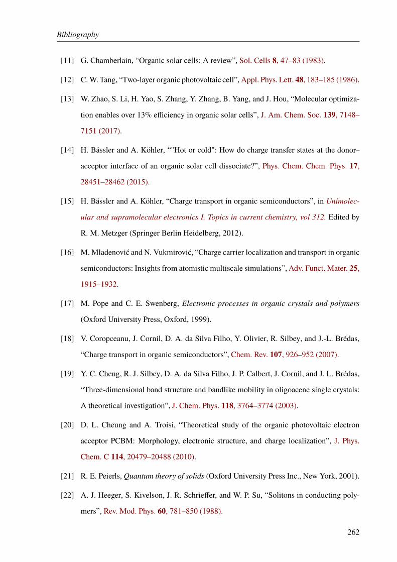
Bibliography
[11] G. Chamberlain, “Organic solar cells: A review”, Sol. Cells 8, 47–83 (1983).
[12] C. W. Tang, “Two-layer organic photovoltaic cell”, Appl. Phys. Lett. 48, 183–185 (1986).
[13] W. Zhao, S. Li, H. Yao, S. Zhang, Y. Zhang, B. Yang, and J. Hou, “Molecular optimiza-
tion enables over 13% efficiency in organic solar cells”, J. Am. Chem. Soc. 139, 7148–
7151 (2017).
[14] H. Bässler and A. Köhler, “"Hot or cold": How do charge transfer states at the donor–
acceptor interface of an organic solar cell dissociate?”, Phys. Chem. Chem. Phys. 17,
28451–28462 (2015).
[15] H. Bässler and A. Köhler, “Charge transport in organic semiconductors”, in Unimolec-
ular and supramolecular electronics I. Topics in current chemistry, vol 312. Edited by
R. M. Metzger (Springer Berlin Heidelberg, 2012).
[16] M. Mladenović and N. Vukmirović, “Charge carrier localization and transport in organic
semiconductors: Insights from atomistic multiscale simulations”, Adv. Funct. Mater. 25,
1915–1932.
[17] M. Pope and C. E. Swenberg, Electronic processes in organic crystals and polymers
(Oxford University Press, Oxford, 1999).
[18] V. Coropceanu, J. Cornil, D. A. da Silva Filho, Y. Olivier, R. Silbey, and J.-L. Brédas,
“Charge transport in organic semiconductors”, Chem. Rev. 107, 926–952 (2007).
[19] Y. C. Cheng, R. J. Silbey, D. A. da Silva Filho, J. P. Calbert, J. Cornil, and J. L. Brédas,
“Three-dimensional band structure and bandlike mobility in oligoacene single crystals:
A theoretical investigation”, J. Chem. Phys. 118, 3764–3774 (2003).
[20] D. L. Cheung and A. Troisi, “Theoretical study of the organic photovoltaic electron
acceptor PCBM: Morphology, electronic structure, and charge localization”, J. Phys.
Chem. C 114, 20479–20488 (2010).
[21] R. E. Peierls, Quantum theory of solids (Oxford University Press Inc., New York, 2001).
[22] A. J. Heeger, S. Kivelson, J. R. Schrieffer, and W. P. Su, “Solitons in conducting poly-
mers”, Rev. Mod. Phys. 60, 781–850 (1988).
262

Bibliography
[23] M. Mladenović and N. Vukmirović, “Effects of thermal disorder on the electronic prop-
erties of ordered polymers”, Phys. Chem. Chem. Phys. 16, 25950–25958 (2014).
[24] A. Maillard and A. Rochefort, “Structural and electronic properties of poly(3-hexylthiophene)
π-stacked crystals”, Phys. Rev. B 79, 115207 (2009).
[25] J. E. Northrup, “Atomic and electronic structure of polymer organic semiconductors:
P3HT, PQT, and PBTTT”, Phys. Rev. B 76, 245202 (2007).
[26] R. A. Street, S. A. Hawks, P. P. Khlyabich, G. Li, B. J. Schwartz, B. C. Thompson, and
Y. Yang, “Electronic structure and transition energies in polymer–fullerene bulk hetero-
junctions”, J. Phys. Chem. C 118, 21873–21883 (2014).
[27] I.-W. Hwang, C. Soci, D. Moses, Z. Zhu, D. Waller, R. Gaudiana, C. Brabec, and A.
Heeger, “Ultrafast electron transfer and decay dynamics in a small band gap bulk het-
erojunction material”, Adv. Mater. 19, 2307–2312 (2007).
[28] J.-L. Brédas, J. E. Norton, J. Cornil, and V. Coropceanu, “Molecular understanding of
organic solar cells: The challenges”, Acc. Chem. Res. 42, 1691–1699 (2009).
[29] G. Yu, J. Gao, J. C. Hummelen, F. Wudl, and A. J. Heeger, “Polymer photovoltaic cells:
Enhanced efficiencies via a network of internal donor–acceptor heterojunctions”, Science
270, 1789–1791 (1995).
[30] N. S. Sariciftci, L. Smilowitz, A. J. Heeger, and F. Wudl, “Photoinduced electron transfer
from a conducting polymer to buckminsterfullerene”, Science 258, 1474–1476 (1992).
[31] T. M. Clarke and J. R. Durrant, “Charge photogeneration in organic solar cells”, Chem.
Rev. 110, 6736–6767 (2010).
[32] Y. Tamai, H. Ohkita, H. Benten, and S. Ito, “Exciton diffusion in conjugated polymers:
From fundamental understanding to improvement in photovoltaic conversion efficiency”,
J. Phys. Chem. Lett. 6, 3417–3428 (2015).
[33] S. R. Cowan, N. Banerji, W. L. Leong, and A. J. Heeger, “Charge formation, recombina-
tion, and sweep-out dynamics in organic solar cells”, Adv. Funct. Mater. 22, 1116–1128
(2012).
263

Bibliography
[34] C. Deibel, T. Strobel, and V. Dyakonov, “Role of the charge transfer state in organic
donor–acceptor solar cells”, Adv. Mater. 22, 4097–4111.
[35] C. J. Brabec, G. Zerza, G. Cerullo, S. D. Silvestri, S. Luzzati, J. C. Hummelen, and S.
Sariciftci, “Tracing photoinduced electron transfer process in conjugated polymer/fullerene
bulk heterojunctions in real time”, Chem. Phys. Lett. 340, 232–236 (2001).
[36] G. Grancini, M. Maiuri, D. Fazzi, A. Petrozza, H.-J. Egelhaaf, D. Brida, G. Cerullo,
and G. Lanzani, “Hot exciton dissociation in polymer solar cells”, Nat. Mater. 12, 29–33
(2013).
[37] A. E. Jailaubekov, A. P. Willard, J. R. Tritsch, W.-L. Chan, N. Sai, R. Gearba, L. G.
Kaake, K. J. Williams, K. Leung, P. J. Rossky, and X.-Y. Zhu, “Hot charge-transfer ex-
citons set the time limit for charge separation at donor/acceptor interfaces in organic
photovoltaics”, Nat. Mater. 12, 66–73 (2013).
[38] S. Gélinas, A. Rao, A. Kumar, S. L. Smith, A. W. Chin, J. Clark, T. S. van der Poll, G. C.
Bazan, and R. H. Friend, “Ultrafast long-range charge separation in organic semiconduc-
tor photovoltaic diodes”, Science 343, 512–516 (2014).
[39] A. A. Paraecattil and N. Banerji, “Charge separation pathways in a highly efficient poly-
mer: fullerene solar cell material”, J. Am. Chem. Soc. 136, 1472–1482 (2014).
[40] F. Gao and O. Inganäs, “Charge generation in polymer–fullerene bulk-heterojunction
solar cells”, Phys. Chem. Chem. Phys. 16, 20291–20304 (2014).
[41] O. Ostroverkhova, “Organic optoelectronic materials: Mechanisms and applications”,
Chem. Rev. 116, 13279–13412 (2016).
[42] C. S. Ponseca, P. Chábera, J. Uhlig, P. Persson, and V. Sundström, “Ultrafast electron
dynamics in solar energy conversion”, Chem. Rev. 117, 10940–11024 (2017).
[43] S. Few, J. M. Frost, and J. Nelson, “Models of charge pair generation in organic solar
cells”, Phys. Chem. Chem. Phys. 17, 2311–2325 (2015).
264

Bibliography
[44] A. J. Heeger, “Nature of the primary photo-excitations in poly (arylene-vinylenes): Bound
neutral excitons or charged polaron pairs”, in Primary photoexcitations in conjugated
polymers: Molecular exciton versus semiconductor band model, edited by N. S. Sari-
ciftci (World Scientific, 1998).
[45] H. Bässler, “Excitons in conjugated polymers”, in Primary photoexcitations in conju-
gated polymers: Molecular exciton versus semiconductor band model, edited by N. S.
Sariciftci (World Scientific, 1998).
[46] N. Banerji, S. Cowan, M. Leclerc, E. Vauthey, and A. J. Heeger, “Exciton formation,
relaxation, and decay in PCDTBT”, J. Am. Chem. Soc. 132, 17459–17470 (2010).
[47] N. Banerji, S. Cowan, E. Vauthey, and A. J. Heeger, “Ultrafast relaxation of the poly(3-
hexylthiophene) emission spectrum”, J. Phys. Chem. C 115, 9726–9739 (2011).
[48] A. A. Bakulin, A. Rao, V. G. Pavelyev, P. H. M. van Loosdrecht, M. S. Pshenichnikov,
D. Niedzialek, J. Cornil, D. Beljonne, and R. H. Friend, “The role of driving energy and
delocalized states for charge separation in organic semiconductors”, Science 335, 1340–
1344 (2012).
[49] A. Troisi, “How quasi-free holes and electrons are generated in organic photovoltaic
interfaces”, Faraday Discuss. 163, 377–392 (2013).
[50] H. Vázquez and A. Troisi, “Calculation of rates of exciton dissociation into hot charge-
transfer states in model organic photovoltaic interfaces”, Phys. Rev. B 88, 205304 (2013).
[51] B. M. Savoie, A. Rao, A. A. Bakulin, S. Gelinas, B. Movaghar, R. H. Friend, T. J.
Marks, and M. A. Ratner, “Unequal partnership: Asymmetric roles of polymeric donor
and fullerene acceptor in generating free charge”, J. Am. Chem. Soc. 136, 2876–2884
(2014).
[52] Z. Sun and S. Stafström, “Dynamics of charge separation at an organic donor-acceptor
interface”, Phys. Rev. B 90, 115420 (2014).
[53] G. Nan, X. Zhang, and G. Lu, “Do "hot" charge-transfer excitons promote free carrier
generation in organic photovoltaics?”, J. Phys. Chem. C 119, 15028–15035 (2015).
265

Bibliography
[54] H. Tamura, I. Burghardt, and M. Tsukada, “Exciton dissociation at thiophene/fullerene
interfaces: The electronic structures and quantum dynamics”, J. Phys. Chem. C 115,
10205–10210 (2011).
[55] H. Tamura, R. Martinazzo, M. Ruckenbauer, and I. Burghardt, “Quantum dynamics of
ultrafast charge transfer at an oligothiophene-fullerene heterojunction”, J. Chem. Phys.
137, 22A540 (2012).
[56] H. Tamura and I. Burghardt, “Ultrafast charge separation in organic photovoltaics en-
hanced by charge delocalization and vibronically hot exciton dissociation”, J. Am. Chem.
Soc. 135, 16364–16367 (2013).
[57] E. R. Bittner and C. Silva, “Noise-induced quantum coherence drives photo-carrier gen-
eration dynamics at polymeric semiconductor heterojunctions”, Nat. Commun. 5, 3119
(2014).
[58] S. L. Smith and A. W. Chin, “Phonon-assisted ultrafast charge separation in the PCBM
band structure”, Phys. Rev. B 91, 201302 (2015).
[59] M. Huix-Rotllant, H. Tamura, and I. Burghardt, “Concurrent effects of delocalization
and internal conversion tune charge separation at regioregular polythiophene–fullerene
heterojunctions”, J. Phys. Chem. Lett. 6, 1702–1708 (2015).
[60] J. Lee, K. Vandewal, S. R. Yost, M. E. Bahlke, L. Goris, M. A. Baldo, J. V. Manca, and
T. V. Voorhis, “Charge transfer state versus hot exciton dissociation in polymer–fullerene
blended solar cells”, J. Am. Chem. Soc. 132, 11878–11880 (2010).
[61] K. Vandewal, S. Albrecht, E. T. Hoke, K. R. Graham, J. Widmer, J. D. Douglas, M.
Schubert, W. R. Mateker, J. T. Bloking, G. F. Burkhard, A. Sellinger, J. M. J. Fréchet,
A. Amassian, M. K. Riede, M. D. McGehee, D. Neher, and A. Salleo, “Efficient charge
generation by relaxed charge-transfer states at organic interfaces”, Nat. Mater. 13, 63–68
(2014).
[62] D. A. Vithanage, A. Devižis, V. Abramavičius, Y. Infahsaeng, D. Abramavičius, R. C. I.
MacKenzie, P. E. Keivanidis, A. Yartsev, D. Hertel, J. Nelson, V. Sundström, and V.
266

Bibliography
Gulbinas, “Visualizing charge separation in bulk heterojunction organic solar cells”, Nat.
Commun. 4, 2334 (2013).
[63] A. Devižis, J. De Jonghe-Risse, R. Hany, F. Nüesch, S. Jenatsch, V. Gulbinas, and J.-E.
Moser, “Dissociation of charge transfer states and carrier separation in bilayer organic
solar cells: A time-resolved electroabsorption spectroscopy study”, J. Am. Chem. Soc.
137, 8192–8198 (2015).
[64] L. Onsager, “Initial recombination of ions”, Phys. Rev. 54, 554–557 (1938).
[65] C. L. Braun, “Electric field assisted dissociation of charge transfer states as a mechanism
of photocarrier production”, J. Chem. Phys. 80, 4157–4161 (1984).
[66] C. Schwarz, S. Tscheuschner, J. Frisch, S. Winkler, N. Koch, H. Bässler, and A. Köhler,
“Role of the effective mass and interfacial dipoles on exciton dissociation in organic
donor-acceptor solar cells”, Phys. Rev. B 87, 155205 (2013).
[67] S. D. Baranovskii, M. Wiemer, A. V. Nenashev, F. Jansson, and F. Gebhard, “Calculating
the efficiency of exciton dissociation at the interface between a conjugated polymer and
an electron acceptor”, J. Phys. Chem. Lett. 3, 1214–1221 (2012).
[68] S. Athanasopoulos, S. Tscheuschner, H. Bässler, and A. Köhler, “Efficient charge sepa-
ration of cold charge-transfer states in organic solar cells through incoherent hopping”,
J. Phys. Chem. Lett. 8, 2093–2098 (2017).
[69] T. M. Burke and M. D. McGehee, “How high local charge carrier mobility and an energy
cascade in a three-phase bulk heterojunction enable >90% quantum efficiency”, Adv.
Mater. 26, 1923–1928 (2014).
[70] H. van Eersel, R. A. J. Janssen, and M. Kemerink, “Mechanism for efficient photoinduced
charge separation at disordered organic heterointerfaces”, Adv. Funct. Mater. 22, 2700–
2708 (2012).
[71] V. M. Axt and S. Mukamel, “Nonlinear optics of semiconductor and molecular nanos-
tructures: A common perspective”, Rev. Mod. Phys. 70, 145–174 (1998).
267

Bibliography
[72] F. Rossi and T. Kuhn, “Theory of ultrafast phenomena in photoexcited semiconductors”,
Rev. Mod. Phys. 74, 895–950 (2002).
[73] V. M. Axt and T. Kuhn, “Femtosecond spectroscopy in semiconductors: A key to coher-
ences, correlations and quantum kinetics”, Rep. Prog. Phys. 67, 433 (2004).
[74] A. Stahl and I. Balslev, Electrodynamics of the semiconductor band edge (Springer-
Verlag Berlin Heidelberg, 1987).
[75] T. Meier, P. Thomas, and S. Koch, Coherent semiconductor optics (Springer-Verlag Berlin
Heidelberg, 2007).
[76] E. Hanamura and H. Haug, “Condensation effects of excitons”, Phys. Rep. 33, 209–284
(1977).
[77] W. Barford, Electronic and optical properties of conjugated polymers (Oxford University
Press Inc., New York, 2005).
[78] S. Abe, J. Yu, and W. P. Su, “Singlet and triplet excitons in conjugated polymers”, Phys.
Rev. B 45, 8264–8271 (1992).
[79] D. Beljonne, Z. Shuai, G. Pourtois, and J. L. Brédas, “Spin–orbit coupling and intersys-
tem crossing in conjugated polymers: A configuration interaction description”, J. Phys.
Chem. A 105, 3899–3907 (2001).
[80] A. Köhler and H. Bässler, “Triplet states in organic semiconductors”, Mater. Sci. Eng.,
R 66, 71–109 (2009).
[81] G. H. Wannier, “The structure of electronic excitation levels in insulating crystals”, Phys.
Rev. 52, 191–197 (1937).
[82] J. Frenkel, “On the transformation of light into heat in solids. I”, Phys. Rev. 37, 17–44
(1931).
[83] J. Frenkel, “On the transformation of light into heat in solids. II”, Phys. Rev. 37, 1276–
1294 (1931).
[84] H. Haken, Quantum field theory of solids: An introduction (North-Holland Publishing
Company, 1976).
268

Bibliography
[85] M. Combescot and W. Pogosov, “Microscopic derivation of Frenkel excitons in second
quantization”, Phys. Rev. B 77, 085206 (2008).
[86] R. S. Knox, Theory of excitons (Academic Press, 1963).
[87] W. Huhn and A. Stahl, “Self-consistent field theory applied to the semiconductor band
edge”, Phys. Status Solidi B 124, 167–177 (1984).
[88] T. Förster, “Delocalized excitation and excitation transfer”, in Bulletin No. 18, Division
of biology and medicine (U. S. Atomic Energy Commission, 1965).
[89] V. Janković and N. Vukmirović, “Dynamics of exciton formation and relaxation in pho-
toexcited semiconductors”, Phys. Rev. B 92, 235208 (2015).
[90] T. Kuhn, “Density matrix theory of coherent ultrafast dynamics”, in Theory of transport
properties of semiconductor nanostructures, edited by E. Schöll (Chapman and Hall,
London, 1998).
[91] F. Rossi, Theory of semiconductor quantum devices: Microscopic modeling and simula-
tion strategies (Springer-Verlag Berlin Heidelberg, 2011).
[92] L. P. Kadanoff and G. Baym, Quantum statistical mechanics (Benjamin, New York,
1962).
[93] L. V. Keldysh, “Diagram technique for nonequilibrium processes”, Sov. Phys. JETP 20,
1018–1026 (1965).
[94] H. Haug and A.-P. Jauho, Quantum kinetics in transport and optics of semiconductors
(Springer, Berlin, 1996).
[95] A. V. Kuznetsov, “Interaction of ultrashort light pulses with semiconductors: Effec-
tive Bloch equations with relaxation and memory effects”, Phys. Rev. B 44, 8721–8744
(1991).
[96] H. Haug, “Interband quantum kinetics with LO-phonon scattering in a laser-pulse-excited
semiconductor I. Theory”, Phys. Status Solidi B 173, 139–148 (1992).
269
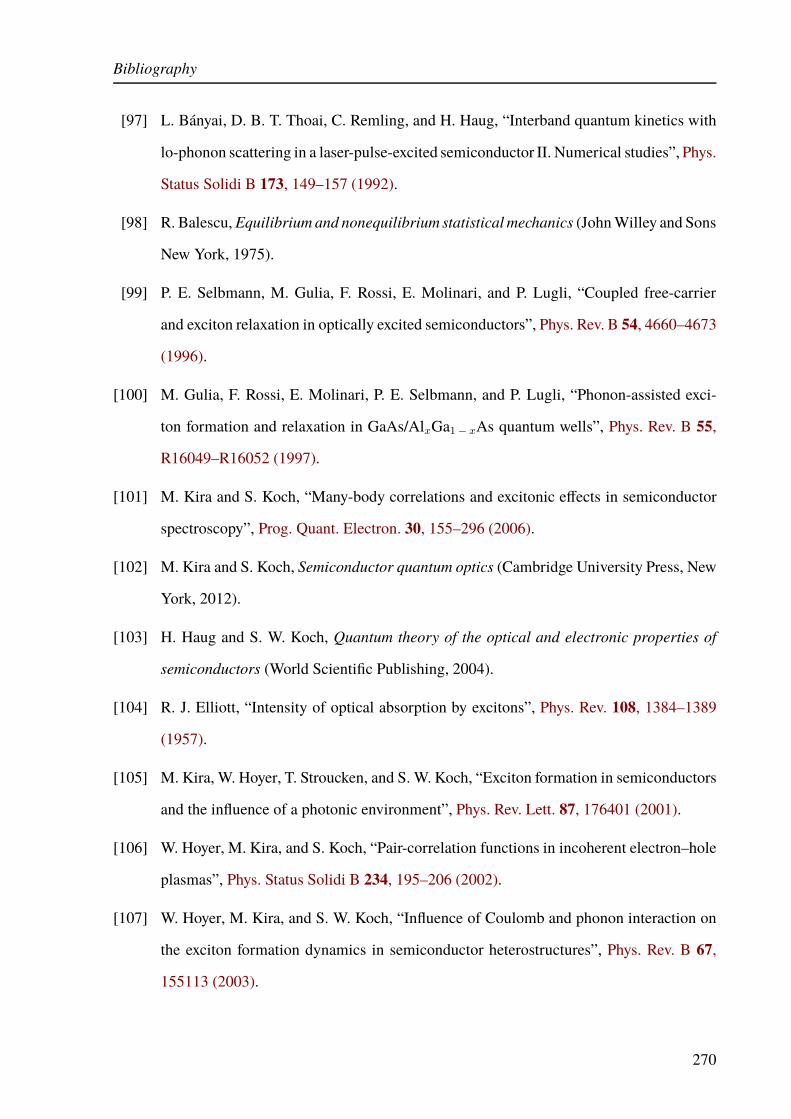
Bibliography
[97] L. Bányai, D. B. T. Thoai, C. Remling, and H. Haug, “Interband quantum kinetics with
lo-phonon scattering in a laser-pulse-excited semiconductor II. Numerical studies”, Phys.
Status Solidi B 173, 149–157 (1992).
[98] R. Balescu, Equilibrium and nonequilibrium statistical mechanics (John Willey and Sons
New York, 1975).
[99] P. E. Selbmann, M. Gulia, F. Rossi, E. Molinari, and P. Lugli, “Coupled free-carrier
and exciton relaxation in optically excited semiconductors”, Phys. Rev. B 54, 4660–4673
(1996).
[100] M. Gulia, F. Rossi, E. Molinari, P. E. Selbmann, and P. Lugli, “Phonon-assisted exci-
ton formation and relaxation in GaAs/AlxGa1− xAs quantum wells”, Phys. Rev. B 55,
R16049–R16052 (1997).
[101] M. Kira and S. Koch, “Many-body correlations and excitonic effects in semiconductor
spectroscopy”, Prog. Quant. Electron. 30, 155–296 (2006).
[102] M. Kira and S. Koch, Semiconductor quantum optics (Cambridge University Press, New
York, 2012).
[103] H. Haug and S. W. Koch, Quantum theory of the optical and electronic properties of
semiconductors (World Scientific Publishing, 2004).
[104] R. J. Elliott, “Intensity of optical absorption by excitons”, Phys. Rev. 108, 1384–1389
(1957).
[105] M. Kira, W. Hoyer, T. Stroucken, and S. W. Koch, “Exciton formation in semiconductors
and the influence of a photonic environment”, Phys. Rev. Lett. 87, 176401 (2001).
[106] W. Hoyer, M. Kira, and S. Koch, “Pair-correlation functions in incoherent electron–hole
plasmas”, Phys. Status Solidi B 234, 195–206 (2002).
[107] W. Hoyer, M. Kira, and S. W. Koch, “Influence of Coulomb and phonon interaction on
the exciton formation dynamics in semiconductor heterostructures”, Phys. Rev. B 67,
155113 (2003).
270

Bibliography
[108] V. Axt and A. Stahl, “A dynamics-controlled truncation scheme for the hierarchy of den-
sity matrices in semiconductor optics”, Z. Phys. B 93, 195–204 (1994).
[109] V. Axt and A. Stahl, “The role of the biexciton in a dynamic density matrix theory of the
semiconductor band edge”, Z. Phys. B 93, 205–211 (1994).
[110] K. Victor, V. M. Axt, and A. Stahl, “Hierarchy of density matrices in coherent semicon-
ductor optics”, Phys. Rev. B 51, 14164–14175 (1995).
[111] V. M. Axt, K. Victor, and A. Stahl, “Influence of a phonon bath on the hierarchy of
electronic densities in an optically excited semiconductor”, Phys. Rev. B 53, 7244–7258
(1996).
[112] M. Lindberg, Y. Z. Hu, R. Binder, and S. W. Koch, “χ(3) formalism in optically excited
semiconductors and its applications in four-wave-mixing spectroscopy”, Phys. Rev. B 50,
18060–18072 (1994).
[113] J. Shah, Ultrafast spectroscopy of semiconductors and semiconductor nanostructures
(Springer-Verlag Berlin Heidelberg, 1999).
[114] J. J. Sakurai and J. Napolitano, Modern quantum mechanics, second edition (Addison-
Wesley, 2011).
[115] K. Siantidis, V. M. Axt, and T. Kuhn, “Dynamics of exciton formation for near band-gap
excitations”, Phys. Rev. B 65, 035303 (2001).
[116] K Siantidis, T Wolterink, V. Axt, and T Kuhn, “Formation of excitons from correlated
electron–hole pairs”, Physica B 314, 220–223 (2002).
[117] K Siantidis, V. Axt, J Wühr, and T Kuhn, “Theory of exciton formation and relaxation
in quantum wires”, Phys. Status Solidi A 190, 743–747 (2002).
[118] T. Kuhn and F. Rossi, “Monte Carlo simulation of ultrafast processes in photoexcited
semiconductors: Coherent and incoherent dynamics”, Phys. Rev. B 46, 7496–7514 (1992).
[119] J. Schilp, T. Kuhn, and G. Mahler, “Electron-phonon quantum kinetics in pulse-excited
semiconductors: Memory and renormalization effects”, Phys. Rev. B 50, 5435–5447
(1994).
271

Bibliography
[120] J. Schilp, T. Kuhn, and G. Mahler, “Quantum kinetics of the coupled carrier-phonon
system in photoexcited semiconductors”, Phys. Status Solidi B 188, 417–424 (1995).
[121] V. Chernyak and S. Mukamel, “Third-order optical response of intermediate excitons
with fractional nonlinear statistics”, J. Opt. Soc. Am. B 13, 1302–1307 (1996).
[122] W. M. Zhang, T. Meier, V. Chernyak, and S. Mukamel, “Intraband terahertz emission
from coupled semiconductor quantum wells: A model study using the exciton represen-
tation”, Phys. Rev. B 60, 2599–2609 (1999).
[123] C. Haik, T. Seiji, and T. Fumio, “Ultrafast fluorescence upconversion technique and its
applications to proteins”, FEBS J. 282, 3003–3015.
[124] M. N. Kobrak and E. R. Bittner, “Quantum molecular dynamics study of polaron recom-
bination in conjugated polymers”, Phys. Rev. B 62, 11473–11486 (2000).
[125] K. Tandon, S. Ramasesha, and S. Mazumdar, “Electron correlation effects in electron-
hole recombination in organic light-emitting diodes”, Phys. Rev. B 67, 045109 (2003).
[126] N. Vukmirović, C. Bruder, and V. M. Stojanović, “Electron-phonon coupling in crys-
talline organic semiconductors: Microscopic evidence for nonpolaronic charge carriers”,
Phys. Rev. Lett. 109, 126407 (2012).
[127] S. D. Dimitrov, B. C. Schroeder, C. B. Nielsen, H. Bronstein, Z. Fei, I. McCulloch, M.
Heeney, and J. R. Durrant, “Singlet exciton lifetimes in conjugated polymer films for
organic solar cells”, Polymers 8, 14 (2016).
[128] M. Levinshtein, S. Rumyantsev, and M. Shur, Handbook series on semiconductor pa-
rameters, volume 1 (World Scientific, 1996).
[129] Y.-C. Cheng and R. J. Silbey, “A unified theory for charge-carrier transport in organic
crystals”, J. Chem. Phys. 128, 114713 (2008).
[130] P. Cudazzo, F. Sottile, A. Rubio, and M. Gatti, “Exciton dispersion in molecular solids”,
J. Phys.: Condens. Matter 27, 113204 (2015).
272

Bibliography
[131] A. Troisi and G. Orlandi, “Charge-transport regime of crystalline organic semiconduc-
tors: Diffusion limited by thermal off-diagonal electronic disorder”, Phys. Rev. Lett. 96,
086601 (2006).
[132] K. Fujii, S. Kera, M. Oiwa, K. K. Okudaira, K. Sakamoto, and N. Ueno, “Influence of
intramolecular vibrations in charge redistribution at the pentacene–graphite interface”,
Surf. Sci. 601, 3765–3768 (2007).
[133] W. H. Press, S. A. Teukolsky, W. T. Vetterling, and B. P. Flannery, Numerical recipes in
C: The art of scientific computing, second edition (Cambridge University Press, 1992).
[134] V. Janković and N. Vukmirović, “Origin of space-separated charges in photoexcited or-
ganic heterojunctions on ultrafast time scales”, Phys. Rev. B 95, 075308 (2017).
[135] C. Silva, “Some like it hot”, Nat. Mater. 12, 5–6 (2012).
[136] I.-W. Hwang, D. Moses, and A. J. Heeger, “Photoinduced carrier generation in P3HT/PCBM
bulk heterojunction materials”, J. Phys. Chem. C 112, 4350–4354 (2008).
[137] T. Liu and A. Troisi, “What makes fullerene acceptors special as electron acceptors in
organic solar cells and how to replace them”, Adv. Mater. 25, 1038–1041 (2013).
[138] S. L. Smith and A. W. Chin, “Ultrafast charge separation and nongeminate electron–hole
recombination in organic photovoltaics”, Phys. Chem. Chem. Phys. 16, 20305–20309
(2014).
[139] S. M. Falke, C. A. Rozzi, D. Brida, M. Maiuri, M. Amato, E. Sommer, A. De Sio, A.
Rubio, G. Cerullo, E. Molinari, and C. Lienau, “Coherent ultrafast charge transfer in an
organic photovoltaic blend”, Science 344, 1001–1005 (2014).
[140] H. Tamura, J. G. S. Ramon, E. R. Bittner, and I. Burghardt, “Phonon-driven ultrafast
exciton dissociation at donor-acceptor polymer heterojunctions”, Phys. Rev. Lett. 100,
107402 (2008).
[141] M. H. Lee, J. Aragó, and A. Troisi, “Charge dynamics in organic photovoltaic materials:
Interplay between quantum diffusion and quantum relaxation”, J. Phys. Chem. C 119,
14989–14998 (2015).
273

Bibliography
[142] S. Bera, N. Gheeraert, S. Fratini, S. Ciuchi, and S. Florens, “Impact of quantized vibra-
tions on the efficiency of interfacial charge separation in photovoltaic devices”, Phys.
Rev. B 91, 041107 (2015).
[143] H. Ma and A. Troisi, “Direct optical generation of long-range charge-transfer states in
organic photovoltaics”, Adv. Mater. 26, 6163–6167 (2014).
[144] G. D’Avino, L. Muccioli, Y. Olivier, and D. Beljonne, “Charge separation and recombi-
nation at polymer–fullerene heterojunctions: Delocalization and hybridization effects”,
J. Phys. Chem. Lett. 7, 536–540 (2016).
[145] D. Mühlbacher, M. Scharber, M. Morana, Z. Zhu, D. Waller, R. Gaudiana, and C. Brabec,
“High photovoltaic performance of a low-bandgap polymer”, Adv. Mater. 18, 2884–2889
(2006).
[146] H. Tamura and M. Tsukada, “Role of intermolecular charge delocalization on electron
transport in fullerene aggregates”, Phys. Rev. B 85, 054301 (2012).
[147] P. Giannozzi and et al., “QUANTUM ESPRESSO: a modular and open-source software
project for quantum simulations of materials”, J. Phys.: Condens. Matter 21, 395502
(2009).
[148] Y. Kanai and J. C. Grossman, “Insights on interfacial charge transfer across P3HT/fullerene
photovoltaic heterojunction from ab initio calculations”, Nano Lett. 7, 1967–1972 (2007).
[149] E. R. Bittner and J. G. S. Ramon, “Exciton and charge-transfer dynamics in polymer
semiconductors”, in Quantum dynamics of complex molecular systems, edited by D. A.
Micha and I. Burghardt (Springer-Verlag, Berlin Heidelberg, 2007).
[150] A. Lücke, F. Ortmann, M. Panhans, S. Sanna, E. Rauls, U. Gerstmann, and W. G. Schmidt,
“Temperature-dependent hole mobility and its limit in crystal-phase P3HT calculated
from first principles”, J. Phys. Chem. B 120, 5572–5580 (2016).
[151] N. Vukmirović and L.-W. Wang, “Charge carrier motion in disordered conjugated poly-
mers: A multiscale ab initio study”, Nano Lett. 9, 3996–4000 (2009).
274
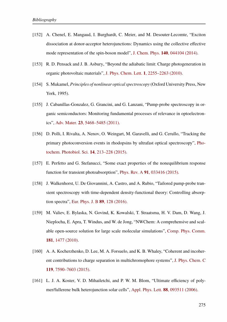
Bibliography
[152] A. Chenel, E. Mangaud, I. Burghardt, C. Meier, and M. Desouter-Lecomte, “Exciton
dissociation at donor-acceptor heterojunctions: Dynamics using the collective effective
mode representation of the spin-boson model”, J. Chem. Phys. 140, 044104 (2014).
[153] R. D. Pensack and J. B. Asbury, “Beyond the adiabatic limit: Charge photogeneration in
organic photovoltaic materials”, J. Phys. Chem. Lett. 1, 2255–2263 (2010).
[154] S. Mukamel, Principles of nonlinear optical spectroscopy (Oxford University Press, New
York, 1995).
[155] J. Cabanillas-Gonzalez, G. Grancini, and G. Lanzani, “Pump-probe spectroscopy in or-
ganic semiconductors: Monitoring fundamental processes of relevance in optoelectron-
ics”, Adv. Mater. 23, 5468–5485 (2011).
[156] D. Polli, I. Rivalta, A. Nenov, O. Weingart, M. Garavelli, and G. Cerullo, “Tracking the
primary photoconversion events in rhodopsins by ultrafast optical spectroscopy”, Pho-
tochem. Photobiol. Sci. 14, 213–228 (2015).
[157] E. Perfetto and G. Stefanucci, “Some exact properties of the nonequilibrium response
function for transient photoabsorption”, Phys. Rev. A 91, 033416 (2015).
[158] J. Walkenhorst, U. De Giovannini, A. Castro, and A. Rubio, “Tailored pump-probe tran-
sient spectroscopy with time-dependent density-functional theory: Controlling absorp-
tion spectra”, Eur. Phys. J. B 89, 128 (2016).
[159] M. Valiev, E. Bylaska, N. Govind, K. Kowalski, T. Straatsma, H. V. Dam, D. Wang, J.
Nieplocha, E. Apra, T. Windus, and W. de Jong, “NWChem: A comprehensive and scal-
able open-source solution for large scale molecular simulations”, Comp. Phys. Comm.
181, 1477 (2010).
[160] A. A. Kocherzhenko, D. Lee, M. A. Forsuelo, and K. B. Whaley, “Coherent and incoher-
ent contributions to charge separation in multichromophore systems”, J. Phys. Chem. C
119, 7590–7603 (2015).
[161] L. J. A. Koster, V. D. Mihailetchi, and P. W. M. Blom, “Ultimate efficiency of poly-
mer/fullerene bulk heterojunction solar cells”, Appl. Phys. Lett. 88, 093511 (2006).
275

Bibliography
[162] J. C. Tully, “Molecular dynamics with electronic transitions”, J. Chem. Phys. 93, 1061–
1071 (1990).
[163] L. Wang and O. V. Prezhdo, “A simple solution to the trivial crossing problem in surface
hopping”, J. Phys. Chem. Lett. 5, 713–719 (2014).
[164] K. Král and Z. Khás, “Electron self-energy in quantum dots”, Phys. Rev. B 57, R2061–
R2064 (1998).
[165] M. Menšík, J. Pfleger, and P. Toman, “Dynamics of photogenerated polarons and polaron
pairs in P3HT thin films”, Chem. Phys. Lett. 677, 87–91 (2017).
[166] V. Janković and N. Vukmirović, “Identification of ultrafast photophysical pathways in
photoexcited organic heterojunctions”, J. Phys. Chem. C 121, 19602–19618 (2017).
[167] S. Chun-Qi, W. Peng, S. Ying, L. Yan-Jun, Z. Wen-Hua, X. Fa-Qiang, Z. Jun-Fa, L. Guo-
Qiao, and L. Hong-Nian, “Electronic structure of PCBM”, Chin. Phys. B 21, 017102
(2012).
[168] J. Idé, D. Fazzi, M. Casalegno, S. V. Meille, and G. Raos, “Electron transport in crys-
talline PCBM-like fullerene derivatives: A comparative computational study”, J. Mater.
Chem. C 2, 7313–7325 (2014).
[169] H. Ma and A. Troisi, “Modulating the exciton dissociation rate by up to more than two
orders of magnitude by controlling the alignment of LUMO + 1 in organic photovoltaics”,
J. Phys. Chem. C 118, 27272–27280 (2014).
[170] Z. Li, X. Zhang, and G. Lu, “Electron structure and dynamics at poly(3-hexylthiophene)/fu-
llerene photovoltaic heterojunctions”, Appl. Phys. Lett. 98, 083303 (2011).
[171] T. Liu, D. L. Cheung, and A. Troisi, “Structural variability and dynamics of the P3HT/PCBM
interface and its effects on the electronic structure and the charge-transfer rates in solar
cells”, Phys. Chem. Chem. Phys. 13, 21461–21470 (2011).
[172] M. Fujii, W. Shin, T. Yasuda, and K. Yamashita, “Photon-absorbing charge-bridging
states in organic bulk heterojunctions consisting of diketopyrrolopyrrole derivatives and
PCBM”, Phys. Chem. Chem. Phys. 18, 9514–9523 (2016).
276

Bibliography
[173] Z. Sun and S. Stafström, “Dynamics of exciton dissociation in donor-acceptor polymer
heterojunctions”, J. Chem. Phys. 138, 164905 (2013).
[174] Y.-K. Lan and C.-I. Huang, “A theoretical study of the charge transfer behavior of the
highly regioregular poly-3-hexylthiophene in the ordered state”, J. Phys. Chem. B 112,
14857–14862 (2008).
[175] D. L. Cheung, D. P. McMahon, and A. Troisi, “Computational study of the structure and
charge-transfer parameters in low-molecular-mass P3HT”, J. Phys. Chem. B 113, 9393–
9401 (2009).
[176] R. S. Bhatta and M. Tsige, “Chain length and torsional dependence of exciton binding
energies in P3HT and PTB7 conjugated polymers: A first-principles study”, Polymer 55,
2667–2672 (2014).
[177] G. Grancini, D. Polli, D. Fazzi, J. Cabanillas-Gonzalez, G. Cerullo, and G. Lanzani,
“Transient absorption imaging of P3HT:PCBM photovoltaic blend: Evidence for inter-
facial charge transfer state”, J. Phys. Chem. Lett. 2, 1099–1105 (2011).
[178] Y. Yi, V. Coropceanu, and J.-L. Bredas, “A comparative theoretical study of exciton-
dissociation and charge-recombination processes in oligothiophene/fullerene and olig-
othiophene/perylenediimide complexes for organic solar cells”, J. Mater. Chem. 21, 1479–
1486 (2011).
[179] T. Liu and A. Troisi, “Absolute rate of charge separation and recombination in a molec-
ular model of the P3HT/PCBM interface”, J. Phys. Chem. C 115, 2406–2415 (2011).
[180] M. Schulze, M. Hänsel, and P. Tegeder, “Hot excitons increase the donor/acceptor charge
transfer yield”, J. Phys. Chem. C 118, 28527–28534 (2014).
[181] A. Grupp, P. Ehrenreich, J. Kalb, A. Budweg, L. Schmidt-Mende, and D. Brida, “Inco-
herent pathways of charge separation in organic and hybrid solar cells”, J. Phys. Chem.
Lett. 8, 4858–4864 (2017).
277
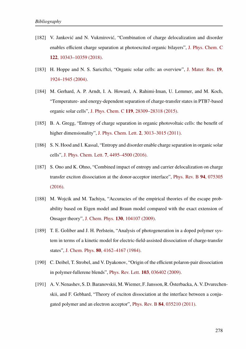
Bibliography
[182] V. Janković and N. Vukmirović, “Combination of charge delocalization and disorder
enables efficient charge separation at photoexcited organic bilayers”, J. Phys. Chem. C
122, 10343–10359 (2018).
[183] H. Hoppe and N. S. Sariciftci, “Organic solar cells: an overview”, J. Mater. Res. 19,
1924–1945 (2004).
[184] M. Gerhard, A. P. Arndt, I. A. Howard, A. Rahimi-Iman, U. Lemmer, and M. Koch,
“Temperature- and energy-dependent separation of charge-transfer states in PTB7-based
organic solar cells”, J. Phys. Chem. C 119, 28309–28318 (2015).
[185] B. A. Gregg, “Entropy of charge separation in organic photovoltaic cells: the benefit of
higher dimensionality”, J. Phys. Chem. Lett. 2, 3013–3015 (2011).
[186] S. N. Hood and I. Kassal, “Entropy and disorder enable charge separation in organic solar
cells”, J. Phys. Chem. Lett. 7, 4495–4500 (2016).
[187] S. Ono and K. Ohno, “Combined impact of entropy and carrier delocalization on charge
transfer exciton dissociation at the donor-acceptor interface”, Phys. Rev. B 94, 075305
(2016).
[188] M. Wojcik and M. Tachiya, “Accuracies of the empirical theories of the escape prob-
ability based on Eigen model and Braun model compared with the exact extension of
Onsager theory”, J. Chem. Phys. 130, 104107 (2009).
[189] T. E. Goliber and J. H. Perlstein, “Analysis of photogeneration in a doped polymer sys-
tem in terms of a kinetic model for electric-field-assisted dissociation of charge-transfer
states”, J. Chem. Phys. 80, 4162–4167 (1984).
[190] C. Deibel, T. Strobel, and V. Dyakonov, “Origin of the efficient polaron-pair dissociation
in polymer-fullerene blends”, Phys. Rev. Lett. 103, 036402 (2009).
[191] A. V. Nenashev, S. D. Baranovskii, M. Wiemer, F. Jansson, R. Österbacka, A. V. Dvurechen-
skii, and F. Gebhard, “Theory of exciton dissociation at the interface between a conju-
gated polymer and an electron acceptor”, Phys. Rev. B 84, 035210 (2011).
278
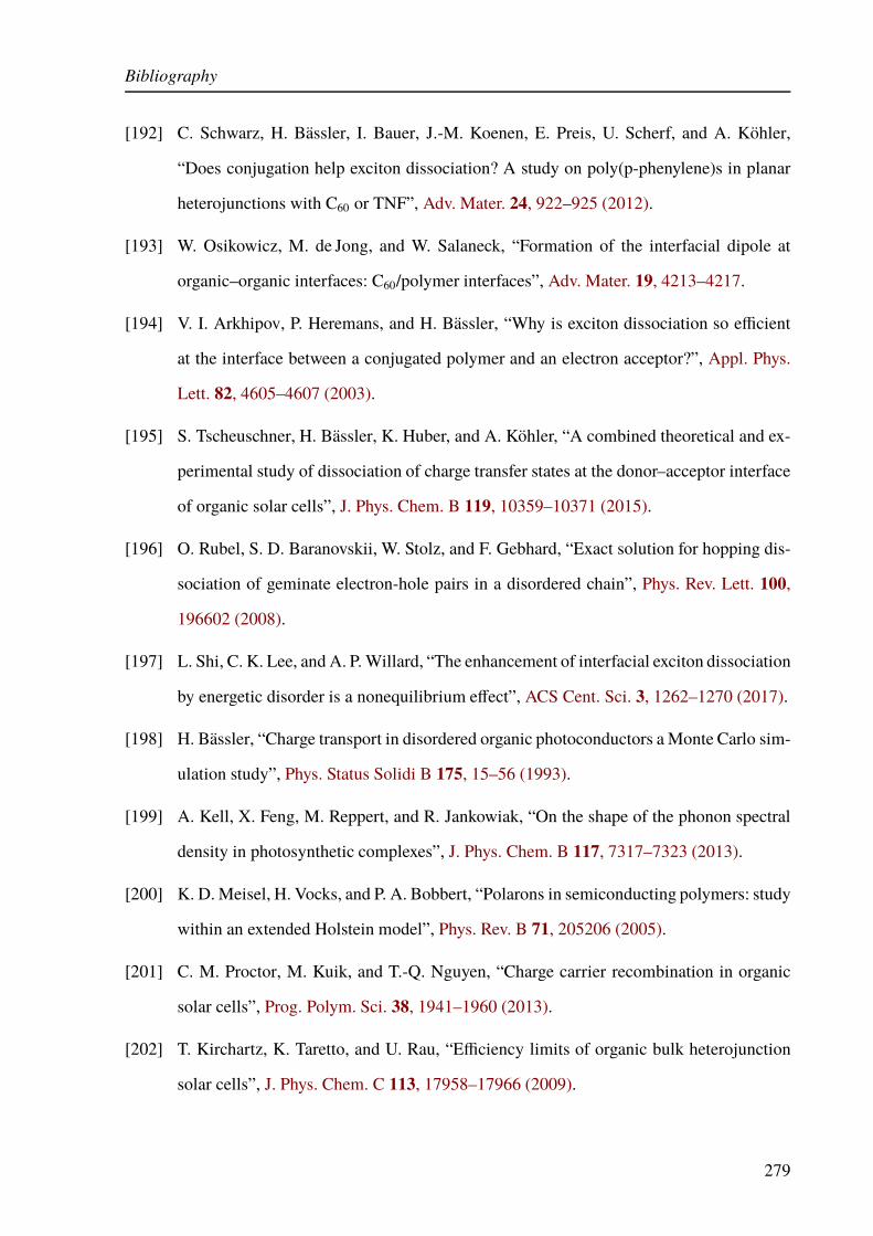
Bibliography
[192] C. Schwarz, H. Bässler, I. Bauer, J.-M. Koenen, E. Preis, U. Scherf, and A. Köhler,
“Does conjugation help exciton dissociation? A study on poly(p-phenylene)s in planar
heterojunctions with C60 or TNF”, Adv. Mater. 24, 922–925 (2012).
[193] W. Osikowicz, M. de Jong, and W. Salaneck, “Formation of the interfacial dipole at
organic–organic interfaces: C60/polymer interfaces”, Adv. Mater. 19, 4213–4217.
[194] V. I. Arkhipov, P. Heremans, and H. Bässler, “Why is exciton dissociation so efficient
at the interface between a conjugated polymer and an electron acceptor?”, Appl. Phys.
Lett. 82, 4605–4607 (2003).
[195] S. Tscheuschner, H. Bässler, K. Huber, and A. Köhler, “A combined theoretical and ex-
perimental study of dissociation of charge transfer states at the donor–acceptor interface
of organic solar cells”, J. Phys. Chem. B 119, 10359–10371 (2015).
[196] O. Rubel, S. D. Baranovskii, W. Stolz, and F. Gebhard, “Exact solution for hopping dis-
sociation of geminate electron-hole pairs in a disordered chain”, Phys. Rev. Lett. 100,
196602 (2008).
[197] L. Shi, C. K. Lee, and A. P. Willard, “The enhancement of interfacial exciton dissociation
by energetic disorder is a nonequilibrium effect”, ACS Cent. Sci. 3, 1262–1270 (2017).
[198] H. Bässler, “Charge transport in disordered organic photoconductors a Monte Carlo sim-
ulation study”, Phys. Status Solidi B 175, 15–56 (1993).
[199] A. Kell, X. Feng, M. Reppert, and R. Jankowiak, “On the shape of the phonon spectral
density in photosynthetic complexes”, J. Phys. Chem. B 117, 7317–7323 (2013).
[200] K. D. Meisel, H. Vocks, and P. A. Bobbert, “Polarons in semiconducting polymers: study
within an extended Holstein model”, Phys. Rev. B 71, 205206 (2005).
[201] C. M. Proctor, M. Kuik, and T.-Q. Nguyen, “Charge carrier recombination in organic
solar cells”, Prog. Polym. Sci. 38, 1941–1960 (2013).
[202] T. Kirchartz, K. Taretto, and U. Rau, “Efficiency limits of organic bulk heterojunction
solar cells”, J. Phys. Chem. C 113, 17958–17966 (2009).
279

Bibliography
[203] T. Offermans, S. C. J. Meskers, and R. A. J. Janssen, “Monte-Carlo simulations of gem-
inate electron-hole pair dissociation in a molecular heterojunction: A two-step dissocia-
tion mechanism”, Chem. Phys. 308, 125–133 (2005).
[204] A. P. Arndt, M. Gerhard, A. Quintilla, I. A. Howard, M. Koch, and U. Lemmer, “Time-
resolved charge-transfer state emission in organic solar cells: temperature and blend com-
position dependences of interfacial traps”, J. Phys. Chem. C 119, 13516–13523 (2015).
[205] J. H. Choi, K.-I. Son, T. Kim, K. Kim, K. Ohkubo, and S. Fukuzumi, “Thienyl-substituted
methanofullerene derivatives for organic photovoltaic cells”, J. Mater. Chem. 20, 475–
482 (2010).
[206] N. B. Taylor and I. Kassal, “Generalised Marcus theory for multi-molecular delocalised
charge transfer”, Chem. Sci. 9, 2942–2951 (2018).
[207] Y. Yan, L. Song, and Q. Shi, “Understanding the free energy barrier and multiple timescale
dynamics of charge separation in organic photovoltaic cells”, J. Chem. Phys. 148, 084109
(2018).
280

Veljko Janković
Curriculum Vitae
Veljko Janković was born on September 23, 1990 in Belgrade, Republic of Serbia. He acquired
elementary and high-school education in Belgrade.
In 2009, Veljko Janković enrolled on bachelor studies of physics at the Faculty of Physics, Uni-
versity of Belgrade, and completed them in 2013 with a GPA of 9.97/10.00. As one of the best
third-year students at the Faculty of Physics, in 2012 he was awarded Prof. Dr Ðorđe Živanović
prize. In 2013, he started master studies with specialization in condensed matter physics, and
finished them in June 2014 by defending the MSc thesis entitled Nonequilibrium Optical Con-
ductivity in Systems with Localized Electronic States. The thesis was done in the Scientific
Computing Laboratory of the Institute of Physics Belgrade under supervision of Dr Nenad Vuk-
mirović. In October 2014, the thesis was awarded Prof. Dr Ljubomir Ćirković prize for the best
MSc thesis defended at the Faculty of Physics during the academic year 2013/14.
In November 2014, Veljko Janković started his doctoral studies at the Faculty of Physics, Uni-
versity of Belgrade, with specialization in condensed matter physics. The research project was
entirely conducted in the Scientific Computing Laboratory of the Institute of Physics Belgrade
and was supervised by Dr Nenad Vukmirović. The project was focused on fundamental phys-
ical understanding of the light-to-charge conversion in organic solar cells. In the course of his
doctoral programme, Veljko Janković published four peer-reviewed research papers directly con-
nected to the topic of the thesis (papers 2–5) and one paper that is not connected to the topic of
the thesis (paper 1).
5. V. Janković and N. Vukmirović, “Combination of Charge Delocalization and Disorder
Enables Efficient Charge Separation at Photoexcited Organic Bilayers”, J. Phys. Chem.
C, 122, 10343–10359 (2018).
4. V. Janković and N. Vukmirović, “Identification of Ultrafast Photophysical Pathways in
Photoexcited Organic Heterojunctions”, J. Phys. Chem. C 121, 19602–19618 (2017).
3. V. Janković and N. Vukmirović, “Origin of Space-separated Charges in Photoexcited Or-
ganic Heterojunctions on Ultrafast Time Scales”, Phys. Rev. B 95, 075308 (2017).

2. V. Janković and N. Vukmirović, “Dynamics of Exciton Formation and Relaxation in Pho-
toexcited Semiconductors”, Phys. Rev. B 92, 235208 (2015).
1. V. Janković and N. Vukmirović, “Nonequilibrium Optical Conductivity in Materials with
Localized Electronic States”, Phys. Rev. B 90, 224201 (2014).
Since November 2014, Veljko Janković has participated in the National Project ON171017 Mod-
eling and Numerical Simulations of Complex Many-Particle Systems funded by the Ministry of
Education, Science, and Technological Development of the Republic of Serbia. From October
2013 to August 2015, he participated in the European Community FP7 Marie Curie Integration
Grant ELECTROMAT, whose head was Dr Nenad Vukmirović. Since 2015, he has participated
in the COST Action MP1406 MultiscaleSolar. Veljko Janković has also been involved in the
teaching process at the Faculty of Physics, University of Belgrade, as an external collaborator
at the Chair of Theoretical Mechanics, Electrodynamics, and Statistical Physics. During the
academic year 2013/14, he was a teaching assistant in Theoretical Mechanics (lecturer Prof. Dr
Sunčica Elezović-Hadžić). Since the academic year 2014/15, he has been a teaching assistant in
Quantum Statistical Physics (lecturers Doc. Dr Mihajlo Vanević and Prof. Dr Zoran Radović).
During the school year 2012/13, as well as from the school year 2015/16 to 2017/18, Veljko
Janković actively participated in the National Committee for High-School Physics Competitions
as one of the authors of problems proposed to the final-year high-school students. He was one of
the team leaders of the Serbian national team at The 5th Romanian Master of Physics (Bucharest,
Romania, February 2016), The 48th International Physics Olympiad (Jogjakarta, Indonesia, July
2017), as well as at The 49th International Physics Olympiad (Lisbon, Portugal, July 2018). He
is fluent in English and Italian languages.
During his doctoral programme, Veljko Janković had an opportunity to present the results of his
research in the following conferences and workshops:
8. (oral) V. Janković and N. Vukmirović, “Importance of Carrier Delocalization and Disorder
for Incoherent Charge Separation at Organic Bilayers”, E-MRS Spring Meeting 2018, 18–
22 June 2018, Strasbourg Convention Center, Strasbourg, France, oral contribution J12.7
(2018).

7. (poster) V. Janković and N. Vukmirović, “Origin of Space-Separated Charges in Pho-
toexcited Organic Heterojunctions on Subpicosecond Time Scales”, The 6th International
School and Conference on Photonics, 28 August–1 September 2017, Belgrade, Serbia,
Book of Abstracts, p. 164 (2017).
6. (poster) V. Janković and N. Vukmirović, “Origin of Space-Separated Charges in Photoex-
cited Organic Heterojunctions on Ultrafast Time Scales”, Workshop on Spectroscopy and
Dynamics of Photoinduced Electronic Excitations, International Center for Theoretical
Physics, Trieste, Italy, 8–12 May 2017.
5. (poster) V. Janković and N. Vukmirović, “Exciton Formation and Relaxation Dynamics
in Photoexcited Organic Semiconductors and Their Heterojunctions: Numerical Study”,
Gordon Research Conference Electronic Processes in Organic Materials, Barga (Lucca),
Italy, 5−10 June 2016, Poster Presentation 41 (2016).
4. (poster) V. Janković and N. Vukmirović, “Nonequilibrium Electrical Transport in Materi-
als with Localized Electronic States”, The 26th International Conference on Amorphous
and Nanocrystalline Semiconductors, Aachen, Germany, 13−18 September 2015, Book
of Abstracts, p. 72 (2015).
3. (poster) V. Janković and N. Vukmirović, “Nonequilibrium High-Frequency Conductivity
in Materials with Localized Electronic States”, The 19th Symposium on Condensed Mat-
ter Physics (SFKM), Belgrade, Serbia, 7−11 September 2015, Book of Abstracts, p. 88
(2015).
2. (poster) V. Janković and N. Vukmirović, “Nonequilibrium Terahertz Conductivity in Sys-
tems with Localized Electronic States”, EDISON 19, 29 June−2 July 2015, Salamanca,
Spain, Book of Abstracts, p. 125 (2015).
1. (poster) V. Janković and N. Vukmirović, “Nonequilibrium Terahertz Conductivity in Ma-
terials with Localized Electronic States”, Nanoscale Quantum Optics-Kick off Workshop,
9−10 April 2015, Belgrade, Serbia, Book of Abstracts, p. 55 (2015).