DOI: 10.1111/eufm.12137

ORIGINAL ARTICLE

Exchange traded funds and asset returncorrelations

Zhi Da | Sophie Shive

Mendoza College of Business, Universityof Notre Dame, Notre Dame,IN 46556Emails: sshive1@nd.edu; zda@nd.edu

Abstract

We provide novel evidence supporting the notion that

arbitrageurs can contribute to return comovement via

exchange trade funds (ETF) arbitrage. Using a large sample

of US equity ETF holdings, we document the link between

measures of ETF activity and return comovement at both the

fund and the stock levels, after controlling for a host of

variables and fixed effects and by exploiting the ‘disconti-nuity’ between stock indices. The effect is also stronger

among small and illiquid stocks. An examination of ETF

return autocorrelations and stock lagged beta provides

evidence for price reversal, suggesting that someETF-driven

return comovement may be excessive.

KEYWORDS

exchange-traded-fund, correlation, arbitrage

J EL CLAS S I F ICAT ION

G23, G12

Thanks to participants in the 2012 State of Indiana Finance Conference, 2013 China International Conference in Finance,2nd Luxembourg Asset Management Summit, 2014 American Finance Association Annual Meeting, and seminars atNanyang Technological University, National University of Singapore, Singapore Management University, University ofCincinnati, University of Illinois at Urbana-Champaign, University of Notre Dame, Vanderbilt University, Malcom Baker,Robert Battalio, Hendrik Bessembinder, Martijn Cremers, Ben Golez, Robin Greenwood, Bing Han, Paul Schultz, DavidSolomon, Mao Ye and Xiaoyan Zhang for helpful comments. This article has been previously circulated under the title‘When the bellwether dances to noise: Evidence from exchange-traded funds’. Errors are ours.

Eur Financ Manag. 2017;1–33. wileyonlinelibrary.com/journal/eufm © 2017 John Wiley & Sons, Ltd. | 1

1 | INTRODUCTION

Perhaps due to a half-century of encouragement from finance academics, investment assets areincreasingly indexed, but the implications for asset prices of large amounts of indexed investment are notwell understood. Citing evidence of mispricing and increased correlations among asset returns, Wurgler(2010) warns that over-indexing may result in contagion and mispricing risk. Exchange-traded funds(ETFs), baskets of equities traded on an exchange like stocks, are a growing asset class that has madeindexing cheaper and more convenient for many investors. US-based exchange-traded funds had US$ 1.7 trillion in assets under management by the end of 2013.1 Since these funds will by all measuresplay a large role in the future of saving and investing, it is important to understand if and how theywill affect prices, both in absolute and compared to traditional mutual funds and institutions.

Along with information, ETFs have a potential to transmit non-fundamental shocks. Demand forETFs results in price pressure, which is then transmitted to the underlying basket of shares asarbitrageurs simultaneously take opposite positions in the ETF and the underlying shares.2 As a result,stocks held by ETFs might comove more with each other than warranted by common exposure tofundamentals. Arbitrageurs, who are generally enforcers of price efficiency, can thus at timescontribute to excess comovement, consistent with the results in Shleifer & Vishny (1997), Hong,Kubik, & Fishman (2012) and Lou&Polk (2013).While correlated trading of stocks in the same sectoror style category may also create non-fundamental shocks, to the extent that investors have somediscretion in deciding when and what to trade, ETF arbitrage is more likely than other types ofcorrelated order flow in driving return comovement among its component stocks.

A large literature on stock comovement has found that adding a stock to an index affects its price(Harris & Gurel, 1986; Kaul, Mehrotra, & Morck, 2002; Lynch & Mendenhall, 1997; Shleifer, 1986;Wurgler and Zhuravskaya, 2002) and correlation between the newly added stocks and other stocks inthe index increases (Barberis et al., 2005; Goetzmann&Massa, 2003 for the S&P 500; and Greenwood& Sosner, 2007 for the Nikkei 225). This literature is subject to the caveat that missing fundamentalfactors are driving both the index addition and deletion decision and comovement.3 Examiningarbitrage-driven ETF turnover helps to alleviate this concern since the relativemispricing between ETFand its underlying stocks is not directly related to index addition and deletion decision. Throughout ourempirical analysis, we do control for other forms of index trading in order to isolate the incrementalimpact of ETF arbitrage on return comovement.

Using a large panel of 549 US equity ETFs and 4,887 stocks from July 2006 to December 2013, weshow that ETFs contribute to equity return comovement. An ETF-level analysis reveals that the higherturnover an ETF has, the more its component stocks move together at monthly frequency, controllingfor time trends, fund- and time-fixed effects, in addition to a host of fund-level control variables.4

1See: http://www.icifactbook.org/fb_ch3.html2The transparency of an ETF's holdings make such arbitrage possible. According to Investor Company Institute Website,‘ETFs contract with third parties (typically market data vendors) to calculate an estimate of an ETF's Intraday IndicativeValue (IIV), using the portfolio information an ETF publishes daily. IIVs are disseminated at regular intervals during thetrading day (typically every 15 to 60 seconds). Some market participants for whom a 15- to 60-second latency is too longwill use their own computer programs to estimate the underlying value of the ETF on a more real-time basis.’3Greenwood (2008) that takes advantage of the index weighting scheme is a notable exception.4Fund fixed effects alleviate the selection bias that arises when similar stocks are selected by the same ETF. Time fixedeffects are also crucial since both ETF activities and stock comovement can be driven by the same macroeconomicvariables. For example, Forbes and Rigobon (2002) show that equity correlation tends to increase during volatile periodswhen the trading volumes are also high.

2 | DA AND SHIVE

To alleviate concerns that a common trend in both ETF activity and return comovement drivestheir link, we also include an interaction term between the fund fixed effect and a time trend.Finally, our analysis also corrects for cross-correlation in error terms arising from common holdingsacross ETFs.

At the fund level, a one-standard-deviation increase in the turnover of a typical ETF in our sample isassociated with a 1% increase in the average correlation among its component stocks. This relationshipis not driven by ETFs on large indices with futures and options traded.5 This effect is stronger amonglarger ETFs and ETFs that are often traded simultaneously with their underlying stock portfolios,supporting our conjecture that the comovement is driven by arbitrage between ETFs and the underlyingstock portfolios.6

ETF arbitrage can occur in a different form via ETF creation and redemption activity. Consider thecase when an ETF is trading at a discount, the authorized participants (APs) could buy the ETF sharesand sell short the underlying securities. At the end of the day, APs return the ETF shares to the fund inexchange for the ETF's redemption basket of securities, which they use to cover their short positions.We find that our measure of creation and redemption activity is less strongly related to comovementthan are ownership or turnover. This is not surprising as APs can borrow the underlying shares from orreturn these shares to large institutional investors such as pension funds without actually trading theunderlying shares and causing excessive correlations.

A key challenge is that the stocks in the same ETF may comove due to their common exposures tofundamental shocks. To better control for fundamentals-driven return comovement, we focus on a‘discontinuity’ between two stock indices, namely, the large-cap S&P100 index and the mid-capS&P400 indexwhich together combine to form the S&P500 index. At the end of eachmonth, we definethree portfolios: Portfolio A contains the smallest stocks in the S&P100; Portfolio B containsthe largest stocks in the S&P400 and Portfolio C contains the remaining S&P400 stocks.Wemodel thenext-month daily returns on these three portfolios using the framework of Greenwood and Thesmar(2011). Since Portfolios A and B contain similar stocks by construction, the covariance between theirreturn spread and the return on Portfolio C should more cleanly isolate correlated trading induced byarbitrage activities on the S&P400 index ETFs. Indeed, we find this covariance to significantly load onmeasures of activities on the S&P400 index ETFs. In addition, the average stock correlation inPortfolio B is strongly linked to the turnover on the S&P400 index ETF, even after controlling for theaverage stock correlation in Portfolio A. The evidence suggests that return comovement is driven bycommon ETF membership, rather than general demand for the market portfolio or other fundamentalfactors that may result in correlated trading in similar stocks.

We also conduct our analysis at the stock level. While arbitrage trading on one ETF only makesa stock in that ETF comove more with the stock basket underlying the same ETF, the average stockin our sample is held simultaneously by 26 ETFs. As such, when the average arbitrage activity onthese 26 ETFs increases, we expect a stock to comove more with its ‘super-portfolio’ thatholds all 26 underlying stock baskets. Empirically, we find the stock's beta with respect to its‘super-portfolio’ to highly correlate with the stock's CAPM beta with a correlation coefficient of

5Only three indices have futures, options or futures options traded on them during our sample period. They are S&P500,NASDAQ 100 and Dow Jones Industrial Average. Out of the 549 ETFs in our sample, only 7 are based on these threeindices.6We do not use the daily difference between ETF price and ETF NAV as a proxy for arbitrage trading for two reasons.First, there is a potential non-synchronicity issue between the ETF price and its NAV, making their difference a noisymeasure of mispricing. Second and more importantly, a price difference can reflect either an actual opportunity for arbitragetrade or the presence of limits-to-arbitrage.

DA AND SHIVE | 3

0.90. For this reason, we link the activities of all ETFs holding the stock to the stock's CAPM beta inour analysis.7

First, we find that the higher the total ETF ownership of a stock, the more it comoves with themarket in the subsequent month. This holds controlling for stock and time fixed effects and a host ofstock-level control variables. For example, a 1%-of-market-capitalization increase in total ETFownership of a stock is associated with an increase of 0.03 in beta. Importantly, the effect of ETFholdings is more than three times larger than the effect of mutual fund holdings or other institutionalholdings of the stock.

Second, as in the fund-level analysis, we also find that the stock's exposure to ETF turnover isrelated to how much the stock comoves with the market. A one-standard-deviation increase inweighted average turnover is associated with an increase of 0.09 in a stock's CAPM beta, againcontrolling for other effects. Finally, the effect of ETF activities on stock comovement is strongeramong small stocks and stocks with low turnover.

Given the evidence for a positive link between ETF activities and return comovement, the naturalquestion is: does the increased return comovement reflect faster incorporation of systematicinformation in the market that ETF trading helps to facilitate; or does it also contain ‘excessive’ pricemovement due to non-fundamental shocks that ETF trading helps to propagate? We note that ifprice movement reflects correlated price pressure rather than fundamental information, to the extentthat the price pressure is temporary, we should observe subsequent price reversals on both the ETF andthe individual stock.

We examine this important question at the fund and stock levels. At the fund level, we find theETF's daily returns to be negatively autocorrelated and such an autocorrelation to be more negativewhen the ETF turnover is higher, consistent with the notion that ETF prices may at times contain‘noise’ that triggers ETF arbitrage. At the stock-level, we examine lagged market betas.Empirically, we find that stocks with higher measures of ETF activity tend to have significantlynegative betas on lagged market returns, and that a stock's lagged betas on market returns arenegatively related to the activity of ETFs owning the stock. This suggests that ETF activity isrelated to overshooting and reversals in prices, a symptom of ‘excess’ comovement. In sharpcontrast, if ETFs only speed up incorporation of common information, the lagged betas should notbe negative.

Our paper is related to the large literature on return comovement in many asset classes. In additionto examining equity market indices, Barberis & Shleifer (2003) and Peng & Xiong (2006) argue thatcategorical learning and investing by investors could lead to excessive comovement among stocks withsimilar characteristics or styles. ETFs, by making it easier to trade stocks with similar characteristics,could potentially contribute to style-based return comovements. Finally, a recent literature has linkedcorrelated institutional ownership and trading to excessive return comovement. Examples includeGreenwood & Thesmar (2011), Anton & Polk (2014) and Bartram, Griffin, Lim, & Ng (2015). To theextent that institutions have some discretion in deciding when and what to trade, ETF arbitrage is morelikely to drive return comovement among its component stocks. Indeed, while the ETF holdings ofstocks are smaller relative to that of other institutional investors, we find the impact of ETF arbitrage onreturn comovement to be much larger.

Our paper is also related to the growing literature on ETFs. Boehmer & Boehmer (2003) find thatthe initiation of trading of three ETFs on the NYSE increased liquidity and market quality. Hamm

7We also repeat our analysis using the stock's beta with respect to its ‘super-portfolio’ precisely defined or after excludingETFs holding fewer than 100 stocks. The results are very similar and are reported in the online Appendix.

4 | DA AND SHIVE

(2011) finds a positive relationship between ETF ownership percentage and a stock's liquidity,especially for stocks held by highly diversified ETFs. Engle & Sarkar (2002), Petajisto (2017), andMarshall, Nguyen, & Visaltanachoti (2012) focus on the drivers of differences between the marketprice of the ETF and the price of the underlying portfolio, and Jiang & Yan (2012) investigate leveredETFs. Our paper extends this stream of literature by examining the impact of ETF-underlying arbitrageon return comovement.

A recent study by Ben-David, Franzoni, & Moussawi (2017) provides interesting examples wherearbitrage activity propagates liquidity shocks from ETFs to the underlying stocks and increasesvolatility, but does not investigate stock comovement. In another contemporaneous study usingproprietary daily holdings data on 12 ETFs, Staer (2012) confirms the positive relationship betweenETF turnover and return comovement at higher frequency. In contrast to his tests, our study covers amuch broader cross-section including 549 ETFs and 4,887 stocks. The broader coverage allows us toconduct tests at both the fund level and the stock level.

The paper proceeds as follows. The following section presents the data used in the study. Section 3presents the empirical link between various ETF activities and return comovement at both the fund- andstock-level. Section 4 confirms that at least part of such return comovement is excessive, and the lastsection concludes. We collect additional empirical results in the online Appendix.

2 | DATA

Although the first ETF began trading in 1980, Figure 1 shows that holdings of exchange-traded fundswere a negligible percentage of stocks' shares outstanding prior to mid-2006, so our data begin in Julyof 2006.We obtain data on all exchange-traded funds from the CRSP stock database identified by theirshare code of 73. As ETFs are securities according to the CRSP stock database and funds according tothe CRSP Survivor-Bias-Free Mutual Fund database, we can obtain both the fund's price informationand its holdings information, which we match by cusip. We confirm that the funds are ETFs byretaining only funds with etf_flag of ‘F’ in the CRSP mutual fund database. We further retain onlyequity ETFs, with Lipper asset code EQ in the CRSP mutual fund database. In addition, we excludeforeign and global ETFs as described by excluding ETFs with a Lipper Class Name containing acountry or global region name, or the words ‘global’ or ‘international’. Finally, we read through eachETF name and remove levered and any remaining international ETFs. The levered ETFs are usuallyvery small compared to their unlevered counterparts. ETF shares outstanding data are fromMorningstar, which is more precise on a daily basis than the shrout variable from CRSP. When sharesoutstanding is missing in Morningstar, we use CRSP shrout.

We also obtain information on the stocks held by ETFs. We use the CRSP mutual fund holdingsdatabase because few ETFs are linked to the Thompson holdings database by the MFLinks linkingdatabase. Since portfolios are disclosed quarterly, on any given day the estimate of portfolio holdings isthe latest quarterly disclosure multiplied by the number of shares outstanding today and divided by thenumber of shares outstanding at the time of disclosure.8 Some fund families, like Vanguard, use thesame overall portfolio (crsp_portno) to disclose holdings by their mutual funds and ETFs together(various crsp_fundnos) Thus, for disclosure purposes, they treat the ETF as a separate share class oftheir traditional mutual fund. To capture only the ETF holdings, we use the assets under management inthe ETFs and multiply by the percentages of the holdings in the overall portfolio. The median ETF inour sample turns over its portfolio only 0.25 times per year, which reflects that ETFs rarely change the

8Using unadjusted holdings of the latest quarterly disclosure does not change the nature or significance of our results.

DA AND SHIVE | 5

composition of their portfolios. As such, holdings observed at the beginning of the quarter shouldmeasure the ETF portfolio composition during the quarter quite well. Our final sample consists of 549US equity ETFs with holdings data. Consistent with the growth of the ETF sector during our sampleperiod, the number of ETFs in our final sample grows from 145 in 2006 to 376 in 2013 (see Figure 1).Figure 1 also shows that ETF holdings for an average stock in our final sample grew fast as well. While

FIGURE 1 Growth of ETF market. The top figure presents the median of the percentage of the stock that isheld by exchange traded funds for CRSP stocks with share price of at least US$ 5 and market capitalization of atleast US$ 100 million. The bottom figure presents the number of ETFs in our sample each month. The sampleconsists of purely domestic equity ETFs.

6 | DA AND SHIVE

we can identify the inception and closure dates for many ETFs during our sample period, we do not usethem to study the impact of ETF activities on return comovement in an event study framework. Acareful examination of these inceptions and closures reveals that they are often endogenous events. Inaddition, the ETF activities tend to pick up very gradually since inception and ETFs are often inactivebefore their closures.

We limit our stock-level data to all stocks in CRSP with share codes 10 and 11 that have a marketcapitalization of US$ 100 million dollars or more and a share price of US$ 5 or more. Quarterly bookvalues are from the Compustat database. Our final sample consists of 4,887 stocks. Among them, 4,318stocks are held by at least one ETF during our sample period.

Summary statistics onmonthly data for ETFs in our sample appear in Table 1, Panel A. The averageETF in our sample holds about 0.113% of the total market capitalization of its underlying portfolio. Themedian fund holds 0.014% of its underlying portfolio. Thus, 549 such ETFs add up to a non-trivialproportion of the market capitalization of the stocks they own. Moreover, the turnover of the funds,which averages 3% per day, is large compared to the turnover of the underlying stocks, which averages1% per day (see Table 1, Panel B).

The median total net assets (TNA) of the ETFs in our sample is US$ 100 million but the averageis larger, at US$ 1,221 million. This is due to a few large ETFs such as State Street's SPY ETF,which tracks the S&P500 index. The stock-level analysis includes a S&P500 membership indicatorvariable in addition to stock fixed effects to ensure that the results are not due to S&P500membership and thus inclusion in some of these large ETFs. Consistent with ETFs beinginexpensive to manage, expense ratios are very low, averaging half a percent per year. N holdings isthe number of holdings of common stock in the fund's reported portfolio that can be matched to ourstock sample. These funds hold an average of 261 stocks (median is 88) that pass the stock screensdescribed above.

Table 1, Panel B presents summary statistics for stocks in our sample. The mean and medianETF holdings of these stocks are more than 2.3%, comparable to the holdings by index funds. Whilethe average ETF holding is small relative to that of the mutual funds (22.51%) and other institutions(43.22%), it has been growing exponentially in the recent past as evident in Figure 1. As a result, it iscommon for a stock to be held by multiple ETFs. In fact, the average stock in our sample is held by26.38 ETFs and more than 25% of our sample stocks are each held by more than 39 ETFs. It istherefore crucial to include a broad cross-section of ETFs when measuring a stock's exposure toETF activities.

3 | ETF ACTIVITIES AND RETURN COMOVEMENT

We first examine whether ETF activities are related to return comovement among component stocksat the fund level. We then exploit the discontinuity between the S&P100 and the S&P400 indices.Finally, we investigate whether ETF activities affect comovement with the market portfolio at thestock level.

3.1 | Fund-level tests

In this subsection, we test whether an ETF's greater ownership of its underlying portfolio, creation andredemption activity, and turnover are related to the return correlations of its underlying stocks. Wedescribe the measures of fund-level average return correlation and ETF activity below.

DA AND SHIVE | 7

TABLE 1 Summary statistics

Panel A presents summary statistics of monthly ETF-level data for 549 ETFs. Fratio is the ratio of the variance of theportfolio to the average of the variances of the stocks in the portfolio.Holdings % is the proportion of the portfolio's totalmarket capitalization that is owned by the ETF on the last day of the prior month. SD shares is the standard deviation ofETF shares outstanding. ETF turnover is the average daily turnover of ETF shares. Expense ratio is the annual expenseratio of the fund, in percent. TNA is total net assets of the fund as of the latest report, in millions of dollars. N holdings isthe number of the ETF's holdings of common stock that are also in our CRSP stock sample.Panel B presents stock-level summary statistics for 4,887 stocks. βM is the coefficient of the stock's daily excess returnson daily market excess returns in that month. βSENT is the sentiment beta. ETF % is the proportion of the stock that is heldby ETFs, using CRSP data, on the last day of the prior month. Wtd SD is the weighted average percentage standarddeviation in the shares outstanding of the ETFs that hold the stock.Wtd turnover is the weighted average turnover of theETFs that hold the stock. Stock turnover is the average daily turnover of the stock over the month Log(Mkt cap) is the logof the firm's market capitalization. B/M is the book-to-market ratio. S&P500 is an indicator variable for whether the stockis currently in the S&P500 index. Index % is the percentage of stock held by index funds. MF % and Ins.% are thepercentage of the stock held by mutual funds and by other institutions.N ETF holders is the number of ETFs that hold thestock. Detailed variable definitions are given in Appendix A.

Panel A: Fund-level variables

Variable Mean SD p1 p25 p50 p75 p99 N

Fratio 0.419 0.180 0.118 0.277 0.390 0.547 0.849 27,693

Holdings % 0.113 0.254 0.000 0.003 0.014 0.076 1.419 27,693

SD shares 0.022 0.040 0.000 0.000 0.008 0.026 0.236 27,693

ETF turnover 0.030 0.066 0.001 0.005 0.010 0.021 0.436 27,693

Expense ratio 0.004 0.002 0.001 0.003 0.005 0.006 0.009 24,004

TNA 1,221 5,423 2 24 100 443 16,683 26,892

N holdings 261 448 3 35 88 281 2,010 27,693

Panel B: Stock-level variables

Variable Mean SD p1 p25 p50 p75 p99 N

βM 1.170 0.753 −0.673 0.694 1.111 1.590 3.529 241,843

βSENT 0.01 0.07 −0.205 −0.025 0.007 0.044 0.227 15,061

S Ratio 2.494 1.664 1.037 1.440 1.935 2.888 10.441 241,843

ETF % 2.662 2.066 0 1.056 2.375 3.894 9.214 241,843

Wtd. SD 0.027 0.023 0 0.010 0.020 0.036 0.113 241,843

Wtd. turnover 0.113 0.103 0 0.031 0.088 0.160 0.479 241,843

Stock turnover 0.010 0.012 0.000 0.004 0.007 0.013 0.052 241,843

Log (Market cap) 20.86 1.55 18.50 19.65 20.64 21.81 25.20 241,778

B/M 0.610 0.918 0.035 0.277 0.476 0.754 2.48 227,905

S&P500 0.173 0.378 0 0 0 0 1 241,843

Index % 3.049 2.165 0 0.553 2.362 4.559 6.961 195,490

MF % 22.51 13.63 0 11.92 21.79 31.73 56.40 241,843

Ins.% 43.22 18.46 0 31.37 44.03 55.57 84.26 241,843

N ETF holders 26.38 19.22 0 12 22 39 77 241,843

8 | DA AND SHIVE

3.1.1 | Empirical measures

We define the fund-level variance ratio (Fratio) as follows:

Fratio ¼ Variance of the average daily return of the stocks in the portfolioAverage of the variances of the returns of stocks in the portfolio

: ð1Þ

This ratio is computed each month for each ETF. According to equation (10) of Pollet & Wilson(2008), Fratio is a measure of average correlation among stocks in the portfolio. For intuition, consideran equal-weighted portfolio containing N stocks, the portfolio return variance during any period t, σ2p;t,is related to individual stock return volatilities (σj;t and σk;t) and their pairwise correlations (ρjk;t) as:

σ2pt∑N

j¼1∑N

k¼1

1N2 ρjk;tσj;tσk;t ¼ �σ2t �ρt þ ∑

N

j¼1∑N

k¼1

1N2 ρjk;tξjk;t; ð2Þ

where:

�σ2t1N∑N

j¼1σ2j;t; ð3Þ

�ρt1N2 ∑

N

j¼1∑N

k¼1ρjk;t; ð4Þ

ξjk;tσj;tσk;t � �σ2t : ð5Þ

Pollet & Wilson (2008) show that the product between the average variance and the averagecorrelation (the first term in the RHS of equation (2)) explains more than 97% of the variation in theportfolio return variance (the LHS of equation (2)). It then implies that the ratio between portfolioreturn variance and average stock return variance as in Fratio should be the main driver of theaverage stock correlation. In fact, Fratio is identical to the average stock correlation in the specialcase where all stocks have the same variance (so the second term in the RHS of equation (2)disappears). Throughout the paper, we winsorize our dependent variables at the 1% level inthe regressions to remove the effect of outliers.9 Table 1, Panel A shows that Fratio has a mean of0.42 and median of 0.44.

We use three measures of ETF activity at the portfolio level. The first measure is the proportion ofthe underlying portfolio that is held by the ETF,Holdings%. This is equal to themarket capitalization ofthe ETF divided by the total market capitalization of all stocks in its underlying portfolio.

The second measure of ETF activity is the standard deviation of the daily number of sharesoutstanding of the ETF, divided by the mean shares outstanding during the month, SD shares. This ismeant to capture the intensity of the creation and redemption activity of the ETF, and therefore thevolatility associated with the demand for the underlying stocks of the ETF. Creation and redemptioncould drive underlying stock correlations if authorized participants (APs) need to buy and sell largeparts of the portfolio together when they create or redeem shares, but since creation and redemption

9The winsorization has little effect on Fratio since it is already bounded between 0 and 1.

DA AND SHIVE | 9

occurs only once a day and is thus unlikely to be used in arbitrage, there is less urgency for the entireportfolio to trade together. Panel A of Table 1 shows that the daily standard deviation of sharesoutstanding averages 2.2% of ETF shares outstanding per day. The median is smaller at 0.8%.

A third measure of ETF activity is ETF turnover. This is the average over the month of the ratio ofthe daily number of shares traded to the number of shares outstanding that day. This will be positivelyrelated to the amount of arbitrage activity in the ETF, although there are clearly other reasons to tradethe ETF besides arbitrage of its price relative to its components' prices. Table 1, Panel A shows thatETF turnover averages 3% per day.

One would naturally expect the impact of SD shares and ETF turnover on return correlation todepend on the relative size of the ETF measured by Holdings%. In other words, an ETF's creation,redemption and trading activities should have a larger impact on its underlying stocks when the ETF'sholding represents a bigger share of the underlying stocks' market capitalizations. Hence we alsomultiply SD shares and ETF turnover byHoldings% in our regressions. Additional subsample analysisin the online Appendix also confirms that SD shares and ETF turnover have the strongest effect amongthe top third largest ETFs in our sample.

We use fund and time fixed effects, which subsume many possible control variables such asindustry classification, market return and market volatility. In addition, since ETF activities in generalare increasing during our sample period as shown in Figure 1, if average stock correlation displays asimilar trend due to more correlated fundamentals, we would find spurious correlation between thetwo. To address such a concern, we also include an interaction term between the fund fixed effect and atime trend. Finally, some controls vary by both fund and time. We include fund size as measured bytotal net assets (TNA). We also include the number of holdings as a control variable since it can affectportfolio diversification and thus the Fratio.

ETFs often hold stocks in common, so regression errors may be correlated in the cross-section.10

As a result, standard errors that are double-clustered by month and fund, and thus robust toheteroskedasticity and autocorrelation, are not sufficient for our purposes.We followDriscoll &Kraay(1998) to compute a non-parametric covariance matrix estimator that produces standard errors that arerobust to general forms of spatial and temporal dependence.11 The Driscoll-Kraay standard errors areconsistently larger than the (untabulated) double-clustered or Generalized-least-square (GLS) standarderrors in our panel regressions.

We also control for the (log) number of ETF's stock holdings in our regressions since it can affectportfolio diversification. To make sure that our results are not driven by ETFs with concentratedholdings, in the online Appendix, we remove all ETFs with number of stock holdings fewer than 100and find similar results.

3.1.2 | Empirical results

In Table 2, we regress themeasure of in-portfolio correlation,Fratio, onmeasures of ETF activities andcontrol variables. Panel A presents univariate regressions showing that all measures of ETF activity are

10We have tried to combine multiple ETFs that track the same index into one. We are able to find index composition formany ETFs from Compustat, and we hand-matched the indexes to the funds' benchmark indices and cross-checked with thefunds' reported holdings. As it turns out, there are only 5 cases of multiple ETFs in our sample tracking exactly the sameindex: the S&P 500 (3 ETFs), the Dow Jones Industrial Average (2 ETFs), the S&P 400 (3 ETFs), the S&P 600 (4 ETFs),and the Nasdaq 100 (2 ETFs). Not surprisingly, aggregating multiple ETFs on the same index hardly changes our fund-level regression results as the total number of fund observations goes down by only 9.11The Driscoll-Kraay standard error is estimated in Stata using the xtscc program prepared by Driscoll & Kraay (1998).

10 | DA AND SHIVE

TABLE

2Fu

nd-level

tests

PanelA

presentsfund-m

onthpanelregressions

thatrelatethreemeasureso

fETFactiv

itytounderlying

stockreturn

correlations.F

ratio

istheratio

ofthevariance

oftheportfolio

tothe

averageof

thevariancesof

thestocks

intheportfolio

.Holdings%

istheproportio

nof

theportfolio

'stotalm

arketcapitalizationthatisow

nedby

theETFon

thelastdayof

theprior

month.S

Dshares

isthestandard

deviationof

ETFshares

outstanding.

ETF

turnover

istheaveragedaily

turnover

ofETFshares.

Additionalcontrolvariables

andfixedeffectsa

ppearinPa

nelsBandC.E

xpense

ratio

istheannualexpenseratio

ofthefund,inpercent.TN

Aistotalnetassetsof

thefund

asof

thelatest

report,inmillions

ofdolla

rs.L

og(N

holdings)isthe

logof

thenumbero

fthe

ETF'sholdings

ofcommon

stockthatarealso

inourC

RSP

stocksample.Detailedvariabledefinitio

nsare

givenin

AppendixA.

Wefollo

wDriscoll&

Kraay

(1998)

tocomputeanon-parametriccovariance

matrixestim

ator

thatproduces

heteroskedasticity

-and

autocorrelation-consistentstandard

errorsthatare

robustto

generalformsof

spatiala

ndtemporald

ependence.**

*,**

and*signifystatistical

significance

atthe1%

,5%

and10%

levels.

Pan

elA:Baseline

(1)

(2)

(3)

(4)

(5)

(6)

Y=Fratio

Holdings%

0.0447***

0.0157**

(0.00830)

(0.00709)

SDshares

0.479***

0.249**

(0.109)

(0.113)

ETF

turnover

0.509***

0.448***

(0.0376)

(0.0489)

Holdings%*S

Dshares

2.217***

(0.269)

Holdings%*E

TFturnover

8.431***

(1.072)

Constant

0.414***

0.409***

0.404***

0.399***

0.414***

0.415***

(0.0209)

(0.0204)

(0.0207)

(0.0205)

(0.0208)

(0.0207)

Tim

eFE

NO

NO

NO

NO

NO

NO

Fund

FENO

NO

NO

NO

NO

NO

(Contin

ues)

DA AND SHIVE | 11

TABLE

2(Contin

ued)

Pan

elA:Baseline

(1)

(2)

(3)

(4)

(5)

(6)

Observatio

ns27,693

27,693

27,693

27,693

27,693

27,693

R-squ

ared

0.004

0.011

0.035

0.038

0.011

0.009

Pan

elB:Withad

dition

alcontrols

(1)

(2)

(3)

(4)

(5)

(6)

(7)

(8)

Y=Fratio

Holdings%

0.0381***

0.0417***

0.0116

0.00987

(0.0131)

(0.0135)

(0.0160)

(0.0155)

SDshares

0.0212

−0.0204

0.0103

-0.0261

(0.0215)

(0.0237)

(0.0221)

(0.0240)

ETF

turnover

0.145***

0.155***

0.140***

0.147***

(0.0325)

(0.0358)

(0.0302)

(0.0322)

Expense

ratio

−2.776

−2.777

−2.449

−2.421

6.274***

6.199***

7.042***

7.134***

(2.057)

(2.049)

(2.085)

(2.084)

(2.228)

(2.244)

(2.194)

(2.178)

Log(TN

A)

−0.00507**

−0.00336

−0.00346

−0.00533**

−0.00478

-0.00431

-0.00418

-0.00458

(0.00251)

(0.00259)

(0.00254)

(0.00246)

(0.00448)

(0.00436)

(0.00427)

(0.00440)

Log(Nholdings)

−0.0559***

−0.0562***

−0.0559***

−0.0555***

−0.0591***

-0.0591***

-0.0589***

-0.0589***

(0.00950)

(0.00947)

(0.00945)

(0.00947)

(0.00852)

(0.00852)

(0.00848)

(0.00848)

Tim

eFE

YES

YES

YES

YES

YES

YES

YES

YES

Tim

eFE

*FundFE

NO

NO

NO

NO

YES

YES

YES

YES

Fund

FEYES

YES

YES

YES

YES

YES

YES

YES

(Contin

ues)

12 | DA AND SHIVE

TABLE

2(Contin

ued)

Pan

elB:Withad

dition

alcontrols

(1)

(2)

(3)

(4)

(5)

(6)

(7)

(8)

Observatio

ns23,813

23,813

23,813

23,813

23,813

23,811

23,813

23,813

R-squ

ared

0.748

0.7638

0.765

0.7655

0.7863

0.7863

0.7864

0.7865

Pan

elC:Withinteractionterm

s

(1)

(2)

(3)

(4)

Y=Fratio

Holdings%*S

Dshares

0.161

0.0636

(0.144)

(0.146)

Holdings%*E

TFturnover

1.501***

1.375**

(0.565)

(0.679)

Expense

ratio

−2.680

−2.666

6.525***

6.596***

(2.063)

(2.069)

(2.259)

(2.291)

Log(TN

A)

−0.00355

−0.00368

−0.00426

−0.00450

(0.00259)

(0.00259)

(0.00436)

(0.00437)

Log(Nholdings)

−0.0562***

−0.0562***

−0.0592**

*−0.0593***

(0.00948)

(0.00949)

(0.00851)

(0.00847)

Tim

eFE

YES

YES

YES

YES

Tim

eFE

*FundFE

NO

NO

YES

YES

Fund

FEYES

YES

YES

YES

Observatio

ns23,811

23,811

23,811

23,811

R-squ

ared

0.7638

0.765

0.7863

0.7864

DA AND SHIVE | 13

positively and significantly related to Fratio if no fixed effects and additional controls are included.Panel B presents the regressions with various fixed effects and control variables. Columns (1)–(4) haveonly time and fund fixed effects and columns (5)–(8) also include the interaction term between the fundfixed effect and a time trend. When time and fund fixed effects are included, SD shares becomes nolonger significant (columns (2) and (4)). When the time trend term is also added, Holdings% is nolonger significant either. In contrast, ETF turnover is significant in all regression specifications.

In column (8), all three explanatory variables appear together with fixed effects and controls. Thiscolumn shows that the strongest predictor of how much the stocks in the portfolio co-move is the dailyturnover of the ETF. A one-standard-deviation increase (0.066) in the daily turnover of an average ETFin our sample is associated with a 0.147*0.066 = 0.01 increase in the Fratio of the stocks in itsportfolio. This amounts to 5.4% of its standard deviation.

When fixed effects are included, Holdings% and SD shares are no longer significant while ETFturnover still is. The result helps to make two points. First, the result suggests that ETF arbitrage asproxied byETF turnovermost likely drives return correlations. Creation and redemption activity is lessimportant, which is not surprising as they can be carried out without trading the underlying securities.In other words, ETF arbitrage drives return correlations only when trading of the underlying stocks isinvolved. Second, the fact thatETF turnover remains highly significant after controlling forHoldings%and SD shares alleviates concerns that changing stock comovement may reflect time varying stylepreference (see Barberis & Shleifer, 2003; and Peng & Xiong, 2006). For example, an increase ininvestors' interest in value stocks may result in more comovement among stocks in a value ETF. Such achanging investor style preference, however, should be reflected inHoldings% and SD shares since anincrease in investors' interest in value stocks will result in creation of new shares of ETFs specializingin value stocks, thus leading to increases in both Holdings% and SD shares.

The impact of ETF activity on underlying stock return correlations is not equal across ETFs. LargerETFs, by holding bigger fractions of the total market capitalization of their underlying stocks, coulddrive the stock correlations more. To test this conjecture, in Panel C, we interact SD shares and ETFturnover by Holdings% in our regressions. Again, we find only Holdings%*ETF turnover to besignificant, consistent with the notion that arbitrage trading on larger ETFs is more likely to generatereturn comovement.

It is important to note that ETF turnover on its own should not generate higher stock correlations.ETF turnover affects stock correlations only insofar as it is positively related to equivalent turnover inthe underlying stocks via arbitrage trades. This could be a direct effect where a large part of the turnoveris arbitrage-driven, or an indirect effect, where increased investor trading of ETFs creates pricedifferences and drive arbitrage activity. In such arbitrage trades, ETF turnover and the underlying stockturnover should occur simultaneously, which motivates our second subsample cut. Each month, weregress each ETF's daily turnover on the average daily turnover of its underlying stocks and computethe R2 of the regression. Intuitively, the R2 measures the extent to which ETF trading drives trading inthe underlying stocks. A high R2 indicates more simultaneous trading in both the ETF and itsunderlying stocks, such that ETF turnover more likely reflects arbitrage trading and affects stockcorrelations. Table 3, Panel A confirms that ETF turnover has a higher coefficient among the tercile ofETFs with the highest R2s.

Last, since the success of theETFarbitragedepends on the ability to trade the entire underlying basketat the same time, we expect the arbitrage to be more difficult for ETFs that also hold corporate bonds,municipal bonds, asset-backed securities ormortgage-backed securities which cannot be traded quickly.As a result, stocks in such ETFs should not experience increasing return correlation. Column (2) ofTable 3, Panel B examines the subset of 121 ETFs that holds such fixed income assets. In this subset, wefind that the coefficient on ETF turnover is no longer significant, consistent with the limits-to-arbitrage.

14 | DA AND SHIVE

TABLE

3Fu

nd-level

tests:Su

bsets

Thistablepresentscoefficientsfrom

multiv

ariateregressionso

nmonthlydatafrom

2006

–2013.The

dependentvariableisFratio

,the

ratio

ofthevariance

oftheportfolio

totheaverage

ofthevariancesof

thestocks

intheportfolio

.Holdings%istheproportio

nof

theportfolio

'stotalm

arketcapitalizationthatisow

nedby

theETFon

thelastdayof

thepriorm

onth.SD

shares

isthestandard

deviationof

ETFshares

outstanding.

ETF

turnover

istheaveragedaily

turnover

ofETFshares.D

etailedvariable

definitio

nsaregivenin

AppendixA.A

llregressionsinclude

allcontrolvariablesa

ndfixedeffectsinTable2,Pa

nelB

.PanelAbreaks

thesampleintotercilesb

yR2 .Pa

nelB

presentssubsetsb

ytype

ofholdings

asdescribedby

theCRSP

mutualfunddatabase.C

olum

n(1)p

resentsthe

fullsample,column(2)p

resentsthe

subsam

pleof

ETFs

thatholdcorporateandmunicipalbonds(samplesize

1,232),colum

n(3)p

resentstheETFs

thathold

morethan

thesamplemedianproportio

nof

common

stock,column(4)e

xcludesETFs

thattracktheS&

P500,the

Nasdaqor

theDow

JonesIndustrial

Average,colum

n(5)c

onductstheanalysisatquarterlyfrequencywith

Fratio

computedusingdaily

returns,andcolumn(6)c

onductstheanalysisatquarterlyfrequencywith

Fratio

computedusingweeklyreturns.ab

s(ga

p)istheabsolute

valueof

thedifference

betweenthefund'sreported

neta

sset

valueandits

closingmarketp

rice.D

riscoll&

Kraay

(1998)

standard

errors

areused,and

***,

**and*signifystatistic

alsignificance

atthe1%

,5%

and10%

levels.

Pan

elA:Su

bsam

plecutI

Y=Fratio

R2 ,Low

R2 ,Medium

R2 ,High

Holdings%

0.0252

0.0248

0.0477**

(0.0189)

(0.0158)

(0.0187)

SDshares

0.0222

0.00728

0.0585*

(0.0373)

(0.0261)

(0.0342)

ETF

turnover

0.0968*

0.0631**

0.184***

(0.0502)

(0.0282)

(0.0377)

Pan

elB:Su

bsam

plecutII

(1)

(2)

(3)

(4)

(5)

(6)

Fullsample

bond

>0

common

≥median=99.67%

Excluding

largeindex

Qua

rterly

Qua

rterly

Y=Fratio

Y=Fratio

5day

Holdings%

0.0417***

0.0780

0.0168

0.0415***

0.0409*

0.0427

(0.0135)

(0.102)

(0.0194)

(0.0136)

(0.0231)

(0.0303)

SDshares

−0.0204

−0.244*

−0.0135

−0.0201

−0.0412

0.00260

(0.0237)

(0.125)

(0.0258)

(0.0237)

(0.0523)

(0.0571)

(Contin

ues)

DA AND SHIVE | 15

TABLE

3(Contin

ued)

Pan

elB:Su

bsam

plecutII

(1)

(2)

(3)

(4)

(5)

(6)

Fullsample

bond

>0

common

≥median=99.67%

Excluding

largeindex

Qua

rterly

Qua

rterly

ETF

turnover

0.155***

-0.0705

0.174***

0.153***

0.142*

0.114

(0.0358)

(0.300)

(0.0456)

(0.0382)

(0.0745)

(0.0770)

Expense

ratio

−2.421

113.0

−0.714

−2.608

−2.802

−2.074

(2.084)

(74.10)

(2.595)

(2.124)

(2.711)

(2.994)

Log(TN

A)

−0.00533**

−0.00707

−0.00409

−0.00541**

−0.00562*

−0.00387

(0.00246)

(0.0151)

(0.00273)

(0.00244)

(0.00279)

(0.00388)

Log(Nholdings)

−0.0555***

−0.0206

−0.0566***

−0.0569***

−0.0446***

−0.0449***

(0.00947)

(0.0268)

(0.01000)

(0.00939)

(0.0136)

(0.0157)

Tim

eFE

YES

YES

YES

YES

YES

YES

Fund

FEYES

YES

YES

YES

YES

YES

Observatio

ns23,813

1,230

12,613

23,463

7,883

7,883

R2

0.7655

0.7199

0.7554

0.7634

0.8148

0.7775

Avg

abs(gap)

0.0022

0.0054

0.0019

0.0022

0.0022

0.0022

16 | DA AND SHIVE

Column (3) of Table 3, Panel B examines the sample where intraday arbitrage should be relatively easier–when the proportion of common stock is greater than the sample median of 99.67%. In this subset, wefind that the coefficient onETF turnover is larger than in the full sample presented in column (1). The lastrowof this table presents the average absolute value of the gap betweenNAVand closing price during thesample period. NAV is from the CRSP mutual fund database daily file and closing prices are from theCRSP stock database. This rowshows that such a gap is greatestwhen theETFs hold fixed income assets,making arbitrage difficult, and the gap is lower in the third column when the ETF is mostly stock,compared to the full sample value of 0.25%.This pattern suggests that a large gapmay actually reflect thedifficulty of arbitrage rather than an opportunity for arbitrage.

Arbitrage trading between index futures and the underlying stocks could also lead to a higher returncomovement among stocks in the same index. In our sample period, futures are only traded on threeequity indices: S&P500, Dow Jones Industrial Average (DJI) and the Nasdaq index. Column (4) ofTable 3, Panel B examines a subsample of ETFs after excluding all ETFs based on the same threeindices. We find the strong link between ETF turnover and the return comovement to be very similareven after removing the impact of futures arbitrage.

If the link between ETF turnover and return comovement comes from correlated price pressurecaused by ETF arbitrage, we would expect the link to be weaker if the return comovement is measuredover longer horizons since price pressure tends to be short-lived. Column (6) of Table 3, Panel Bexamines the link between ETF activities and return comovement when Fratio is computed usingweekly returns in a quarter. When returns are measured over a week instead of a day, the link betweenETF turnover and return comovement indeed becomes weaker. The lack of significance is in partdriven by conducting the regression at quarterly frequency instead of monthly frequency as evident incolumn (5) where we use quarterly data but still compute Fratio using daily returns. The fact that thelink between ETF turnover and return comovement becomes weaker when weekly returns are used isless consistent with the interpretation that the return comovement is driven by fundamentals.

3.2 | Evidence from S&P Index ETFs

So far, we establish a strong link between the ETF turnover and the return comovement among thestocks ETFs hold and we find the link to be stronger among ETFs that are easy to arbitrage and ETFswhose turnovers are driven by arbitrage trading. The link is also stronger when comovement ismeasured with daily returns rather than weekly returns. This evidence supports the notion that thehigher return comovement comes from correlated short-term price pressure generated by ETFarbitrage. Nevertheless, we have not ruled out the possibility that underlying stocks have becomemorecorrelated due to fundamental reasons, making them more attractive to ETF traders and explainingmore ETF turnover.

In this sub-section, we focus on a specific example where we can better control for fundamental-driven return comovement by exploiting the ‘discontinuity’ between two S&P indices. Specifically, wefocus on ETFs tracking the S&P100 index and the S&P400 index. Both indices are value-weighted andtogether they form the S&P500 index. The S&P100 index covers large-cap stocks while the S&P400index covers mid-cap stocks.

At the end of each month, we construct three portfolios. Portfolio A contains the bottom 10% of theS&P100 index (the 10 stocks with the smallest market capitalizations). Portfolio B contains the top10% of the S&P400 index (the 40 stocks with the largest market capitalizations). Portfolio C containsthe remaining S&P400 index (the remaining 360 stocks). To the extent that portfolios A and B havesimilar exposures to fundamental shocks, we can use the return on portfolio B to control for thefundamental-related component in portfolio A's return.

DA AND SHIVE | 17

Specifically, following Greenwood & Thesmar (2011), we write the daily return of each portfolioduring the next month as the sum of a fundamental component and a price pressure component:

RA ¼ FA þ λDA; ð6Þ

RB ¼ FB þ λDB; ð7Þ

RC ¼ FC þ λDC; ð8Þ

where λ andD denote price impact and the demand for the stock, respectively. Their product measuresthe price pressure on the portfolio due to correlated trading.

Consider the return difference between portfolio B and A: RB � RA. By construction, portfolios Aand B contain similar stocks and should have similar fundamental returns. As a result, their returnspread should mostly reflect the difference in their respective price pressure: RB � RA ¼ λ DA � DBð Þ.

We then focus on the covariance between RB � RA and RC in that month. Assuming the differentialprice pressure λ DA � DBð Þ is uncorrelated with the fundamental return of portfolio C, we have:

Cov RB � RARCð Þ ¼ λ2Cov DB � DA;DCð Þ: ð9Þ

Cov DB � DADCð Þ should isolate correlated trading of stocks in the S&P400 index only. This isbecause correlated trading in stocks in the S&P500 index (or other broader index that contains S&P500stocks) will simultaneously affect stocks in both portfolios A and B and thus will not show up inDB � DA nor contribute to Cov DB � DADCð Þ. In addition, correlated trading in stocks in the S&P100index should affectDA, but notDB andDC and therefore will not contribute toCov DB � DADCð Þ either.

We have argued that ETF activities (arbitrage and creation/redemption) provide a new source ofcorrelated trading and return comovement. We can now test this notion directly by regressingmonthly Cov RB � RA; ;RCð Þ on measures of monthly correlated trading triggered by S&P400 ETFs.There are three S&P400 ETFs (offered by SPDR, Vanguard and iShares accordingly) in our sampleduring the period from 2006/07 to 2013/12.12 We examine three measures of ETF-inducedcorrelated trading. The first is (Holding%)2. If a fixed fraction of the S&P400 ETF portfolio getstraded each month, then the monthly variation in correlated trading is driven by (Holding%)2. Ofcourse, the fraction of the S&P400 ETF portfolio that is traded varies from one month to the other.To that end, we also consider two more measures of correlated trading: (Holding% x SDshares)2 and(Holding% x ETFturnover)2 to capture trading induced by ETF creation / redemption or by ETFarbitrage.

The regression results in Table 4, Panel A confirm that ETF activities on the S&P400 index drivethe covariance between RB � RA and RC. A one standard deviation increase in the ETF activitymeasures leads to an increase of the covariance by about 0.21 to 0.34 of its standard deviation. Whenwe examine the regression beta of RB � RA on RC as the dependent variable, we find similar results.

Finally, we link the evidence from S&P Index ETFs back to the main fund-analysis in Table 2 byexamining the same Fratio variable as the stock comovement measure. Specifically, we regress theFratio on portfolio B (FratioB) on measures of activities on the S&P400 index ETFs and the Fratio onportfolio A (FratioA). In other words, we use the stock comovement in portfolio A to control for

12There are also levered ETFs based on S&P400 that we exclude from our sample. Their total market capitalization is only1% of the unlevered S&P400 ETFs.

18 | DA AND SHIVE

TABLE 4 Evidence from S&P Index ETFs

This table presents evidence from S&P Index ETFs. At the end of each month, we construct three portfolios: Portfolio Acontains the bottom 10% of the S&P100 index (the 10 stocks with the smallest market capitalizations); Portfolio Bcontains the top 10% of the S&P400 index (the 40 stocks with the largest market capitalizations); Portfolio C contains theremaining S&P400 index (the remaining 360 stocks). In Panel A, we compute the covariance between RB � RA and RC inthe next month using daily returns. We then regress monthly Cov RB � RA;RCð Þ on measures of monthly correlatedtrading triggered by S&P400 ETFs. The three measures are Holding%ð Þ2, Holding%� SDsharesð Þ2 andHolding%� ETFturnoverð Þ2. We also examine βB�A;C defined as Cov RB � RA;RCð Þ=Var RCð Þ as the dependentvariable. Both the dependent and independent variables are demeaned and standardized so the regression coefficient canbe interpreted as the impact of one standard deviation change in the independent variable. In Panel B, we regress theFratio on portfolio B (FratioB) on measures of activities on the S&P400 index ETFs and the Fratio on portfolio A(FratioA). In other words, we use the stock comovement in portfolio A to control for fundamental-driven stockcomovement in portfolio B. The sample period is from 2006/07 to 2013/12 so the regressions have 90 monthlyobservations. TheWhite's heteroscedasticity-consistent standard errors are computed and ***, ** and * signify statisticalsignificance at the 1%, 5% and 10% levels.

Panel A: Regressions I

(Holding %)2 (Holding % x SDshares)2 (Holding % x ETF turnover)2 R2

Y = CovðRB � RA;RCÞ0.3388*** 0.1148

(0.0962)

0.2197*** 0.0483

(0.0697)

0.2927*** 0.0857

(0.0739)

Y = βB�A;C

0.4825*** 0.2329

(0.0903)

0.2925*** 0.0856

(0.0691)

0.3291*** 0.1083

(0.0945)

Panel B: Regressions II

(1) (2) (3) (4) (5)

Y = FratioB

Holding % –0.0088

(0.02778)

SD shares 1.6630*

(0.8865)

ETF turnover 3.7362***

(0.7478)

Holdings %*SD shares 0.9629*

(Continues)

DA AND SHIVE | 19

fundamental-driven stock comovement in portfolio B since stocks in the two portfolios are very similarin fundamentals. If we still find a significant link between the stock comovement in portfolio B andactivities on the S&P400 index ETF, it must come from the correlated price pressure channel. Indeed,results in Table 4, Panel B confirm a strong and significant link between turnover on the S&P400 indexETFs and the FratioB. The link between ETF creation and redemption activities and FratioB is alsomarginally significant but much weaker.

3.3 | Stock-level tests

So far, our fund-level results confirm a strong link between ETF arbitrage and return comovementamong the stocks held by that ETF and this link does not seem to be driven by correlated fundamentalsat least among the ETFs based on S&P indices. We then turn our attention to stock-level analysis. ETFarbitrage could also impact an individual stock's comovement with the market. This is because theaverage stock in our sample is held simultaneously by 26 ETFs. Arbitrage activity on these 26 ETFs canincrease the stock's comovement with a broad portfolio of stocks underlying the 26 ETFs. We test thisprediction using stock-level data.

3.3.1 | Empirical measures

For each stock each month, we first define its ‘super-portfolio’ by first identifying all ETFs holding thestock and then value-weighting all stock portfolios underlying these ETFs. As a result, different stocksare associated with different ‘super-portfolios’. A natural measure of stock return comovement is thestock's beta with respect to its ‘super-portfolio’ computed using daily excess returns in that month.Nevertheless, we focus on the results using the stock's CAPMbeta instead of the ‘super-portfolio’ betasfor two reasons.13 First, these two betas are highly correlated with a correlation coefficient of 0.90among stocks in our sample. This is not surprising since the ‘super-portfolio’ typically contains a largenumber of stocks and therefore its return closely tracks that of the market. Second and moreimportantly, the CAPM beta has been the standard measure in the return comovement literature and iswidely used in many other applications, which allows us to better gauge the economic impact of ourresults. The results from using the ‘super-portfolio’ beta are very similar and are reported in the onlineAppendix. In addition, we note that if an ETF holds very few stocks, then its underlying portfolio couldbe very different from the market portfolio. As a result, arbitrage trading on that ETF is less likely toincrease the CAPM beta of its component stock. To ensure that these ETFs with concentrated holdings

TABLE 4 (Continued)

Panel B: Regressions II

(1) (2) (3) (4) (5)

(0.5602)

Holdings %*ETF turnover 1.1501***

(0.3804)

FratioA 0.8085*** 0.8074*** 0.6568*** 0.8067*** 0.7489***

(0.0609) (0.0569) (0.0586) (0.0565) (0.0545)

R-squared 0.7024 0.7024 0.7608 0.7088 0.7224

13Specifically, the monthly CAPM beta is the beta obtained from a regression of daily excess stock returns on daily excessmarket returns provided by Kenneth French's website.

20 | DA AND SHIVE

are not driving a spurious link between a stock's exposure to ETF activities and its CAPM beta, in theonline Appendix, we also rerun the stock-level tests after removing all ETFs holding fewer than 100stocks from our sample and we find very similar results.

We have three measures of ETF activity at the stock level. The first measure, ETF%, is theproportion (in percentage) of the stock's outstanding shares that are held by all ETFs in our sample. Thisis computed using the holdings data in the CRSP mutual fund database. The second measure,Wtd SD,is the weighted average (by the proportion of the stock they hold) of the standard deviation of sharesoutstanding of the ETFs holdings the stock. In other words, we compute the stock-level measures byvalue-weighting the three fund-level activity measures in section 3 across all ETFs holding the stock:

Wtd SDi;t ¼∑N

j¼1wi;j;tSD sharesj;t

∑Nj¼1wi;j;t

; ð10Þ

where j indexes the ETF, i indexes the stock,wi;j;t is the weight held by ETF j in stock i at time t, andN isthe number of ETFs holding the stock.

The third measure of ETF activity, Wtd turnover, is the weighted average of the turnover of theETFs holding the stock:

Wtd turnoveri;t ¼∑N

j¼1wi;j;tETF turnoverj;t

∑Nj¼1wi;j;t

: ð11Þ

Here again, j indexes the ETF, i indexes the stock,wi;j;t is the weight held by ETF j in stock i at timet, and N is the number of ETFs holding the stock.

We note that both Wtd SD and Wtd turnover are proxies for ETF-induced correlated trading. Asshown inGreenwood&Thesmar (2011), a direct measure should aggregate the net demand of the stockfrom different ETFs. Unfortunately, while we can infer the size of trading on stock i induced byarbitrage activity on ETF j, we do not observe the direction of trading (whether stock i is bought orsold). As such, we are aggregating the absolute demand of the stock from different ETFs rather than thenet demand. In other words, we acknowledge the measurement errors contained in our proxies whichshould prevent us from finding significant results in our regressions. To the best of our knowledge,thesemeasurement errors should not be correlatedwith beta to induce any bias in our exercise. As in thefund-level regressions, we also multiply Wtd SD and Wtd turnover by ETF% in our regressions tocapture the idea that a stock is more prone to comovement when it is heldmore by ETFs andwhen thoseETFs induce more trading.

Although we will use stock and time fixed effects, some time-varying firm-level control variablesare also included in the regressions. Summary statistics for these variables appear in Panel B of Table 1.We include the average daily turnover of the stock, which is its volume from CRSP (vol) divided by itsshares outstanding (shrout*1,000). We also include the log of the stock's market capitalization fromCRSP and its book/market ratio (B/M) ratio, where the denominator is the market capitalization and thenumerator is the latest reported book value from Compustat. S&P 500, DJI and Nasdaq 100 areindicators for whether the stock is currently in the S&P 500, Dow Jones Industrials, and Nasdaq 100indices in that month. These are the three indices with futures trading and the dummy variables controlfor futures-arbitrage-driven comovement. Stock turnover is the stock's average daily turnover duringthe month. Index%, MF% and Ins% are total index fund holdings, mutual fund holdings and totalinstitutional holdings in percentages, respectively.Mutual fund and index holdings are computed usingthe CRSP mutual fund holdings database, and institutional holdings are computed using the Thomson

DA AND SHIVE | 21

database of quarterly holdings. Since ETFs and index funds are mutual funds, their holdings aresubtracted from total mutual fund holdings. Institutional holdings are computed using all categories ofinstitutions in the Thomson institutional database and subtracting total CRSP mutual fund holdings,index fund and ETF holdings. The most recent holdings prior to the end of the current quarter are used.In contrast, we use ETF holdings reported as of the end of the latest month to mitigate endogeneityconcerns.

3.3.2 | Regression results

Table 5 presents regressions at the stock andmonth level ofmeasures of how the stock covarieswith themarket on measures of ETF holdings and activity. Both time and stock fixed effects are included. Wedo not include the control for time trend here since there cannot be a trend in the average CAPM betawhich should be close to 1 by construction. Driscoll-Kraay standard errors appear in these tables sincethese are more conservative than double-clustered standard errors. Columns (1) to (3) show that allthree explanatory variables are related to both measures of comovement. A 1% increase in ETFholdings of a stock is associated with a 0.0293 increase in its CAPM beta. This is not a large increasecompared to βM 's mean value of 1.17 and standard deviation of 0.753, but if ETFs become comparablein size to mutual funds, which have around 20% ownership of many stocks, the associated increase inβM could be much larger.

Wtd SD is significant on its ownwith fixed effects and controls (column (2)), but when it is with theother two explanatory variables of interest, its sign changes (column (4)). This mirrors the weakerperformance of this variable in the fund-level tests in the prior section. Therefore, we do not consider itas reliable a driver of correlation as ETF% or Wtd turnover.

Wtd turnover is significantly positively related to beta regardless of the other variables in the model(columns (3) and (4)). Column (3) shows that a one-standard-deviation increase in Wtd turnover isassociated with a 0.835*0.103 = .09 increase in βM. Columns (5) to (6) suggest that Wtd SD and Wtdturnover interacted with ETF% are significant.

The increase in beta of 0.09 is similar in magnitude to the index addition effect, or the increase inbeta when a stock is added to the S&P500 index. From a portfolio manager's point of view, a 0.09increase in her portfolio beta means that she needs to increase her portfolio return by 90 basis points inorder to generate the same alpha. As such, the economic consequences of ETF-arbitrage-induced returncomovement can be substantial.

3.3.3 | Sub-sample cuts

Table 6 shows Table 5's results broken down by terciles of size and turnover. Only the coefficients onthe variables of interest are shown but each regression also contains time and stock fixed effects and allof the control variables in Table 5. These tables show that the results tend to be stronger for the smallerstocks (Size 1). Recall that stocks with prices below US$ 5 or market capitalization below US$ 100million are excluded, so these are not micro-cap stocks. Panel B shows that the effect is also strongestfor stocks with lower turnover. These tests help shine a light on whyWtd SD, our proxy for creation andredemption activity, is less related to underlying asset correlations than turnover. This variable isrobustly positively related to correlations in the smallest terciles of size and turnover but the effect isweaker in the largest tercile. For smaller and lower turnover stocks, it must bemore difficult to locate orsell components during creation and redemption.

Overall, the stock-level regression results in this subsection suggest a clear link between a stock'sexposure to ETF activity, ETF trading in particular, and its comovement with the market.

22 | DA AND SHIVE

TABLE 5 Stock-level tests

This table presents month/stock panel regressions relating measures of a stock's exposure to ETF activities to twomeasures of its comovement with the market portfolio. βM is the coefficient of the stock's daily excess returns on dailymarket excess returns in that month. ETF % is the proportion of the stock that is held by ETFs, using CRSP data, on thelast day of the prior month.Wtd SD is the weighted average percentage standard deviation in the shares outstanding of theETFs that hold the stock. Wtd turnover is the weighted average turnover of the ETFs that hold the stock. Additionalcontrol variables and fixed effects are included. Stock turnover is the average daily turnover of the stock over the monthLog(Mkt cap) is the log of the firm's market capitalization.B/M is the book-to-market ratio. S&P500,DJI andNasdaq 100are indicators for whether the stock is currently in the S&P500, Dow Jones Industrials, andNasdaq 100 indices.MF% andIns % is the proportion of the stock held by mutual funds and other institutions, respectively, in percent. N ETF holders isthe number of ETFs that hold the stock. Detailed variable definitions are given in Appendix A.We follow Driscoll & Kraay (1998) heteroskedasticity- and autocorrelation-consistent standard errors that are robust togeneral forms of spatial and temporal dependence appear in parentheses. ***, ** and * signify statistical significance atthe 1%, 5% and 10% levels. R2 excludes the explanatory power of fixed effects.

(1) (2) (3) (4) (5) (6) (7)

Y= βM

ETF % 0.0293*** 0.0214*** 0.00444

(0.00723) (0.00618) (0.00623)

Wtd SD 1.789*** −0.454

(0.448) (0.422)

Wtd turn 0.835*** 0.859***

(0.145) (0.131)

ETF %*WtdSD

0.969*** 0.121

(0.168) (0.201)

ETF %*Wtdturn

0.303*** 0.268***

(0.0562) (0.0606)

Stockturn

2.934*** 2.962*** 2.804*** 2.744*** 2.756*** 2.569*** 2.574***

(0.778) (0.787) (0.780) (0.780) (0.789) (0.794) (0.794)

Log(Mktcap)

−0.130*** −0.124*** −0.122*** −0.125*** −0.125*** −0.121*** −0.121***

(0.0318) (0.0319) (0.0320) (0.0320) (0.0318) (0.0321) (0.0320)

B/M 0.00675 0.00965 0.0121 0.0108 0.00835 0.00911 0.00881

(0.00836) (0.00831) (0.00829) (0.00830) (0.00833) (0.00839) (0.00836)

S&P500 0.0435* −0.00328 −0.0425* −0.0174 0.0100 −0.0142 −0.00670

(0.0234) (0.0234) (0.0235) (0.0238) (0.0229) (0.0240) (0.0238)

DJI 0.00971 0.0160 0.0377 0.0297 0.0101 0.0124 0.00985

(0.0472) (0.0477) (0.0478) (0.0465) (0.0481) (0.0467) (0.0463)

Nasdaq 0.0754*** 0.0885*** 0.0792*** 0.0689*** 0.0816*** 0.0627*** 0.0627***

(Continues)

DA AND SHIVE | 23

4 | IS THE RETURN COMOVEMENT EXCESSIVE?

If ETF activity is positively related to return comovement, a natural question follows: does theincreased return comovement reflect faster incorporation of common information in the market thatETF trading helps to facilitate; or does it also contain ‘excessive’ price movement due to non-fundamental shocks that ETF trading helps to propagate? Our early analysis using S&P index ETFssuggests that the price co-movement can be ‘excessive.’We now provide broader evidence at both thefund-level and the stock-level. The key intuition is that if price movement reflects correlated pricepressure rather than fundamental information, to the extent that the price pressure is temporary, weshould observe subsequent price reversals on both the ETF and the individual stock.

4.1 | Fund-level test: autocorrelations

If ETF prices indeed may contain price pressure that subsequently gets propagated to the underlyingbasket, we would first expect to see reversals in the ETF prices. As a measure of price reversal, wecompute the daily autocorrelation of ETF returns for each ETF in our sample in each month.

Figure 2 plots the distributions of these autocorrelations. We first compute the cross-sectionalaverage of the AR(1) coefficients for each month in our sample period. The top figure presents thedistribution of these 90 cross-sectional averages.We find a significantly negativemean of−0.06 with at-value of −4.11. The average autocorrelation is negative in 59 out of the 90 months in our sample. Wethen compute the time-series average of the AR(1) coefficient for each ETF in our sample. The bottomfigure presents the distribution of these 549 time-series averages. The average autocorrelation isnegative for 488 out of the 549 ETFs. The mean is again −0.06 with a t-value of −19.37. Overall, theevidence suggests that ETF prices are strongly negatively correlated at daily frequency, consistent withthe existence of noise. Results are similar if we winsorize autocorrelation coefficients at the 1% level tomitigate any effect of outliers.

In Table 7, we also document a significant negative correlation between ETF turnover and theAR(1) coefficient after controlling for other variables such as the size of the ETF and time and fund

TABLE 5 (Continued)

(1) (2) (3) (4) (5) (6) (7)

Y= βM

100

(0.0194) (0.0195) (0.0194) (0.0191) (0.0192) (0.0187) (0.0187)

Index % −0.0208** −0.00485 −0.00154 −0.0120 −0.0107 −0.0117 −0.0137

(0.00944) (0.0104) (0.00998) (0.00904) (0.0104) (0.0100) (0.00995)

MF % 0.00580*** 0.00516*** 0.00499*** 0.00540*** 0.00512*** 0.00502*** 0.00511***

(0.000672) (0.000635) (0.000600) (0.000621) (0.000652) (0.000666) (0.000651)

Ins. % 0.00345*** 0.00321*** 0.00286*** 0.00298*** 0.00301*** 0.00285*** 0.00289***

(0.000545) (0.000561) (0.000572) (0.000564) (0.000602) (0.000636) (0.000633)

Time FE YES YES YES YES YES YES YES

Stock FE YES YES YES YES YES YES YES

N 232,949 232,949 232,949 232,949 232,949 232,949 232,949

R2 0.0582 0.0582 0.064 0.0618 0.0597 0.0618 0.0618

24 | DA AND SHIVE

fixed effect. This negative correlation is consistent with the notion that the noise in ETF could triggerETF arbitrage and subsequent price reversal. We do not see a significant relationship between ETFturnover and the AR(2) coefficient, suggesting that the price reversal occurs relatively fast and does notusually go beyond a day.

4.2 | Stock-level test: lagged betas

If ETF arbitrage propagates price pressure to a large cross-section of individual stocks in its underlyingportfolio, we would expect to see ‘excessive’ comovement, or correlated initial price movements thatwill be reversed subsequently. We examine this effect using a stock's lagged market betas. If anindividual stock return on day t contains a component that reflects ‘excessive’ comovement, such acomponent is likely to revert in the next two days. As a result of this reversal, stock returns on day t þ 1

TABLE 6 Stock-level tests: Subsets by size and turnover

This table presents coefficients from stock-month panel regressions ofmeasures of a stock's comovement with themarketportfolio on measures of the activity of ETFs holding the stock. The sample period is July 2006 to December 2013. βM isthe coefficient of the stock's daily excess returns on daily market excess returns in that month. ETF% is the proportion ofthe stock that is held by ETFs, using CRSP data, on the last day of the prior month. Wtd SD is the weighted averagepercentage standard deviation in the shares outstanding of the ETFs that hold the stock. Wtd turnover is the weightedaverage turnover of the ETFs that hold the stock. All regressions also contain all control variables in Table 5 (Stockturnover, Log(Market cap),B/M, S&P 500,DJI, andNasdaq 100,MF%, Ins % and time and stock fixed effects). Detailedvariable definitions appear are given in Appendix A.Panel A breaks the sample into stock market capitalization terciles where tercile 1 is the smallest. Panel B breaks thesample into terciles by turnover, which is calculated as volume divided by shares outstanding from CRSP. Driscoll &Kraay (1998) heteroskedasticity- and autocorrelation-consistent standard errors that are robust to general forms of spatialand temporal dependence appear in parentheses. ***, ** and * signify statistical significance at the 1%, 5% and 10%levels. R2 excludes the explanatory power of fixed effects.

Panel A: Size-sorted subsamples

Y = βM Size 1 Size 2 Size 3

ETF % 0.0759*** 0.0219*** 0.0120***

(0.0117) (0.00521) (0.00394)

Wtd SD 2.500*** 0.948*** 1.154*

(0.600) (0.316) (0.603)

Wtd turnover 1.357*** 0.368*** 0.570***

(0.179) (0.0866) (0.150)

Panel B: Turnover-sorted subsamples

Y = βM Turn 1 Turn 2 Turn 3

ETF % 0.0429*** 0.0117** 0.0187***

(0.0161) (0.00494) (0.00686)

Wtd SD 2.515*** 0.917** 0.294

(0.642) (0.412) (0.451)

Wtd turnover 1.441*** 0.366*** 0.281**

(0.212) (0.114) (0.107)

DA AND SHIVE | 25

FIGURE 2 Distributions of ETF autocorrelation (AR) coefficients. For each ETF each month, we compute itsfirst-order autocorrelation (AR) using daily returns. We winsorize all autocorrelation coefficients at the 1% level to mitigatethe effect of outliers. Each month, we compute the average AR across ETFs. The top figure presents the distributions ofthese cross-sectional average ARs (for the 90 months in our sample). We also compute the time-series average AR foreach ETF. The bottom figure presents the distribution of these time-series averages (for the 549 ETFs in our sample).

26 | DA AND SHIVE

and t þ 2 will likely load negatively on the market return on day t. In other words, the stock will havenegative lagged market betas. In contrast, if higher return comovement comes from faster incorporationof common information, we should not observe return reversals and hence lagged betas should never benegative. Appendix B demonstrates this point using a simple statistical model of daily stock returns.

For each stock during our sample period and in each month, we compute betas of stock returns oncontemporaneous and lagged daily market returns, as follows:

Ri;t ¼ ∑4

l¼0βRM ;i;lRM;t�l þ εi;t ð12Þ

where RM;t is the return on the market portfolio and Ri;t is the daily return on stock i, and l is the lag.Note that contemporaneous market returns are included by l ¼ 0. Table 8, Panel A examines means of

TABLE 7 Daily autocorrelations of ETF returns and ETF activities

This table presents daily autocorrelations of ETF returns and ETF activities. For each ETF each month, we compute itsfirst- and second-order autocorrelations (AR(1) and AR(2)) using daily returns. We winsorize all autocorrelationcoefficients at the 1% level to mitigate the effect of outliers. We then run fund / month panel regressions of theseautocorrelations on measures of ETF activities with control variables and fixed effects. Holdings % is the proportion ofthe portfolio's total market capitalization that is owned by the ETF on the last day of the prior month. SD shares is thestandard deviation of ETF shares outstanding. ETF turnover is the average daily turnover of ETF shares. Expense ratio isthe annual expense ratio of the fund, in percent. TNA is total net assets of the fund as of the latest report, in millions ofdollars. Log(N holdings) is the log of the number of the ETF's holdings of common stock that are also in our CRSP stocksample. Detailed variable definitions are given in Appendix A.We follow Driscoll & Kraay (1998) to compute a non-parametric covariance matrix estimator that producesheteroskedasticity- and autocorrelation-consistent standard errors that are robust to general forms of spatial and temporaldependence.***, ** and * signify statistical significance at the 1%, 5% and 10% levels.

(1) (2)

AR(1) AR(2)

Holdings % 0.0215 −0.00544

(0.0181) (0.0152)

SD shares −0.0128 0.000477

(0.0476) (0.0393)

ETF turnover −0.0715* −0.00503

(0.0384) (0.0283)

Expense ratio 12.72** 4.431*

(6.347) (2.660)

Log(TNA) −0.00262 0.00219

(0.00438) (0.00390)

Log(N holdings) −0.00545 0.000318

(0.00741) (0.00487)

Time FE YES YES

Fund FE YES YES

N 23,809 23,809

R2 0.0634 0.0381

DA AND SHIVE | 27

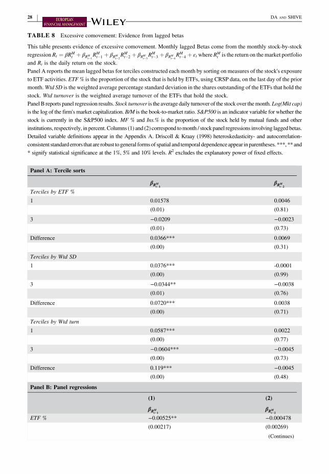
TABLE 8 Excessive comovement: Evidence from lagged betas

This table presents evidence of excessive comovement. Monthly lagged Betas come from the monthly stock-by-stockregressionRt ¼ βRM

t þ βRMt�1RMt�1 þ βRM

t�2RMt�2 þ βRM

t�3RMt�3 þ βRM

t�4RMt�4 þ εt where RM

t is the return on the market portfolioand Rt is the daily return on the stock.Panel A reports the mean lagged betas for terciles constructed each month by sorting on measures of the stock's exposureto ETF activities. ETF % is the proportion of the stock that is held by ETFs, using CRSP data, on the last day of the priormonth.Wtd SD is the weighted average percentage standard deviation in the shares outstanding of the ETFs that hold thestock. Wtd turnover is the weighted average turnover of the ETFs that hold the stock.Panel B reports panel regression results. Stock turnover is the average daily turnover of the stock over themonth.Log(Mkt cap)is the log of the firm's market capitalization. B/M is the book-to-market ratio. S&P500 is an indicator variable for whether thestock is currently in the S&P500 index. MF % and Ins.% is the proportion of the stock held by mutual funds and otherinstitutions, respectively, in percent. Columns (1) and (2) correspond tomonth / stock panel regressions involving lagged betas.Detailed variable definitions appear in the Appendix A. Driscoll & Kraay (1998) heteroskedasticity- and autocorrelation-consistent standarderrors that are robust to general formsof spatial and temporal dependence appear inparentheses. ***, **and* signify statistical significance at the 1%, 5% and 10% levels. R2 excludes the explanatory power of fixed effects.

Panel A: Tercile sorts

βRMt�1

βRMt�2

Terciles by ETF %

1 0.01578 0.0046

(0.01) (0.81)

3 −0.0209 −0.0023(0.01) (0.73)

Difference 0.0366*** 0.0069

(0.00) (0.31)

Terciles by Wtd SD

1 0.0376*** -0.0001

(0.00) (0.99)

3 −0.0344** −0.0038(0.01) (0.76)

Difference 0.0720*** 0.0038

(0.00) (0.71)

Terciles by Wtd turn

1 0.0587*** 0.0022

(0.00) (0.77)

3 −0.0604*** −0.0045(0.00) (0.73)

Difference 0.119*** −0.0045(0.00) (0.48)

Panel B: Panel regressions

(1) (2)

βRMt�1

βRMt�2

ETF % −0.00525** −0.000478(0.00217) (0.00269)

(Continues)

28 | DA AND SHIVE

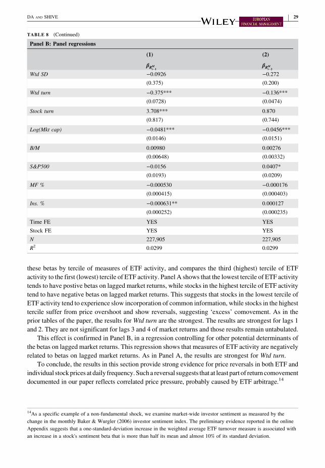
these betas by tercile of measures of ETF activity, and compares the third (highest) tercile of ETFactivity to the first (lowest) tercile of ETF activity. Panel A shows that the lowest tercile of ETF activitytends to have postive betas on lagged market returns, while stocks in the highest tercile of ETF activitytend to have negative betas on lagged market returns. This suggests that stocks in the lowest tercile ofETF activity tend to experience slow incorporation of common information, while stocks in the highesttercile suffer from price overshoot and show reversals, suggesting ‘excess’ comovement. As in theprior tables of the paper, the results for Wtd turn are the strongest. The results are strongest for lags 1and 2. They are not significant for lags 3 and 4 of market returns and those results remain untabulated.

This effect is confirmed in Panel B, in a regression controlling for other potential determinants ofthe betas on lagged market returns. This regression shows that measures of ETF activity are negativelyrelated to betas on lagged market returns. As in Panel A, the results are strongest for Wtd turn.

To conclude, the results in this section provide strong evidence for price reversals in both ETF andindividual stockprices at daily frequency. Such a reversal suggests that at least part of return comovementdocumented in our paper reflects correlated price pressure, probably caused by ETF arbitrage.14

TABLE 8 (Continued)

Panel B: Panel regressions

(1) (2)

βRMt�1

βRMt�2

Wtd SD −0.0926 −0.272(0.375) (0.200)

Wtd turn −0.375*** −0.136***(0.0728) (0.0474)

Stock turn 3.708*** 0.870

(0.817) (0.744)

Log(Mkt cap) −0.0481*** −0.0456***(0.0146) (0.0151)

B/M 0.00980 0.00276

(0.00648) (0.00332)

S&P500 −0.0156 0.0407*

(0.0193) (0.0209)

MF % −0.000530 −0.000176(0.000415) (0.000403)

Ins. % −0.000631** 0.000127

(0.000252) (0.000235)

Time FE YES YES

Stock FE YES YES

N 227,905 227,905

R2 0.0299 0.0299

14As a specific example of a non-fundamental shock, we examine market-wide investor sentiment as measured by thechange in the monthly Baker & Wurgler (2006) investor sentiment index. The preliminary evidence reported in the onlineAppendix suggests that a one-standard-deviation increase in the weighted average ETF turnover measure is associated withan increase in a stock's sentiment beta that is more than half its mean and almost 10% of its standard deviation.

DA AND SHIVE | 29

5 | CONCLUSION

We provide empirical evidence that the arbitrage activity between an exchange-traded fund (ETF) andits underlying portfolio could propagate non-fundamental shocks from the ETFs to a broad cross-section of stocks they hold. In other words, ETF arbitrage could be a new source of return comovement.

We first perform an ETF-level analysis and find that an ETF's turnover is an important determinantof the comovement of the stocks in its portfolio. This result holds controlling for time trend, variousfixed effects and a host of fund-level control variables. In addition, themore an ETF owns of themarketcapitalization of its underlying portfolio, the more the stocks in that portfolio tend to move together.This relationship, however, becomes insignificant after controlling for fund and time fixed effects and ahost of control variables. Finally, the standard deviation of the ETF's daily shares outstanding,capturing creation and redemption activity, is less strongly related to comovement. The link betweenETF activities and return comovement is confirmed in additional tests that exploit the discontinuity inindex membership between two S&P stock indices.

We then perform a stock-level analysis. As in the fund-level analysis, we also find that the weightedaverage turnover of the ETFs that own the stock is related to how much the stock comoves with themarket.We find little evidence that weighted average creation and redemption activity of the ETFs thathold the stock is related to the stock's comovement with the market.

Finally, we find evidence suggesting that some ETF-driven return comovement could be excessive,as reflected by subsequent price reversals at both the fund level and the stock level. At the fund level,we find that the ETF's daily returns are negatively autocorrelated and such an autocorrelation is morenegative when the ETF turnover is higher. These findings support the notion that ETF prices may attimes contain non-fundamental shocks such as price pressure that triggers ETF arbitrage. At the stock-level, we find that stocks with higher measures of ETF activity tend to have significantly negative betason lagged market returns, and that a stock's lagged betas on market returns are negatively related to theactivity of ETFs owning the stock. This suggests that ETF activity is related to overshooting andreversals in prices, a symptom of ‘excess” comovement. In contrast, if ETFs only speed upincorporation of common information, the lagged betas should not be negative.

There is no doubt that the ETF structure provides great benefits. Among others, ETFs provide acheaper and more efficient way for investors to diversify into a broad asset portfolio. At the same time,the results in our paper suggest that they may also lead to ‘excessive’ comovement among these assets.Such ‘excessive’ price comovement could impose costs to institutional investors who trade often andthe costs could even be passed on to many passive individual investors who invest through theinstitutional investors.

REFERENCES

Anton, M., & Polk, C. (2014). Connected stocks. Journal of Finance, 69, 1099–1127.Baker, M., & Wurgler, J. (2006). Investor sentiment and the cross-section of stock returns. Journal of Finance, 61,

1645–1680.Barberis, N., & Shleifer, A. (2003). Style investing. Journal of Financial Economics, 68, 161–199.Barberis, N., Shleifer, A., & Wurgler, J. (2005). Comovement. Journal of Financial Economics, 75, 283–317.Bartram, S. M., Griffin, J. M., Lim, T.-H., & Ng, D. T. (2015). How important are foreign ownership linkages for

international stock returns? Review of Financial Studies, 28, 3036–3072.Ben-David, I., Franzoni, F. A., & Moussawi, R. (2017). Do ETFs increase volatility? Charles A. Dice Center Working

Paper No. 2011-20; Fisher College of Business Working Paper No. 2011-03-20; Swiss Finance Institute ResearchPaper No. 11-66; AFA 2013 San Diego Meetings Paper. Available online at: SSRN: https://ssrn.com/abstract=1967599 or https://doi.org/10.2139/ssrn.1967599

30 | DA AND SHIVE

Boehmer, B., & Boehmer, E. (2003). Trading your neighbor's ETFs: Competition or fragmentation? Journal of Bankingand Finance, 27, 1667–1703.

Driscoll, J., & Kraay, A. (1998). Consistent covariance matrix estimation with spatially dependent data. Review ofEconomics and Statistics, 80, 549–560.

Engle, R., & Sarkar, D. (2002). Pricing exchange traded funds. NYUWorking paper no. S-DRP-02-11, NewYorkUniversity.Forbes, K., & Rigobon, R. (2002). No contagion, only interdependence: Measuring stock market comovements. The

Journal of Finance, 57, 2223–2261.Goetzmann, W., & Massa, M. (2003). Index funds and stock market growth. Journal of Business, 76, 1–28.Greenwood, R. (2008). Excess comovement of stock returns: Evidence from cross-sectional variation in Nikkei 225

weights. Review of Financial Studies, 21, 1153–1186.Greenwood, R., & Sosner, N. (2007). Trading patterns and excess comovement of stock returns. Financial Analysts

Journal, 63, 69–81.Greenwood, R., & Thesmar, D. (2011). Stock price fragility. Journal of Financial Economics, 102, 471–490.Hamm, S. J. W. (2011). The effect of ETFs on stock liquidity. Working paper. Available online at: https://ssrn.com/

abstract=1687914 or https://doi.org/10.2139/ssrn.1687914Harris, L., & Gurel, E. (1986). Price and volume effects associated with changes in the S&P 500: New evidence for the

existence of price pressures. Journal of Finance, 41, 815–829.Hong, H., Kubik, J., & Fishman, T. (2012). Do arbitrageurs amplify economic shocks? Journal of Financial Economics,

103, 454–470.Jiang, W., & Yan, H. (2012). Financial innovation, investor behavior, and arbitrage: Implications from levered

ETFs. Working paper. Available online at: https://ssrn.com/abstract=2023142 or https://doi.org/10.2139/ssrn.2023142.

Kaul, A., Mehrotra, V., & Morck, R. (2002). Demand curves for stocks do slope down: New evidence from an indexweights adjustment. Journal of Finance, 55, 893–912.

Lou, D., & Polk, C. (2013). Comomentum: Inferring arbitrage activity from return correlations. Paul Wooley CentreWorking Paper No. 36, Financial Markets Group Discussion Paper No 721.

Lynch, A., &Mendenhall, R. (1997) New evidence on stock price effects associated with changes in the S&P 500 index,Journal of Business, 70, 351–383.

Marshall, B., Nguyen, N., & Visaltanachoti, N. (2012). The microstructure of arbitrage: ETF evidence.Working paper.Peng, L., & Xiong, W. (2006). Investor attention, overconfidence and category learning. Journal of Financial

Economics, 80, 563–602.Petajisto, A. (2017). Inefficiencies in the pricing of exchange-traded funds. Financial Analysts’ Journal, First Quarter,

24–54.Pollet, J., & Wilson, M. (2008). How does size affect mutual fund behavior? Journal of Finance. 63, 2941–2969.Shleifer, A. (1986). Do demand curves for stocks slope down? Journal of Finance, 41, 579–590.Shleifer, A., & Vishny, R. (1997). The limits of arbitrage. Journal of Finance, 52, 35–55.Staer, A. (2012). Equivalent volume and comovement.Working paper. Available online at: https://papers.ssrn.com/sol3/

papers.cfm?abstract_id=2158462.Wurgler, J. (2010). Challenges to business in the twenty-first century: the way forward. chap. On the Economic

Consequences of Index-Linked Investing (American Academy of Arts and Sciences).Wurgler, J., & Zhuravskaya, E. (2002). Does arbitrage flatten demand curves for stocks? Journal of Business, 75,

583–608.

SUPPORTING INFORMATION

Additional Supporting Information may be found online in the supporting information tab for thisarticle.Table A1: Stock “super-portfolio” betaTable A2: Stock-level tests excluding ETFs holdings less than 100 stocksTable A3: Stock sentiment beta

DA AND SHIVE | 31

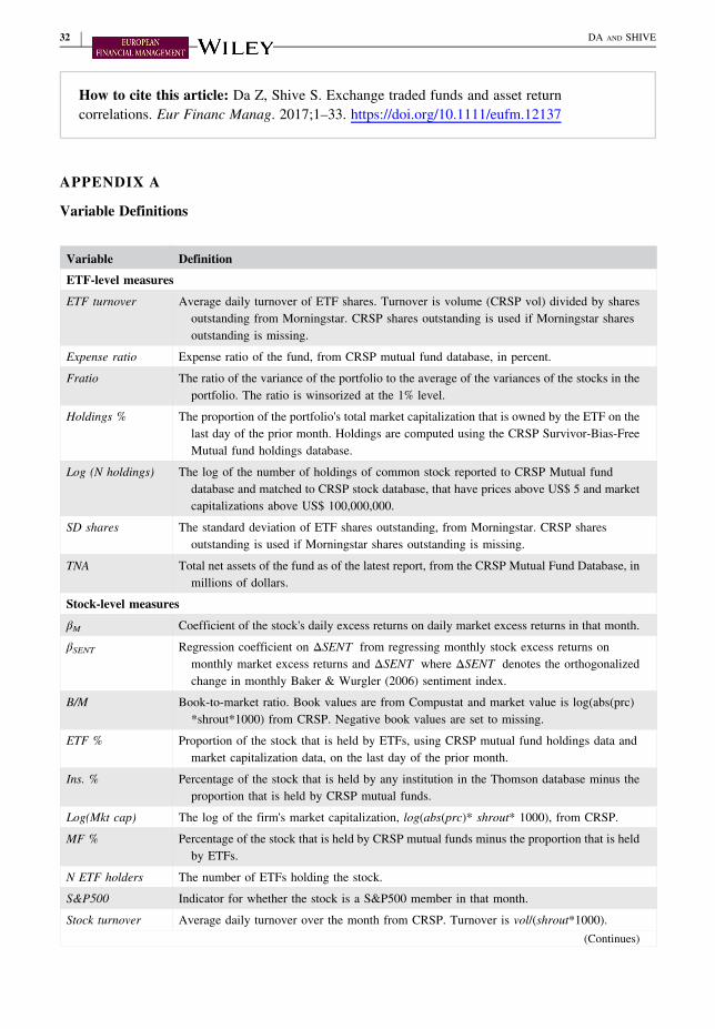
How to cite this article: Da Z, Shive S. Exchange traded funds and asset returncorrelations. Eur Financ Manag. 2017;1–33. https://doi.org/10.1111/eufm.12137

APPENDIX A

Variable Definitions

Variable Definition

ETF-level measures

ETF turnover Average daily turnover of ETF shares. Turnover is volume (CRSP vol) divided by sharesoutstanding from Morningstar. CRSP shares outstanding is used if Morningstar sharesoutstanding is missing.

Expense ratio Expense ratio of the fund, from CRSP mutual fund database, in percent.

Fratio The ratio of the variance of the portfolio to the average of the variances of the stocks in theportfolio. The ratio is winsorized at the 1% level.

Holdings % The proportion of the portfolio's total market capitalization that is owned by the ETF on thelast day of the prior month. Holdings are computed using the CRSP Survivor-Bias-FreeMutual fund holdings database.

Log (N holdings) The log of the number of holdings of common stock reported to CRSP Mutual funddatabase and matched to CRSP stock database, that have prices above US$ 5 and marketcapitalizations above US$ 100,000,000.

SD shares The standard deviation of ETF shares outstanding, from Morningstar. CRSP sharesoutstanding is used if Morningstar shares outstanding is missing.

TNA Total net assets of the fund as of the latest report, from the CRSP Mutual Fund Database, inmillions of dollars.

Stock-level measures

βM Coefficient of the stock's daily excess returns on daily market excess returns in that month.

βSENT Regression coefficient on ΔSENT ⊥ from regressing monthly stock excess returns onmonthly market excess returns and ΔSENT ⊥ where ΔSENT ⊥ denotes the orthogonalizedchange in monthly Baker & Wurgler (2006) sentiment index.

B/M Book-to-market ratio. Book values are from Compustat and market value is log(abs(prc)*shrout*1000) from CRSP. Negative book values are set to missing.

ETF % Proportion of the stock that is held by ETFs, using CRSP mutual fund holdings data andmarket capitalization data, on the last day of the prior month.

Ins. % Percentage of the stock that is held by any institution in the Thomson database minus theproportion that is held by CRSP mutual funds.

Log(Mkt cap) The log of the firm's market capitalization, log(abs(prc)* shrout* 1000), from CRSP.

MF % Percentage of the stock that is held by CRSP mutual funds minus the proportion that is heldby ETFs.

N ETF holders The number of ETFs holding the stock.

S&P500 Indicator for whether the stock is a S&P500 member in that month.

Stock turnover Average daily turnover over the month from CRSP. Turnover is vol/(shrout*1000).(Continues)

32 | DA AND SHIVE

APPENDIX B

Lagged BetaAssume the log stock market index at the end of day t contains a price pressure component, εt,generated by correlated trading in an ETF arbitrage as a large portfolio of stocks are bought and soldsimultaneously. The price pressure on different stocks tends to be in the same direction and thus willnot cancel out at the market level. εt is assumed to follow an AR(1) process:

εt ¼ ρεt�1 þ ηt; 0 < ρ < 1:

A small ρ indices a transitory price pressure. The observed log market daily excess return (ignoringdividends) is:

~rM;t ¼ rM;t þ Δεt;

where rM;t denotes daily market excess return due to fundamental information. The observed logindividual stock excess return can be modelled as:

~ri;t ¼ 1� ϕið ÞβirM;t þ ϕiβirM;t�1 þ λiΔεt þ ξt;

where 1> ϕi > 0 captures slow incorporation of market-wide information and λi > 0 captures theimpact of the market-wide price pressure on stock i. We expect λi to be higher for stocks with moreexposure to ETF activities.

The lagged beta with 1-day lag can be computed as the slope coefficient from regressing ~ri;t on~rM;t�1, or

βRM ;i;1∝Cov ~ri;t;~rM;t� �¼ ϕiβiVar rMð Þ þ λi ρ� 1ð ÞVar εð Þ:

The first term comes from slow incorporation of market information and is positive. The secondterm comes from correlated price pressure and is negative. This is because the transitory price pressuregenerates reversals in daily returns on both the market and the individual stock. A negative lagged betatherefore confirms the presence of correlated price pressure.

(Continued)

Variable Definition

Wtd SD Weighted average percentage standard deviation in the shares outstanding of the ETFs thathold the stock. The weights are proportional to the holdings of each ETF that holds thestock.

Wtd turnover Weighted average turnover of the ETFs that hold the stock. The weights are proportional tothe holdings of each ETF that holds the stock.

DA AND SHIVE | 33