discussion Papers

Discussion Paper 2007-32 July 17, 2007

Measuring Long-Run Exchange Rate Pass-Through

Olivier de Bandt Banque de France, Paris, France

Anindya Banerjee

European University Institute, Firenze, Italy

Tomasz Kozluk European University Institute, Firenze, Italy

Please cite the corresponding journal article: http://www.economics-ejournal.org/economics/journalarticles/2008-6

Abstract: The paper discusses the issue of estimating short- and long-run exchange rate pass-through to import prices in euro area countries and reviews some problems with the measures recently proposed in the literature. Theoretical considerations suggest a long-run Engle and Granger cointegrating relationship (between import unit values, the exchange rate and foreign prices), which is typically ignored in existing empirical studies. We use time series and up-to-date panel data techniques to test for cointegration with the possibility of structural breaks and show how the long-run may be restored in the estimation. The main finding is that allowing for possible breaks around the formation of EMU and the appreciation of the euro starting in 2001 helps restore a long run cointegration relationship, where over the sample period the fixed component of the pass-through decreased while the variable component tended to increase.

JEL: F14, F31, F36, F42, C23 Keywords: exchange rates, pass-through, import prices, panel cointegration, structural break

Correspondence: e-mail: anindya.banerjee@eui.eu, Department of Economics, European University Institute, via della Piazzuola, 43, 50133 Firenze, Italy. Tel.: +39-055-4685-956/927 Fax:+39-055-4685-902. Department of Economics, European University Institute, Firenze, Italy.

The second-named author wishes to thank the Foundation of the Banque de France for their hospitality during his visit in August and September 2005 to the Banque as Visiting Scholar when the first version of this paper was written. He also thanks the Research Council of the EUI for their support. This paper represents the authors' personal opinions and does not reflect the views of the Banque de France or its staff. Comments by Isabelle Méjean and José González Mínguez are gratefully acknowledged.

www.economics-ejournal.org/economics/discussionpapers

© Author(s) 2007. This work is licensed under a Creative Commons License - Attribution-NonCommercial 2.0 Germany

Abstract

The paper discusses the issue of estimating short- and long-run exchange rate pass-through to import prices in euro area countries and reviews some problems with the mea-sures recently proposed in the literature. Theoretical considerations suggest a long-runEngle and Granger cointegrating relationship (between import unit values, the exchangerate and foreign prices), which is typically ignored in existing empirical studies. We usetime series and up-to-date panel data techniques to test for cointegration with the possi-bility of structural breaks and show how the long-run may be restored in the estimation.The main finding is that allowing for possible breaks around the formation of EMU and theappreciation of the euro starting in 2001 helps restore a long run cointegration relationship,where over the sample period the fixed component of the pass-through decreased while thevariable component tended to increase.

Keywords : exchange rates, pass-through, import prices, panel cointegration,structural breaks

JEL classification: F14, F31, F36, F42, C23

Resume

L’article etudie la question de la repercussion a court et a long terme des variationsdu taux de change sur les prix d’importations dans les pays de la zone euro et passe enrevue les indicateurs proposes dans la literature. La theorie economique suggere l’existenced’une relation de cointegration au sens d’Engle et Granger (entre les valeurs unitaires al’importation, le taux de change et les prix e trangers), ce qui est generalement ignoredans les travaux empiriques. Nous utilisons des methodes tres recentes d’analyse des seriestemporelles et d’econometrie des panels en autorisant la presence d’une rupture et montronsque la relation de long terme se retrouve alors dans les donnees. Le principal resultat est quel’introduction de ruptures autour de l’introduction de l’UEM ou de la phase d’appreciationde l’euro a partir de 2001 permet de retrouver une relation de long terme, dans laquelle, surla periode d’echantillon, la partie fixe des prix d’importations se reduit, alors que la partievariable tend a s’accroıtre.

Mots-cles : taux de change, repercussion des chocs, prix d’importation, cointegration surdonnees de panel, ruptures structurelles

Classification JEL : F14, F31, F36, F42, C23

2

Non-technical summary

In the paper, we discuss the issue of estimating short- and long-run exchange rate pass-through to import prices in the countries of the euro area and review some problems with themeasures recently proposed in the literature. Several economic policy issues hang upon thedetermination of the rate of pass-through from exchange rates to prices, and its evolution,both in various time horizons as well as in different sectors. These include issues relating topricing strategies of foreign exporting firms, the persistence of inflation, the likely successof inflation forecasting and the impact of entering into a monetary union.

We first provide a brief review of the theoretical framework of import price formation,which suggests a long-run Engle and Granger cointegrating relationship (between importunit values, the exchange rate and foreign prices). We also present the definition of short-and long-run ERPT assumed by the empirical literature and assess its adequacy. In par-ticular, we look in more detail at some results reported by Campa and Gonzalez Mınguez(2006) (CG hereafter) and show that due to problems of multi-collinearity the distinctionbetween the short- and long-run is somewhat difficult to make, once the statistical signif-icance of the coefficients is taken into account. We compare the CG measures with ourestimates of the Engle-Granger long run wherever these exist, also allowing for structuralbreaks in the cointegrating vector using methods developed by Gregory and Hansen (1996).We show that there is strong evidence of cointegration once account is taken of breaks inthe deterministic components of the cointegrating regressions (such as the constant) andin the cointegrating vector. Interesting contrasts are notably drawn between the long-runcoefficient under the CG definition and those obtained under the specification of a brokenlong run.

In the final part of the paper, we also take advantage of the panel dimension of our datato conduct the analysis of cointegration using panel methods developed by Banerjee andCarrion-i-Silvestre (2006). This is particularly useful in the short-sample analysis where thetime series dimension T is small. The tests used allow not only for breaks in the individualunits of the panel but also for cross-unit dependence. The results seem to confirm stronglythe existence of cointegration, with easily interpretable break dates.

All in all, we use time series and up-to-date panel data techniques to test for cointegra-tion with the possibility of structural breaks and show how the long-run may be restoredin the estimation. The main finding is that allowing for possible breaks around the in-troduction of EMU or the period of appreciation of the euro in 2001 helps restore a longrun cointegration relationship, where over the sample period the fixed component of thepass-through (i.e. the intercept) decreased while the variable component (the elasticity tothe exchange rate) tended to increase.

Resume non technique

L’article etudie la question de l’estimation du degre de transmisssion a court terme et along terme des variations de taux de change aux prix d’importation dans les pays de la zoneeuro. Il passe en revue quelques problemes souleves par les evaluations fournies recemmentdans la litterature economique. Plusieurs questions de politique economique decoulent eneffet de l’analyse de la transmission du taux de change aux prix et de son evolution, a la foisen ce qui concerne l’horizon ou le secteur concerne. Cela inclut notamment des interroga-tions relatives aux strategies de fixation des prix par les firmes etrangeres a l’exportation, ala persistence de l’inflation, aux performances en matiere de prevision de l’inflation et auxeffets de l’entree en union monetaire.

3

L’article presente tout d’abord le cadre d’analyse theorique de la formation des prixd’importation, qui suggere l’existence d’une relation de cointegration au sens d’Engle-Granger (entre les valeurs unitaires a l’importation, le taux de change et les prix etrangers).On rappelle alors la definition generalement retenue dans la litterature econometrique pourla mesure de la transmission des variations du taux de change a court et long terme et sapertinence est discutee. En particulier, l’article analyse en detail certains des resultats deCampa and Gonzalez Mınguez (2006) (notes CG par la suite) et montre que, en raison deproblemes de multi-colinearite, leur estimation de la transmission, ainsi que leur distinctionentre effet a court terme et a long terme, est quelque peu arbitraire. Les estimations deCG sont compares avec celles qui sont tirees de la relation de long terme au sens de Engle-Granger, lorsque celle-ci existe, en autorisant la presence de ruptures structurelles dans levecteur de cointegration selon des methodes developpees par Gregory and Hansen (1996).Au total, de nombreuses elements empiriques militent en faveur de l’existence d’une relationde cointegration lorsque des ruptures sont introduites dans les composantes deterministesdes regressions (par exemple dans la constante) ou dans le vecteur de cointegration luimeme. Il est illustratif de comparer les differences entre les coefficients a long terme tiresde la de finition de CG et ceux de la specification avec rupture a long terme.

Dans la partie finale, l’article exploite la dimension longitudinale des donnees et met enoeuvre une analyse de la relation de cointegration a partir de methode econometriques surdonnees de panel developpees par Banerjee and Carrion-i-Silvestre (2006). Cette approcheest particulierement utile compte tenu de la faible dimension temporelle de nos donnees,ou T est petit. Les tests autorisent non seulement des ruptures pour les series individuellesdu panel mais prennent aussi en compte la dependance entre les unites individuelles. Lesresultats semblent confirmer de facon tres claire l’existence d’une relation de cointegrationavec des dates de ruptures facilement interpretables.

Au total, l’utilisation de techniques econometriques tres recentes dans le domaine del’analyse des donnees de panel et des series temporelles afin de tester l’existence d’unerelation de cointegration en presence de ruptures structurelles conduit a montrer commentla relation de long terme ressort alors naturellement lors de l’estimation. La principaleconclusion est que l’introduction d’une rupture aux alentours de l’introduction de l’UEMet ou lors de la phase d’appreciation de l’euro a partir de 2001 permet de retrouver unerelation de cointegration, pour laquelle, sur l’ echantillon considere, la partie fixe de latransmission (le terme constant) baisse alors que la partie variable (l’elasticite associee autaux de change) tend plutot a s’accroıtre.

4

1 Introduction

A large number of recent papers (see for example Campa and Gonzalez Mınguez, 2006;Campa, Goldberg and Gonzalez Mınguez, 2005; Frankel, Parsley and Wei, 2005; Marazziet al., 2005) have investigated the issue of exchange rate pass-through (ERPT) of foreignto domestic prices. Studies of ERPT have been conducted both for the United States andfor countries of the euro area, with a particular focus on its evolution over the past twodecades, in response to changes in institutional arrangements (such as the inauguration ofthe euro area) and to monetary and financial shocks (such as Black Wednesday and theERM crisis in 1992).

Several economic policy issues hang upon the determination of the rate of pass-throughfrom exchange rates to prices, and its evolution, both in various time horizons as well asin different sectors. These include issues relating to pricing strategies of foreign exportingfirms, the persistence of inflation, the accuracy of inflation forecasts, the impact of enteringinto a monetary union and the success of protocols such as the Lisbon Strategy which callsfor structural reforms across the European Union. For the countries belonging to the euroarea, the issues listed above are particularly relevant.

A notable lacuna in the literature, we argue, is a clear disjunction between the well-worked-out theoretical arguments surrounding the key determinants of pass-through, andthe inappropriate techniques used to estimate import or export exchange rate pass-throughequations. Thus, while almost all the theories contain a long-run or steady-state relationshipin the levels of a measure of import unit values (in domestic currency), the exchange rate(relating the domestic to the numeraire currency) and a measure of foreign prices (unitvalues in the numeraire currency, typically US dollars), this long run is routinely disregardedin most of the empirical implementations. This may seem surprising for at least two reasons.First, proper determination of the short-run ERPT relies on appropriate assumptions aboutthe long run. Second, as monetary policy tends to be medium-term oriented, policy actionsshould in principle look beyond short-term inflation developments for a better understandingof the underlying forces.

Since it is commonly agreed that the time series considered are integrated, one way ofdefining the long run is in the sense of Engle and Granger (1987), henceforth EG, wherethe long run is given by the so-called cointegrating relationship. The reason for ignoringthis long run, and substituting it by an ad hoc measure, is the failure to find evidence inthe data for cointegration. The difficulty inherent in such a re-definition of the long runis two-fold, first the contradiction between a theoretical prediction of a steady state thatcannot be found in the data, and, second, the ad hoc measure proposed being no more thanan extended version of the estimate of the short-run (and, as we shall see below, stronglydominated by the estimated short-run). It is possible that the source of the difficultyis the estimation method used - typically single-equation autoregressive distributed lag(ARDL) models - which may not be powerful enough to verify the theory for the spanof data available. Therefore, instead of looking for a new definition of the long run, amore satisfactory approach is to look for the long-run relationship using more appropriateand powerful methods, such as those which allow for changes in the long run or use morepowerful panel data methods. This is the route we follow in this paper.

Focusing on a specification of ERPT into import prices from Campa, Goldberg andGonzalez Mınguez (2005), we argue in particular that: (a) the long run, in the sense ofEngle and Granger (1987), is restorable once appropriate testing strategies (including laglength selection) are adopted and proper account is taken of the possibility of breaks in

5

the long-run relationship; (b) the estimate of the ‘long run’ used in the empirical literatureis sensitive to a number of misspecification issues; (c) once the distinction is establishedbetween the long run (with a break) in the sense of Engle and Granger (1987) and thedefinition used in the ERPT literature, it becomes important to investigate the relativemagnitudes of these alternative measures and to interpret each differently; and (d) it isimportant to allow for breaks in the long-run theoretical relationship to take due accountof pass-through rates in response to changes in financial regime (such as those followingBlack Wednesday in 1992 or the ERM arrangements which came into force post 1996.) Notto take explicit account of such changes, which are easily evident in the data, could be tomake mistakes in estimation and inference.

We begin in the next section with a very brief overview of the theoretical framework.We next move to the key empirical issues, since these are the main areas of our concern,and in Section 3 establish the key ERPT equation in levels and differences. We presentthe definitions of short- and long-run ERPT assumed by the empirical literature and assesstheir adequacy. Section 4 presents the data.

Section 5 proceeds by looking in more detail at some results reported by Campa andGonzalez Mınguez (2006), CG hereafter. We compare the CG measures with our estimatesof the Engle-Granger long run wherever these exist, also allowing for structural breaksin the cointegrating vector using methods developed by Gregory and Hansen (1996). Weshow that there is strong evidence of cointegration once account is taken of breaks in thedeterministic components of the cointegrating regressions (such as the constant) and in thecointegrating vector.

In Section 6 the analysis of the long run is conducted using panel methods developed byBanerjee and Carrion-i-Silvestre (2006), which are appropriate for looking at cointegrationin panels. This is particularly useful in the short-sample analysis where the time seriesdimension T is small. The tests used allow not only for breaks in the individual units of thepanel but also for cross-unit dependence. The results seem to confirm strongly the existenceof cointegration, with easily interpretable break dates.

Concluding remarks are contained in Section 7 where we discuss whether we shouldreconsider the traditional way of computing the long-run pass-through.1

2 Exchange Rate Pass-Through into Import Prices

By definition,2 import prices for any type of goods j, MP jt are a transformation of export

prices of a country’s trading partners XP jt using the bilateral exchange rate ERt and

dropping superscript j for clarity:

MPt = ERt ·XPt. (1)

In logarithms (depicted in lower case):

mpt = ert + xpt, (2)1Detailed results for single-equation estimates with and without breaks, using the Gregory and Hansen

(1996) algorithm, together with all tables and graphs reproduced for the CG sample 1989-2001 and detaileddescriptions of all tests used are available from the authors upon request.

2This section is based on Campa, Goldberg and Gonzalez Mınguez (2005), CGM hereafter.

6

where the export price consists of the exporters marginal cost and a markup:

XPt = FMCt · FMKUPt. (3)

So that in logarithms we have:

xpt = fmct + fmkupt. (4)

Substituting for xpt into equation (2) yields:

mpt = ert + fmkupt + fmct. (5)

The literature on industrial organization yields insight into why the effect of a change inert on mpt may differ from one, through markup determinants like competitive conditionsthat exporters have to face in the destination markets. Hence, the estimated pass-throughelasticities are a sum of three effects:

• effects of the unity translation effects of the exchange rate movement;

• the response of the markup in order to offset this translation effect;

• the effect on the marginal cost that is attributable to exchange rate movements, suchas the sensitivity of input prices to exchange rates.

Markup responsiveness depends on the market share of domestic producers relative toforeign producers, the form of competition that takes place in the market for the industry,and the extent of price discrimination. Generally, a larger share of imports in total industrysupply, higher degree of price discrimination or a larger share of imported inputs in theproduction in the destination country leads to a higher predicted pass-through. ERPT maybe higher if the ratio of exporters relative to local competitors is high (e. g. for commoditiesor oil), and lower if exporters compete for market shares (e. g. for manufactured goods),even if nominal exchange rate variability is high. Other factors affecting pass-through arethe currency denomination of exports and structure and importance of intermediate goodsmarkets.

The empirical setup of CGM is based on (5) which assumes unity translation of exchangerate movements. However, as mentioned above, exporters of a given product can decide toabsorb some of the exchange rate variations instead of passing them through to the pricein the importing country currency. If the pass-through is complete (producer-currencypricing), their markups will not respond to fluctuations of the exchange rates, thus leadingto a pure currency translation. At the other extreme, they can decide not to vary the pricesin the destination country currency (local-currency pricing or pricing to market) and absorbthe fluctuations within the markup. Thus, markups in an industry are assumed to consist ofa component specific to the type of good, independent of the exchange rate and a reactionto exchange rate movements:

fmkupt = α + Φert. (6)

Also important to consider are the effects working through the marginal cost. These area function of demand conditions in the importing country, marginal costs of production(labor wages) in the exporting country and the commodity prices denominated in foreigncurrency:

fmct = η0 · yt + η1 · fwt + η2 · ert + η3 · fcpt. (7)

7

Substituting (7) and (6) into (5), we have:

mpt = α + (1 + Φ + η2)︸ ︷︷ ︸β

ert + η0 · yt + η1 · fwt + η3 · fcpt + εt, (8)

where the coefficient β on the exchange rate ert is the pass-through elasticity. Obviously,this is a simple approach, with a highly reduced form representation, where one can haveno hope in identifying Φ from η2. In the CGM ‘integrated world market’ specification, theterm η0 ·yt +η1 ·fwt +η3 ·fcpt, independent of the exchange rate, is dubbed the opportunitycost of allocating those same goods to other customers and is reflected in the world priceof the product fpt in the world currency (here taken to be the US dollar).3 Thus the finalequation can be re-written as follows:

mpt = α + β · ert + γ · fpt + εt, (9)

which gives the long run relation between the import price, exchange rate and a measureof foreign price.4

At this point it is perhaps important to stress two issues. First, the exchange rate pass-through literature can be divided in two main streams - with papers which focus on ‘firststep’ pass-through, i.e. ERPT into import prices and those which consider ‘second step’pass-through, i.e. into consumer prices. As has been made clear above, for the purpose ofthis paper we will look only at ERPT into import prices.

The second issue concerns the fact that since ERPT is a channel linking exchange rateswith prices, it is often named as one of the key determinants of monetary policy design.There is a vast literature on optimal monetary policy, starting with models developed for aclosed economy, and extended to the open economy (see for example Obstfeld, 2002).

Importantly, much of the focus of the Stochastic Dynamic General Equilibrium literatureconcentrates on short-run pass-through, and assumes that pass-through in the long-run isfull (see, among others, Smets and Wouters, 2002; Adolfson, 2001). This is usually the resultof the existence of staggered price setting, which allows the response to an exchange rateshock with imperfect adjustment in the short run, because of menu costs, and a gradual fullincorporation of the change in the long run. On the other hand the literature focusing onprice discrimination allows imperfect pass-through in the long run, as part of the adjustmentis borne by firms’ markup (this issue is reviewed in more detail in Corsetti, Dedola andLeduc, 2005). In the latter paper, the introduction of an intermediary sector which uses non-

3The integrated market hypothesis in CG is based on the assumption that there exists a single worldmarket for each good. Therefore, regardless of the origin of the product, on the world market, it has oneworld price. This price constitutes the opportunity cost of selling to a local market. Thus, in the CGsetup for the integrated market and, consequently, in ours, it proxies for the foreign price. The currencydenomination does not in fact matter, as long as the exchange rate for the local currency is taken vis-a-visthis ’world’ currency. In the CG case the extra-euro area imports denominated in US dollars are takenas a proxy for the world price. This might be seen as a strong assumption, but, by taking data from anhomogeneous database of IUVs for both import prices and world price, this avoids introducing additionalmeasurement errors in the analysis.

4It is not uncommon in the literature to insert additional control variables on the right hand side ofthis equation. For example, Marazzi et al. (2005) use commodity prices, in order to control for changes inmarginal costs that producers may face. This seems undesirable in our specifications for at least two reasons.First, we are concerned with ERPT in individual sectors, and thus the appropriate equation for commoditysectors will already contain the commodity price - thus the control variable would be redundant. Second,and more generally any marginal cost effect is assumed to work through the ’world price’.

8

traded intermediate goods creates a long-run wedge between world prices in local currencyand domestic prices.

As we will show, there is some evidence that ERPT into import prices, is not always fulleven in the long run. These results points to the invalidity of the full-ERPT assumption andmay have important implications for the proper estimation of the short-run pass-throughand consequently the design of monetary policy. Importantly, this finding seems more inline with the price discrimination models as in Corsetti, Dedola and Leduc (2005).

Admittedly, there is a large degree of endogeneity in the observed ERPT and monetarypolicy. That is, pricing strategies of firms depend not solely on competition conditions inthe market, but also on monetary policy, or rather the expected future monetary policyand the policy makers’ credibility. The formation of the Economic and Monetary Union,which occurs in the middle of the sample period used for the empirical exercise, is thuslikely to have an important impact on ERPT (while the ERPT level itself may affect thestrength, and exact timing of the break) and any estimation method should take accountof these changes. This is our guiding motivation for looking at long run relationships withstructural change in our study of ERPT.

3 ERPT - estimation

Both economic theory and relevant tests lead us to think each of the series (import price,exchange rate and world price) as being characterized by a unit root. However, despitethe underlying levels equation (1), CG are not able to reject the null hypothesis of thenon-existence of a cointegrating relationship among the three series. Hence, they proceedby estimating equation (9) in first differences:

∆mpt = a +4∑

k=0

bk ·∆ert−k +4∑

k=0

ck ·∆fpt−k + εt, (10)

for a certain type of good i in a certain country j. The superscripts have been omittedfor clarity. Next, they define the coefficient b0 and the sum of coefficients

∑4k=0 bk as the

short-run and long-run ERPT respectively.At this point it is useful to focus on the CG definition of the long-run pass-through.

Since CG do not find evidence of the long run in the Engle and Granger (1987) sense, incommon with much of the literature in this area, they use the definition of the long rungiven by equation 10 above. We argue that the CG definition of the long-run pass-through,which is constructed by summing the estimated coefficients for the first five lags (i.e. lag0 to lag 4), is somewhat difficult to justify, and thus rather inadequate for the purpose ofenquiring about the actual long-run effect. For example, it is not clear why five lags arechosen. This measure further does not take into account the significance of the coefficientson the individual lags, for which there is a great deal of evidence of multi-collinearity.Taking for example the estimates for France (see Table 1) we can see that in the majorityof cases only the coefficient on lag 0 is significant, while the following four lags are notsignificantly different from 0. As these coefficients are of relatively large magnitude, thenumber of lags is rather important - if one summed the first three, four, or six lags, thepoint estimate of the long run could differ vastly, though potentially would be as justified.The joint significance of the sum of the coefficient-estimates is generally not to be doubted,but the high uncertainty surrounding the individual estimates does lead to difficulties in

9

France

Lag 0 Lag 1 Lag 2 Lag 3 Lag 4 CG LRSITC0 0.96 -0.03 -0.01 -0.15 -0.04 0.74

(0.09) (0.11) (0.11) (0.11) (0.08) (0.10)SITC1 0.01 0.59 -0.49 0.71 -0.41 0.40

(0.2) (0.25) (0.26) (0.25) (0.21) (0.25)SITC2 0.77 0.16 0.05 0.06 -0.06 0.98

(0.11) (0.13) (0.13) (0.13) (0.1) (0.13)SITC3 1.06 -0.02 0.1 -0.05 0.07 1.16

(0.06) (0.07) (0.08) (0.08) (0.06) (0.08)SITC4 1.13 -0.14 -0.31 0.36 -0.08 0.97

(0.25) (0.3) (0.31) (0.31) (0.24) (0.33)SITC5 0.87 0.08 -0.11 -0.12 0.1 0.81

(0.17) (0.19) (0.19) (0.19) (0.15) (0.26)SITC6 1.11 -0.26 0.22 0.09 -0.17 1.00

(0.09) (0.11) (0.11) (0.11) (0.08) (0.09)SITC7 1.12 -0.3 0.25 -0.02 -0.01 1.03

(0.14) (0.15) (0.15) (0.15) (0.12) (0.22)SITC8 0.95 -0.17 0.11 -0.11 -0.01 0.76

(0.08) (0.1) (0.11) (0.1) (0.07) (0.12)

For each sector first line reports the estimated coefficient,and the second the standard error.

Table 1: Estimates of equation (10) - coefficients and standard errors on the lags of exchangerate - original CG sample 1989-2001. The last column reports the CG long-run estimate.

interpretation. The importance of our argument for inference can be illustrated further bytaking the coefficients for SITC0 from Table 1 - the CG long run is significantly differentfrom 1, while if we redefine the ‘long run’ as the sum of the first three lags, we could notbe able to reject it being equal to 1. With SITC1 the example becomes even more visible- the five-lag CG long run is insignificantly different from 0, while significantly differentfrom 1, whereas the four-lag ‘long run’ would be significantly different from 0, while notdiffering significantly from 1. Similar patterns of fluctuation of the coefficient estimates arealso observed for some other sectors in Table 1 (and for other countries). We also repeatthe analysis by re-estimating the equation with four lags or six lags and reach similarconclusions. Details are available from us upon request.

The fact that CG are unable to find a cointegrated ‘equilibrium’ relationship between thevariables in levels may seem surprising in light of the fact that the theoretical underpinningof the ERPT, is in fact a levels relationship, as in equation (1). We proceed by notingthat if the cointegrated equilibrium relationship were to exist, the equation to be estimatedshould contain an error correction term (ECM), as in Engle and Granger (1987), and thustake the following form:

∆mpt = a+K1∑

k=0

bk ·∆ert−k+K2∑

k=0

ck ·∆fpt−k+λ(mpt−1 − α− β · ert−1 − γ · fpt−1︸ ︷︷ ︸ECM

)+ut, (11)

while equation (10) would be misspecified.

10

There are a number of reasons which could lead to a failure to find a cointegrating rela-tionship in series which are suspected to be cointegrated. In particular, as we show below,appropriate lag length selection and proper accounting for a structural break, whether insingle equations or more powerful panel methods, can change the inference on the existenceof a ‘long-run’ relationship. This helps to provide a less arbitrary estimate of the long-runERPT and to assess changes to this elasticity following the introduction of the euro. Wediscuss these issues in Section 5, following a brief description of the data in Section 4 below.

4 Data

In order to perform our estimations, we use two data sets. The original sample, approx-imately equivalent to the one used by CG contains data for import unit values (in localcurrency), exchange rates (relative to US dollar) and world prices (denominated in USdollars) for 1-digit SITC sectors for 11 countries. As noted in the previous section, weconcentrate on looking at the integrated market specification, although analogous resultsmay be derived under ‘segmented’ markets, where the index of world price (or unit values)is constructed as a weighted (by trade shares) geometric average of prices of each country’sfive largest trading partners.

The CG data set covers the years 1989-2001 and serves mainly to illustrate that thechange of methodology would also result in changes in the inference of the original CGpaper. Results of the estimations for this sample are available from the authors. Moreimportant for our specific goals we use the sample of 1995-2005, from Eurostat, whichhas the advantage of extending further beyond the suspected break date related to theintroduction of the euro than the previous data set. The construction of the variablesfollows CG, and is described in the Appendix A.

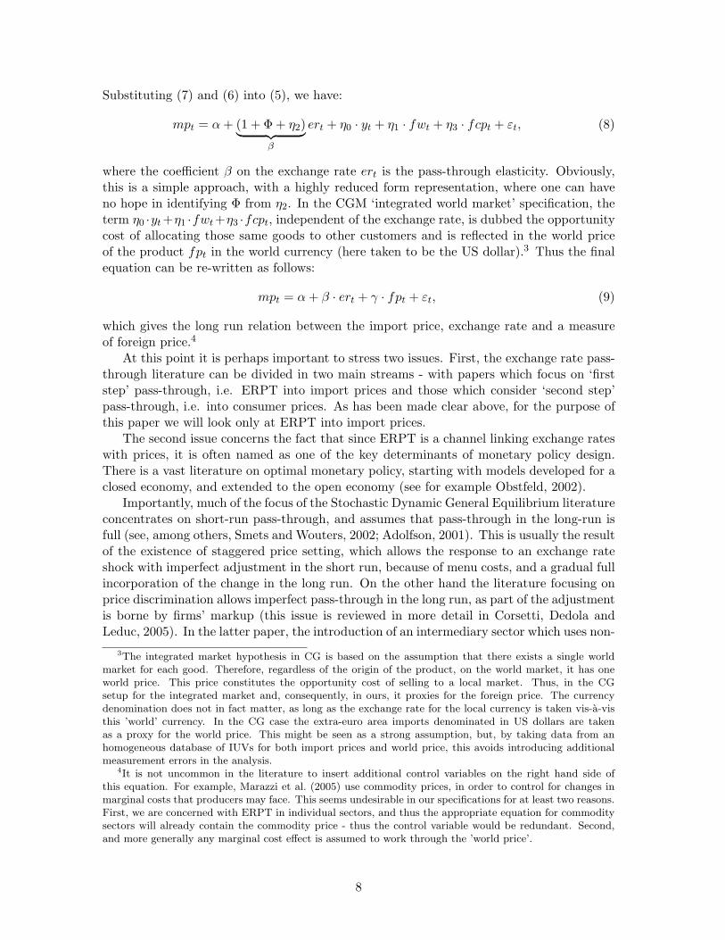
Figure 1: Monthly index of exchange rates of euro area currencies versus the USD. 1995-2005.

The indicator we use for import prices, the index of import unit values (IUV) has aseries of caveats concerning their use that must be kept in mind. First of all, unit values,as provided by Eurostat are values of kilograms of a certain good. This means we are

11

looking for instance not only at kilograms of food, oil or raw materials, but also kilogramsof computers, cars etc. Moreover, following CGM, we consider the 1-digit SITC industries asa reasonable compromise between the informative power of the series and their availabilityand frequency. Using IUVs, means the ‘goods’ we speak of are not well defined goods as such- they are in fact bundles of goods (of all goods that are traded on the certain month and fallinto the specific SITC category) and thus the composition of such bundles may change frommonth to month (apart from being different from country to country). Additionally, thiscomposition may change precisely because of changes in the exchange rate, as the demand(and supply) and thus the pricing strategy of some specific sub-category goods may be verydifferent especially within categories as wide as SITC 8 Misc. Manufactured goods. Thusthe part of the adjustment to the exchange rate change that will go through quantity andnot price, will affect the implicit weight of the good in our 1-digit SITC basket.

These cautions having been stated, it remains the case that we are constrained in ourinvestigations by the quality of the publicly available data. While there may be numerousdoubts about using IUVs as a proxy for import prices, the lack of alternative measures(especially at a sectoral level) forces us to use what is available. This has the advantagethat we can make comparisons with the CG or CGM estimates which are based on similarlyconstructed data.

Further, following from our discussion in Section 2, it is important to emphasize thatthere are a number of reasons why we expect there may be a change in the long-run ERPTwithin our sample.

Firstly, on the 1st of January 1999, 11 European countries fixed their exchange rates byadopting the euro.5 This constituted a change in monetary policy, especially for countrieswere such policy was previously less credible. The perceived stabilization of monetarypolicy, especially in countries with previously rather less successful monetary policy, mayhave induced the producers to change their pricing strategies, and thus have an influence onthe ERPT. We expect the formation of the euro area to have caused a change in long-runERPT, though this change may have commenced both before the exact adoption date, forinstance upon joining the ERM, as well as after, when the euro became a well establishedcurrency.

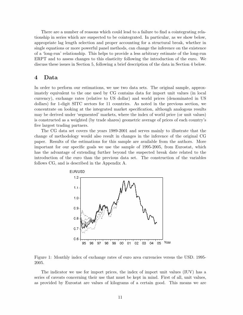
Figure 2: Residuals from the estimation of equation (9) without a break (left) and with asingle estimated break (right) on the series for Spain, SITC0.

5Greece failed to fulfil the Maastricht Treaty criteria, and therefore joined 2 years later, effective 1st ofJanuary 2001.

12

Anticipating to some extent our future results, on left hand side of Figure 2 we show theerrors from the estimation of the levels equation (9), for which as we will see in Section 5.1it is quite hard to reject the null hypothesis of non-stationarity. On the right hand, we havethe residuals from the same equation once we allow for a break - these seem to appear morestationary. The substantial changes in the behavior of the residuals commence, as may benoted in the figure, in the run-up to the euro. Similar figures may be constructed e.g. forFrance which again shows significant change around the end of 1998. This goes somewhatahead of our argument, to which we will return to it in more detail in Section 5.2, but servesfor the purpose of illustrating that not accounting for a structural break in the relationshipmay lead us to the failure of finding a long run, although we must be constantly vigilantthat what we classify as a ‘break’ is not a data artifact. We have good reasons for believingthis not to be the case.

Moreover the adoption of a common currency has changed the competitive conditions,by increasing the share of goods denominated in the (new) domestic currency, hence trulycreating a single market for exporters.

Finally, looking at the exchange rates of current euro area currencies in Figure 1 we seethat in virtually all the countries the currencies were depreciating against the US dollar inthe period 1995-2000, and especially since 1996. Moreover, after a short period of a stableeuro dollar exchange rate, the euro currency(ies) started appreciating, till the end of oursample. This asymmetry of exchange rate developments may have different implicationsfor the ERPT, as obviously for an imported good with a fixed dollar price, depreciation ofthe euro vis-a-vis the dollar would mean the increase of the price of the good on the euroarea market, while the appreciation of the euro, a decrease of the price, leading to possiblydifferent behavior of the producers’ margin.

5 Results

5.1 Single equations - without breaks (importance of lag length selection)

Simple augmented Dickey-Fuller tests for cointegration in single time series for individualcountry/industry combinations (see Table 2) do not support the CG view about the lack ofcointegration between the series. The results concern the more recent sample (1995-2005)yet by switching to automatic lag selection criteria we manage to obtain rejections of thenull of no cointegration for a vast majority of the series (at 5% level). Moreover, adoptinginformation criteria chosen lag length when testing the null on the 1989-2001 CG sample,leads to the rejection of the null of no cointegration for most of the series.6 Therefore wecan say that there is some evidence that a long-run relationship in levels, in the sense ofEngle and Granger (1987), exists among our variables.

5.2 Single equations, with structural breaks

In order to pursue the issue of looking for cointegrating relationships further, we propose theuse of the Gregory and Hansen (1996, GH hereafter) algorithm which allows for testing thenull of no cointegration against the alternative of cointegration with an estimated structuralbreak. We test two alternative versions of the model proposed in equation (9). First, a break

6Details on the exact same exercise done for the CG 1989-2001 sample are available from the authors.

13

H0:

Uni

tro

ot(n

oco

inte

grat

ion)

Cou

ntry

SIT

C0

SIT

C1

SIT

C2

SIT

C3

SIT

C4

SIT

C5

SIT

C6

SIT

C7

SIT

C8

Fran

ce-2

.75∗∗∗

-2.6

9∗∗∗

-3.0

6∗∗∗

-3.1

1∗∗∗

-1.8

5∗-5

.51∗∗∗

-5.4

7∗∗∗

-3.6

5∗∗∗

-4.1

2∗∗∗

Net

herl

ands

-2.5

1∗∗

-3.1

5∗∗∗

-3.3∗∗∗

-2.9

7∗∗∗

-2.6

1∗∗∗

-3.1

4∗∗∗

-2.1∗∗

-3.4

2∗∗∗

-6.4

7∗∗∗

Ger

man

y-1

.51

-2.2

9∗∗

-2.4

6∗∗

-4.9

4∗∗∗

-3.7

7∗∗∗

-3.7

9∗∗∗

-2.2

1∗∗

-6.6

5∗∗∗

-5.7∗∗∗

Ital

y-1

.93∗

-1.6

9∗-2

.45∗∗

-2.7

2∗∗∗

-4.1

1∗∗∗

-3.4

1∗∗∗

-2.3∗∗

-2.8∗∗∗

-1.9

2∗

Irel

and

0.2

-2.1

3∗∗

-4.9

8∗∗∗

-5.2

6∗∗∗

-2.2

1∗∗

-9.3

1∗∗∗

-2.9

8∗∗∗

-5.0

6∗∗∗

-4.2

1∗∗∗

Gre

ece

-1.8

2∗-1

.93∗

-2.2

8∗∗

-2.7

3∗∗∗

-2.0

6∗∗

-4.2

9∗∗∗

-2.9

1∗∗∗

-3.4

7∗∗∗

-3.0

8∗∗∗

Por

tuga

l-2

.48∗∗

-1.8

2∗-2

.9∗∗∗

-4.3

1∗∗∗

-1.5

9-9

.13∗∗∗

-2.1

6∗∗

-4.2

4∗∗∗

-2.6

6∗∗∗

Spai

n-1

.95∗∗

-2.2

7∗∗

-3.6

5∗∗∗

-3.8∗∗∗

-2.3∗∗

-4.0

2∗∗∗

-2.1

5∗∗

-3.6

2∗∗∗

-5.5

5∗∗∗

Fin

land

-0.7

6-7

.76∗∗∗

-2.2∗∗

-2.6

2∗∗∗

-3∗∗∗

-3.9

1∗∗∗

-3.4

7∗∗∗

-2.7

5∗∗∗

-6.3

6∗∗∗

Aus

tria

-6.4

9∗∗∗

-2.2

6∗∗

-3.5

3∗∗∗

-4.6

5∗∗∗

-2.4

3∗∗

-8.1

4∗∗∗

-2.9∗∗∗

-2.6

3∗∗∗

-6.4

4∗∗∗

AD

Ft-st

atis

tic,

***,

**,*

-th

enu

llhy

poth

esis

isre

ject

edat

99%

,95

%an

d90

%re

spec

tive

ly.

Spec

ifica

tion

:no

cons

tant

,no

tren

d.M

axim

umla

gsnu

mbe

r=

12.

Lag

select

ion:

Aka

ike

(AIC

).

Tab

le2:

AD

Fte

stson

the

erro

rsfr

omth

eO

LS

regr

essi

onof

the

‘long

-run

’equ

atio

n(9

).Sa

mpl

e:19

95-2

005.

Tes

tre

sult

sw

ith

alte

rnat

ive

lag-

sele

ctio

ncr

iter

iaar

eav

aila

ble

from

the

auth

ors.

14

in the constant, thus a level shift:

mpt = α + α1 ∗ ds + β · ert + γ · fpt + εt, (12)

thus we allow for a slope shift (i.e. a change in the elasticity of the long-run pass-through)in addition to a shift in the level:

mpt = α + α1 ∗ ds + β · ert + β1 · ert ∗ ds + γ · fpt + γ1 · fpt ∗ ds + υt. (13)

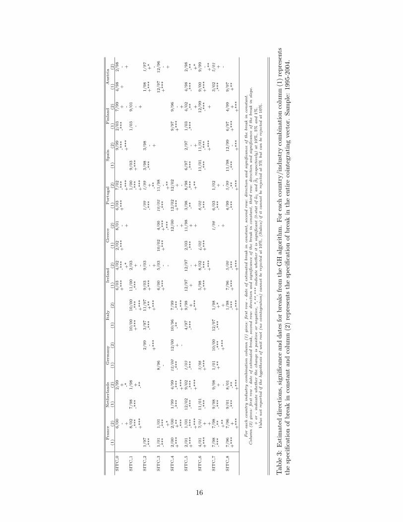
In both cases ds is a dummy variable equal to 0 if t < s and equal to 1 otherwise. The GHalgorithm allows for the estimation of the break point s positioning it where the ADF test onerrors from the estimated levels equation yield the strongest evidence for the rejection of thenull hypothesis of no cointegration.7 It is an issue of considerable interest to decide whichformulation of the model to adopt. We provide evidence below to show that it is the secondof the two formulations that we would tend to choose. Generally, as mentioned earlier,upon the introduction of the euro, we would expect the fixed component of the markup(denoted by the coefficient α) to fall rather than increase - due to potentially improvedcompetition in the market arising from increased price transparency. Table 3 (for the GHsingle-equation tests8) shows clearly that in the specification that allows for only a breakin the constant, the fixed component in the markup tends to rise roughly in as many casesas it tends to fall. However as the specification from equation (12) is much more restrictivethan the one based on equation (13), not allowing for a possible break in the other variableswould tend to cause the estimate of α1 to be biased. Table 3 shows that the more flexiblespecification of a break in slope and constant lead to the majority of the estimates pointingto a decrease or insignificant change in the fixed markup component. In more detail, whenwe allow for the more general break as in equation (13), for the GH single equations for40 out of 61 series α1’s are negative (of which 24 are significant at 10%), leaving only 7positive and significant (at 10%).

Comparing the results for the two alternative specifications (with breaks in constantand with breaks in constant and slope) we see that in a handful of cases the rejection of thenull of no cointegration was possible when the alternative did not allow for a break, whilenot possible when the alternative accounted for a break. This tends to suggest, that inthese cases the evidence for the existence of a break is weak.9 Overall the most important

7Brief details of the procedure are contained in Appendix B.8In order to save space, we report only the directions, significance and dates of breaks estimated with the

GH algorithm. These are reported in Table 3 if the null hypothesis of unit root (i.e. no cointegration) canbe rejected at 10%. As for the coefficient estimates, they are essentially very similar to the ones in Table 5for the break in constant specification and Table 6 for the break in entire cointegrating vector specification,as the Banerjee and Carrion-i-Silvestre (2006) adaptation of the Pedroni (1999) test to account for breaksbuilds on the GH specification. However, due to data availability the single-equation GH estimation is basedon a longer (by one year 1995) series for all countries except Finland and Austria.

9If for a certain series we are able to reject the null of no cointegration against an alternative of coin-tegration without a break (ADF), but unable to do so against an alternative with a break (GH), this maybe evidence that there is no break in the cointegrating relationship. The reasoning is as follows. We treatrejection of the null of no cointegration (ADF) as evidence of existence of a cointegrating relationship be-tween the variables, as in equation (9). In this case, imposing a break, i.e. a dummy variable as in equation(12), or a dummy variable with interaction variables as in equation (13), would mean adding variables of noexplanatory power (insignificant) and should not in principle affect our statistic. However, the critical valuesof the GH tests are higher in absolute value than those of the standard ADF test, in order to guaranteeappropriate test sizes for the null of no cointegration against of an alternative of cointegration with a break.Thus a more or less unaffected test statistic and a higher critical value may result in the failure to reject the

15

Fra

nce

Neth

erl

ands

Germ

any

Italy

Irela

nd

Gre

ece

Port

ugal

Spain

Fin

land

Aust

ria

(1)

(2)

(1)

(2)

(1)

(2)

(1)

(2)

(1)

(2)

(1)

(2)

(1)

(2)

(1)

(2)

(1)

(2)

(1)

(2)

SIT

C0

6/00

2/99

6/03

4/02

2/02

8/01

6/03

7/02

9/99

2/03

7/99

4/98

2/98

-+

+***

-***

+***

-+

***

-***

-***

-***

++

-+

-*+

*+

+***

+***

-+

SIT

C1

8/02

7/98

1/98

10/00

10/00

11/00

2/03

1/00

9/03

1/03

9/01

-***

-***

++

***

-***

-***

+-*

**

+***

--

+***

-**

+***

-+

***

+SIT

C2

1/97

2/99

3/97

11/97

9/03

9/03

1/99

1/99

3/98

3/98

1/98

1/97

-***

--*

**

+**

+***

--*

**

+-*

**

-+

***

+*

+***

+***

+-*

*+

-SIT

C3

1/01

1/01

8/96

6/00

5/03

10/02

4/00

10/02

11/98

12/97

12/96

-***

-***

-+

***

-+

***

+***

-***

-+

***

-+

*-

-***

+**

+SIT

C4

2/00

2/00

1/99

4/99

12/00

12/00

10/96

7/99

12/00

12/02

12/02

9/97

9/96

+***

+**

-***

-***

-***

+-*

*-*

**

-+

***

++

***

--*

**

+***

-+

***

+-

+SIT

C5

2/01

1/01

12/02

9/02

1/03

4/97

9/98

12/97

12/97

2/03

11/98

3/98

8/98

6/97

2/97

1/03

4/02

4/98

2/98

+***

-***

-***

-***

-***

-***

++

--*

**

+-*

*-*

**

-***

--*

**

-**

-***

-**

+***

+***

+***

++

+**

++

+*

SIT

C6

4/01

7/01

11/01

3/98

5/98

8/02

4/02

8/02

11/01

11/01

12/99

9/00

9/99

+***

+-*

**

+***

+***

-***

+***

-***

-***

-***

-***

+***

-+

+***

+***

++

**

SIT

C7

7/98

7/98

9/98

9/98

1/01

10/00

12/97

1/98

1/98

6/03

1/02

3/02

5/01

-***

-**

-***

++

**

-***

-***

+*

--*

**

+-*

**

++

**

-+

***

++

--

SIT

C8

7/96

7/96

9/01

8/01

1/98

7/96

5/00

4/99

5/99

11/98

12/99

6/97

4/99

9/97

+***

+-*

**

-**

-***

+***

-***

-***

-**

-***

-+

***

++

**

+***

+***

+***

+***

+***

+***

+***

For

each

countr

yin

dust

ry

com

bin

ation

colu

mn

(1)

giv

es:

first

row

-date

ofest

imate

dbre

ak

inco

nst

ant,

seco

nd

row:

direc

tion

and

signifi

cance

ofth

ebre

ak

inco

nst

ant.

Colu

mn

(2)

giv

es:

first

row

-date

ofest

imate

dbre

ak,se

cond

row:

direc

tion

and

signifi

cance

ofth

ebre

ak

inco

nst

ant,

third

row:

direc

tion

and

signifi

cance

ofth

ebre

ak

inslope.

+or

-in

dic

ate

wheth

er

the

change

isposi

tive

or

neg

ative,*,*

*,*

**

indic

ate

wheth

er

itis

signifi

cant(t

-sta

tof

α1

and

β1

resp

ectively

)at10%

,5%

and

1%

.Valu

enotre

porte

dif

the

hypoth

esi

sofunit

root(n

oco

inte

gra

tion)

cannotbe

reje

cte

dat10%

,(I

talics)

ifit

cannotbe

reje

cte

dat5%

butca

nbe

reje

cte

dat10%

.

Tab

le3:

Est

imat

eddi

rect

ions

,sig

nific

ance

and

date

sfo

rbr

eaks

from

the

GH

algo

rith

m.

Forea

chco

untr

y/in

dust

ryco

mbi

nati

onco

lum

n(1

)re

pres

ents

the

spec

ifica

tion

ofbr

eak

inco

nsta

ntan

dco

lum

n(2

)re

pres

ents

the

spec

ifica

tion

ofbr

eak

inth

een

tire

coin

tegr

atin

gve

ctor

.Sa

mpl

e:19

95-2

004.

16

outcome is that in a relatively short sample, there are only about 12 out of 90 series forwhich we are unable to reject the null of no cointegration in any of the three specifications(no break, break in constant, breaks in slopes). We treat this as strong evidence of thepresence of a theory-backed long-run relationship in the data, which changes in response tokey economic events.10

A selection of the single-equation results for the ‘long-run’ ERPT are presented in Fig-ures 3 and 4. As indicated in the notes to the figures, they present the point estimateand the 95% confidence interval for both the CG-defined long run (estimator (1) in all thefigures) i.e. the sum of five lags, as well as the EG long run in 5 different specifications.Noticeably, apart from yielding different values of the pass-through, the EG estimates aremore precise which allows for more definite conclusions regarding the rejection or acceptanceof the hypotheses of ERPT being equal to 0 or 1. The narrower confidence intervals arean immediate consequence of the superconsistency of the OLS estimator in a cointegratingrelationship. The coefficients obtained from the estimation of equation (9) when allowingfor a structural break in the entire cointegration vector (observations (4) and (5) for theGH estimated break and (7), (8) for the imposed 1998/1999 break) may, however, be moreimprecise, especially if the estimated break happens to lie towards the beginning or end ofthe sample.

There is some country- and industry-specific variety in long-run pass-through, wherecommodity sectors (SITC 2 and SITC 3) tend to have a higher (closer to 1) pass-throughthan manufacturing sectors, and with very few exceptions we can strongly reject zero ratesof pass-through. A glance at the tables and figures also suggests, if anything, an increase inthe pass-through rates in most countries and most industries, with some exceptions. Notall of these changes are significant, but the tendency is nevertheless rather clear cut.

Overall, tests for cointegration, be it without a break, with a break in the constant,or in the entire ”equilibrium” relationship allow us to reject the null of no cointegrationtherefore providing support for the existence of a long run relationship as in equation (9) inour data. This stands somewhat in contrast with the CG conclusion that no cointegratingrelationship exists, and allows us to switch from an arbitrary definition of long-run ERPTas a sum of five (mostly insignificant) coefficients on the lags of the exchange rate to thelong run in the EG sense.

The evidence gathered above, by looking at individual sectors within each country canbe strengthened even further by using several recently developed panel-based tests for coin-tegration. Dealing with single time series, albeit with about 110-120 observations, we stillhave a time span of only about 10 years of data. However, by looking at the evidence fromall the sectors and countries together (if the number of sectors in each country, is 9 andthere are 10 countries in our data set, a panel-based test could use up to 9 × 10 × 110observations) and allowing for heterogeneity, we should in principle obtain a far clearer ideaof the common trends underlying the series and hence the existence of the long run. Inthe spirit of the discussion above, any such estimation procedure in panels would of courseneed to allow for structural change. In addition it would also need to allow for dependenceamong the units of the panel. We turn now to a consideration of these issues.

null in the case when imposing a break is not justified.10The changes are modelled here as discrete breaks in constant or slope and is a limitation of our framework.

A richer alternative to consider would be allow for non-linearities, which may in fact pick up evidence forgradual change. This is unfortunately precluded in our study by the shortage of data.

17

Figure 3: France - ‘long-run’ ERPT estimates with confidence intervals (95%). Individualindustries, sample: 1995-2005, entire sample analysis. The estimators are presented in thefollowing order: (1) CG long run, no cointegration, no break, (2) cointegrating long-run,no break, (3) cointegrating long run, break in constant (estimated, GH), (4) cointegratinglong run before break in slope (estimated, GH), (5) cointegrating long run, after break(estimated, GH), (6) cointegrating long run, break in constant (imposed on 1998/99), (7)cointegrating long run, before break in slope (imposed on 1998/99), (8) cointegrating longrun, after break (imposed on 1998/99). In (3)-(5) values extracted from GH algorithm,ADF*. Values not reported if no cointegration (ADF). Break dates estimated with theGH are available together with equivalent graphs for Germany and Portugal in De Bandt,Banerjee and Kozluk (2006). Dotted horizontal line at value of 1.

18

Figure 4: Italy - ‘long-run’ ERPT estimates with confidence intervals. Individual industries,sample: 1995-2005. Notes - see Figure (3) for explanations.

19

6 Panel cointegration tests

There are essentially three ways of proceeding in order to construct panels from the data sets- (1) creating country panels of industry cross-sections, (2) industry panels with countrycross-sections and (3) a pooled panel in which every country and industry combinationconstitutes a separate unit. In search of the existence of a cointegrating relationship in theseries we try to maximize the dimensions of our panel, and thus will focus on (3). Hencewe will apply two types of tests. The so called first generation panel cointegration tests asin Pedroni (1999) test for existence of a cointegrating relationship, assuming no cross-unitinterdependence. The modification of the test, based on Gregory and Hansen (1996) isproposed in Banerjee and Carrion-i-Silvestre (2006) and allows for an estimated breakpointin each individual series. As mentioned however, the tests have the shortcoming of notaccounting for possible cross unit dependence. This, as shown by Banerjee, Marcellino andOsbat (2004) in a series of Monte Carlo simulations, can lead to substantial oversize of thetests, and thus increase the possibility of wrongful rejection of the null of no cointegration.

The second generation of tests, as the one proposed in Banerjee and Carrion-i-Silvestre(2006) allows a factor structure for cross-section dependence, while allowing for an individ-ual, estimated break date.11 The statistics for the Pedroni (1999) panel cointegration tests

Model pseudo-t pseudo-ρNo break -7.73 -35.45Break in constant (eq. 12) -22.15 -49.38Break in constant andslope (eq. 13)

-23.26 -49.50

Under the null hypothesis both statistics havea N(0,1) distribution

Table 4: Parametric statistics fot the panel cointegration test. The null hypothesis is nocointegration. Sample: 1996-2004, full panel (N=90), unit specific breaks, no cross-sectiondependance. See Appendix B for details.

with no cross-sectional dependence and no breaks are displayed in the first row of Table 4.They allow for strong rejection of the hypothesis of no cointegration even when the alter-native does not allow for a break. This test is restrictive in the sense that we do not allowthe cointegration relationship to change within our sample. However as mentioned, we sus-pect the formation of the euro area constituted a shift in both competition conditions andmonetary policy which may have affected the long-run pass-through. We propose runningthe Pedroni (1999) test which allows for the change in the cointegrating vector. The resultsallow strong rejection of the null of no cointegration in both the case of a shift in constantand break in the cointegrating relationship between the variables for all the country panels.By construction the test chooses the break date which is consistent with strongest evidenceagainst the null. The test algorithm allows us to extract the break dates for each individualseries, as well as the cointegrating coefficients. These are presented in Tables 5 and 6.

Within the context of these results derived from the panel tests, it is useful to returnbriefly to the issue of model choice and to ask whether the more flexible formulation (i.e.equation (13) instead of (12)) is also the more appropriate here. We note from the panel es-

11Brief details of these tests are contained in Appendix B.

20

timates reported in Table 6 that out of 90 series, 60 have a negative estimated α1 coefficient,of which in 35 cases they are significant, while only for 10 they are significantly positive.We therefore point to the break in slope and constant specification as being more coherentwith the idea that the fixed component of the markup falls (a negative value of α1), whilechanges in the pass-through are also observed for a number of sectors and countries.12 The

Figure 5: Distribution of estimated break dates in half-year intervals (1997s1-2003s2).Breaks in slope taken from Tables 6. Dark color - all breaks, light color - only breakswhen long-run ERPT changed significantly (10%).

estimated break dates for all the individual series are presented in Figure 5. There is somedispersion among the obtained dates, though there seem to be two modes of the distribution- one relatively close to the introduction of the euro and the other close to the turn-aroundin the euro/dollar exchange rate developments (2000-2001).

Although the evidence, as presented in Tables 5 and 6, in favor of both cointegrationand structural change is unequivocally strong, a few qualifications are worth noting. First,the GH based algorithm here allows for only one, ”strongest” break,13 which is a seriouslimitation as far as timing the (single) break allowed is concerned. Second, as noted earlierwhen referring to non-linear methods, the effect of the change in macroeconomic conditionson the ERPT may not have been either instantaneous or linear. Finally, there are otherfeatures of this period which are relevant, such as the evolution of the euro/pound rate forIreland, late euro area membership for Greece etc.

Nevertheless, the sheer fact that despite these limitations (which would in all cases haveacted against us) the algorithm identifies a relatively large amount of series where there iscointegration and change, be it upon the introduction of the euro, or upon the appreciationof the euro, is an interesting finding. Moreover, as we will turn to the interpretation of

12It is worth noting that also in the case of the specification with the break in constant only, 52 out of 90of the estimated changes in the constant are negative (51 of which significant at 10%) though admittedlymany more are significantly positive (38) than in the case of the more flexible specification (break in constantand slope) which we treat as an argument in favor for the latter. This is in line with the argument thatthe formation of the EMU may have increased the power of ’domestic currency denominated’ products, orreduced uncertainty associated with the exchange rate leading to a fall in the constant markup componentcharged by ’foreign currency denominated’ products.

13In fact it does not touch upon the notion of the strength of evidence of the break. Generally the breakfound by this algorithm is a break for which the evidence for a cointegrating relationship is the strongest(i.e. largest - in absolute value - test statistic leading to the rejection of the null of no cointegration).

21

‘Lon

g-ru

n’ex

chan

gera

tepa

ss-t

hrou

ghco

effici

ents

Indu

stry

Fran

ceN

ethe

rlan

dsG

erm

any

Ital

y(1

)(2

)(3

)(1

)(2

)(3

)(1

)(2

)(3

)(1

)(2

)(3

)SI

TC

00.

880.

912

/97

0.63

0.63

8/03

0.89

0.85

3/02

0.98

0.76

9/98

(0.0

3)(0

.03)

–***

(0.0

3)(0

.03)

–***

(0.0

6)(0

.03)

–***

(0.0

8)(0

.05)

–***

SIT

C1

0.72

0.77

9/03

0.34

0.7

5/98

0.81

0.57

3/98

0.54

0.23

10/0

0(0

.06)

(0.0

7)–*

(0.0

6)(0

.08)

–***

(0.0

3)(0

.04)

+**

*(0

.07)

(0.0

8)+

***

SIT

C2

0.98

1.06

5/97

0.76

0.81

2/98

0.78

0.85

12/9

70.

981.

15/

97(0

.03)

(0.0

3)–*

**(0

.03)

(0.0

3)–*

**(0

.02)

(0.0

2)–*

**(0

.03)

(0.0

3)–*

**SI

TC

30.

960.

973/

010.

850.

777/

981.

11.

049/

001.

081.

156/

00(0

.02)

(0.0

1)–*

**(0

.04)

(0.0

4)+

***

(0.0

2)(0

.02)

+**

*(0

.02)

(0.0

2)–*

**SI

TC

40.

210.

822/

001.

361.

3312

/98

1.21

1.1

10/0

10.

20.

256/

97(0

.14)

(0.1

1)+

***

(0.0

5)(0

.05)

–***

(0.0

6)(0

.06)

–***

(0.1

3)(0

.13)

–*SI

TC

50.

520.

689/

990.

50.

5710

/02

0.51

0.55

2/98

0.45

0.66

4/98

(0.0

3)(0

.06)

–***

(0.0

3)(0

.04)

–***

(0.0

2)(0

.03)

–*(0

.04)

(0.0

5)–*

**SI

TC

60.

860.

827/

010.

851.

031/

010.

850.

763/

980.

991.

2710

/99

(0.0

1)(0

.01)

+**

*(0

.03)

(0.0

2)–*

**(0

.02)

(0.0

1)+

***

(0.0

3)(0

.03)

–***

SIT

C7

0.46

0.54

4/98

0.62

0.89

10/9

80.

550.

484/

000.

30.

441/

98(0

.02)

(0.0

2)–*

**(0

.03)

(0.0

4)–*

**(0

.01)

(0.0

3)+

**(0

.02)

(0.0

2)–*

**SI

TC

80.

740.

76/

980.

680.

869/

010.

740.

783/

030.

540.

831/

98(0

.01)

(0.0

2)+

***

(0.0

3)(0

.04)

–***

(0.0

1)(0

.02)

–***

(0.0

4)(0

.02)

–***

For

each

coun

try

and

indu

stry

com

bina

tion

colu

mns

:(1

)fir

stro

w:

coeffi

cien

twhe

nno

brea

kal

lowed

,se

cond

row:

stan

dard

erro

r;(2

)fir

stro

w:

coeffi

cien

tif

shiftin

cons

tant

allo

wed

,se

cond

row:

stan

dard

erro

r;(3

)fir

stro

w:

estim

ated

shiftda

tefo

rco

lum

n(2

),se

cond

row:

dire

ctio

nan

dsi

gnifi

canc

eof

shiftin

cons

tant

;*,

**,*

**de

note

shiftin

cons

tant

issi

gnifi

cant

(t-s

tatof

α1)

at10

%,5%

and

1%re

spec

tive

ly.

+an

d–

deno

tepo

sitive

and

nega

tive

shifts

inco

nsta

nt

Tab

le5:

Pan

elco

inte

grat

ion

(Ped

roni

1999

,m

odifi

edin

Ban

erje

ean

dC

arri

on-i-S

ilves

tre,

2006

,to

acco

unt

for

brea

ks)

resu

lts

wit

hout

brea

ks(e

quat

ion

(9))

and

wit

hbr

eaks

inco

nsta

nt(e

quat

ion

(12)

),re

port

edfo

rgr

oup

pseu

do-t

.C

ross

-sec

tion

:in

divi

dual

indu

stry

inan

indi

vidu

alco

untr

y.N

ocr

oss-

sect

ion

depe

nden

ce.

Sam

ple:

1996

-200

4.

22

‘Lon

g-ru

n’ex

chan

gera

tepa

ss-t

hrou

ghco

effici

ents

Indu

stry

Irel

and

Gre

ece

Por

tuga

lSp

ain

(1)

(2)

(3)

(1)

(2)

(3)

(1)

(2)

(3)

(1)

(2)

(3)

SIT

C0

0.45

0.48

6/03

0.47

0.3

8/01

0.61

0.61

9/03

0.73

0.69

2/00

(0.1

2)(0

.08)

+**

*(0

.06)

(0.0

4)+

***

(0.0

8)(0

.05)

+**

*(0

.05)

(0.0

4)+

***

SIT

C1

-0.5

7-0

.12

11/0

00.

480.

355/

020.

260.

4412

/02

1.1

0.93

9/03

(0.0

9)(0

.11)

–***

(0.0

3)(0

.03)

+**

*(0

.12)

(0.1

4)–*

*(0

.08)

(0.0

8)+

***

SIT

C2

0.68

0.59

9/03

0.54

0.36

7/00

0.4

0.74

5/99

0.83

0.97

3/98

(0.0

5)(0

.05)

+**

*(0

.03)

(0.0

4)+

***

(0.0

5)(0

.05)

–***

(0.0

4)(0

.03)

–***

SIT

C3

0.72

0.86

5/03

0.99

1.23

7/02

1.04

1.1

3/00

1.14

1.18

6/97

(0.0

5)(0

.06)

+**

*(0

.1)

(0.0

7)+

***

(0.0

3)(0

.04)

–**

(0.0

2)(0

.02)

–***

SIT

C4

0.31

0.54

9/01

0.64

0.64

10/0

10.

421.

4112

/02

0.64

0.71

5/99

(0.1

1)(0

.11)

+**

*(0

.14)

(0.1

1)+

***

(0.2

4)(0

.19)

+**

*(0

.09)

(0.0

9)+

***

SIT

C5

0.48

0.51

3/02

0.5

0.54

1/01

0.58

0.72

3/98

0.61

0.76

11/9

7(0

.02)

(0.0

3)–

(0.0

1)(0

.02)

–**

(0.0

5)(0

.07)

–**

(0.0

3)(0

.04)

–***

SIT

C6

0.74

0.61

7/98

0.81

0.69

12/0

10.

570.

738/

020.

730.

856/

02(0

.03)

(0.0

2)+

***

(0.0

3)(0

.03)

+**

*(0

.04)

(0.0

3)–*

**(0

.03)

(0.0

2)–*

**SI

TC

70.

560.

5110

/97

0.51

0.4

11/9

70.

350.

378/

030.

310.

4110

/98

(0.0

3)(0

.04)

+*

(0.0

2)(0

.03)

+**

*(0

.02)

(0.0

2)–*

*(0

.02)

(0.0

2)–*

**SI

TC

80.

610.

459/

990.

920.

752/

020.

530.

76/

980.

650.

9212

/99

(0.0

4)(0

.08)

+**

(0.0

3)(0

.04)

+**

*(0

.04)

(0.0

5)–*

**(0

.03)

(0.0

6)–*

**N

otes

:se

epr

evio

uspa

ge.

Tab

le5:

cont

inue

d.

23

‘Lon

g-ru

n’ex

chan

gera

tepa

ss-t

hrou

ghco

effici

ents

Indu

stry

Fin

land

Aus

tria

(1)

(2)

(3)

(1)

(2)

(3)

SIT

C0

0.86

0.92

5/00

0.68

0.69

4/98

(0.1

)(0

.05)

–***

(0.0

4)(0

.04)

–***

SIT

C1

0.72

0.73

3/03

0.17

0.6

3/99

(0.0

3)(0

.03)

–***

(0.0

7)(0

.08)

–***

SIT

C2

1.14

0.74

4/99

0.76

0.72

1/98

(0.0

7)(0

.06)

+**

*(0

.02)

(0.0

2)+

***

SIT

C3

1.01

0.87

4/99

0.98

0.87

12/9

7(0

.03)

(0.0

4)+

***

(0.0

3)(0

.03)

+**

*SI

TC

40.

250.

119/

970.

040.

6111

/00

(0.1

1)(0

.1)

+**

*(0

.13)

(0.1

2)+

***

SIT

C5

0.49

0.55

11/0

20.

270.

44/

98(0

.03)

(0.0

3)–*

**(0

.03)

(0.0

5)–*

**SI

TC

60.

750.

710

/98

0.56

0.44

9/00

(0.0

2)(0

.02)

+**

*(0

.02)

(0.0

2)+

***

SIT

C7

-0.0

60.

123/

020.

160.

253/

02(0

.03)

(0.0

3)–*

**(0

.02)

(0.0

2)–*

**SI

TC

80.

440.

365/

970.

610.

579/

97(0

.02)

(0.0

3)+

***

(0.0

2)(0

.03)

–***

Not

es:

see

prev

ious

page

.

Tab

le5:

cont

inue

d.

24

‘Lon

g-ru

n’ex

chan

gera

tepa

ss-t

hrou

ghco

effici

ents

Indu

stry

Fran

ceN

ethe

rlan

dsG

erm

any

Ital

y(1

)(2

)(3

)(1

)(2

)(3

)(1

)(2

)(3

)(1

)(2

)(3

)SI

TC

00.

840.

966/

000.

621.

211

/02*

**0.

890.

934/

000.

751.

729/

00**

*(0

.03)

(0.1

2)–

(0.0

3)(0

.18)

–**

(0.0

3)(0

.11)

+(0

.05)

(0.1

5)–*

**SI

TC

10.

541.

94/

02**

*0.

80.

598/

980.

670.

424/

98**

*0.

211.

533/

99**

*(0

.07)

(0.3

6)–*

**(0

.08)

(0.1

2)–

(0.0

5)(0

.07)

+**

(0.1

1)(0

.18)

–***

SIT

C2

1.03

0.85

5/02

0.91

0.77

2/98

**0.

780.

8812

/98*

**0.

891.

175/

00**

*(0

.03)

(0.1

3)+

**(0

.06)

(0.0

3)–

(0.0

3)(0

.02)

–(0

.04)

(0.0

4)–

SIT

C3

0.99

1.13

5/00

***

1.13

0.87

6/00

**1.

051.

12/

991.

071.

146/

00(0

.02)

(0.0

2)–*

**(0

.07)

(0.0

7)+

(0.0

7)(0

.03)

–(0

.04)

(0.0

4)–

SIT

C4

1.13

0.45

2/00

***

1.08

1.3

4/99

**1.

120.

7812

/00*

*-0

.58

0.77

6/99

***

(0.1

6)(0

.13)

+**

(0.0

8)(0

.05)

–***

(0.0

8)(0

.12)

+*

(0.2

2)(0

.13)

–***

SIT

C5

0.52

0.79

9/99

**0.

581.

272/

00**

*0.

440.

787/

00**

00.

7612

/98*

**(0

.08)

(0.0

8)–*

**(0

.08)

(0.1

9)–*

**(0

.04)

(0.1

4)–*

*(0

.12)

(0.0

6)–*

**SI

TC

60.

810.

817/

011.

011.

122/

01**

0.66

0.78

1/01

***

1.09

1.42

12/9

9***

(0.0

2)(0

.04)

–(0

.02)

(0.0

4)–*

(0.0

2)(0

.04)

–***

(0.0

4)(0

.04)

–***

SIT

C7

0.46

0.58

11/9

81.

050.

9412

/98

0.45

1.12

9/00

***

0.35

0.44

1/98

(0.0

8)(0

.02)

–(0

.12)

(0.0

4)+

(0.0

2)(0

.12)

–***

(0.0

7)(0

.02)

+SI

TC

80.

710.

76/

980.

841.

369/

01**

0.8

0.41

3/03

*0.

580.

861/

98**

*(0

.05)

(0.0

2)+

(0.0

6)(0

.2)

–**

(0.0

2)(0

.2)

+**

(0.0

7)(0

.02)

–***

For

each

coun

try

and

indu

stry

com

bina

tion

colu

mns

:(1

)fir

stro

w:

coeffi

cien

ton

ER

befo

rebr

eak,

seco

ndro

w:

stan

dard

erro

r;(2

)fir

stro

w:

coeffi

cien

ton

ER

afte

rbr

eak,

seco

ndro

w:

stan

dard

erro

r;(3

)fir

stro

w:

estim

ated

shiftda

tewith

sign

ifica

nce

ofch

ange

inco

effici

enton

ER

,se

cond

row:

dire

ctio

nan

dsi

gnifi

canc

eof

shiftin

cons

tant

;*,

**,*

**de

note

shiftis

sign

ifica

nt(t

-sta

tof

β1

orα

1)

at10

%,5

%an

d1%

resp

ective

ly.

+an

d–

deno

tepo

sitive

and

nega

tive

shifts

inco

nsta

nt

Tab

le6:

Pan

elco

inte

grat

ion

(Ped

roni

,19

99,m

odifi

edin

Ban

erje

ean

dC

arri

on-i-S

ilves

tre,

2006

,to

acco

unt

for

brea

ks)

resu

lts

from

spec

ifica

tion

asin

equa

tion

(13)

,rep

orte

dfo

rgr

oup

pseu

do-t

.C

ross

-sec

tion

:in

divi

dual

indu

stry

inan

indi

vidu

alco

untr

y.N

ocr

oss-

sect

ion

depe

nden

ce.

Sign

ifica

nce

test

sba

sed

ontr

adit

iona

lt-

stat

s.Sa

mpl

e:19

96-2

004.

25

‘Lon

g-ru

n’ex

chan

gera

tepa

ss-t

hrou

ghco

effici

ents

Indu

stry

Irel

and

Gre

ece

Por

tuga

lSp

ain

(1)

(2)

(3)

(1)

(2)

(3)

(1)

(2)

(3)

(1)

(2)

(3)

SIT

C0

0.42

0.9

5/02

*0.

210.

737/

98**

*0.

581.

914/

02**

*0.

621.

2910

/99*

**(0

.06)

(0.2

7)–*

**(0

.06)

(0.0

9)–*

**(0

.05)

(0.2

8)–*

**(0

.03)

(0.1

1)–*

**SI

TC

1-0

.33

-0.4

22/

030.

310.

125/

020.

361.

411/

030.

790.

877/

02(0

.1)

(0.8

1)–

(0.0

3)(0

.23)

+(0

.14)

(1.0

8)–

(0.1

)(0

.53)

–SI

TC

20.

570.

667/

020.

390.

277/

000.

780.

581/

99*

0.99

0.96

3/98

(0.0

5)(0

.23)

–(0

.05)

(0.0

9)+

(0.0

9)(0

.06)

+(0

.06)

(0.0

3)+

SIT

C3

0.88

0.93

5/03

1.12

-0.2

5/00

***

0.96

1.03

11/9

80.

971.

063/

00*

(0.0

6)(0

.48)

–(0

.11)

(0.1

4)+

***

(0.1

1)(0

.04)

+(0

.03)

(0.0

3)+

SIT

C4

0.82

0.61

1/01

0.67

0.9

7/01

1.54

0.78

12/0

20.

351.

276/

00**

*(0

.14)

(0.1

7)+

(0.1

2)(0

.25)

–(0

.21)

(0.4

7)+

(0.1

3)(0

.15)

–***

SIT

C5

0.27

0.47

12/9

70.

530.

418/

99**

0.28

0.76

8/98

**0.

410.

817/

00*

(0.1

4)(0

.04)

–(0

.04)

(0.0

4)+

**(0

.19)

(0.0

9)–*

**(0

.07)

(0.2

2)–

SIT

C6

0.57

0.9

8/02

***

0.64

0.49

12/0

10.

921.

1711

/99*

**0.

91.

242/

01**

*(0

.03)

(0.1

)–*

**(0

.03)

(0.1

2)+

(0.0

6)(0

.05)

–**

(0.0

2)(0

.04)

–***

SIT

C7

0.55

1.05

11/0

10.

190.

411

/97

0.37

0.38

11/0

20.

40.

389/

98(0

.04)

(0.4

3)–

(0.1

3)(0

.03)

–**

(0.0

2)(0

.31)

+(0

.08)

(0.0

2)–

SIT

C8

0.52

1.16

9/00

**0.

740.

132/

02*

0.34

0.81

8/98

***

1.05

1.08

12/9

9(0

.09)

(0.2

3)–*

**(0

.06)

(0.3

1)+

*(0

.13)

(0.0

6)–*

**(0

.07)

(0.1

)+

Not

es:

see

prev

ious

page

.

Tab

le6:

cont

inue

d.

26

‘Lon

g-ru

n’ex

chan

gera

tepa

ss-t

hrou

ghco

effici

ents

Indu

stry

Fin

land

Aus

tria

(1)

(2)

(3)

(1)

(2)

(3)

SIT

C0

0.86

0.73

10/0

00.

690.

792/

99(0

.04)

(0.1

3)+

*(0

.05)

(0.1

2)–

SIT

C1

0.71

1.01

3/02

0.64

0.5

3/99

(0.0

4)(0

.2)

–(0

.09)

(0.1

9)+

SIT

C2

0.63

0.82

4/99

0.77

0.72

1/98

(0.0

9)(0

.07)

–**

(0.0

6)(0

.03)

+*

SIT

C3

0.72

0.9

4/99

0.75

0.88

12/9

7(0

.1)

(0.0

4)–*

(0.1

)(0

.03)

–SI

TC

4-0

.17

0.12

9/97

0.91

0.07

7/00

***

(0.3

4)(0

.11)

–(0

.17)

(0.1

9)+

***

SIT

C5

0.47

0.81

4/03

0.21

0.46

2/99

*(0

.03)

(0.2

8)–*

*(0

.1)

(0.0

7)–*

*SI

TC

60.

720.

7412

/00

0.43

0.51

9/00

**(0

.02)

(0.0

4)–*

*(0

.02)

(0.0

3)–

SIT

C7

0.2

1.19

11/0

1***

0.27

0.23

5/02

(0.0

3)(0

.32)

–***

(0.0

3)(0

.25)

+SI

TC

80.

590.

494/

000.

580.

5612

/98

(0.0

6)(0

.11)

+(0

.07)

(0.0

3)–

Not

es:

see

prev

ious

page

.

Tab

le6:

cont

inue

d.

27

developments in individual countries and sectors in the following section we will observesome interesting patterns in estimated break points.

We consider the test results from the panel as sufficient evidence in favor of the exis-tence of a ‘long-run’ levels relationship between the variables, as implied by the theoreticalunderpinning - equation (9). Moreover, despite some variability in the estimated breaks inthe individual series we can say that at least for some country/industry combinations thereis evidence that the formation of the EMU led to a significant change in the equilibriumpass-through rate, be it directly upon its formation or indirectly by tying the currency to theeuro, and thus seeing it appreciate against the dollar since about 2001. However, as given

H0: unit root (no co-integration)

No. of fac-tors

Pseudo-t - ADF ce (i)∗

No break Break (a) Break (b) Break (c) Break (d)(1) -4.51 -3.72 -3.11 -4.51 -2.66(3) -3.71 -3.47 -2.60 -3.33 -2.59(6) -3.76 -2.95 -3.47 -4.44 -3.22

Under the null the statistics have the normal N(0, 1) distribution.No break, (a) - common break in constant imposed on 1998/1999,

(b) common break in the entire co-integrating relationship, imposed on 1998/1999,(c) - country-specific, estimated break as in equation (12),(d) - country-specific, estimated break as in equation (13),

∗ - See Appendix B for description.

Table 7: Test statistics for Banerjee and Carrion-i-Silvestre (2006) panel co-integration testswith cross-section dependence (common factors). Sample: 1996-2005.

above, the failure of first generation panel cointegration tests to account for cross sectiondependence tends to oversize the tests and may lead to flawed inference on the existence ofthe long run relationship. Our final generalization of the testing framework, having alreadydeveloped tests for cointegration with structural breaks, is to allow for a factor structureto model this type of dependence (as in Bai and Ng, 2004) and apply the test proposed byBanerjee and Carrion-i-Silvestre (2006) which allows for a unit specific estimated break inthe series. In this second generation test, we test the null of no cointegration against analternative hypothesis of cointegration (with up to r common factors modeling cross sectiondependence) with one common break date for all the series (1998/1999) and for individ-ual estimated break dates for each country. Due to the construction of the test, which isbased on the extraction of common factors from the error terms, the break and coefficientestimates are obtained with exactly the same first-generation tests conducted before andthus there is no need to repeat them. The results for 1-, 3- and 6-factor dependence struc-tures are reported in Table 7 and we consider them as reconfirmation of the existence of along-run equilibrium relationship.

Having discussed the breaks, we can now turn to analyzing the actual long-run pass-through estimates in more detail.

We will focus on the coefficients in Table 6 as the most general setting, which allows forbreaks in both the constant and the cointegrating vector. The increase in ERPT in mostsectors in countries like Italy, Spain and Portugal usually coincides with the introduction ofthe euro. This may be a sign of the increase in the credibility of the monetary regime, that

28

occurred when these countries joined the euro area, which led foreign producers to expectmore stable conditions, and as argued below made them more willing to pass on the actualfluctuations. This change is not evident in the case of Greece, which generally has ratherlow pass-through rates, but joined the euro 2 years later, and experienced in the run-up toEMU a much more significant downward shift in inflation than the other countries. Thismay explain the particular pattern of the latter country.

As for the sectors, notably sector SITC 5 (Chemical products) faced an increase (signif-icant in 7 of the 10 countries) in pass-through across almost all the countries in question,rendering it closer to 1. Next, in SITC 0 (Food and live animals) there has been an increasein the pass-through in the Netherlands, Italy, Ireland, Greece, Portugal and Spain fromvalues around 0.5 to values much closer to 1. The estimated dates of this change are closeto the euro introduction for Italy, Greece and Spain. For the Netherlands, Ireland andPortugal the estimated breaks lie in mid 2002 and even in 2003. In the case of Ireland, anexplanation for this may be provided by her intensive trade ties with the United Kingdom,which is by far the most important origin of imports into that country. As opposed tothe euro/dollar exchange rate, the euro/sterling rate was relatively stable throughout oursample (see Figure 6). Specifically the British pound did not depreciate against the euroas the dollar did since about 2001. Thus euro movements versus the dollar may have hadmuch lesser influence on the pass-through in this country, and suggests the weakness of theintegrated world market assumption for Ireland. Finally in all the specifications it is evidentthat the pass-through in sector SITC3, i.e. mineral fuels, is practically equal to or very closeto 1, and has not changed substantially upon the introduction of the euro. This may beexplained by strong market power of foreign producers in this sector, who face practicallyclose to zero domestic competition in products like oil, and thus a common world price isfully passed on when the exchange rate fluctuates.

7 Discussion and concluding remarks

The results of our paper show ample evidence for an EG cointegrating relationship betweenthe variables in levels - as in the underlying theoretical equation (9). We have suggestedseveral methods for working with the data that enable the cointegrating relationship to bedetected, including better lag-length selection in the tests for cointegration and a consid-eration of the impact of structural change and conducting inference using a panel (wherethe N dimension augments the T ). By taking care of the adverse effects of cross-sectiondependence, we have shown that the evidence from the panel tests - with or without al-lowing for structural breaks - is entirely unambiguous. Thus, even if one were not willingto accept the notion of ‘detectable’ structural change, as modeled in this paper, or wereonly willing to attribute the finding of a break to data issues, it should be noted that ourmain contentions would still hold. We can therefore redefine the long-run effect of exchangerate fluctuations on prices to be consistent with the theoretical literature. Instead of arather arbitrary sum of (mainly insignificant, of opposite signs) coefficients on lags of theexchange rate,14 which we discussed in Section 3, we propose using the EG cointegratingequation coefficient. The use of the standard measure of pass-through should be viewedwith caution, or re-interpreted substantially.

Our main preoccupation is the fact that despite using data of monthly frequency and14This would, as we have argued, make the estimates problematic to interpret in any case - regardless of

whether the notion of a long run, defined as the sum of four or five short-run effects, is coherent.

29

aiding ourselves with panel methods, we still deal with a relatively short sample of at most10 years. This may prove too short for the ‘true’ long run to reveal itself. This problemis aggravated by the specific developments in our sample - namely the introduction of theeuro, the Maastricht criterion de facto restricting the bilateral movements of the exchangerates of the countries since 1997, and the depreciation and subsequent appreciation of theeuro-dollar rate.

However, we think that the sheer fact that we find overwhelming evidence in favor of acointegrating relationship in the EG sense provides backing to the presence of a theoreticallyimplied relationship as in equation (9). Augmenting this finding with our techniques for(a) dealing with change in the sample; and (b) extracting information from a panel, wherepooling or averaging over the 90 units counteracts the noise arising from the T dimension,makes our case more compelling.

When discussing the long-run ERPT, anticipating our discussion of the results below,a number of other issues arise concerning the magnitude of the pass-through coefficient asmeasured by us. First of all, can we reasonably expect to have less than full ERPT inthe long run? Most of the literature, see for example Smets and Wouters (2002), is basedon the notion that nominal rigidities cause imperfect ERPT. ’But since rigidities such assticky prices tend to be a short- to medium-run phenomenon, one may be led to thinkthat producers would be unwilling to accommodate a change in the exchange rate into hismarkup forever, thus leading us to expect full ERPT in the long run.

This story is not entirely convincing - the foreign exporter maximizes profit, not markupover a set of markets and over time, and thus may be willing to accept adjustments to hismarkup in order to maintain market share, adapting to competitive conditions both inthe short and long run. The fact that empirically, exchange rates are found to be muchmore volatile than prices, would also suggest that even in the long run, not all exchangerate fluctuations are passed on to the price level and some of the adjustment may be donethrough quantity. Consequently, Corsetti, Dedola and Leduc (2005) propose a model whereERPT is lower than one even in the long run, as a result of price discrimination and thusdifferent pricing strategies between markets. Thus overall, a finding of the exchange ratepass-through to be lower than one also in the long run is not unreasonable.

Finally, in this context, can we expect the long-run ERPT to be greater than 1? Essen-tially, in the long run, the answer is ‘no’. We do find a handful of the series exhibiting anERPT estimate significantly greater than one. However, most commonly this occurs whenwe allow for a break in the slope and the break is estimated as being located rather closeto the end of the sample, making inference unreliable.

Before proceeding to a discussion of the estimated break dates, their location, and thedirection and nature of the change in the cointegrating relationships, we should emphasizethat both our single-equation and panel methods allow for only a single break. This is alimitation imposed by the relatively short span of our sample. If there are, say, two breaks inthe data, the algorithm may pick up only one of them, or estimate a break lying somewherein between the two actual breaks. This may account for some of the heterogeneity reportedin the tables.

Generally speaking, both in our single-equation framework, as well as in the panel esti-mates with increased power, we find evidence of a change in the vicinity of the introductionof the common currency (1998-9) or in the vicinity of the exchange rate developmentsturnaround (2001-2).

First, in the case of the breaks estimated to lie near 1998-9, thus coinciding with theintroduction of the euro - there are reasons to expect both ‘monetary’ and ‘real’ effects of

30

the common currency. As for the former, a vast literature tends to suggest that we shouldexpect ERPT to fall upon the introduction of the euro (see for instance Devereux, Engeland Tille, 2003, who argue that as the new currency becomes the currency of invoicing,European prices will become more insulated from exchange rate volatility). However, inour estimates we tend to find, especially for Italy and also Portugal and Spain, where thebreaks coincide with the euro introduction, there tends to be a significant rise in ERPT -which suggests the story is not as simple. First of all, the above argument concerns primarilyshort-run pass-through, while in this paper we focus on ERPT in the long run. In principle,there is no reason why it would not be possible to observe even opposing movements in theshort- and long-run ERPT. Moreover, the acceptance of the euro as an invoice currencymay take far longer than we are able to pick up in our short sample. Next, as indicated byFrankel, Parsley and Wei (2005), the effect of exchange rate volatility on the pass-throughis often negative. The euro can be expected to have reduced the ‘noise’ in the exchangerate movements, especially for countries such as Italy, Spain and Portugal. In a noisy andvolatile environment, producer-currency pricing may prove difficult. Faced with frequentand often temporary exchange rate changes, menu costs or costly pricing strategy reviews,may lead to imported goods being more local-currency priced. Arguably, especially in thementioned countries, as the euro was introduced, the amount of noise in exchange ratedevelopments may have fallen, thus actual changes in the exchange rate may have becomeno longer perceived as noisy, temporary shocks but more of a somewhat permanent andmacro-founded nature, which the foreign exporter may become more willing to pass themon to the price. This is in line with the models of Adolfson (2001) and Corsetti, Dedola andLeduc (2005) which generate high volatility of exchange rate associated with low ERPT.

As for the ‘real’ effects of the common currency following the introduction of the euro,roughly 50% of the imports became by default home currency priced, and thus no longersubject to fluctuations in the exchange rate. This potentially meant a change in competitiveconditions for extra-euro imports, for various reasons related to increased price transparency.The latter effect would tend to work in the direction of decreasing ERPT with the formationof the euro, however its strength relies largely on the extent to which extra- and intra-euroimports within a single 1-digit SITC category actually compete with each other.

We do however show there is some evidence of this effect, namely the estimated re-duction of the constant markup (negative estimates α1 in the most general specificationof equation (13)) towards the second part of the sample suggests increased competitionbetween importers.

Second, the breaks in the vicinity of 2001 coincided with the period when the euro (andthus the ‘local currencies’ in our sample), after several years of depreciation against thedollar, started off on a relatively stable appreciation. The reasoning for a possible asym-metrical effect of these exchange rate developments on import prices was briefly provided inthe previous sections and is generally based on the notion that as the euro was depreciating,imported goods (which according to our assumptions, and following CG, have a world pricein dollars) if priced in dollars in the intra euro market, would be becoming more expensiveif the exchange rate change were passed through into the price. Thus in order to staycompetitive and maintain market share, the foreign producers could have been expectedto accommodate some part of the rise - thus ERPT could be expected to be lower than ifa producer-currency pricing strategy were adopted. The turn-around in the exchange ratedevelopments meant goods with dollar prices becoming cheaper on the intra euro market,which may have inclined producers to be more willing to shift away from local-currencypricing. By passing through more of their dollar price, they would be maintaining their rev-

31

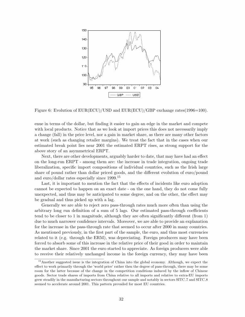
Figure 6: Evolution of EUR(ECU)/USD and EUR(ECU)/GBP exchange rates(1996=100).

enue in terms of the dollar, but finding it easier to gain an edge in the market and competewith local products. Notice that as we look at import prices this does not necessarily implya change (fall) in the price level, nor a gain in market share, as there are many other factorsat work (such as changing retailer margins). We treat the fact that in the cases when ourestimated break point lies near 2001 the estimated ERPT rises, as strong support for theabove story of an asymmetrical ERPT.

Next, there are other developments, arguably harder to date, that may have had an effecton the long-run ERPT - among them are: the increase in trade integration, ongoing tradeliberalization, specific import compositions of individual countries, such as the Irish largeshare of pound rather than dollar priced goods, and the different evolution of euro/poundand euro/dollar rates especially since 1999.15

Last, it is important to mention the fact that the effects of incidents like euro adoptioncannot be expected to happen on an exact date - on the one hand, they do not come fullyunexpected, and thus may be anticipated to some degree, and on the other, the effect maybe gradual and thus picked up with a lag.

Generally we are able to reject zero pass-through rates much more often than using thearbitrary long run definition of a sum of 5 lags. Our estimated pass-through coefficientstend to be closer to 1 in magnitude, although they are often significantly different (from 1)due to much narrower confidence intervals. Moreover, we are able to provide an explanationfor the increase in the pass-through rate that seemed to occur after 2000 in many countries.As mentioned previously, in the first part of the sample, the euro, and thus most currenciesrelated to it (e.g. through the ERM), was depreciating. Foreign producers may have beenforced to absorb some of this increase in the relative price of their good in order to maintainthe market share. Since 2001 the euro started to appreciate. As foreign producers were ableto receive their relatively unchanged income in the foreign currency, they may have been

15Another suggested issue is the integration of China into the global economy. Although, we expect theeffect to work primarily through the ’world price’ rather then the degree of pass-through, there may be someroom for the latter because of the change in the competition conditions induced by the inflow of Chinesegoods. Sector trade shares of imports from China relative to all imports and relative to extra-EU importsgrew steadily in the manufacturing sectors throughout our sample and notably in sectors SITC 7 and SITC 8seemed to accelerate around 2001. This pattern prevailed for most EU countries.

32

able to pass on a larger part of the change in the exchange rate.To summarize, in this paper, we propose a new estimate of the long-run ERPT. The

incorporation of the levels equilibrium relationship that we propose renders the empiricalestimation of ERPT more consistent with the theoretical underpinnings.

The empirical literature has been somewhat forced to look for alternative, more arbi-trary definitions of long-run ERPT, because of a failure to find a cointegrating relationshipbetween the variables. We show that proper choice of lag lengths in unit root tests, allowingfor breaks in the series and using panel methods facilitates the discovery of such an equi-librium relationship in the data, and thus improved estimation of both long and short-runERPT.

Overall, ERPT in the long run is found to be equal to one or close to one in thecommodity sectors, throughout the entire sample, while it tends to be rather lower thanone in the manufacturing, food, beverages and tobacco and chemical sectors. As there area number of reasons, such as the introduction of the euro and exchange rate developmentsthat lead us to suspect a potential change in the long run relationship, we use up-to-datepanel methods, to estimate possible break dates and changes in ERPT and account forpossible cross-section dependence.

We tend to favor the most flexible specification, i.e. the one allowing for a break inthe entire cointegrating relationship. Such a specification is more general and moreoverprovides estimates of the shift in constant that are more in line with the expected increasein competition arising out of trade integration and the introduction of the euro.

Allowing for a structural break in the relationship we find that ERPT has generallyincreased in the time period near the introduction of the euro and the change is especiallyevident in Southern European countries. This may be the effect of perceived stabilizationin the monetary regime, which led to less noise in exchange rate developments. Moreoverthe increase in ERPT in the second part of our sample may be due to specific exchange ratedevelopments (euro/dollar depreciation till 2000, and subsequent appreciation) which maysuggest asymmetrical response of the import prices. When we allow for the change in thelong run relationship, we find that, towards the second part of our sample, that is after theestimated break date, apart from Greece and perhaps a number of manufacturing sectorsin Austria, long-run ERPT was not generally substantially (in most cases not significantly)lower than 1.

Obviously in order to be able to speak more confidently of the EG long-run ERPT, wewould require a longer series, ranging both further back and beyond the date of the intro-duction of the euro. While this is the subject of on-going research, we hope we have beenable in this paper to question the basis of the empirical literature surrounding estimationof ERPT and to propose a set of alternative ideas for discussion.

References

Adolfson, M.(2001), Monetary Policy with Incomplete Exchange RatePass-Through, Sveriges Riksbank Working Paper Series No. 127.Further information in IDEAS/RePEc: http://ideas.repec.org/p/hhs/hastef/0476.html.

Bai, J. and Ng, S.(2004), A PANIC Attack on Unit Roots and Cointegra-tion, Econometrica, vol. 72, pp. 1127-1177. Further information in IDEAS/RePEc:http://ideas.repec.org/a/ecm/emetrp/v72y2004i4p1127-1177.html.

33

Banerjee, A., Marcellino M. and Osbat, C.(2004), Some Cautions on the Use of PanelMethods for Integrated Series of Macroeconomic Data, Econometrics Journal, vol. 7,pp. 322-340. Further information in IDEAS/RePEc:http://ideas.repec.org/a/ect/emjrnl/v7y2004i2p322-340.html.

Banerjee, A. and Carrion-i-Silvestre, J.(2006), Cointegration in Panel Datawith Breaks and Cross-Section Dependence, ECB Working Paper no. 591.Further information in IDEAS/RePEc:http://ideas.repec.org/p/eui/euiwps/eco2006-5.html.

Campa, J., Goldberg, L., and Gonzalez Mınguez, J.(2005), Exchange-Rate Pass-Through to Import Prices in the Euro Area, NBER working paper 11632.Further information in IDEAS/RePEc:http://ideas.repec.org/p/ebg/iesewp/d-0609.html.

Campa, J. and Gonzalez Mınguez J.(2006), Differences in Exchange Rate Pass-Through in the Euro Area, European Economic Review, vol. 50, pp. 121-145.Further information in IDEAS/RePEc:http://ideas.repec.org/a/eee/eecrev/v50y2006i1p121-145.html.

Corsetti, G., Dedola, L. and Leduc, S.(2005), DSGE Models of High Exchange-Rate Volatility and Low Pass-Through, CEPR Discussion Paper No. 5377.Further information in IDEAS/RePEc:http://ideas.repec.org/p/cpr/ceprdp/5377.html.

Corsetti, G. and Pesenti, P.(2005), International Dimensions of Optimal Mon-etary Policy, Journal of Monetary Economics, vol. 52, pp. 281-305.Further information in IDEAS/RePEc:http://ideas.repec.org/a/eee/moneco/v52y2005i2p281-305.html.

Devereux, M. and Engel, C. (2002), Exchange Rate Pass-Through, Exchange Rate Volatility,and Exchange Rate Disconnect, Journal of Monetary Economics, vol. 49, pp. 913-940.Further information in IDEAS/RePEc:http://ideas.repec.org/a/eee/moneco/v49y2002i5p913-940.html.

Devereux, M., Engel, C. and Tille, C.(2003), Exchange Rate Pass-Through and theWelfare Effects of the Euro, International Economic Review, vol. 44, pp. 223-242.Further information in IDEAS/RePEc:http://ideas.repec.org/a/ier/iecrev/v44y2003i1p223-242.html.

Engle, R. and Granger C.(1987), Co-integration and error correction: Rep-resentation, estimation, and testing, Econometrica, vol. 55, pp. 251-276.Further information in IDEAS/RePEc:http://ideas.repec.org/a/ecm/emetrp/v55y1987i2p251-76.html.

Frankel, J. , Parsley, D. and Wei S.(2005), Slow Passthrough Around the World:A New Import for Developing Countries?, NBER Working Paper, No. 11199.Further information in IDEAS/RePEc:http://ideas.repec.org/p/nbr/nberwo/11199.html.

34

Gregory, A. and Hansen, B.(1996), Residual-based Tests for Cointegration inModels with Regime Shifts, Journal of Econometrics, vol. 70, pp. 99-126.Further information in IDEAS/RePEc:http://ideas.repec.org/a/eee/econom/v70y1996i1p99-126.html.

Marazzi, M., Sheets, N., Vigfusson, R., Faust, J., Gagnon, J., Marquez,J., Martin, R., Reeve, t. and Rogers J.(2005), Exchange Rate Pass-Through to U.S. Import Prices: Some New Evidence, The FederalReserve Board International Finance Discussion Papers no. 2005-833.Further information in IDEAS/RePEc: http://ideas.repec.org/p/fip/fedgif/833.html.

Obstfeld, M.(2002), Inflation-Targeting, Exchange Rate Pass-Through and Volatil-ity, American Economic Review, Papers and Proceedings, vol. 92, pp. 102-107.Further information in IDEAS/RePEc:http://ideas.repec.org/a/aea/aecrev/v92y2002i2p102-107.html.

Pedroni, P.(1999), Critical Values for Cointegration Tests in Heterogenous Panels with Mul-tiple Regressors, Oxford Bulletin of Economics and Statistics, Special issue (1999), pp.653-670. Further information in IDEAS/RePEc:http://ideas.repec.org/a/bla/obuest/v61y1999i0p653-70.html.

Smets, F. and Wouters, R.(2002), Openness, Imperfect Exchange Rate Pass-Throughand Monetary Policy, Journal of Monetary Economics, vol. 49, pp. 947-981.Further information in IDEAS/RePEc:http://ideas.repec.org/a/eee/moneco/v49y2002i5p947-981.html.

35

Appendix A - Dataimport prices - monthly indexes of import unit values (calculated to be based on local currency) forimports originating outside the euro area.foreign prices - monthly indexes of import unit values (calculated to be based on US dollars) fromimports originating outside the euro area into the euro zone.exchange rates - index of monthly average exchange rate of local currency against the US dollar.Sources: Eurostat (COMEXT). All variables are in logs.SITC code - Industry: 0 - Food and live animals chiefly for food; 1 - Beverages and Tobacco; 2 -Crude materials, inedible, except fuels; 3 - Mineral fuels, lubricants and related materials; 4 - Animaland vegetable oils, fats and waxes; 5 - Chemicals and related products, n.e.s.; 6 - Manufactured goodsclassified chiefly by materials; 7 - Machines, transport equipment; 8 - Manufactured goods n.e.c.

• CG data set 1989-2001 - series for 1989m1-2001m3: Belgium+Luxembourg, France, Germany,Greece, Ireland, Italy, Netherlands, Portugal and Spain. Series for 1996m1-2001m3: Austriaand Finland.

• ”new” data set 1995-2005 - 1995m1-2005m3 for 10 out of 11 countries of the CG data set(Belgium+Luxembourg excluded, Austria and Finland start 1996m1, Portugal and Austriastop 2004m12)

• full panel - reduced version of 1995-2005 data set, trimmed in order to obtain a balancedpanel. Covers 1996m1-2004m12 for all 10 countries.

• full panel for CG 1989-2001 sample - 9 countries: Austria and Finland excluded, due to shortseries. Series Ireland SITC 4 and Portugal SITC 4 also excluded due to missing values.

36

Appendix B - Descriptions of tests16

Single equations with breaks - Gregory and Hansen (1996), panel cointegra-tion without cross-sectional dependence: Pedroni (1999) - without breaks andwith breaks as in Banerjee and Carrion-i-Silvestre (2006)For the purpose of describing the formal setup of the tests, let {Yi,t} be a (m× 1)-vector ofnon-stationary stochastic process with the following representation

∆xi,t = vi,t (14)yi,t = fi (t) + x′i,tδi,t + ei,t; ei,t = ρiei,t + εi,t, (15)

where Yi,t =(yi,t, x

′i,t

)′is conveniently partitioned into a scalar yi,t and the ((m− 1)× 1)-

vector xi,t, i = 1, . . . , N , t = 1, . . . , T . Let ξi,t =(εi,t, v

′i,t

)′be a random sequence assumed

to be strictly stationary and ergodic, with mean zero and finite variance. In addition,the partial sum process constructed from {ξi,t} satisfy the multivariate invariance principledefined in Phillips and Durlauf (1986). At this stage and in order to set the analysis in asimplified framework, let us assume that {vi,t} and {εi,t} are independent.

The general functional form for the deterministic term f (t) is given by:

fi (t) = µi + βit + θiDUi,t + γiDT ∗i,t, (16)

where

DUi,t ={

0 t ≤ Tbi

1 t > Tbi; DT ∗i,t =

{0 t ≤ Tbi

(t− Tbi) t > Tbi, (17)

with Tbi = λiT , λi ∈ Λ, where Λ is a closed subset of (0, 1), for the applications consideredΛ is given by [0.15, 0.85], denoting the time of the break for the i-th unit, i = 1, . . . , N .Note also that the cointegrating vector is specified as a function of time so that

δi,t ={

δi,1 t ≤ Tbi

δi,2 t > Tbi. (18)

Using these elements, Banerjee and Carrion-i-Silvestre (2006) propose up to six differentmodel specifications, of which for the purpose of this paper we will review two:

• Model 1. Constant term with a change in level but stable cointegrating vector:

yi,t = µi + θiDUi,t + x′i,tδi + ei,t (19)

• Model 4. Constant term with change in both level and cointegrating vector:

yi,t = µi + θiDUi,t + x′i,tδi,t + ei,t (20)

Using any one of these specifications the authors propose testing the null hypothesis ofno cointegration against the alternative hypothesis of cointegration (with break) using theADF test statistic applied to the residuals of the cointegration regression as in EG and GH

16This Appendix is an extract from Banerjee and Carrion-i-Silvestre (2006). For more details, includingsetup, derivations, asymptotic properties and finite sample simulations we refer the reader to the originalpapers.

37

but in the panel data framework developed in Pedroni (1999, 2004). In fact, GH proposeboth of the specifications given by models 1 and 4 above.

The Banerjee and Carrion-i-Silverstre (2006) proposal starts by following Gregory andHansen (1996), to the OLS estimation of one of the models given above (in our case (19)and (20)) and run the following ADF type-regression equation on the estimated residuals(ei,t (λi)):

∆ei,t (λi) = ρiei,t−1 (λi) +k∑

j=1

φi,j∆ei,t−j (λi) + εi,t. (21)

The notation used refers to the break fraction (λi) parameter, which (if it exists) is inmost cases unknown. In order to get rid of the dependence of the statistics on the breakfraction parameter, Gregory and Hansen (1996) suggest estimating the models given abovefor all possible break dates, subject to trimming, obtaining the estimated OLS residualsand computing the corresponding ADF statistic.With the sequence of ADF statistics in hand, one can also estimate the break point for eachunit as the date that minimizes the sequence of individual ADF test statistics – either the t-

ratio, tρi (λi), or the normalized bias, computed as T ρi (λi) = T ρi

(1− φi,1 − · · · − φi,k

)−1

– see Hamilton (1994), pp. 523. Note that the estimation of the break point Tbi is conductedas

Tbi = arg minλi∈Λ

tρi(λi) ; Tbi = arg min

λi∈ΛT ρi (λi) , (22)

∀i = 1, . . . , N . At this point Gregory and Hansen (1996) test the null hypothesis foreach unit. Gregory and Hansen (1996) derive the limiting distribution of tρi

(λi

)=

infλi∈Λ tρi (λi) and T ρi

(λi

)= infλi∈Λ T ρi (λi), which are shown not to depend on the

break fraction parameter. Specifically, Gregory and Hansen (1996) show that T ρi

(λi

)⇒

infλi∈Λ

∫ 10 Q (λi, s) dQ (λi, s)

/ ∫ 10 Q (λi, s)

2 ds, and tρi

(λi

)⇒ infλi∈Λ

∫ 10 Q (λi, s) dQ (λi, s)

/

[∫ 10 Q (λi, s)

2 dr(1 + % (λi)

′D (λi) % (λi))]1/2

, where ⇒ denotes weak convergence, Q (λi, s)and % (λi) are functions of Brownian motions and the deterministic component, and D (λi)depends on the model – see the Theorem in Gregory and Hansen (1996) for further details.

Banerjee and Carrion-i-Silvestre (2006) propose combining the unit-specific informationin a panel data statistic.

The panel statistics on which they focus in order to test the null hypothesis are given bythe ZρNT

and ZtNTtests in Pedroni (1999, 2004), which can be thought as analogous to the

residual-based tests in EG. These test statistics are defined by pooling the individual ADFtests, so that they belong to the class of between-dimension test statistics. Specifically, theyare computed as:

N−1/2ZρNT

(λ)

= N−1/2N∑

i=1

T ρi

(λi

)(23)

N−1/2ZtNT

(λ)

= N−1/2N∑

i=1

tρi

(λi

). (24)

where ρi

(λi

)and tρi

(λi

)are the estimated coefficient and associated t-ratio from (21)

38

and

λ =(λ1, λ2, . . . , λi, . . . , λN

)′(25)

is the vector of estimated break fractions.Note that this framework allows for a high degree of heterogeneity since the cointegrating

vector, the short run dynamics and the break point estimate might differ among units. Theuse of the panel data cointegration test aims to increase the power of the statistical inferencewhen testing the null hypothesis of no cointegration, but some heterogeneity is preservedwhen conducting the estimation of the parameters individually.

Following Pedroni (1999), the panel test statistics are shown to converge to standardNormal distributions once they have been properly standardized.

Panel cointegration with cross-sectional dependence: Banerjee and Carrion-i-Silvestre (2006)

The setup above extended static-regression based tests for cointegration to allow forstructural breaks in the components of the regression (that is a break in the constant, as inequation (12) and a break in the constant and slope, as in equation (13)). The underlyingassumption was that panel units are cross-sectionally independent, which is quite rarely thecase in economic applications. The extended approach in Banerjee and Carrion-i-Silvestre(2006) models cross-sectional dependence using common factors such as in Bai and Ng(2004). The test described here is for a common (across all the units), known structuralbreak point and we refer the reader to the original paper for details on the estimationstrategy in the case of unknown, unit-specific breaks, which is used in our paper.The underlying model is given in the following structural form:

yi,t = fi (t) + x′i,tδi,t + ui,t (26)ui,t = F ′

tπi + ei,t (27)(I − L) Ft = C (L) wt (28)

(1− ρiL) ei,t = Hi (L) εi,t (29)(I − L) xi,t = Gi (L) vi,t, (30)

t = 1, . . . , T , i = 1, . . . , N , where C (L) =∑∞

j=0 CjLj , and fi (t) denotes the deterministic

component (which may be broken as in (16) above), Ft denotes a (r × 1)-vector containingthe common factors, with πi the vector of loadings. Despite the operator (1−L) in equation(28), Ft does not have to be I(1). In fact, Ft can be I(0), I(1), or a combination of both,depending on the rank of C(1). If C(1) = 0, then Ft is I(0). If C(1) is of full rank, theneach component of Ft is I(1). If C(1) 6= 0, but not full rank, then some components of Ft

are I(1) and some are I(0). Our analysis is based on the same set of assumptions in Bai andNg (2004), and Bai and Carrion-i-Silvestre (2005). With a number of assumptions on theloadings and error terms from the above equations we one can continue the estimation ofcommon factors as is done in Bai and Ng (2004). We need to compute the first differences:

∆yi,t = ∆fi (t) + ∆x′i,tδi,t + ∆Ftπi + ∆ei,t, (31)

39

and take the orthogonal projections:

Mi∆yi = Mi∆Fπi + Mi∆ei (32)= fπi + zi, (33)

with Mi = I −∆xdi

(∆xd′

i ∆xdi

)−1 ∆xd′i being the idempotent matrix, and f = Mi∆F and

zi = Mi∆ei. The superscript d in ∆xdi indicates that there are deterministic elements.

The estimation of the common factors and factor loadings can be done as in Bai andNg (2004) using principal components. Specifically, the estimated principal component off = (f2, f3, . . . , fT ), denoted as f , is

√T − 1 times the r eigenvectors corresponding to the

first r largest eigenvalues of the (T − 1)× (T − 1) matrix y∗y∗′, where y∗i = Mi∆yi. Underthe normalization f f ′/ (T − 1) = Ir, the estimated loading matrix is Π = f ′y∗/ (T − 1).Therefore, the estimated residuals are defined as

zi,t = y∗i,t − ftπi. (34)

One can recover the idiosyncratic disturbance terms through cumulation, i.e. ei,t =∑tj=2 zi,j , and test the unit root hypothesis (αi,0 = 0) using the ADF regression equation

∆ei,t (λ) = αi,0ei,t−1 (λ) +k∑

j=1

αi,j∆ei,t−j (λ) + εi,t. (35)

We denote by ADF ce (i) the pseudo t-ratio ADF statistics for testing αi,0 = 0 in (35).

As in (24) the individual ADF statistics ADF ce (i) for the idiosyncratic disturbance terms

can be pooled to define a panel data cointegration test. Thus, one can define

N−1/2ZetNT

−Θe2

√N ⇒ N (0, Ψe

2) , (36)

where the superscript e denotes the idiosyncratic disturbance. The moments Θe2 and Ψe

2

are the same as the ones for the statistics in Bai and Ng (2004), where these do not dependon the break fraction λ.

40