Exchange Rate and Wage Adjustment:

a Firm-Level Investigation∗

Francesco Nucci

Sapienza Universita di Roma

Alberto Franco Pozzolo

Universita del Molise

September 26, 2011

Abstract

In this paper we rely on a representative panel of manufacturing firms and estimate theimplications for firm-level wages of changes in the permanent component of the exchange rate.Similarly to the response of employment and hours documented in Nucci and Pozzolo (2010),the direction and size of wage adjustment is shaped by the external orientation of each firm onboth the sale and cost side of the balance sheet. Through the revenue side, wages are shownto rise after a currency depreciation and the effect is estimated to be larger the higher is thefirm’s exposure to sales from exports. On the contrary, a depreciation induces a cut in firm’swages through the expenditure side of the balance sheet and the effect is larger the higher isthe incidence of imported inputs on total production costs. We show that, for a given degreeof firm’s external orientation, the sensitivity of wages to exchange rate swings is larger for firmswith a lower market power. We also document that other transmission channels provide a degreeof difference in shaping the effect of exchange rates on wages. These include: a) the degree ofsectoral import penetration in the domestic market; b) the extent of inputs substitutability infirm’s production; c) the percentage of newly hired workers in each firm in a given year and d)the composition of the firm’s labor force by type.JEL classifications: E24; F16; F31.Keywords: Exchange Rate; Wages; Firms’ Foreign Exposure.

∗This project was begun while Alberto Pozzolo was with the Research Department of the Bank of Italy. We thank

seminar participants at the 2011 IEA Conference in Beijing and the XIX Tor Vergata Conference on Money, Banking

and Finance (Rome) for useful discussions. E-mail addresses: francesco.nucci@uniroma1.it; pozzolo@unimol.it.

1

1 Introduction

A substantial body of empirical literature uncovers non-negligible effects of exchange rate move-ments on the real economy. Some contributions, for example, document that currency swingssignificantly affect firm’s investment (Campa and Goldberg, 1999 and Nucci and Pozzolo, 2001)as well as employment and hours (Nucci and Pozzolo, 2010). As for these labor market effects,however, the latter finding contrasts with previous evidence by Campa and Goldberg (2001) on aweak employment response to exchange rates coupled with significant implications for real wages.Differently from Campa and Goldberg (hereafter, CG) and most other studies in this area of lit-erature, Nucci and Pozzolo (hereafter, NP) use firm- rather than industry-level data and providearguments for why the level of disaggregation of the data may affect the estimated impact on em-ployment to a considerable extent. The present paper relies on the same microeconomic data andseeks to investigate how real wages at the firm level responds to exchange rate variations, thuscomplementing the NP (2010)’s analysis along a parallel dimension.

Assessing the consequences of exchange rate movements for the earnings of workers is indeed an openquestion. On the one hand, a group of contributions, focusing on aggregate data at the industrylevel, uncover a significant wage responsiveness to exchange rate oscillations. In particular, Revenga(1992) shows that changes in import prices induced by exchange rate swings do affect real wagein U.S. Manufacturing. Using data disaggregated by states and by industries, Goldberg and Tracy(2000) report statistically significant estimates of the earnings elasticities with respect to exchangerate, also providing evidence of a pattern of regional differences in their values. More recently, CG(2001) document a significant incidence of exchange rates on wages that varies across industriesdepending on their trade orientation and competitive structure.

On the other hand, however, a study on microeconomic data by Goldberg and Tracy (2003) findsthat the overall wage effect of currency movements is in fact modest, although it can be sizeable forspecific groups of workers. In their paper the authors focus on information on individual workersand analyze how the wage sensitivity to exchange rate is shaped by workers’ specific characteristicssuch as those related to educational attainment and experience.1

1A notable feature of analyzing data on individual workers is that it allows to track the wage implications of a

worker’s job transition, which can be sizeable (see Kletzer, 1999). On this respect, Kletzer (1999) and Goldberg and

Tracy (2003) show that increasing foreign competition as well as exchange rate changes account for a modest share

of job displacement. On the other hand, however, job changing does affect the sensitivity of wages to exchange rate

2

Information on individual workers definitely provides a useful dimension for the analysis, as itallows to appraise which type of workers experience the largest wage adjustment (if any) afteran exchange rate shock. We argue, however, that individual firm characteristics are of particularrelevance in shaping the implications for wages of exchange rate fluctuations. In particular, becauseof the large heterogeneity across firms along several dimensions, even within narrowly definedindustries, the firm-specific effects of exchange rate on wages can be to some extent washed out in theaggregation process. A very important dimension of such heterogeneity pertains to the internationaltrade exposure of each individual firm and, indeed, a large body of literature emphasizes profounddifferences across firms in their degree of international orientation on both the export and importedinputs side (see Bernard et al, 2007). This calls for an investigation on data at the firm level. Inparticular, we are able to estimate a specific, time-varying responsiveness of the (average) wageto exchange rate for each individual firm and in doing so we allow for a number of transmissionchannels of the currency shock to the wages whose relevance varies from firm to firm.

In order to provide motivation for the empirical analysis, following NP (2001; 2010) and CG (1999;2001) we rely on a theoretical model that pins down a number of mechanisms through whichexchange rate changes influence the wages set by the firm. In particular, exchange rate is shown toaffect the firm’s profitability and thereby its equilibrium outcomes for wages and employment. Thus,in the aftermath of a currency depreciation, for example, there is a positive wage and employmentadjustment through the revenue side of the income account, whose size increases with the extentof firm’s exposure to foreign product markets. Through the cost side, conversely, a depreciationtends to reduce wages (and employment) in the firm and the effect is stronger the more a firm relieson imported intermediate inputs for its production. Another prediction of the theoretical model,which is testable with our data, is that, for a given level of firm’s external orientation, the degreeof wage sensitivity to exchange rate is influenced by the market power of the firm. In particular,the impact on wages is found to be more pronounced the lower is the firm’s pricing power in itsdestination markets (see CG, 2001). We also investigate the empirical relevance of other features inshaping the responsiveness of wages to exchange rate at the firm level. A relevant aspect deals withthe degree of competitive pressure exerted by foreign producers in the firm’s domestic market. Inline with NP (2010), we therefore investigate on our firm data whether differences across industriesin the degree of import penetration are conducive to diverging patterns of the responses of wage tocurrency shocks. In doing so, we combine firm-level information on the exposure of the firm’s saleson the domestic product markets with data on import penetration in the industry to which the firmbelongs. We find that a currency appreciation, for example, by reducing firm’s competitiveness in

through the impact of currency swings on the size of the wage adjustment after a job transition (Goldberg and Tracy,

2003).

3

the domestic market, reduces profitability and thereby the equilibrium wages through the domesticrevenue channel and this effect is found to be stronger the higher is the extent of import penetrationon the one side and the larger is the degree of firm’s orientation to the domestic product marketson the other. We also investigate another possible source of specificity in the wage sensitivity toexchange rate by examining whether the wage responsiveness through the cost side varies acrossfirms in light of differences in their degree of substitutability in production between imported anddomestically produced intermediate inputs.

Moreover, in shaping the impact of exchange rate movements on the wages set by the firm a relevantaspect deals with the share of newly hired workers in the firm in a given year. In particular, weconsider the hiring rate for each firm and ask ourselves whether two firms with a different percentageof newly hired employees in a given year but which are otherwise identical along all dimensions(e.g. international exposure) exhibit a different sensitivity of the (average) wage to exchange rateshocks. We find that this sensitivity is indeed of a larger size for the firm with the higher hiringrate, as we estimate for it a stronger wage responsiveness to a currency shock along both thetwo transmission channels related to the firm’s foreign exposure (the one though exports and theone through imported inputs). Arguably, this result seems to complement the one obtained onemployees data by Goldberg and Tracy (2003), who detect a significant effect of exchange rate onthe amount of the worker’s wage adjustment associated with a transition from a job to another.

Finally, whilst our data do not allow to control for individual worker characteristics such as theskill level, we do have, however, time-varying information for each firm on the composition of itsworkforce by type. We therefore examine whether the overall exchange rate elasticity of wagestends to vary in coincidence with a different incidence in the firm of the blue-collar employees(vis-a-vis the white-collars).

We organize the remainder of the paper as follows: section 2 presents the theoretical relationshipsthat guide our empirical analysis and provide motivation for it. Section 3 describes the data, theempirical specification and the estimation methodology. In section 4 we report the baseline empiri-cal results and in section 5 we investigate additional features that provide further characterizationsof the wage responsiveness to exchange rate swings. Finally, section 6 concludes.

4

2 Theoretical framework

2.1 The Model

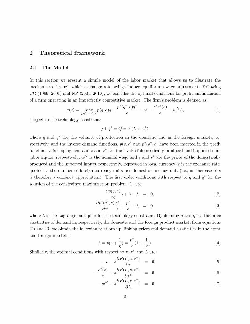
In this section we present a simple model of the labor market that allows us to illustrate themechanisms through which exchange rate swings induce equilibrium wage adjustment. FollowingCG (1999; 2001) and NP (2001; 2010), we consider the optimal conditions for profit maximizationof a firm operating in an imperfectly competitive market. The firm’s problem is defined as:

π(e) = maxq,q∗,z,z∗,L

p(q, e)q +p∗(q∗, e)q∗

e− zs− z∗s∗(e)

e− wNL, (1)

subject to the technology constraint:

q + q∗ = Q = F (L, z, z∗).

where q and q∗ are the volumes of production in the domestic and in the foreign markets, re-spectively, and the inverse demand functions, p(q, e) and p∗(q∗, e) have been inserted in the profitfunction. L is employment and z and z∗ are the levels of domestically produced and imported non-labor inputs, respectively; wN is the nominal wage and s and s∗ are the prices of the domesticallyproduced and the imported inputs, respectively, expressed in local currency; e is the exchange rate,quoted as the number of foreign currency units per domestic currency unit (i.e., an increase of eis therefore a currency appreciation). The first order conditions with respect to q and q∗ for thesolution of the constrained maximization problem (1) are:

∂p(q, e)∂q

q + p− λ = 0, (2)

∂p∗(q∗, e)∂q∗

q∗

e+p∗

e− λ = 0. (3)

where λ is the Lagrange multiplier for the technology constraint. By defining η and η∗ as the priceelasticities of demand in, respectively, the domestic and the foreign product market, from equations(2) and (3) we obtain the following relationship, linking prices and demand elasticities in the homeand foreign markets:

λ = p(1 +1η

) =p∗

e(1 +

1η∗

). (4)

Similarly, the optimal conditions with respect to z, z∗ and L are:

−s+ λ∂F (L, z, z∗)

∂z= 0, (5)

−s∗(e)e

+ λ∂F (L, z, z∗)

∂z∗= 0, (6)

−wN + λ∂F (L, z, z∗)

∂L= 0. (7)

5

By combining Eq. (4) with the above three equations, the following equilibrium conditions arederived, equating the marginal revenue product of each input to its marginal cost (see NP, 2011;2010):

∂F (L, z, z∗)∂z

=s

p(1 + 1η ), (8)

∂F (L, z, z∗)∂z∗

=s∗(e)

p∗(1 + 1η∗ )

, (9)

∂F (L, z, z∗)∂L

=wN

p(1 + 1η ). (10)

If we assume that technology, F (·), is described by a constant return to scale production function,we apply Euler’s theorem and express total output as follows:

Q = F (L, z, z∗) =∂F (L, z, z∗)

∂LL+

∂F (L, z, z∗)∂z

z +∂F (L, z, z∗)

∂z∗z∗. (11)

By defining 1µ = (1+ 1

η ) and 1µ∗ = (1+ 1

η∗ ) as the reciprocals of the mark-up ratios set, respectively,in the domestic and foreign product markets, and substituting Eqs. (8) through (10) into Eq. (11),simple algebraic manipulations yield the following equilibrium condition (see CG, 2001 and NP,2010):

wNL =pq

µ+p∗q∗

eµ∗− (sz +

s∗z∗

e). (12)

The above expression characterizes firm’s optimal labor demand in the absence of adjustment costs.By applying the logarithmic transformation to it and denoting L̃ as the optimal demand in theabsence of adjustment costs yield

lnwN = ln[pq

µ+p∗q∗

eµ∗− (sz +

s∗z∗

e)]− ln L̃. (13)

Let us allow for adjustment costs in hiring and firing workers and postulate the following partialadjustment equation for labor demand

lnLt = ϕ lnLt−1 + (1− ϕ) ln L̃t; (14)

it dictates that optimal labor demand in period t depends on the previous period’s level, t− 1, andon the optimal current level in the absence of adjustment costs, lnL̃t. ϕ is a parameters governingthe speed of adjustment (see NP, 2010).

6

Combining Eqs. (13) and (14) and using the time subscripts yield the following expression

lnwNt = ln[ptqtµt

+p∗t q∗t

etµ∗t− (stzt +

s∗t z∗t

et)]− 1

1− ϕ(lnLt − ϕ lnLt−1). (15)

In order to fully characterize the labor market, we need to introduce a labor supply schedule.Following CG (2001) and NP (2010), we assume that labor supply obeys the following relationship:

lnLt = a0 + a1 lnwt + a2 lnYt (16)

where Y is a measure of aggregate demand and w is the real wage, i.e. the nominal wage, wNtdeflated by an aggregate price index, P . By equating labor demand (Eq. 15) and labor supply(Eq. 16), simple manipulations yield

lnwt = A(1−ϕ){ln[p(qt, et) · qt

µ+p∗(q∗t , et) · q∗t

etµ∗−(stzt+

s∗(et)z∗tet

)]−lnP t}+Aϕ lnLt−1−A(a0+a2 lnYt),

(17)

where A = 11−ϕ+a1

. After differentiating the above equation with respect to the exchange rate,simple algebraic transformations yield the following expression for the elasticity of real wages, w,with respect to exchange rate, e

d lnwtd ln et

=1µβ[−χ(1− ηp∗,e) + (1− χ)ηp,e + α(1− ηs∗,e)]A(1− ϕ), (18)

where χ ∈ [0, 1] is the share of sales in foreign markets over total sales and (1 − χ) ∈ [0, 1] is theshare of sales in domestic market over total sales; α ∈ [0, 1] is the share of production costs onimported inputs in total costs; ηp,e ∈ [−1, 0] and ηp∗,e ∈ [0, 1] are the elasticities of, respectively,domestic and foreign prices with respect to the exchange rate (i.e., the pass-through elasticities);ηs∗,e ∈ [0, 1] is the elasticity of foreign input prices with respect to the exchange rate. β is the shareof labor costs over total revenues. In deriving the above expression we have assumed for simplicitythat there is no distinction between the mark-up set in the domestic market, µ, and the one in theforeign product markets, µ∗. In both cases we have used µ, which can be interpreted as the averagevalue of the destination-specific mark-up ratios (see NP, 2010). Moreover, in obtaining Eq. (18)we have used the fact that, under constant returns to scale, total revenues can be expressed as theproduct of production costs (the wage bill plus intermediate input expenditure) and the mark-upratio, µ.

7

Eq. (18) represents a useful theoretical background for our empirical analysis, providing a varietyof testable implications. The following section discusses in more detail the number of channels,explicitly identified in our theoretical model, through which exchange rate movements affect theequilibrium outcome for wages.

2.2 The Channels of Transmission of Currency Swings to Wages

Equation (18) predicts that exchange rate swings affect wage adjustments. In particular, if wefocus on the revenue side of the firm’s balance sheet a currency depreciation (a reduction of et) hasa positive effect on the firm’s marginal revenue product of labor and thereby on the equilibriumoutcome for real wages, as is shown by the sum of the first two terms inside brackets in Eq. (18),−χ(1 − ηp∗,e) + (1 − χ)ηp,e, which is non-positive. In particular, a depreciation is predicted toexert a positive effect on wages along both the foreign and domestic sales channels. By contrast,a currency depreciation negatively affects, through the cost side of the balance sheet, the marginalrevenue product of labor and thereby real wages. Indeed, the term α(1−ηs∗,e) inside brackets in Eq.(18) is non-negative. Very importantly, the extent of these adjustments depends on the externalorientation of the firm towards international product markets. On the export side, the positiveeffect on wages of an exchange rate depreciation is larger the higher is the share of foreign sales ontotal sales, χ, i.e. the more a firm is exposed to foreign markets through the export of its products.On the revenue side as a whole, i.e. including both domestic and foreign sales, the positive effect onwages on a currency depreciation is also amplified as the export share of sales, χ, becomes larger,but this prediction holds true only if the following condition is met: |ηp,e|+ηp∗,e < 1, i.e. if the sumof the exchange rate pass-through elasticities (their absolute value) is less than one (NP, 2010). Onthe expenditure side, conversely, the size of the negative effect on wages of a currency depreciationdepends on the extent of firm’s reliance upon imported inputs. This type of exposure is captured inEq. (18) by α, the share of expenditure on imported inputs on total costs: the larger is this share,the more pronounced the negative implications for wages of a depreciation through this channel ofexposure (see CG, 1999; 2001 and NP 2001; 2010).

The theoretical framework illustrated in the previous section highlights other important featuresthat shape the response of wage to exchange rate swings. First, the firm’s degree of market power, asmeasured by the firm’s mark-up ratio, µ, does enters Eq. (18) and the prediction is that, everythingelse being identical for two firms (e.g., type of international exposure and pass-through elasticities),the one with a lower degree of monopoly power tends to exhibit a more sizeable (absolute valueof the) elasticity of wages to exchange rate. Indeed, firms with a lower market power tend to beless capable to absorb currency shocks so that the impact on wages is relatively more pronounced.

8

To see this, recall that an exchange rate depreciation (e.g. a decrease of e) drives down the exportprice in the foreign currency by an amount that depends on the pass-through elasticity, ηp∗,e. Thisprice decline therefore yields an increase of foreign demand, q∗, and thereby of profitability andwages, which is larger the higher is the price elasticity of foreign demand, η∗. Given the negativerelationship between the firm’s mark-up ratio and the price elasticity of demand, the sensitivity ofwage to currency swings is indeed magnified when the firm’s market power is relatively low.

Moreover, another prediction of the model (again see Eq. 18) is that the exchange rate pass-through elasticities contribute to shape the adjustment of wage in response to currency shocks.The exchange rate elasticity of prices set by the firm in the destination market’s currency, ηp∗,eranges from zero (no pass-through) to one (complete pass-through). From Eq. (18) we note that,for a given level of external orientation on the export side, χ, the smaller is the elasticity of exchangerate pass-through to foreign prices, ηp∗,e, the larger is the (absolute value of the) wage response toa shift in et. Importantly, a number of contributions show that this exchange rate pass-throughelasticity does depend on market structure and in particular on the extent to which firms’ productsare differentiated and the substitution among different variants is large (Yang, 1997). These studiesinclude Dornbusch (1987) and Knetter (1993) and show that the pass-through tends to be low if thedegree of competition in the foreign markets is high. Therefore, in the limiting case of a perfectlycompetitive foreign destination market, the firm is a price taker and the pass-through elasticitywould be zero. Thus, the prediction through this channel contributes to reinforce the previousconclusion that the lower is the firm’s pricing power the higher is the exchange rate sensitivity ofwages.

If we focus on firm’s competition in the domestic market, we have established that a currencydepreciation, by making foreign products more expensive, rises the competitiveness of domesticfirms in the home market, thus increasing their sales and thereby their profitability and wages.Eq. (18) predicts that the exchange rate pass-through elasticity of firm’s prices in the domesticmarket, ηp,e, plays an important role in shaping this effect. The values of this domestic pass-throughelasticity range from minus one (complete pass-through) to zero (no pass-through), and again itdepends on market structure. Specifically, the elasticity is (in absolute value) a decreasing functionof the firm’s monopoly power in the home market. In the limiting case of a perfectly competitivedomestic destination market, where the domestic firm is a price taker, a currency appreciationmust be rebated by a one-to-one firm’s own price cut (a pass-through elasticity equal to minusone). Thus, a currency appreciation induces a reduction in the value of domestic sales, profitabilityand wages and the lower the firm’s market power the larger this decline turns to be. The intuition isthat the higher the competitive pressure exerted by foreign producers, the more responsive domestic

9

sales, profitability and wages are in the aftermath of a currency shift. Indeed the domestic pass-through elasticity reflects the degree of this competitive pressure from foreign producers and isoften assumed to be proportional to the degree of import penetration in the domestic market (seee.g. Dornsbusch, 1987 and CG, 2001).

Market structure also affects the effects through the expenditure side of the balance sheet. Indeed,the increase of wages after an exchange rate appreciation taking place through a reduction in theexpenditure for imported inputs depends on the extent of competition in the market for intermediateinputs. Indeed, Eq. (18) establishes that the effect of exchange rate on wage adjustment is largerthe smaller the pass-through elasticity of foreign input prices to the exchange rate, ηs∗,e. The latterranges from zero (no pass-through) to one (complete pass-through).

The theoretical framework allows us to uncover a number of testable implications on the channelsof transmission of exchange rate swings to wage adjustments. These theoretical predictions aresummarized by Eq. (18) and lend themselves to the empirical scrutiny to which we now turn. Indoing so, we first present the firm-level panel data that we use.

3 The Data and Regression Specification

3.1 The Data

In the empirical investigation the microeconomic data that are used are the the same as thoseof NP (2010). They are drawn from two different statistical sources. The first one is the Bankof Italy’s Survey of Investment in Italian Manufacturing (SIM) carried out at the beginning ofevery year since 1984 on a representative sample of over 1,000 firms stratified by industry, firmsize and location. The data are of extremely high quality also for the professional expertise of theinterviewers, who are officials of the Bank of Italy establishing long-term relationships with thefirms’ managers. In order to ensure the quality standard of data, only medium-large firms, definedas those with more than 50 employees, are included in the Survey. We used SIM to gather firm-levelinformation on total revenues and revenues from exporting, employment and hours worked.

The second data source of firm-level data is the Company Accounts Data Service reports, a databasemaintained by a consortium of the Bank of Italy and a pool of banks, collecting information frombalance sheets and income statements of a sample of about 40,000 Italian firms. The detailedinformation from the annual accounts are reclassified to ensure comparability across firms. Thisdatabase provides us with firm level information on labor compensation, intermediate input ex-

10

penditure, value added and gross output. Data from the two sources are merged to constructan unbalanced panel of slightly fewer than 2,400 firms. As in NP (2010), the data used for es-timation covers the period 1984-1998, the one antecedent to the introduction of the Euro. Thisperiod was characterized by pronounced swings of the Italian currency coupled with a high degreeof international exposure of Italian firms.

We compute wages at the firm-level by considering both firm’s labor costs per employee and firm’slabor costs per hour. These measures of labor compensation are expressed in real terms by usingthe GDP deflator. The number of firm’s employees is the average value within each year. Theempirical counterpart of the two key variables on the firm’s international exposure, χ and α, arecalculated at the firm level for each year as follows: χit is the export share of sales of firm i in yeart computed using data from SIM. In order to derive αit, the share of imported inputs in total inputpurchases of firm i in year t, we had to augment firm-level information from the two statisticalsources with additional information as the value of firm’s expenditure on imported inputs is notavailable. As documented in NP (2001 and 2010), we do so by relying on the 44-industry input-output table of 1992 for the Italian economy. in particular, we extract for each industry j thevalues of both imported intermediate inputs and total intermediate inputs (domestically producedand imported). Then, by using time series on import demand and production for each industry, weupdated backward and forward the values of input purchases from the input-output table that referto one year only. Lastly, we computed the share of costs on imported inputs in total input purchases

as αit =

(IMjtTEjt

)TEit

TEit+LCit, where IMjt is the value of intermediate inputs imported by industry j (the

industry to which firm i belongs), TEit and TEjt are the values of total expenditure for intermediateinputs of, respectively, firm i and industry j, and LCit is labor costs of firm i.

In order to provide a time-varying measure of firm’s market power we follow the approach developedby Domowitz et al. (1986) and compute a firm’s index of mark-up as the ratio of the firm’s valueadded net of labor compensation to the value of firm’s total production. Ideally, we would usedistinct destination-specific mark-up ratios, for example in the home and the foreign markets.Since our data do not allow to derive them we construct, for each year, a firm’s average measureof market power.

For measuring exchange rate, we separately use both the export and import real effective exchangerates of the Italian lira constructed by considering 24 different bilateral exchange rates. Bothreal exchange rates are computed using producer price indexes (see Banca d’Italia, 1998). In theempirical analysis, we use the permanent component of exchange rate variations which has beenderived by applying the Beveridge and Nelson (1981) procedure that decomposes a non-stationary

11

series into its permanent and transitory components (see NP, 2010 for details). Figure 1 shows thetime profile of the monthly data on import and export real exchange rates in the period analyzedwith an increase of the exchange rates amounting to a real appreciation. While they exhibit a verysimilar pattern, some differences emerge in the mid-eighties and at the beginning of the nineties.

3.2 The Econometric Specification

In assessing on empirical grounds the wage response to exchange rate fluctuations we rely on abaseline equation which has the following specification

∆wit = β0 + β1χit−1∆peert + β2αit−1∆pmert + β3χit−1 + β4αit−1+

+ β5∆sit−1 + β6MKUPit−1 + β7∆lit−1 + b′Zit + λi + uit, (19)

where lower-case letters denote the logarithmic transformation of the variable; Wit is the averagelabor compensation in real terms paid by firm i at time t and we alternatively use the real laborcompensation per employees and the one per hour. Sit is the value of real sales and PEERt andPMERt are the permanent components of, respectively, export and import real effective exchangerates, defined so that an increase in the exchange rate is an appreciation. MKUPit is an indexof firms’ market power. Lit is the amount of labor input and we alternatively measure it as thenumber of employees and the number of total hours. Zit is a vector of dummy variables controllingfor the different years, industries, sizes and geographic locations in which each firm operates. Theempirical specification is in first-differences in light of the non-stationarity of the exchange ratetime series.

While the dynamic Eq. (19) is a reduced form, it can be seen as the empirical counterpart of Eq.(18) and allows us to test a number of theoretical implications of the model. The key variablesfor characterizing the wage adjustment in response to currency swings are 1) χit−1 · ∆peert, theinteraction term of the export share of sales lagged by one period with the export exchange ratevariation; and 2) αit−1·∆pmert, the interaction term of the lagged share of expenditure for importedinputs in total purchases with the import exchange rate variation. The advantage of this approachis that the estimated sensitivity of wages to currency movements varies across firms and over timedepending on the evolving external orientation of each specific firm on both the revenue and costside (see CG, 2001 and NP, 2010). In other words, the empirical framework (19) allows us toderive a time-varying firm specific estimated response of firms’ labor compensation to exchange

12

rate oscillations. Of course, the export share of sales and the share of imported inputs are alsoinserted in the specification as single regressors in isolation.

The specification includes the lagged value of change in employment (or hours) in order to controlfor the adjustment lags that typically characterizes the labor market. In order to control for demandconditions, we include in the equation the lagged value of changes in the firms’ real sales; we alsoinclude the lagged value of the mark-up ratio to control for the effect of marginal profitabilityon wages that is independent of exchange rate developments. The dummy variables included inthe equation comprise the year dummies that capture the time-varying effects on wages commonto all firms. The specification also includes fixed effects, λi, controlling for individual firm latentheterogeneity; uit are the disturbance terms for which we assume that E(uit) = E(uituis) = 0, forall t 6= s.

As in NP (2001 and 2010), the methodology used for estimation is the generalized method ofmoments (GMM) estimator for dynamic panel data model, which was shown to be efficient withinthe class of instrumental variable estimators (Arellano and Bond, 1991). Indeed, since in Eq. (19)the lagged values of the mark-up ratio and of change in employment (hours) and sales are likelyto be correlated with the firm-specific fixed effects, λi, this endogeneity of regressors would causeinconsistency of the parameters estimated with standard panel methods while the GMM estimatorwould ensures their consistency. Specifically, following Arellano and Bover (1995) and Blundell andBond (2000), we rely on the system GMM panel estimator which augments the Arellano and Bond(1991) estimator by building a system of two equations: the original equation and a transformedone. As in Arellano and Bond (1991), in the transformed equation a variety of instruments inlevels can be used. However, under the novel approach a further assumption is made: that firstdifferencing the instrumenting variables in the original equation makes them uncorrelated with fixedeffects. This allows us to exploit an even larger number of orthogonality conditions than before,by resorting to a larger instrument set. In the estimation we utilize as GMM-type of instrumentsthe lagged values of real sales, employment (or hours) and of the mark-up dated period t-2 andearlier. The validity of our specification is ascertained by conducting: a) the Hansen test of over-identifying restrictions, which seeks to verify the orthogonality between instrumental variables andthe disturbance terms and b) the Arellano-Bond test for second-order serial correlation of residualsof the transformed equation. We now turn to present and discuss the estimation results.

13

4 Empirical Results

4.1 The Baseline Specification

The results from estimating Eq. (19) are presented in table 1. The effect of exchange rate fluc-tuations on labor compensation set by the firms is statistically significant and this holds true byconsidering both the compensation per employee (column 1) and the compensation per hour (col-umn 2). The estimated coefficients on the two interaction terms, capturing the effect of currencyswings on wages through, respectively, the foreign sale and the imported intermediate inputs chan-nels have the expected sign and are statistically significant. For example, if we focus on the responseof real wages per employee (see column 1) the estimated coefficient of χit−1 ·∆peert is −0.722 witha standard error of 0.140 while the estimated coefficient of αit−1 ·∆pmert is 2.608 with a standarderror of 0.753. These results support the theoretical prediction that a currency depreciation, i.e.a negative variation over time of both peert and pmert is conducive to a wage rise in real termsthrough the foreign sales side of the balance sheet and to a wage decline through the expenditureside. Both effects are estimated to be stronger the higher the firm’s international exposure throughexports, i.e. the higher is χit−1, and the higher the firm’s reliance on imported inputs, i.e. thehigher is αit−1.

Naturally the question arises as to whether an exchange rate appreciation leads to a rise or fall oflabor compensation set be firms. As we argued in NP (2010), our empirical framework is not themost suitable one for ascertaining the aggregate effect of exchange rate swings on wages. On thecontrary, we believe that the primary advantage of our approach is that it allows us to capture thefirm-specific relevance of each transmission channel. This implies that a firm-specific, rather thanaggregate, wage response to exchange rates can be estimated on our microeconomic data for eachperiod. To do so, let us consider first the mean value of both the export share of sales, χit, andthe share of imported input costs, αit: these mean values are, respectively, 0.298 and 0.139. If weevaluate the shares reflecting external orientation at these mean values, and use estimation results intable 1, column 2, the estimated elasticity of wage per hour to exchange rate change is −0.134. Thismeans that the effect of a one per cent currency depreciation on the hourly wage for a hypotheticalfirm with this type of foreign exposure is a 0.13 per cent real wage expansion. Furthermore, insteadof considering a hypothetical firm exhibiting average shares, let us consider firms’ heterogeneityin terms of external orientation, by focusing on the difference between import and export shares,α − χ and in particular on the firms at the 25th, median and 75th percentile of the distributionof this difference. For the firm at the 25th percentile (with α = 0.09 and χ = 0.44), based on theresults documented in table 1 column 2, a one per cent currency depreciation determines a 0.27

14

per cent rise of real wages per hour. For the median firm (with α = 0.12 and χ = 0.22), hourlywages rises by 0.09 per cent. For the firm at the 75th percentile (with α = 0.08 and χ = 0.01),hourly wages would drop by 0.05 per cent after a one per cent (export and import) exchange ratedepreciation.

The estimation results also document that firm’s profit margins as measured by the mark-up ratio,MKUPit−1 exerts a positive effects on wages and so does the lagged change in employment (orhours), ∆lit−1. The change in total sales, included in the specification as a control variable, doesnot have a statistically significant effect on wage per employee while the effect on wage per houris negative and significant. As discussed before, the specification includes a number of controlvariables. These are dummy variables that refer to the year, the firm’s industry, the size andthe firm’s geographic location. We report the value of the Wald tests for the joint significance ofeach group of these dummies and the results indicate that these effects are statistically significant.Evidence on the validity of our baseline specification in both columns 1 and 2 is provided bythe values of the Hansen statistic for over-identifying restrictions and of the test for absence ofsecond-order serial correlation of residuals.

4.2 The Role of Market Power

A notable implication of the theoretical model is that, for a given international exposure of firms,the sensitivity of wages to exchange rate fluctuations is magnified when the degree of firm’s marketpower in product markets is low. We address this issue on empirical grounds and estimate ourbaseline specification on two different sub-samples (see CG, 2001 and NP, 2010). These sub-samplesare obtained using the median value of firms’ mark-ups as a threshold criterion for splitting thesample. The estimation results are reported in table 2: the effect of exchange rate swings on(average) labor compensation both per employee and per hour is stronger for firms with a lowermark-up ratio. If we focus, for example, on the impact on compensations per hour, the estimatedeffect through the cost side is 3.751 with a standard error of 1.204 for the firms with relativelylow pricing power, which is indeed larger compared to the corresponding one for firms with higherpricing power (in this case it is 0.528 with a standard error of 0.318; see columns 3 and 4 of table2). By the same token, the estimated impact of exchange rate through the revenue side is −1.182with a standard error of 0.229 in the case of firms with lower market power, while it is −0.302 (witha standard error of 0.137) for firms exhibiting higher pricing power in the product markets.

To analyze this issue in more detail, following NP (2010) we also modify the baseline specification.In particular, we replace the two key explanatory variables in our regression, namely the interaction

15

terms between exchange rate variations and the variables of firm’s international exposure (respec-tively, χit−1 ·∆peert and αit−1 ·∆pmert) with two new interaction terms that, in addition to theoriginal variables, comprise also the firm’s level of market power, i.e. MKUPit−1, as a further mul-tiplicative term. The new regressors are therefore the following: 1) χit−1 ·∆peert · (1−MKUPit−1)and 2) αit−1 ·∆pmert · (1−MKUPit−1).

The theoretical model predicts that say a depreciation (i.e. a negative value of ∆peert) wouldincrease wages through the revenue side and the impact is expected to be stronger the higher isthe share of exports from sale and the lower is the price mark-up. Therefore, a negative estimateof the parameter for the interaction term for the revenue side would lend empirical support to thisprediction. Indeed, table 3 shows that the estimated coefficient is −1.100 (with a standard errorof 0.184) when we consider labor compensation per employee and −0.513 (with a standard error of0.163) when we consider labor compensation per hour. On the other hand, we expect a depreciationto reduce wages through the cost side with the size of the impact being higher (in absolute value)the higher is the share of expenditure on imported input over total costs and the lower is the pricemark-up. Estimating a positive parameter for the interaction term on the cost side would supportthe model’s prediction and this is the result we obtain. Indeed, the estimated coefficient is positiveand statistically significant when we consider both labor compensation per employee (2.461 witha standard error of 0.848; see table 3, column 1) and labor compensation per hour (0.706 with astandard error of 0.342; see table 3, column 2) .

5 Additional Effects on the Wage Sensitivity to Exchange Rates

5.1 Import Penetration and Substitutability between Inputs

In order to provide further characterizations of the linkage between exchange rate and wages weanalyze other features that may contribute to shape the sensitivity of firm level wages to currencyshocks.

So far we have emphasized foreign exposure of a firm as captured by both the extent of theexporting activity and the incidence of imported intermediate inputs. However, the firm is exposedto international competition also in the domestic product markets and the degree to which thishappens depends on two features: 1) the extent of import penetration in the domestic industry towhich a firm belongs and 2) the share of firm’s sales in the domestic market over total sales. Aswe discussed in section 2, the more relevant are the import penetration and the firm’s exposure todomestic revenues, the more severe is the competitive pressure exerted by foreign producers in the

16

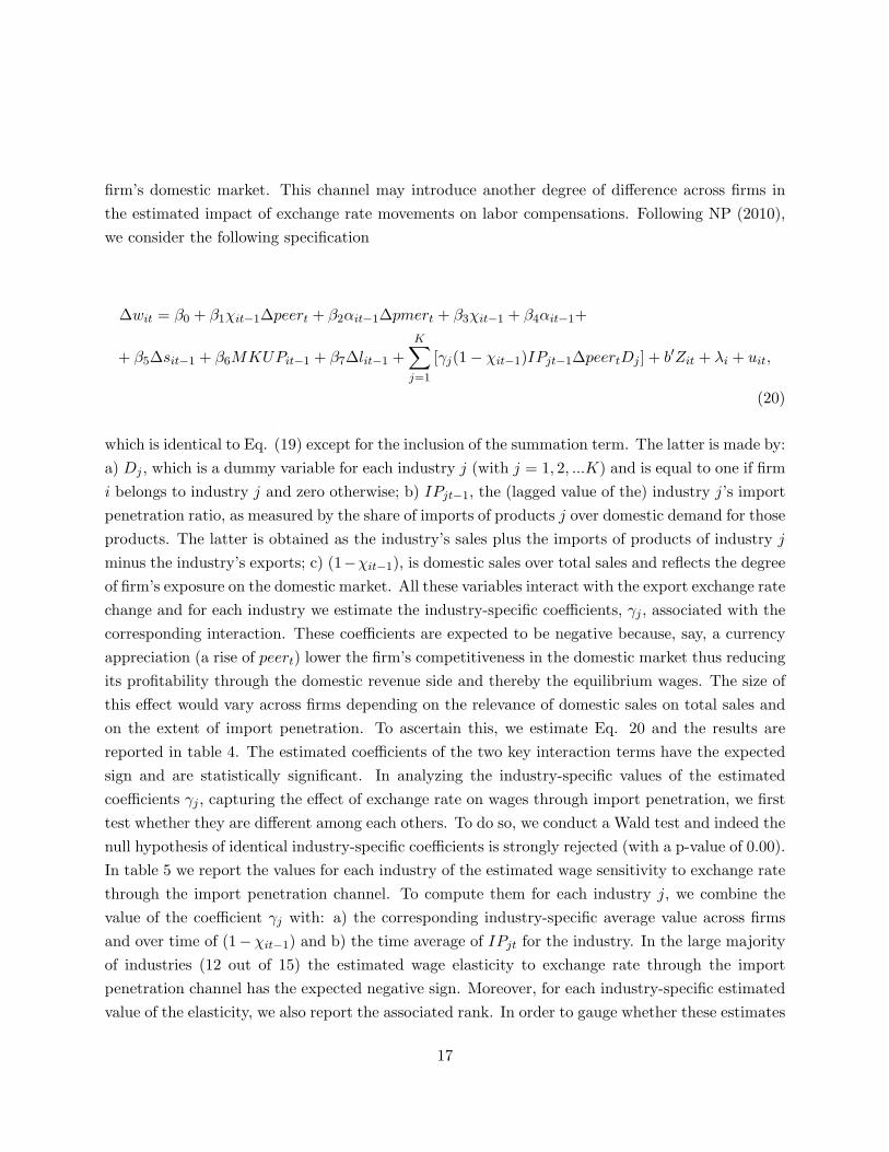
firm’s domestic market. This channel may introduce another degree of difference across firms inthe estimated impact of exchange rate movements on labor compensations. Following NP (2010),we consider the following specification

∆wit = β0 + β1χit−1∆peert + β2αit−1∆pmert + β3χit−1 + β4αit−1+

+ β5∆sit−1 + β6MKUPit−1 + β7∆lit−1 +K∑j=1

[γj(1− χit−1)IPjt−1∆peertDj ] + b′Zit + λi + uit,

(20)

which is identical to Eq. (19) except for the inclusion of the summation term. The latter is made by:a) Dj , which is a dummy variable for each industry j (with j = 1, 2, ...K) and is equal to one if firmi belongs to industry j and zero otherwise; b) IPjt−1, the (lagged value of the) industry j’s importpenetration ratio, as measured by the share of imports of products j over domestic demand for thoseproducts. The latter is obtained as the industry’s sales plus the imports of products of industry jminus the industry’s exports; c) (1−χit−1), is domestic sales over total sales and reflects the degreeof firm’s exposure on the domestic market. All these variables interact with the export exchange ratechange and for each industry we estimate the industry-specific coefficients, γj , associated with thecorresponding interaction. These coefficients are expected to be negative because, say, a currencyappreciation (a rise of peert) lower the firm’s competitiveness in the domestic market thus reducingits profitability through the domestic revenue side and thereby the equilibrium wages. The size ofthis effect would vary across firms depending on the relevance of domestic sales on total sales andon the extent of import penetration. To ascertain this, we estimate Eq. 20 and the results arereported in table 4. The estimated coefficients of the two key interaction terms have the expectedsign and are statistically significant. In analyzing the industry-specific values of the estimatedcoefficients γj , capturing the effect of exchange rate on wages through import penetration, we firsttest whether they are different among each others. To do so, we conduct a Wald test and indeed thenull hypothesis of identical industry-specific coefficients is strongly rejected (with a p-value of 0.00).In table 5 we report the values for each industry of the estimated wage sensitivity to exchange ratethrough the import penetration channel. To compute them for each industry j, we combine thevalue of the coefficient γj with: a) the corresponding industry-specific average value across firmsand over time of (1−χit−1) and b) the time average of IPjt for the industry. In the large majorityof industries (12 out of 15) the estimated wage elasticity to exchange rate through the importpenetration channel has the expected negative sign. Moreover, for each industry-specific estimatedvalue of the elasticity, we also report the associated rank. In order to gauge whether these estimates

17

are sensible, in table 5 we compare these estimates of the elasticities with the corresponding valuesof import penetration for each industry reported in the table with the associated rank. As foundin NP (2010) for the employment elasticity, it turns out that the estimated impact of exchangerate on wages through the domestic sales side is larger for industries exhibiting a higher degree ofimport penetration. The strongest effects are recorded for Electrical Machinery and for Computersand Office equipments. For the latter industry, the extent of import penetration is very high (58per cent; ranked n. 1) and for Electrical Machinery it is also sizeable (29 per cent; ranked n. 4).We have also computed the Spearman’s rank correlation between a) the (absolute values of the)estimated industry-specific wage responses on the domestic sale side and b) the indexes of importpenetration of the corresponding industries. The value of the Spearman correlation is 0.65 andthe null hypothesis that these two variables are independent is rejected at the 1 per cent level ofstatistical significance.

Moreover, focusing on the effects through the cost side, we point to differences across firms inthe degree of substitutability between imported intermediate inputs and domestically producedinputs. For example, after a severe depreciation that increases the price of imported inputs inthe domestic currency, a firm may decide to replace its imports of intermediate goods with similargoods that are domestically produced. Arguably, the extent to which this happens is likely to reflecttechnological and organizational characteristics of the firm, that to some extent are shared by thefirms in the same industry. If the extent of this substitutability is relatively high (low), then thewage sensitivity to exchange rate through the cost side channel would be relatively low (high). Toinvestigate if the different degree of substitutability between types of intermediate inputs introducesa significant source of heterogeneity across industries in the wage responsiveness to exchange ratealong the expenditure side, we estimate an equation that is identical to Eq. (19), except for theeffect of αit−1∆pmert on wages being estimated separately for each industry. To do so, we use thedummy variables for each industry Dj , as a further multiplicative term of the αit−1∆pmert term.To ascertain if the differences between the estimated coefficients summarizing the cost-side effectsof exchange rate on wages are significant, we performed a Wald test for the null hypothesis thatthese differences are equal to zero. The value of the test is 68.7 with a p-value of 0.00, indicatingthat differences across industries in the wage sensitivity through the cost side are statisticallysignificant. To conserve space, we do not report the regression results but we emphasize that theeffect of exchange rate on wages through the revenue side continues to be statistically significant(the estimated coefficient of χit−1∆peert is -0.480 with a standard error of 0.239).

18

5.2 Share of Newly Hired Workers and Composition of the Labor Force

We also investigate other feature that may provide a source of heterogeneity across firms in thewage elasticity to exchange rate. A first aspect deals with the transition of a worker from one firmto another and in particular on whether the effect of exchange rate on a worker’s wage is affectedby being a job stayer or a job changer. Goldberg and Tracy (2003) point to three different channelsof transmission of an exchange rate shock to the worker’s wage. While the standard channel is theon-the-job wage adjustment in the aftermath of the shock, exchange rate may also influence: a)the likelihood of a job switch and b) the size of the revision of the worker’s wage conditional to ajob transition. Using micro-labor data on individual employees, they indeed document a significanteffect of exchange rate on the amount of the worker’s wage adjustment associated with a job switch.

Using our firm-level data, we focus on the hiring rate for each firm in a given year and investigatewhether firms that are similar in all dimensions (e.g. international exposure) except for the percent-age of newly hired employees in a given year do exhibit a different responsiveness of the (average)wage to an exchange rate shock. A large size of the hiring rate in a given year implies that thefirm has among its employees a large share of job changers who have switched job in that year. Toappraise the effect of it on the firm’s wage sensitivity to exchange rate, we consider an empiricalspecification which includes the time-varying firm’s hiring rate. Specifically, we augment the twointeraction terms of the exchange rate variation with each of the firm’s international orientationindicators (respectively, χit−1 and αit−1) with the hiring rate, hirrit, also. The two key regressorstherefore become the following: 1) χit−1 ·∆peert · hirrit and 2) αit−1 ·∆pmert · hirrit. Of course,the term hirrit also enters in isolation in the specification, exactly as χit−1 and αit−1 do. Thehiring rate is computed as the share of newly hired workers in a given year over the total numberof employees (the latter is calculated as the simple average between firm’s employment in periods tand t−1). Table 6 documents that the wage sensitivity to exchange rate tends to increase with therate of firm’s hiring in a given year. Indeed, we estimate that the higher is hirrit the stronger is thewage responsiveness to the currency shock along both transmission channels related to the firm’sforeign exposure (the one though foreign sales and the one through imported intermediate inputs).For example, if we focus on labor compensation per employee, the estimated effect of exchange rateon the export side is negative and statistically significant (-3.875 with a standard error of 1.097)and the one on the imported input side is positive and significant (9.765 with a standard error of3.495). Although a thorough investigation of this issue would require data at both the firm and theindividual worker level, we argue that our finding on firm’s data complements the one uncoveredby Golberg and Tracy (2003) on individual workers data not controlling for firms’ characteristics.

19

Finally, we focus on the composition of the firm’s workforce by type of employees and ask ourselveswhether this affects the wage sensitivity to currency swings. We find that it does. In particular,although our data do not provide information on the characteristics of individual worker, we havehowever information for each firm and in each year on the composition of the firm’s workers bytype (blue-collar vis-a-vis white collars). Hence, similarly to CG (2001) and NP (2010) we estimatea simple panel specification in which the estimated firm-specific exchange rate elasticities of wagesis regressed on the firm’s share of blue-collar employees over total workers. The dependent variableis derived from the results of table 1 (column 1) as (2.608 · αit−1 − 0.722 · χit−1). The resultsare reported in table 7 and, perhaps not surprisingly, they indicate that a higher incidence in thefirm of the blue-collar employees (vis-a-vis the white-collars) is conducive to lower estimated wagesensitivity to exchange rate fluctuations.

6 Concluding Remarks

Using data on a representative panel of manufacturing firms we find that exchange rate fluctuationsdo affect the labor compensation set by each firm. Similarly to the analysis in NP (2010) on theresponse of employment conducted on the same microeconomic data, we find that the direction andsize of wage adjustment is determined by the external orientation of each firm on both the revenueand cost side of its balance sheet. Through the revenue side, a currency depreciation affects firm’sprofitability and thereby the equilibrium outcome of wages. The latter are shown to rise along thischannel and the effect is estimated to be larger the higher is the firm’s exposure to revenues fromexporting. On the other hand, a depreciation leads to a reduction of the firm’s wages through thechannel of expenditure for imported inputs and the effect is larger the higher is the firm’s reliance onimported inputs vis-a-vis domestically produced inputs. Our results indicate that, for a given typeof firm’s international exposure, the responsiveness of wages to exchange rate is more pronouncedfor firms with a lower degree of pricing power. Moreover, to provide further characterizations of thewage sensitivity, we also document that other transmission channels introduce a significant sourceof heterogeneity across firms in the response of wages to exchange rate swings. These include theextent of competition in the domestic marked exerted by foreign producers, as measured by theimport penetration in the domestic industry to which a firm belongs. Second, we consider the extentof substitutability in firm’s production between imported intermediate inputs and domesticallyproduced inputs. We also analyze the percentage of newly hired workers of a firm in a given yearand document that a larger presence in the firm of job changers affects the size of wage adjustmentin response to exchange rate variations. Finally, we find that the composition by type of the firm’s

20

labor force does influence the exchange rate elasticity of wages, with the latter being larger thehigher is the incidence in the firm of white-collar employees.

21

Figure 1

Real import and export exchange rates (1998 = 100)

90

95

100

105

110

115

120

125

Import

Export

80

85

90

95

100

105

110

115

120

125

Import

Export

Source: Bank of Italy.

22

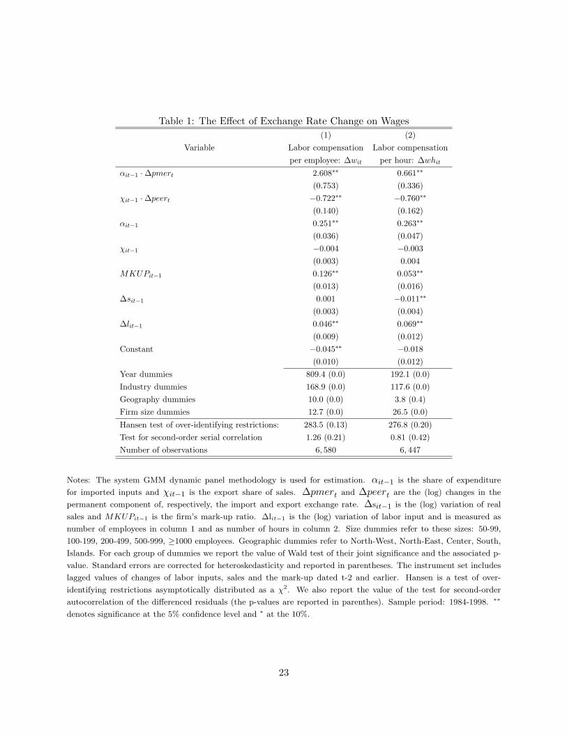
Table 1: The Effect of Exchange Rate Change on Wages(1) (2)

Variable Labor compensation Labor compensationper employee: ∆wit per hour: ∆whit

αit−1 ·∆pmert 2.608∗∗ 0.661∗∗

(0.753) (0.336)χit−1 ·∆peert −0.722∗∗ −0.760∗∗

(0.140) (0.162)αit−1 0.251∗∗ 0.263∗∗

(0.036) (0.047)χit−1 −0.004 −0.003

(0.003) 0.004MKUPit−1 0.126∗∗ 0.053∗∗

(0.013) (0.016)∆sit−1 0.001 −0.011∗∗

(0.003) (0.004)∆lit−1 0.046∗∗ 0.069∗∗

(0.009) (0.012)Constant −0.045∗∗ −0.018

(0.010) (0.012)Year dummies 809.4 (0.0) 192.1 (0.0)Industry dummies 168.9 (0.0) 117.6 (0.0)Geography dummies 10.0 (0.0) 3.8 (0.4)Firm size dummies 12.7 (0.0) 26.5 (0.0)

Hansen test of over-identifying restrictions: 283.5 (0.13) 276.8 (0.20)Test for second-order serial correlation 1.26 (0.21) 0.81 (0.42)Number of observations 6, 580 6, 447

Notes: The system GMM dynamic panel methodology is used for estimation. αit−1 is the share of expenditure

for imported inputs and χit−1 is the export share of sales. ∆pmert and ∆peert are the (log) changes in the

permanent component of, respectively, the import and export exchange rate. ∆sit−1 is the (log) variation of real

sales and MKUPit−1 is the firm’s mark-up ratio. ∆lit−1 is the (log) variation of labor input and is measured as

number of employees in column 1 and as number of hours in column 2. Size dummies refer to these sizes: 50-99,

100-199, 200-499, 500-999, ≥1000 employees. Geographic dummies refer to North-West, North-East, Center, South,

Islands. For each group of dummies we report the value of Wald test of their joint significance and the associated p-

value. Standard errors are corrected for heteroskedasticity and reported in parentheses. The instrument set includes

lagged values of changes of labor inputs, sales and the mark-up dated t-2 and earlier. Hansen is a test of over-

identifying restrictions asymptotically distributed as a χ2. We also report the value of the test for second-order

autocorrelation of the differenced residuals (the p-values are reported in parenthes). Sample period: 1984-1998. ∗∗

denotes significance at the 5% confidence level and ∗ at the 10%.

23

Table 2: Exchange rate, Market Power and Wage Adjustment (I)

(1) (2) (3) (4)

Variable Compensation per employee: ∆wit Compensation per hour: ∆whit

Degree of market power Degree of market powerLow High Low High

αit−1 ·∆pmert 2.848∗∗ 2.743∗∗ 3.751∗∗ 0.528∗∗

(0.819) (0.891) (1.204) (0.318)

χit−1 ·∆peert −1.281∗∗ −0.375∗∗ −1.182∗∗ −0.302∗∗

(0.163) (0.170) (0.229) (0.137)

αit−1 0.368∗∗ 0.215∗∗ 0.366∗∗ 0.285∗∗

(0.055) (0.049) (0.068) (0.048)

χit−1 −0.007 −0.001 −0.007 0.001

(0.005) (0.004) (0.006) (0.005)

∆sit−1 0.016∗∗ −0.016∗∗ −0.006∗∗ −0.018∗∗

(0.003) (0.004) (0.003) (0.003)

MKUPit−1 0.127∗∗ 0.168∗∗ 0.114∗∗ 0.194∗∗

(0.012) (0.034) (0.015) (0.027)

∆lit−1 0.083∗∗ −0.015 0.147∗∗ 0.072

(0.010) (0.014) (0.009) (0.009)

Constant −0.053∗∗ −0.051∗∗ −0.006 −0.058∗∗

(0.013) (0.015) (0.019) (0.015)

Year dummies 430.2 (0.0) 489.3 (0.0) 121.0 (0.0) 210.3 (0.0)

Industry dummies 76.2 (0.0) 85.1 (0.0) 36.5 (0.0) 137.3 (0.0)

Geography dummies 14.0 (0.0) 15.7 (0.0) 15.2 (0.0) 18.9 (0.0)

Firm size dummies 6.8 (0.2) 10.0 (0.0) 12.5 (0.0) 24.4 (0.0)

Hansen test ofover-identifying restrictions 260.9 (0.16) 210.5 (0.09) 248.8 (0.17) 275.5 (0.22)

Test for second-orderserial correlation 1.18 (0.24) 1.82 (0.07) 0.60 (0.55) −0.54 (0.59)

Number of observations 3, 335 3, 245 3, 123 3, 212

Notes: see Table 1. The system GMM dynamic panel methodology is used for estimation. The sample is split based

on the degree of firms’market power. The threshold criterion is the median of firms’mark-up. Variables in lower-case

letters denote their logarithmic transformation. ∗∗ denotes significance at the 5% confidence level and ∗ at the 10%

level.

24

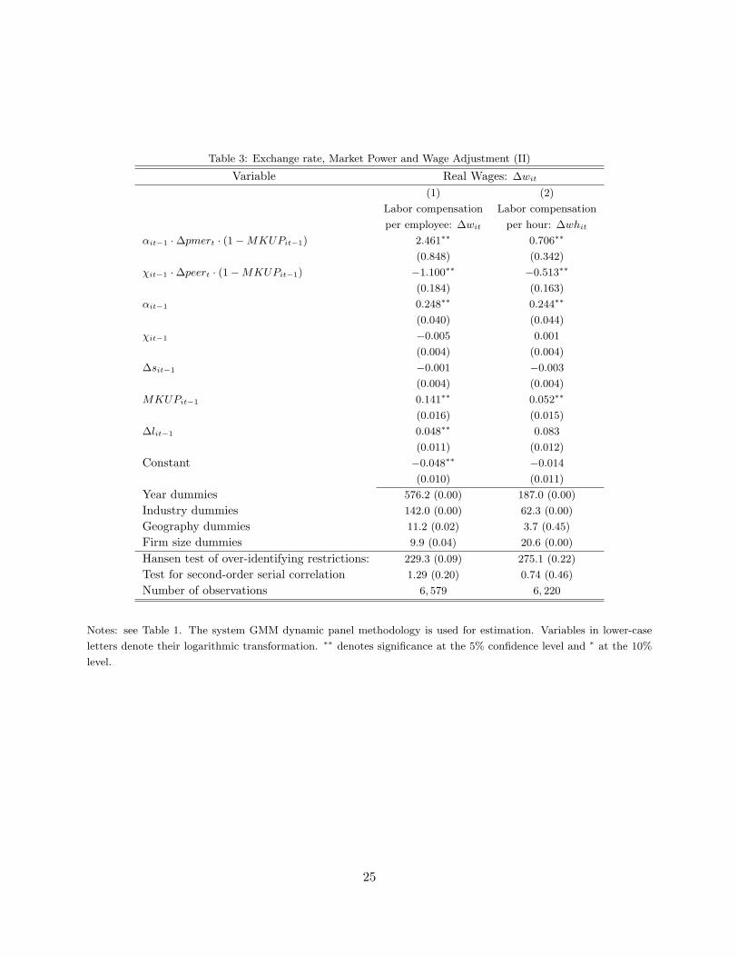
Table 3: Exchange rate, Market Power and Wage Adjustment (II)

Variable Real Wages: ∆wit

(1) (2)

Labor compensation Labor compensation

per employee: ∆wit per hour: ∆whit

αit−1 ·∆pmert · (1−MKUPit−1) 2.461∗∗ 0.706∗∗

(0.848) (0.342)

χit−1 ·∆peert · (1−MKUPit−1) −1.100∗∗ −0.513∗∗

(0.184) (0.163)

αit−1 0.248∗∗ 0.244∗∗

(0.040) (0.044)

χit−1 −0.005 0.001

(0.004) (0.004)

∆sit−1 −0.001 −0.003

(0.004) (0.004)

MKUPit−1 0.141∗∗ 0.052∗∗

(0.016) (0.015)

∆lit−1 0.048∗∗ 0.083

(0.011) (0.012)

Constant −0.048∗∗ −0.014

(0.010) (0.011)

Year dummies 576.2 (0.00) 187.0 (0.00)

Industry dummies 142.0 (0.00) 62.3 (0.00)

Geography dummies 11.2 (0.02) 3.7 (0.45)

Firm size dummies 9.9 (0.04) 20.6 (0.00)

Hansen test of over-identifying restrictions: 229.3 (0.09) 275.1 (0.22)

Test for second-order serial correlation 1.29 (0.20) 0.74 (0.46)

Number of observations 6, 579 6, 220

Notes: see Table 1. The system GMM dynamic panel methodology is used for estimation. Variables in lower-case

letters denote their logarithmic transformation. ∗∗ denotes significance at the 5% confidence level and ∗ at the 10%

level.

25

Table 4: Exchange Rate, Import Penetration and Wage Adjustment

Variable Labor compensationper employee: ∆wit

αit−1 ·∆pmert 5.809∗∗

(2.482)

χit−1 ·∆peert −2.130∗∗

(1.0841)

(1− χit−1) ·∆peert · IP1t−1 ·D1, (1− χit−1) ·∆peert · IP2t−1 ·D2,.... Wald test:

...,(1− χit−1) ·∆peert · IPKt−1 ·DK 40.3 (p-val: 0.00)

αit−1 0.120∗

(0.063)

χit−1 −0.009∗

(0.005)

∆sit−1 −0.001

(0.004)

MKUPit−1 0.033∗∗

(0.014)

∆lit−1 −0.017

(0.016)

Constant −0.009

(0.031)

Year dummies 219.0 (0.00)

Industry dummies 52.8 (0.00)

Geography dummies 11.9 (0.02)

Firm size dummies 5.2 (0.27)

Hansen test of over-identifying restrictions: 175.2 (0.40)

Test for second-order serial correlation 1.50 (0.13)

Number of observations 5, 183

Notes: see Table 1. The system GMM dynamic panel methodology is used for estimation. IPjt is the value of import

penetration experienced by industry j (to which firm i belongs) in the year t. Dj is the j-th industry dummy, taking

the value of one if firm i belongs to industry j and zero otherwise. The Wald statistic associated with the variables

(1−χit−1) ·∆peert · IPjt−1 ·Dj (j=1,2,..., K ) tests for the joint hypothesis that their coefficients are equal. Variables

in lower-case letters denote their logarithmic transformation. ∗∗ denotes significance at the 5% confidence level and∗ at the 10% level.

26

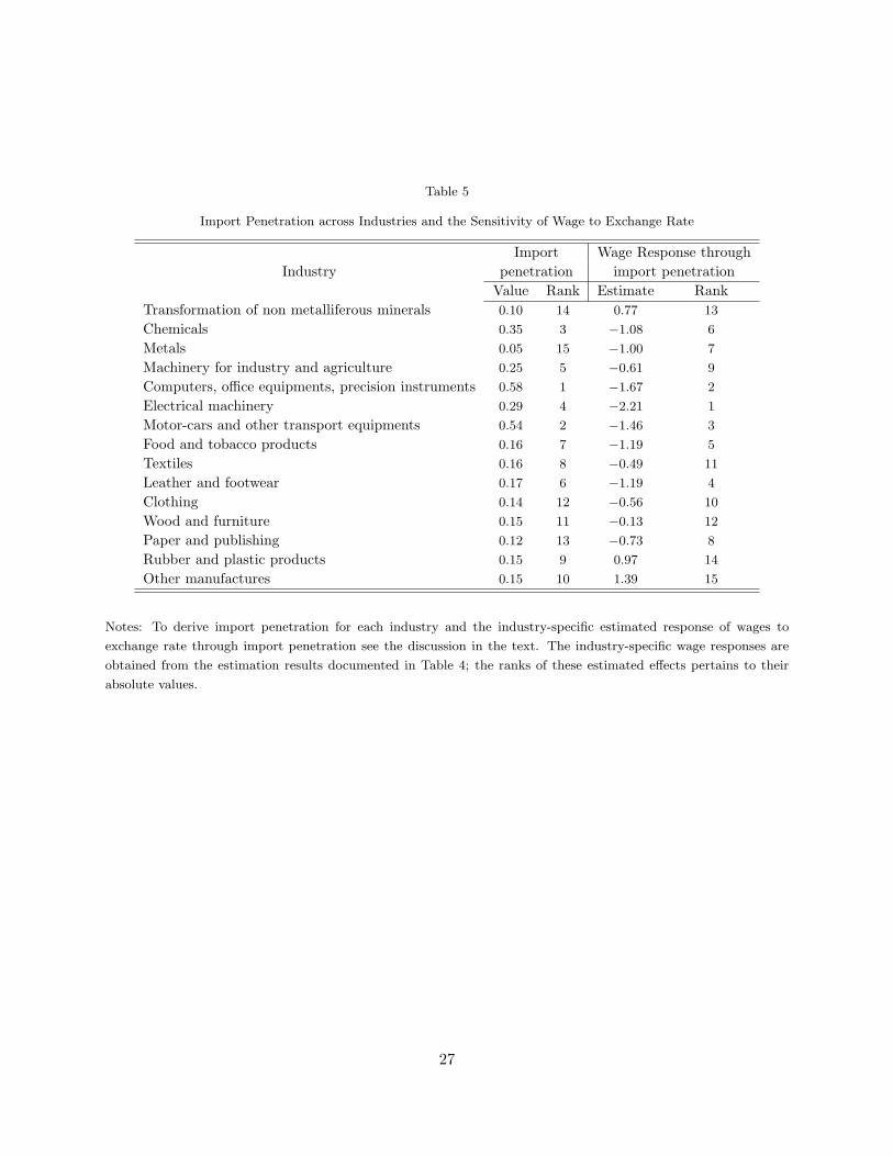
Table 5

Import Penetration across Industries and the Sensitivity of Wage to Exchange Rate

Import Wage Response throughIndustry penetration import penetration

Value Rank Estimate RankTransformation of non metalliferous minerals 0.10 14 0.77 13

Chemicals 0.35 3 −1.08 6

Metals 0.05 15 −1.00 7

Machinery for industry and agriculture 0.25 5 −0.61 9

Computers, office equipments, precision instruments 0.58 1 −1.67 2

Electrical machinery 0.29 4 −2.21 1

Motor-cars and other transport equipments 0.54 2 −1.46 3

Food and tobacco products 0.16 7 −1.19 5

Textiles 0.16 8 −0.49 11

Leather and footwear 0.17 6 −1.19 4

Clothing 0.14 12 −0.56 10

Wood and furniture 0.15 11 −0.13 12

Paper and publishing 0.12 13 −0.73 8

Rubber and plastic products 0.15 9 0.97 14

Other manufactures 0.15 10 1.39 15

Notes: To derive import penetration for each industry and the industry-specific estimated response of wages to

exchange rate through import penetration see the discussion in the text. The industry-specific wage responses are

obtained from the estimation results documented in Table 4; the ranks of these estimated effects pertains to their

absolute values.

27

Table 6

Exchange rate, Newly Hired Workers and Wage Adjustment

Variable Real Wages: ∆wit

(1) (2)

Labor compensation Labor compensation

per employee: ∆wit per hour: ∆whit

αit−1 ·∆pmert · hirrit 9.765∗∗ 8.246∗∗

(3.495) (3.416)

χit−1 ·∆peert · hirrit −3.875∗∗ −4.508∗∗

(1.097) (1.391)

hirrit −0.007 −0.020

(0.007) (0.007)

αit−1 0.254∗∗ 0.247∗∗

(0.037) (0.047)

χit−1 −0.002 −0.001

(0.003) (0.004)

∆sit−1 0.001 −0.008∗∗

(0.003) (0.004)

mkupit−1 0.121∗∗ 0.051∗∗

(0.013) (0.016)

∆lit−1 0.043∗∗ 0.065∗∗

(0.001) (0.013)

Constant −0.045∗∗ −0.010

(0.010) (0.012)

Year dummies 807.2 (0.00) 195.2 (0.00)

Industry dummies 190.7 (0.00) 116.9 (0.00)

Geography dummies 7.1 (0.13) 3.5 (0.47)

Firm size dummies 9.7 (0.05) 25.0 (0.00)

Hansen test of over-identifying restrictions: 279.9 (0.17) 275.6 (0.22)

Test for second-order serial correlation 1.20 (0.23) 0.82 (0.41)

Number of observations 6, 580 6, 447

Notes: see Table 1. The system GMM dynamic panel methodology is used for estimation. Variables in lower-case

letters denote their logarithmic transformation. hirrit is the hiring rate as defined in the text. ∗∗ denotes significance

at the 5% confidence level and ∗ at the 10% level.

28

Table 7

Workers Type and the Response of Wage to Exchange Rate

Dependent variable:Estimated Wage Response (see table 1)

2.608 · αit−1 − 0.722 · χit−1

VariableNum Blue Collarsit

Num Totalit−0.062∗∗

(0.014)

Constant −0.061

(0.061)

Year dummies 129.0 (0.00)

Industry dummies 9.5 (0.00)

Geography dummies 0.3 (0.86)

Firm size dummies 6.4 (0.00)

Hausman test 288.4 (0.00)

Number of observations 9, 950

Notes: The dependent variable is the estimated response of compensation per employee to permanent exchange

rate variations as obtained by estimating the equation whose results are documented in Table 1 (column 1). The

explanatory variable is the firm-level share of blue-collar workers over total workers. The fixed effects panel estimation

method has been applied and values of the Hausman test are reported (with the associated p-value). ∗∗ denotes

significance at the 5% confidence level and ∗ at the 10% level.

29

References

[1] Arellano, M. and S. R. Bond (1991), “Some Tests of Specification for Panel Data: Monte Carlo Evidence and

an Application to Employment Equations”, Review of Economic Studies, 58, 277-297.

[2] Arellano, M. and O. Bover (1995), “Another Look at the Instrumental Variable Estimation of Error-components

Models”, Journal of Econometrics, 68, 29-51.

[3] Banca d’Italia (1998), “Nuovi Indicatori di Tasso di Cambio Effettivo Nominale e Reale”, Bollettino Economico

30, 1*-8*.

[4] Bernard, A.B., J.B. Jensen, S.J. Redding and P.K. Schott (2007), “Firms In International Trade”, Journal of

Economic Perspectives, 21, 105-130.

[5] Beveridge, S. and C. R. Nelson (1981), “New Approach to Decomposition of Economic Time Series into Perma-

nent and Transitory Components with Particular Attention to Measurement of the ’Business Cycle’, Journal of

Monetary Economics, 7, 151-174.

[6] Blundell, R. and S. Bond (2000), “GMM Estimation with Persistent Panel Data: an Application to Production

Functions”, Econometric Reviews, 19, 321-340.

[7] Campa, J. and L. Goldberg, (1999), “Investment, Pass-Through and Exchange Rates: a Cross-Country Com-

parison”, International Economic Review, 40, 287-314.

[8] Campa, J. and Goldberg, L. (2001), “Employment versus Wage Adjustment and the U.S. Dollar”, Review of

Economics and Statistics, 83, 477-489.

[9] Domowitz, I., R. G. Hubbard and C. Petersen, (1986), “Business Cycles and the Relationship between Concen-

tration and Profit Margins”, Rand Journal of Economics 17, 1-17.

[10] Dornbusch, R. (1987), “Exchange Rates and Prices”, American Economic Review, 77, 93-106.

[11] Goldberg, L. and J. Tracy (2000), “Exchange Rates and Local Labor Markets”, in R. Feenstra (ed.), The Impact

of International Trade on Wages, NBER and University of Chicago Press.

[12] Goldberg, L. and J. Tracy (2003), “Exchange Rates and Wages”, Revided version of the NBER working paper

n. 8137, 2001.

[13] Kletzer, L . (2000), “Trade and Job Loss in U.S. Manufacturing, 1979-94”, in R. Feenstra (ed.), The Impact of

International Trade on Wages, NBER and University of Chicago Press.

[14] Knetter, M. (1993), “International Comparisons of Pricing-to Market Behavior”, American Economic Review,

83, 473-486.

[15] Nucci, F. and A.F. Pozzolo (2001), “Investment and the Exchange Rate: an Analysis with Firm-Level Panel

Data”, European Economic Review, 45, 259-283.

[16] Nucci, F. and A.F. Pozzolo (2010), Exchange rate, Employment and Hours: what Firm-level Data Say, (2010),

Journal of International Economics, 82, 112123.

[17] Revenga, A. (1992), “Exporting Jobs? The Impact of Import Competition on mployment and Wages in U.S.

Manufacturing”, Quarterly Journal of Economics, 94, S111-143.

[18] Yang, J., (1997), “Exchange Rate Pass-through in U.S. Manufacturing Industries”, Review of Economics and

Statistics, 79, 95-104.

30