
Excess Capacity and Effectiveness of Policy Interventions ... · DP RIETI Discussion ... using...
31
DP RIETI Discussion Paper Series 18-E-012 Excess Capacity and Effectiveness of Policy Interventions: Evidence from the cement industry OKAZAKI Tetsuji RIETI ONISHI Ken Singapore Management University WAKAMORI Naoki University of Tokyo The Research Institute of Economy, Trade and Industry http://www.rieti.go.jp/en/
Transcript of Excess Capacity and Effectiveness of Policy Interventions ... · DP RIETI Discussion ... using...

DPRIETI Discussion Paper Series 18-E-012
Excess Capacity and Effectiveness of Policy Interventions: Evidence from the cement industry
OKAZAKI TetsujiRIETI
ONISHI KenSingapore Management University
WAKAMORI NaokiUniversity of Tokyo
The Research Institute of Economy, Trade and Industryhttp://www.rieti.go.jp/en/

RIETI Discussion Paper Series 18-E-012
March 2018
Excess Capacity and Effectiveness of Policy Interventions: Evidence from the cement industry*
OKAZAKI Tetsuji† ONISHI Ken‡ WAKAMORI Naoki§
Abstract
Excess production capacity has been a major concern in many countries, in particular, when an industry faces declining demand. Strategic interaction among firms might delay efficient scrappages of production capacity, and policy interventions that eliminate such strategic incentives may improve efficiency. This paper empirically studies the effectiveness of policy interventions in such environment, using plant-level data on the Japanese cement industry. Our estimation results show that a capacity coordination policy that forces firms to reduce their excessive production capacity simultaneously can effectively reduce excess capacity without distorting firms' scrappage decisions or increasing the market power of the firms.
Keywords: Excess capacity, Capacity coordination, Cement, Industrial policy
JEL classification: D24, L13, L52, L61.
RIETI Discussion Papers Series aims at widely disseminating research results in the form of professional
papers, thereby stimulating lively discussion. The views expressed in the papers are solely those of the
author(s), and neither represent those of the organization to which the author(s) belong(s) nor the Research
Institute of Economy, Trade and Industry.
*This work has been supported by JSPS KAKENHI Grant Number JP26285053. It is also financially supported byCanon Institute for Global Studies (CIGS). This study is conducted as a part of the project “Historical evaluation ofindustrial policy” undertaken at the Research Institute of Economy, Trade and Industry (RIETI). The authors aregrateful for helpful comments and suggestions by Naoshi Doi, Mitsuru Igami, Masayuki Morikawa, MasatoNishiwaki and Makoto Yano. We also wish to thank the participants at many conferences and seminars, includingDiscussion Paper seminar participants at RIETI. We also wish to thank Japan Cement Association for providinghistorical documents on the capacity coordination policy in the cement industry.† University of Tokyo, [email protected].‡ Singapore Management University, [email protected].§ (Corresponding Author) University of Tokyo, [email protected].

1 Introduction
Excess production capacity has been a major concern in many countries, in particular,
when an industry faces declining demand, e.g., the US steel industry in the 1970s, the
shipbuilding industry in China and Korea, and the hard disk drive industry in Asia in the
2010s. The excess capacity literature dates back to at least Bain (1962), who defines excess
capacity as a “persistent tendency toward redundant capacity at times of maximum or peak
demand.” Excess production capacity is one source of social inefficiencies; it might cause
capital misallocation or limit land use. Policymakers have been particularly concerned about
this excess capacity issue, which has been a major topic in several high-level OECD meetings
since the 1970s and, more recently, in an OECD policy roundtable in 2011 that discussed
this problem of excess capacity in the context of competition law and policy. Although
policymakers have extensively discussed the best way to solve the issue of excess capacity,
economists have yet to provide a rigorous empirical economic analysis.
As shown theoretically by Ghemawat and Nalebuff (1990), the problem with excess capac-
ity may be resolved through natural selection; excess capacity may put downward pressure
on profits, resulting in divestment of unused production capacity and exit of firms from the
market. However, it is also well known that, in oligopolistic markets, firms’ strategic inter-
action may delay the process. Firms may keep their excess capacity if they can discourage
other firms’ production or if they are in a situation of “war of attrition” (Smith, 1974). If
such strategic considerations delay the process of capacity adjustment, public policies that
eliminate strategic incentives may help restore efficiency.
This paper studies a series of unique policy interventions introduced by the Japanese
government to solve the excess capacity problem in the cement industry in the 1980s and
1990s. Although the Japanese cement industry experienced strong growth in demand after
the World War II, the industry faced declining demand in the 1970s, triggered by two oil
crises. The oligopolistic firms in the industry did not divest their production capacity and
the Ministry of Industry and International Trade (hereinafter MITI) initiated a series of poli-
cies called “capacity coordination” that forced the cement firms to divest their production
capacity simultaneously, based on the allotment authorized by MITI. The first capacity co-
ordination policy, implemented between January 1985 and March 1986, targeted a reduction
of 30 million tons out of the 129 million tons of existing capacity. Out of the 30 million tons,
25 million tons was nonoperating capacity and five million tons was operating capacity. The
second capacity coordination policy, implemented between December 1988 and March 1991,
1

targeted a further reduction of 10.7 million tons of the existing 98 million tons, all of which
was operating capacity.
In our empirical analysis, we first show qualitatively that, even with declining demand,
the cement firms did not engage in divestment, which leads to the question of why these firms
retained their excess capacity. Our empirical analysis shows that their behavior was driven
by strategic interaction rather than their production needs. Here, strategic interaction does
not mean the firms retained their excess capacity to discourage other firms’ production, but
instead that the firms played an attrition game, expecting other firms to divest.
This paper then proceeds to evaluate the capacity coordination policy; in particular,
whether this policy intervention: (1) distorted the scrappage decisions of the firms, and (2)
increased their prices and/or markups. As for the first point, our estimation results show that
the firms were likely to divest inefficient plants before policy introduction and their scrappage
decision rules were unchanged during the policy implementation period. This result enables
us to conclude that capacity coordination could effectively reduce excess capacity without
distorting firms’ scrappage decisions. As for the second point, we first obtain the plant-
level marginal costs based on the first-order conditions for the firms and, using regression
analysis, find that both capacity coordination policies did not increase markups charged by
the cement firms.
These results might be counterintuitive, as capacity coordination policies are typically
viewed as an anticompetitive policy intervention. In particular, after the second policy in-
tervention when the cement firms divested operating plants, we naturally expect that the
firms would have enhanced their market power. However, this was not the case and further
investigation finds that the cement firms concentrated their production within the remaining
plants and the utilization rates for those plants increased to almost 100%. In other words, al-
though the second capacity coordination policy forced the firms to shut down some operating
plants, they could meet demand with their remaining capacity. Thus, in some sense, these
divested plants were excess capacity. Of course, our estimation results for the first capacity
coordination policy suggest that, if a capacity coordination policy eliminates just excessive
capacity, then the policy would not lower consumer welfare. Therefore, if allotments and
total reduction capacity are well crafted, capacity coordination policy potentially accelerates
the divestment process without distorting firms’ scrappage decisions or lowering consumer
welfare.
This paper contributes to the literature on (1) declining industries, and (2) capacity
coordination. Even though the study of declining industries is becoming increasingly im-
2

portant, there is only a handful of theoretical and empirical studies in this area. Ghemawat
and Nalebuff (1985, 1990), Fudenberg and Tirole (1986), and Whinston (1988) consider an
oligopolistic market and examine the firms’ decisions to divest and/or exit when the in-
dustry faces declining demand. On the empirical side, Lieberman (1990), Deily (1991), and
Nishiwaki and Kwon (2013) study firms’ exit or plants’ closure behavior relating to the firms’
observable characteristics and unobserved productivity. More recently, Nishiwaki (2016) and
Takahashi (2015), using a structural approach, study firms’ exit and divestment decisions,
respectively, in declining industries. Nishiwaki (2016) examines the effect of mergers on
divestment behavior in the Japanese cement industry and finds that strategic interaction,
through business stealing in particular, distorts incentives for divestment. Takahashi (2015)
estimates an exit game played by US movie theaters, which builds upon a theoretical frame-
work developed by Fudenberg and Tirole (1986), and finds that strategic interaction among
the theaters delay the exit date substantially. Both results suggest that policy intervention
may help restore efficiency by eliminating strategic interaction among firms.
Excess capacity in declining industries creates social inefficiency, and one of the policy
instruments discussed among policymakers that can address this is capacity coordination.
Kamita (2010) investigates a recent case from the US airline industry: the Aloha–Hawaiian
immunity agreement. In response to declining demand after September 11, 2001, the US
Department of Transportation (DOT) allowed Aloha Airlines and Hawaiian Airlines to co-
ordinate capacity for a limited period of time.1 She finds that the two firms maintained high
prices not only during the immunity period, but also during the subsequent 2.5 years, until
a new competitor entered the market. Although empirical analysis on capacity coordination
is scarce, Hampton and Sherstyuk (2012) conducts an experimental study. They show that
capacity coordination by an enforceable institution, e.g., the government initiative in our
context or agreements with enforceable punishment in the Aloha–Hawaiian case, accelerates
the capital adjustment process. While their main focus is the effects of capacity coordination
on the prices and speed of the capital adjustment process, we also examine their implications
for effectiveness and efficiency of the capacity coordination policy.
This paper is organized as follows. Section 2 describes the industry and provides the
historical background of the Japanese cement industry, as well as the data used in our
empirical analysis. Our empirical models and estimation results are presented in Section 3.
Given our findings, we discuss the policy implications and caveats in Section 4. Section 5
concludes.
1See Blair, Mak and Bonham (2007) for more detailed information.
3
2 Industry and Historical Background
2.1 Cement
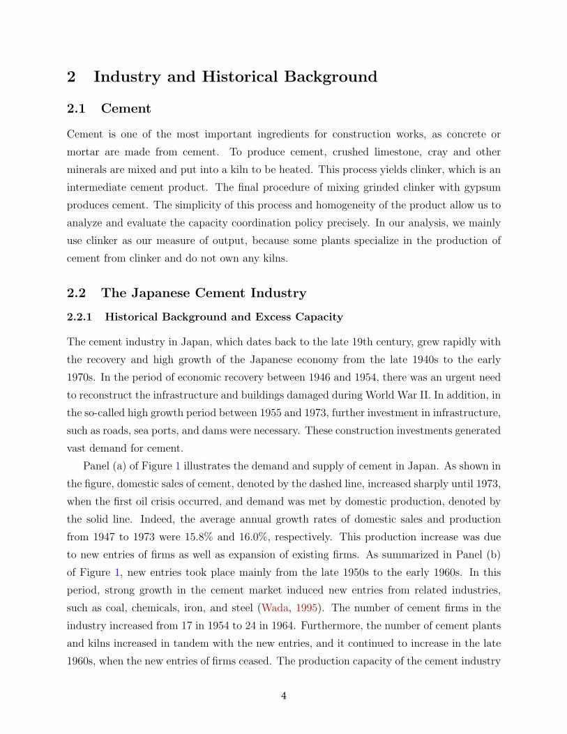
Cement is one of the most important ingredients for construction works, as concrete or
mortar are made from cement. To produce cement, crushed limestone, cray and other
minerals are mixed and put into a kiln to be heated. This process yields clinker, which is an
intermediate cement product. The final procedure of mixing grinded clinker with gypsum
produces cement. The simplicity of this process and homogeneity of the product allow us to
analyze and evaluate the capacity coordination policy precisely. In our analysis, we mainly
use clinker as our measure of output, because some plants specialize in the production of
cement from clinker and do not own any kilns.
2.2 The Japanese Cement Industry
2.2.1 Historical Background and Excess Capacity
The cement industry in Japan, which dates back to the late 19th century, grew rapidly with
the recovery and high growth of the Japanese economy from the late 1940s to the early
1970s. In the period of economic recovery between 1946 and 1954, there was an urgent need
to reconstruct the infrastructure and buildings damaged during World War II. In addition, in
the so-called high growth period between 1955 and 1973, further investment in infrastructure,
such as roads, sea ports, and dams were necessary. These construction investments generated
vast demand for cement.
Panel (a) of Figure 1 illustrates the demand and supply of cement in Japan. As shown in
the figure, domestic sales of cement, denoted by the dashed line, increased sharply until 1973,
when the first oil crisis occurred, and demand was met by domestic production, denoted by
the solid line. Indeed, the average annual growth rates of domestic sales and production
from 1947 to 1973 were 15.8% and 16.0%, respectively. This production increase was due
to new entries of firms as well as expansion of existing firms. As summarized in Panel (b)
of Figure 1, new entries took place mainly from the late 1950s to the early 1960s. In this
period, strong growth in the cement market induced new entries from related industries,
such as coal, chemicals, iron, and steel (Wada, 1995). The number of cement firms in the
industry increased from 17 in 1954 to 24 in 1964. Furthermore, the number of cement plants
and kilns increased in tandem with the new entries, and it continued to increase in the late
1960s, when the new entries of firms ceased. The production capacity of the cement industry
4

Figure 1: Industry Evolution over Time
Source: Japan Cement Association (1998), p.117.
increased even more rapidly in the 1950s and 1960s, as denoted by the solid line in Figure 2.
The first oil crisis in 1973 was a turning point of the postwar Japanese economy. In 1974,
the growth rate of real GDP became negative for the first time in the postwar period, and
put an end to the high growth of previous decades. In the 1950s and 1960s, the Japanese
economy continued to grow at around 10% per year, but after the first oil crisis the growth
rate fell to 4–5%. This slowdown in economic growth caused a decline in construction
investment. Moreover, the increase in the cumulative government deficit and the effort
toward fiscal reconstruction reduced public construction investment. The substantial decline
in construction investment after the first oil crisis caused a decline in domestic demand for
cement, as shown in panel (a) of Figure 1. In addition, the second oil crisis occurred in
1979. After the oil crises, excess capacity emerged in the cement industry. While demand
for cement declined, production capacity was maintained or increased slightly until 1985.
In the high growth period, the utilization rate of the equipment (production/capacity) was
5

Figure 2: Capacity and Utilization Rate
Source: Japan Cement Association (1998), p.118-119.
around 70–80%, although it fell below 70% during recessions. After the first oil crisis, the
utilization rate was consistently below 70% and sometimes fell below 60%, as in Figure 2.
2.2.2 Policy Interventions
The change in the economic environment after the two oil crises had a serious impact on the
cement industry. To maintain profitability under a sharp increase in the oil price, the cement
firms organized three series of “recession cartels” to reduce production. These cartels were
approved by the Japan Fair Trade Commission under the Antitrust Law. The terms of the
cartels were (1) November 11, 1975 to January 31, 1976, (2) June 24, 1977 to December 31,
1977, and (3) August 3, 1983 to December 31, 1983 (Japan Cement Association, ed, 1998:
pp.49–50). Although these recession cartels raised the cement price temporarily, they did
not promote divestment of capacity, which led to further policy intervention by MITI.
In 1984, the cement industry was subject to the Temporary Law for Structural Improve-
ment of the Special Industries (Tokutei Sangyo Kozo Kaizen Rinji Sochi Ho) with 25 other
industries, including electric furnace steelmaking, aluminum refining, and synthetic fiber
(Editorial Committee of the History of Trade and Industrial Policy and Okazaki, eds, 2012:
pp.52–3).2 This law aimed to reduce excess capacity in industries whose utilization rates of
2Prior to this law, a similar law called “the Temporary Law for Stabilization of the Special Recession
6

equipment remained low for a certain period of time, and MITI arranged capacity coordina-
tion in each designated industry by organizing cartels (“instructed cartels”). In August 1983,
the cement industry applied to MITI for a capacity coordination plan, which was approved
in April 1984, and the “Basic Plan for Structural Improvement of the Cement Industry” was
announced by MITI in August 1984 (Japan Cement Association, ed, 1998: p.51). To imple-
ment this capacity reduction plan, MITI instructed the cement firms to organize a cartel on
January 31, 1985 (Cement Press ed. 1985, p.18).
The plan consisted of two main components: (a) capacity coordination, and (b) orga-
nization of firms into five groups to promote cooperation within the groups. Regarding
capacity coordination, the plan prescribed that 30 million tons of the 129 million tons of
existing capacity for cement clinker be scrapped. Of this 30 million tons, 25 million tons
was nonoperating equipment and five million tons was operating equipment (Cement Press
ed. 1985, pp.16–7). Moreover, the allotment of capacity reduction to each firm was decided
through negotiation with the firms and MITI by January 1985. The allotment is shown in
Table 1 and indicates there was heterogeneity in divestment rates. The firms were required
to dispose of their excess capacity according to the allotment by the end of March 1985
except for six operating kilns, and these six operating kilns were to be disposed of by the
end of March 1986. To alleviate unequal allotment across the firms, monetary side-payments
were introduced.3 To smooth the implementation of capacity coordination, 23 cement firms
were organized into five groups, each of which established a new company for cooperative
businesses within the group, such as consignment production, joint sales, and arrangement
of transportation (Japan Cement Association, ed, 1998: p.51).4
By the end of March 1986, the divestment plan associated with the Temporary Law for
Structural Improvement of the Special Industries was completed. However, at that time,
the cement industry faced a new challenge, namely, a sharp appreciation of the yen after
the Plaza Agreement in September 1985. Because of the increase in imports and decline
in exports, excess capacity remained despite completion of the divestment plan. In the
meantime, because the Temporary Law for Structural Improvement of the Special Industries
was due to expire in June 1988, MITI prepared a new law for capacity reduction, the Law for
Facilitating Transformation of Industrial Structure (Sangyo Kozo Tenkan Enkatsuka Rinji
Industries” (Tokutei Fukyo Sangyo Antei Rinji Sochi Ho) was legislated in May 1978. Although the cementindustry was not subject to this earlier law, many other industries that were subject to the Temporary Lawfor Structural Improvement of the Special Industries were also subject to the earlier law.
3See Appendix A.4This grouping remained after the removal of the Temporary Law for Structural Improvement of the
Special Industries (Japan Cement Association, ed, 1998: p.53).
7

Table 1: Allotment of Capacity Reduction1st Policy Intervention 2nd Policy Intervention
Existing Reduction Existing ReductionGroup Firm capacity Amount % Capacity Amount %
1 Onoda Cement 15,378 5,605 36.4 9,840 746 7.6Mikawa Onoda Cement - - - 360 0 0.0Hitachi Cement 1,543 230 14.9 872 0 0.0Mitsui Kozan 3,827 1,618 42.3 2,209 0 0.0Shin-Nittetsu Kagaku 1,172 378 32.3 794 0 0.0Toyo Soda Kogyo 4,134 906 21.9 3,228 0 0.0
2 Nihon Cement 17,967 4,936 27.5 13,031 1,555 11.9Myojo Cement 3,150 699 22.2 2,451 0 0.0Daiichi Cement 1,449 357 24.6 1,092 0 0.0Osaka Cement 7,965 1,205 15.1 6,760 1,469 21.7
3 Mitsubishi Kogyo Cement 14,120 926 6.6 12,799 2,198 17.2Tokuyama Soda 6,886 1,780 25.8 5,106 0 0.0Tohoku Kaihatsu 0 0 2,314 0 0.0
4 Sumitomo Cement 12,558 1,833 14.6 10,112 1,677 16.6Hachinohe Cement 1,310 0 0 1,310 0 0.0Aso Cement 1,672 356 21.3 1,316 0 0.0Karita Cement 2,318 661 28.5 1,657 659 39.8Nittetsu Cement 1,789 282 15.8 1,507 0 0.0Denki Kagaku Kogyo 3,517 881 25 2,636 0 0.0
5 Ube Kosan 10,887 363 3.3 10,524 2,411 22.9Chichibu Cement 10,797 5,020 46.5 5,777 0 0.0Tsuruga Cement 1,893 248 13.1 1,645 0 0.0Ryukyu Cement 690 150 21.7 540 0 0.0
Total 125,615 29,027 23.1 97,880 10,705 10.9
Source: Cement Press (1989), p.47.Note: The values in the third, fourth, sixth and seventh columns are measured in thousands of tons.
Sochi Ho) in April 1987. Cement kilns were subject to this law, along with 22 other kinds of
equipment, and a capacity coordination policy similar to that under the Temporary Law for
Structural Improvement of the Special Industries was implemented (Editorial Committee of
the History of Trade and Industrial Policy and Okazaki, eds, 2012: pp.62-7). In December
1988, a divestment plan to scrap 10.7 million tons of the existing 98 million tons of capacity
was authorized by MITI, and this plan was completed by March 1991. At that time, however,
because of an increase in demand under the “Heisei bubble” boom, cement firms experienced
capacity shortages. Consequently, they applied to MITI to cancel their obligations under
the law, which was approved in May 1991 (Japan Cement Association, ed, 1998: pp.52-3).
2.3 Data Sources and Descriptive Statistics
We manually collect the data from various issues of Cement Yearbook (Cement Nenkan),
published by the Cement Press Co. Ltd. (Cement Shinbunsha), which is also used by Nishi-
8

Table 2: Summary StatisticsNum. of Obs. Mean Std. Dev. Min Max
Panel (a): Firm-Level Statistics# of Firms – – 20 24# of Plants within a Firm 2.50 1 1 11
Panel (b): Plant-Level StatisticsIn 1970 (beginning year)Monthly Capacity 54 128,815 80,133 25,000 350,000Production (clinker) 54 1,031,160 616,927 48,000 2,684,197Utilization 54 69.1% 20.7 9.3% 115.3%# of Workers 54 318.8 175.6 114 1205
In 1995 (last year)Monthly Capacity 40 202,656 123,469 55,167 588,417Production (clinker) 40 2,227,377 1,528,054 616,784 7,405,758Utilization 40 88.9% 10.8 54.4% 104.9%# of Workers 40 145.2 67.0 51 399
waki and Kwon (2013) and Nishiwaki (2016). This yearbook provides plant-level information
on monthly production capacity, production output (both clinkers and cement), number of
workers, number of kilns, size of individual kilns, kiln ownership, and the geographical lo-
cation of the plants. In terms of geographical location, we divide the territory of Japan
into eight areas, as in Nishiwaki (2016). We obtain the price of gypsum from the Corporate
Goods Price Index, published by the Bank of Japan. We use the price as an instrument
when estimating the demand function in our empirical analysis.
Summary statistics of our data, from 1970 to 1995, are given in Table 2. Panel (a)
presents two firm-level statistics: the number of firms and the number of plants within a
firm. The number of firms varies across the years in the sample, ranging from 20 to 24,
because of some entries and exits, as shown in Figure 1. The number of plants within a
firm varies substantially, ranging from 1 to 11, which indicates there is heterogeneity in firm
size. Panel (b) of Table 2 presents plant-level statistics for 1970 and 1995, the start and end
years of our sample. It is clear that the number of plants decreased from 54 to 40 during
this period. Both monthly capacity and annual production increased but the growth rate of
production was higher than that of monthly capacity, which resulted in a higher utilization
rate in 1995. Note that the average utilization rate in 1970 was about 70%, which is lower
than our expectation, as in 1970 the Japanese economy was still experiencing high growth
and it was prior to the first oil crisis. We can also see a dramatic decrease in the number of
workers: in 1970, the average number of workers was about 382, but in 1995 this had fallen
to 145. This change indicates that there was substantial technological advancement in the
form of automation and, as consequently, labor productivity increased sharply.
9

3 Empirical Analysis
Given our motivation stated in the previous section, this section attempts to evaluate the
policy introduced by the Japanese government. Before assessing the policy, however, we
first investigate why the firms have an incentive to keep their excess production capacity in
Subsection 3.1. Then, given our findings, we proceed to policy evaluation. In particular,
Subsection 3.2 examines whether or not the firms’ divestment decisions were distorted by
the policy, whereas Subsection 3.3 examines whether the policy affected the market power
of the cement firms.
3.1 Why did not the Firms Divest?
As shown in the previous section, the firms did not divest their production capacity even
though demand for cement was much lower than the industry’s total capacity. A natural
question then arises: “Why did the firms not divest their production facility?” In answering
this question, we first investigate the firms’ behavior theoretically to determine the pos-
sible impacts of holding (excess) capacity. Consider a dynamic oligopoly model, similar to
Nishiwaki (2016), with both static and dynamic decisions. Static decisions include choices re-
garding quantity, whereas dynamic decisions include investment/divestment and entry/exit.
This framework enables us to determine whether excess capacity could potentially affect
other firms through three distinct channels. Excess capacity may affect (1) quantity pro-
duced by rival firms, (2) investment or divestment of rival firms, and (3) entry or exit of
rival firms. The last channel is addressed in two different bodies of literature: strategic entry
deterrence as in Wenders (1971) and Spence (1977), and exit games as in Fudenberg and
Tirole (1986), Smith (1974), Ghemawat and Nalebuff (1985), and Takahashi (2015). In our
case, however, there were few entries or exits observed in the data, which does not allow us
to study such effects quantitatively. Therefore, in the following analysis, we focus on the
first and second channels which are closely related to each other.
The first channel examines the effect of investment, a dynamic decision, on the quantity
produced, a static decision. Naturally, firms cannot produce more than their capacity and
thus, quantity is affected by capacity choices as in Kreps and Scheinkman (1983). Moreover,
if production cost depends on production capacity (e.g., economies of scale), firms may
invest more to reduce their own production costs, which results in a change in production
quantities of their rivals. Even capacity has no direct impact on production costs; however,
unused capacity may still affect other firms’ production quantities in a repeated game. As
10

pointed out by Devidson and Deneckere (1990), by holding excess capacity, it is easier to
sustain collusion because excess capacity makes the punishment harsher. The second channel
has been studied mainly in growing industries since the seminal work of Spence (1979),
who unravel the preemptive role of investment. The literature has extended to declining
industries, both theoretically and empirically, as demonstrated by Ghemawat and Nalebuff
(1990) and Nishiwaki (2016). Motivated by these theoretical explanations of why firms
have an incentive to keep their production capacity, we empirically examine whether having
(excess) capacity affects the production and investment of other firms.
Impact of Excess Capacity on Quantity Produced We start by empirically investi-
gating the first channel, i.e., whether having (excess) capacity affects production. To do so,
consider the following static maximization problem of firm j:
maxqj
P (qj, q−j)qj − cj(qj) s.t. qj ≤ Kj,
where qj and q−j are the output of firm j and all other firms, respectively, cj(·) is a cost
function for firm j, and Kj is the maximum capacity that firm j can produce. When solving
for an equilibrium, the equilibrium quantity for firm j is expressed as:
q∗j = Q∗j(Kj, K−j),
which means that the equilibrium quantity is a function of capacities.5 Therefore, we first
estimate this relationship using the following specification:
[Specification 1] qj,t = α0 + α1Kj,t + α2
∑i=j
Ki,t + εj,t.
Here the parameter of interest is α2, which quantifies the impact of rivals’ capacity on
the quantity produced. Although Specification 1 is derived from a theoretical model and α2
reveals whether or not having capacity itself affects the production of other firms, we still
cannot determine whether having excess capacity affects production. To see the impact of
excess capacity on quantity produced, therefore, we further control for the total quantity
produced by other firms in Specification 2:
[Specification 2] qj,t = α0 + α1Kj,t + α2
∑i=j
Ki,t + α3
∑i=j
qi,t + εj,t.
5Note that cost differences across the firms are already captured by the differences in function Q∗j (·).
11

Intuitively, by adding the production quantity of the other firms, the coefficient on rivals’
capacity now captures the effect of excess capacity on own production. Furthermore, there is
one additional reason for controlling for the production quantity of the other firms. Produc-
tion technology in the cement industry might exhibit economies of scale, which implies that
a larger capacity may enable firms to produce cement at lower marginal cost. Suppose a rival
firm has a large production capacity. This cost advantage induces more output from this
rival firm and, in response to such a cost advantage, firm j must produce a smaller amount
because of strategic interaction. This effect arises from economies of scale, and Specification
1 cannot capture this effect separately from the other strategic effects of capacity. Thus,
we must control for production quantity of the other firms. If this is the only strategic role
of capacity, we would expect that α2 is zero. However, if capacity has some other strategic
roles, such as a threat of future punishment as found by Devidson and Deneckere (1990), we
would expect α2 to be negative.
Unfortunately, from an econometrics point of view, this relationship cannot be estimated
straightforwardly, as there is an endogeneity concern between qj,t and∑
i=j qi,t because of
simultaneity, and a possible nonlinearity concern with∑
i =j qi,t. Thus, we use an instrumen-
tal variable approach and flexibly control for∑
i=j qi,t. The instruments exploited here are
similar to that of Berry, Levinsohn and Pakes (1995), i.e., other firms’ quantity produced in
another area and other firms’ number of kilns in another area. Usage of this set of instru-
ments assumes that a firm having a cost advantage in one region must have the same cost
advantage in other regions. Hopefully, these instruments solve the endogeneity problem, but
to further ease concerns about endogeneity, we control for fixed effects for year, area, and
firm.
Impact of Excess Capacity on Investment Next, we empirically investigate the second
channel: whether the (excess) capacity of other firms affects investment. According to the
aforementioned literature, investment itself may have some strategic roles, i.e., investing in
capacity may deter investment by other firms. In our context, firms may delay divestment
because they expect divestment by other firms. Demonstrating such an effect, however,
is difficult because we cannot directly observe firms’ expectations. Rather, we employ the
following regression model to test our hypothesis:
[Specification 3] ij,t = α0 + α1
∑i=j
ii,t−1 + εj,t, where ij,t = Ki,t −Ki,t−1.
12

Table 3: Impact of Excess Capacity on ProductionSpecification 1 Specification 2 Specification 3
(i) OLS (ii) OLS (iii) IV (iv) IV (v) IV (vi) OLS (vii) OLS
Dependent Variable qj,t qj,t qj,t qj,t qj,t ij,t ij,t
Own Firm Capacity .950*** .948*** .955*** .955*** .961***
log(Kj) (.030) (.031) (.062) (.036) (.074)
Other Firm Capacity -.493*** -.502*** -.312 -.299 -.270
(log(∑
l =i Kl)) (.099) (.104) (.235) (.246) (.397)
Other Firm Quantity -.257 -.510 -14.99
log(∑
l =i ql) (.233) (1.814) (152.0)
Other Firm Quantity2 .008 -.934
(log(∑
l =i ql))2 (.056) (9.720)
Other Firm Quantity3 -.020
(log(∑
l =i ql))3 (.207)
Investment of Others -.120** -.101*∑i=j log(ii,t−1) (.055) (.054)
Own Investment -.142***
log(ij,t−1) (.041)
Other Controls√ √ √ √ √ √
Fixed Effects
Year√ √ √ √ √ √ √
Area√ √ √ √ √ √ √
Firm√ √ √ √ √ √ √
No. of Observations 461 461 419 419 419 388 388
Adjusted R2 .919 .919 .921 .920 .919 .083 .112
Note: Significance levels are denoted by < 0.10 (*), < 0.05 (**), and < 0.01 (***). The numbers in parentheses show thestandard errors. In Specification 2, instrumental variables are used to cope with endogeneity for
∑i=j qi,t arising from
simultaneity.
If our hypothesis is true, no divestment by other firms in the previous periods leads to
divestment in the current period. Or, equivalently, by observing divestment of other firms,
firms may decide to keep their production capacity. Therefore, we expect α1 to be negative.
Results Table 3 summarizes the results for all specifications. The first two columns,
labeled (i) OLS and (ii) OLS, present the results for Specification 1. Although both (i) and
(ii) include year, area, and firm fixed effects, (ii) additionally includes regional-level GDP,
and plaster and oil prices to control for demand and supply conditions. The third to fifth
columns, labeled (iii) IV, (iv) IV, and (v) IV, present the results for Specification 2. As
explained above, these three models under Specification 2 use an IV approach to cope with
13

endogeneity arising from simultaneity of qj,t and q−j,t. The differences among (iii), (iv), and
(v) are the number of higher order terms that are included: (iii) includes up to a second
order term of other firms’ quantities, but (iv) and (v) include up to third and fourth order
terms, respectively. Moreover, these three models include, again, regional-level GDP, and
plaster and oil prices to control for demand and supply conditions.
In both specifications, we are ultimately interested in the coefficient on other firms’
capacity. When not controlling for other firms’ production as in Specification 1, other firms’
capacity has negative impacts on own production quantity. Regardless of the inclusion of
some additional controls, this finding is robust. However, after controlling for the quantity
produced by other firms as in Specification 2, other firms’ capacity no longer has any impact.
The absence of any effect of other firms’ capacity suggests that it plays a strategic role via
other firms’ production behavior. When a firm competes against rival firms that have large
capacity, then naturally these rival firms produce more, which results in less production by
this firm. However, we do not observe other strategic aspects of excess capacity, such as the
channel pointed out by Devidson and Deneckere (1990).
The last two columns of Table 3 show the results for Specification 3. We run two re-
gressions, including and excluding own investment as a right-hand-side variable. Model (vi)
does not include own investment, whereas Model (vii) does. Moreover, both models (vi) and
(vii) include regional-level GDP, and plaster and oil prices, to control for demand and supply
conditions. In Specification 3, our interest is in the coefficients on other firms’ investment,
which are negative and statistically significant for both models. This result suggests firms
do take into account other firms’ investment (divestment) behavior in the previous year,
when making investment (divestment) decisions this year. In particular, the results mean
that the firms divest their capacity less when they observe divestment of other firms. These
outcomes are consistent with the hypothesis that firms delay divesting, and wait for other
firms to divest.
Returning to our original question of “why did the firms not divest their production
facility?” our short answer is because of strategic interaction. Here strategic interaction does
not mean that excess capacity discourages other firms’ production. Instead, the cement firms
may have played an attrition game by not divesting their production facility, while expecting
other firms to divest. The government may have noticed this strategic incentive and thus
initiated the capacity coordination policy—reducing the firms’ capacity simultaneously—
which eliminates such strategic incentives.
14

3.2 Which plants were divested?
Turning to the policy assessment, we first address the question of which plants were divested
during the policy implementation. Given the allotment and relatively short timeframe, the
firms might have shut down the plants that were relatively efficient. This question motivates
us to examine the following relationship between the investment (divestment) decision and
the productivity of the plants:
∆Capacityi,t = β0 + β1Productivityi,t−1 + β2Productivityi,t−1 · 1{t=1985,1986}
+β3Productivityi,t−1 · 1{t=1988,1989,1990} + Controlsi,t + ϵi,t,
where ∆Capacityi,t = Capacityi,t − Capacityi,t−1. The left-hand-side variable is positive
(negative) if the firm invests (divests). The right-hand-side variables reflect the productivity
of plant i, and interact with the two indicator variables during policy implementations.
Naturally, we expect that β1 is positive, as we believe that the firms invest in plants that
are efficient plants and divest otherwise. If the estimates of β2 are different from zero,
then it means that the divestment decision during policy implementation is different from
the base years. In particular, if β2 is statistically significantly positive, it implies that the
firms divested inefficient plants more than they did in the base years. Conversely, if β2 is
statistically significantly negative, it implies that the firms divested inefficient plants less
than they did in the base years. The same inference holds for β3.
In terms of the measure of productivity of the plants, we use three productivity mea-
sures. The first one is labor productivity, which is conveniently available in the dataset. The
second measure is the utilization rate of plants, which is a proxy of productivity like invest-
ment.6 The third measure is total factor productivity, which is widely used in the industrial
organization literature. Assuming Cobb–Douglas production functions, our measure can be
recovered as unobserved productivity, ωit, in the following model:
yit = β0 + βkkit + βllit + ωit + ϵit,
where (i) yit, kit, and lit are logarithms of output, capital input, and labor input for plant
i at period t; and (ii) ϵit is an idiosyncratic error term. We estimate this model using an
approach developed by Olley and Pakes (1996) that relies on dynamic investment in an
entry/exit model of firms.
6For example, Gavazza (2011) also uses the utilization rate as a productivity measure.
15

Table 4: Divestment Decisions with Three Productivity Measures(i) (ii) (iii) (iv) (v) (vi)
Productivity Labor Utilization TFP from Labor Utilization TFP from
Measure Productivity Rate OP (1996) Productivity Rate OP (1996)
Productivity .030*** .002*** .113*** .021*** .002*** .111***
Baseline (.009) (.000) (.014) (.007) (.000) (.013)
Productivity -.027 -.001 -.031 -.026 -.001 -.023
× 1985/1986 (.027) (.001) (.049) (.027) (.001) (.048)
Productivity -.012 -.001 -.030 -.015 -.001 -.026
× 1988/1990 (.026) (.001) (.078) (.026) (.001) (.076)
Local .301** .186 .255* 0.285** 0.161 0.219
Price (.145) (.152) (.141) (.145) (.151) (.140)
Fixed Effects
Year√ √ √ √ √ √
Firm√ √ √
Area√ √ √ √ √ √
N 908 972 908 908 972 908
Adj−R2 .230 .244 .276 .230 .244 .284
Note: Significance levels are denoted by < 0.10 (*), < 0.05 (**), and < 0.01 (***). The numbers in parentheses showthe standard errors.
The estimation results are presented in Table 4, whereas the production function results
are summarized in Table B1 in Appendix B. Table 4 includes the results for six specifications:
the first and fourth columns use labor productivity as the productivity measure, the second
and fifth columns use utilization rate as the productivity measure, and the third and sixth
columns use TFP, recovered using the method of Olley and Pakes (1996), as the productivity
measure. For all specifications, we add local prices to control for market demand conditions.
The first, second, and third columns include fixed effects of year, firm, and area, whereas
the fourth to six columns include only year and area fixed effects.
Regardless of the productivity measures, the estimates of baseline productivity, β1, are
always positive and statistically significant at any level, which implies that the firms invest
in more productive plants and divest unproductive plants. This result is consistent with
our expectation. However, the coefficients for productivity interacted with the 1985/1986
or 1988/1990 dummies, β2 and β3 respectively, and are statistically insignificant for all
specifications, which indicates that the firms did not change their investment/divestment
decisions during policy implementations. These results are very robust and we can conclude
that this policy did not distort the firms’ scrappage decision rule.
These results naturally raise an additional question: were those divested plants also inef-
16

ficient from a social point of view? The results described above imply that inefficient plants
within a firm were divested; but not necessarily that inefficient plants from a social point of
view were divested. Therefore, to answer this additional question, we drop firm fixed effects
from the regression and the results are presented in the fourth to sixth columns in Table 4.
As is clear from the results, the previous results still hold, not only qualitatively but also
quantitatively, which means that the divested plants were not only individually inefficient
but also socially inefficient. How is this possible? We believe that it is because the plan
proposed by MITI was very well crafted. A simple production process, one of the charac-
teristics of this industry, enabled the regulator to easily measure unobserved productivity
of the plants and the side-payment scheme helped the firms to agree on the allotment. We
discuss this issue further in Section 4.
3.3 Impact on Prices and Markups
In the previous section, we showed that firms’ scrappage decisions were not distorted by
the policy. The next question is whether the policy had any impact on prices and markups
that could affect consumer welfare. In other words, we are interested in examining whether
the policy distorted the functioning of the market. Figure 3 shows changes in the nominal
national average price of Portland cement in Japan. This figure shows that, although there
were significant price increases during the three recession cartel periods in the 1970s and
the early 1980s, there were no significant price changes during the capacity coordination
policy implementations. However, existing literature, e.g., Kamita (2010) and Hampton and
Sherstyuk (2012), points out that capacity coordination policies have procollusive effects. To
examine whether this policy facilitated collusion, we focus on not only the prices but also
the markups charged by the firms, because prices are also driven by other factors, whereas
markups are a more accurate measure of market power.
To estimate the markup, which is unobservable, we use a two-step method commonly
used in the literature, including by Roller and Steen (2006) who study the Norwegian cement
industry. In the first step, we specify and estimate the following demand function:
log(Qmt) = α log(Pmt) +Xmt + εmt,
where Qmt and Pmt are the total quantity produced and the price in region m in a given year
t, Xmt are region- and year-specific demand shifters, and εmt is the regression error term.
Notice that the unit of observation here is a combination of year and region. The use of this
17

Figure 3: Transition of the Nominal Portland Cement Price in Japan
Note: The first three sets of black vertical lines represent the recession cartelformation periods, whereas the last two sets of blue vertical lines representthe periods when the capacity coordination policy was introduced.
log–log specification for cement demand can be also found in Ryan (2012). To address the
simultaneity bias, we take an instrumental variable approach and the instrument used here
is the price of gypsum, which is an intermediate input explained in Section 2.
The second step relies on microeconomic theory. Assuming that the firms compete in
quantity, we can use the first order conditions with respect to the quantity, which gives us
the following equation:
∂πfmt
∂qfmt
= Pmt +∂Pmt
∂Qmt
qfmt −∂c(qfmt)
∂qfmt
= 0,
where πfmt and qfmt are the profit and production of firm f operating in region m at time
t, respectively, and c(·) is a cost function. On the right-hand-side of the equation, the sum
of the first two terms represents the marginal revenue, whereas the last term is the marginal
cost, which we want to recover. In the data, we directly observe Pmt and Qmt. Moreover, as
the estimates of α are elasticities of demand, we can rewrite ∂Pmt
∂Qmtusing α, Pmt, and Qmt:
∂Pmt
∂Qmt
/Pmt
Qmt
= α, (1)
which means that, knowing α, Pmt, and Qmt, we can obtain the marginal cost. Once we have
18

the marginal costs, we can easily calculate the markups as a function of α, qfmt, and Qmt:
Pmt −mc
Pmt
= αqfmt
Qmt
.
Table 5 shows the estimation results for the demand function. Ideally, we want to include
the year fixed effects. Unfortunately, there is no variation in gypsum prices across regions,
i.e., we only observe a national level gypsum price in a given year. Thus, instead of including
the year fixed effects, we control for the year effects using a flexible function of year. The
table contains the results for four different demand specifications. The first column, labeled
(i) OLS, shows the regression results without using any instruments, whereas the rest of
the specifications use an instrument, but the flexibility of year is slightly different in each
case. As expected, the estimated price coefficient using OLS is higher than those of other
specifications, indicating that Model (i) suffers from upward bias. Although models (ii) to
(iv) provide similar qualitative results, the magnitude of the price coefficient in Model (ii)
is slightly different from those of models (iii) and (iv). We believe this discrepancy reflects
the shape of price. As in Figure 3, the trend in price movement is inverse-U shaped, but not
exactly symmetric. Thus, to mimic this pattern, we should include at least the third order
term of the year effects.
Table 5: Demand Function EstimationModel (i) Model (ii) Model (iii) Model (iv)
OLS IV IV IV
log(Pmt) -0.07 -5.99* -.83* -1.11*
(.16) (3.35) (.47) (.58)
Controls
Year√ √ √ √
Year2√ √ √ √
Year3√ √ √
Year4√ √
GDP√ √ √ √
Area Fixed Effects√ √ √ √
Instrument Used
Gypsum Price√ √ √
N 184 176 176 176
Adj or Centered R2 0.96 .63 .96 .95
Note: Significance levels are denoted by < 0.10 (*), < 0.05 (**), and < 0.01 (***). Thenumbers in parentheses show the standard errors.
Using the estimated demand elasticity coefficients and equation (1), we recover the
19

markups for the firms, which are given in Panel (a) of Table 6. The three specifications
correspond to the three different elasticities estimated by models (ii), (iii), and (iv) in Table
5. Again, although models (ii), (iii), and (iv) provide similar qualitative results, the magni-
tude in Model (ii) is quite different from those in models (iii) and (iv): Model (ii) gives us
a 4% markup on average, whereas models (iii) and (vi) give us a 25% markup. Inclusion of
the higher order terms of year effects does not change our quantitative results from those in
models (iii) and (vi). Given that cement is a typical process industry with high fixed costs,
we believe that relatively large markups in models (iii) and (vi) seem more realistic than the
estimates in Model (ii).
Next, to investigate whether the policy increased markups for the firms, we regress the
markups on the indicator variables for 1985/1986 and 1988/1990:
Markupjmt = γ0 + γ11{t=1985,1986} + γ21{t=1988,1989,1990} + Fm + Ff + εmt.
If the markups increased during policy implementations, the estimated coefficients for these
indicator variables, namely γ1 and γ2, will be positive. The estimation results are summarized
in panel (b) of Table 6. Again, we use three different demand specifications to check the
robustness of our results, corresponding to models (ii), (iii), and (vi) in Table 5. The first,
third, and fifth columns in panel (b) of Table 6 present the results, assuming that each
individual firm maximizes its own profit; whereas the results in the second, fourth, and sixth
columns assume that each group of firms maximizes its joint profit. As explained in Section
2, when MITI initiated this capacity coordination policy, the firms were categorized into five
groups and the firms in a group could cooperate to some extent. Thus, to capture such effects
and to check robustness, we also estimate the model assuming that each group maximizes
its joint profit.
Regardless of the specifications, the coefficients for the indicator variables of 1985/1986
and 1988/1990 are not statistically significant, implying that the policy had no effect on
markups. How is this possible? The reason the coefficient for the 1985/1986 dummy is
insignificant is because most of the scrapped capacity during the first capacity coordination
policy was nonoperating capacity. Thus, even though the firms shut down these plants, the
market power of the firms was unaffected. However, it is unclear why the 1988/1990 dummy
has no impact on markups. The second capacity coordination policy in fact forced the firms
to shut down some operating plants, and thus, demand would most likely have exceeded
supply (production capacity), which must have given firms market power.
20

Table 6: Markup Charged by the FirmsPanel (a): Summary Statistics for Recovered Markups
Model (ii) Model (iii) Model (vi)
IV + 2nd IV + 3rd IV + 4th
Average Markup 4.2% 30.2% 22.6%
Median Markup 3.1% 22.6% 16.9%
Panel (b): Markup Regression Results
Model (ii) Model (iii) Model (vi)
Ind. Firm Group Ind. Firm Group Ind. Firm Group
1985/1986 Dummy .000 .000 .001 .001 .001 .001
(.003) (.002) (.020) (.016) (.015) (.012)
1988/1990 Dummy .000 -.000 .003 -.002 .002 -.002
(.003) (.002) (.021) (.017) (.015) (.013)
Year up to 4th√ √ √ √ √ √
Firm Fixed Effects√ √ √ √ √ √
Area Fixed Effects√ √ √ √ √ √
Num. of Obs. 829 829 829 829 829 829
Adj R2 .643 .828 .643 .828 .643 .828
Panel (c): (Log) Marginal Cost Regression
Model (ii) Model (iii) Model (vi)
log(Capacity) .0127 .0148 .0193
(.0096) (.0254) (.0161)
log(Clinker) -.0116 -.1355*** -.0893***
(..0114) (.0302) (.0192)
Productivity√ √ √
Plant Fixed Effects√ √ √
Year Fixed Effects√ √ √
Num. of Obs. 972 696 972
Adj R .9374 .9547 .9510
Note: Panel (a) shows the average and median markups for three different specifications, corresponding to models(ii), (iii) and (iv) in Table 5. In Panel (b), we run the following regression:
Markupmt = γ0 + γ11{t=1985,1986} + γ21{t=1988,1989,1990} +Controls + εmt.
As indicated in the table, we include the firm and area fixed effects as control variables. In panel (c), we run thefollowing regression:
log(MCjmt) = δ0 + δ1 log (Clinker) + δ2 log (Capacity) + Controls + εmt.
To investigate why the firms did not experience an increase in market power during the
second policy intervention, we hypothesize that demand did not exceed supply (production
capacity), as plant utilization rates were relatively low prior to the second policy intervention
and the firms could concentrate production to the remaining efficient plants. Motivated by
this hypothesis, we regress utilization rates on the indicator variables for 1985/1986 and
1988/1990, and the results are presented in Table 7. We control for year effects through
21

polynomial approximation in models (i) and (iii), and through year fixed effects in models
(ii) and (vi). The estimation results are consistent with our expectations and support our
hypothesis. Regardless of the specifications, positive and statistically significant coefficients
on the 1988/1990 dummy variable indicate that the firms increased utilization rates of their
remaining plants to meet demand during the second policy intervention. Our hypothesis is
also supported by figures 1 and 2, as we can clearly see that the firms met demand exactly
by fully utilizing their remaining production facilities.
To further examine our hypothesis, panel (c) of Table 6 quantitatively shows how ca-
pacity reduction affected the costs of production. We regress the estimated marginal cost
on capacity, production quantity, productivity measures, and other controls.7 Our focus is
on the coefficient of capacity. As for productivity, we use either labor productivity or TFP.
We report the estimates when we use labor productivity as the productivity measure. The
results are qualitatively similar to the case with TFP.8 The coefficient on capacity is positive
but not statistically significant, which means that capacity has no effect on production cost.
Therefore, reducing unused capacity would not change production cost, which results in no
change in the market price and quantity. This result is also consistent with Specification
2 in Table 3, where we see excess capacity of the other firms has no direct effect on own
production.
Based on our analysis, we conclude that the policy interventions did not have any signif-
icant impact on the markups charged by the firms. In other words, the policy successfully
accelerated the capital adjustment process without lowering consumer welfare. As a corol-
lary, if the government reduced production capacity a little bit more, then there would be
excess demand which would possibly increase the market power of the firms. Therefore, the
amount of capacity reduction was key to the success of the policy, and we discuss this issue
further in Section 4.
7We recover marginal costs via mcimt = Pmt +1α
Qmt
Pmtqfmt, as for the estimation of markups.
8We control for the production quantity as in Specification 2 in Table 3 to see the effect of excess capacityon production costs. The coefficient on production quantity is negative and statistically significant; however,it is difficult to give a reasonable interpretation of this result. This may be because the production technologyexhibits economies of scale. At the same time, even though we control for plant fixed effects and productivitymeasures, this may be because of endogeneity: the firms may increase production at those plants with lowermarginal cost.
22

Table 7: Plant-Level Utilization Rate and Policy Interventions(i) (ii) (iii) (vi)
Utilization Utilization Utilization Utilization
1985/1986 Dummy 1.974 -3.979 1.574 -4.841*
(2.173) (2.911) (1.835) (2.885)
1988/1990 Dummy 5.798*** 14.666*** 5.613*** 13.881***
(2.405) (2.925) (2.011) (2.896)
Year up to 4th√ √
Year Fixed Effects√ √
Area Fixed Effects√ √ √ √
Firm Fixed Effects√ √ √ √
Plant Fixed Effects√ √
Num. of Obs. 1,206 1,206 1,206 1,206
Adj R2 .280 .329 .498 .598
Note: Significance levels are denoted by < 0.10 (*), < 0.05 (**), and < 0.01 (***).The numbers in parentheses show the standard errors.
4 Policy Implications and Caveats
Our empirical analysis shows that this series of policy interventions accelerated capital ad-
justment successfully without distorting the firms’ divestment decisions or increasing their
market power. In principle, the policy helped the firms to reduce unused production capacity
and thus should not have any influence on their market power. Although this policy seems to
be anticompetitive, our estimation results do not support this view. Do these results support
the application of this policy to other industries? This section provides some discussion on
the possibility of generalization and caveats regarding the capacity coordination policy.
Estimation of excess capacity and its allotment One of the key factors that led to
the success of this policy was the well-crafted divestment allotment. For effective policy
implementation, regulators need estimates of the productivity of firms’ facilities. As often
pointed out in the literature on regulation, however, productivity is typically private infor-
mation and such asymmetric information between regulators and private companies results
in inefficiency. In our context, asymmetric information is not a serious problem because the
technology of cement production can be evaluated relatively straightforwardly. In particular,
during the period of our analysis, technological advancement was modest and the regulator
was able to catch up with firms in terms of understanding and evaluating existing technology.
Furthermore, detailed micro data on production was available to obtain precise estimates of
productivity. These factors enabled the regulator to assess the facilities accurately.
23

Moreover, even without perfect information on the productivity of each plant, regulators
can induce private firms to design a mechanism that would efficiently allot divestment.
Indeed, under the policy private firms in the Japanese cement industry developed such a
mechanism with side-payments through negotiations.
Determining how much capacity should be scrapped in the industry as a whole is another
challenge. This issue raises again an informational problem: the government may not be able
to predict future demand accurately, whereas firms in the industry have better information
about demand and supply. If regulators can predict future demand with high accuracy, they
can correctly measure excess capacity. In practice, however, this may not be realistic. In fact,
right after the policy intervention, the Japanese economy faced a boom called the “Heisei
bubble” between December 1986 and February 1991, and cement demand recovered during
this period, as shown in panel (a) of Figure 1. Even though net exports were consistently
positive, the cement industry needed to decrease exports and increase imports during this
period to meet domestic demand. Although this might be an irregular event in declining
industries, it is important that policymakers keep such possibilities in mind when developing
policy.
Dynamic consequences As pointed out by Kamita (2010), capacity coordination is es-
sentially an anticompetitive policy and may induce collusion over time. In this regard, we
do not find evidence of such anticompetitive behavior in the Japanese cement industry af-
ter policy implementation, whereas the Aloha–Hawaii case promoted cooperation for several
years until new entrants joined the market. It is, therefore, important to monitor the in-
dustry even after policy implementation. Another dynamic consequence that our analysis
cannot capture is whether this policy prolonged the life of inefficient firms. Thanks to this
policy intervention, some inefficient firms did survive in the low demand periods. Without
this policy intervention, some inefficient firms would have been forced to exit the market.
Unfortunately, our analysis is silent on this issue. To predict such a dynamic consequence,
we need to build a structural dynamic model as is done by Nishiwaki (2016).
5 Conclusion
Excess production capacity has been a major concern in many countries, particularly when
an industry faces declining demand. Strategic interaction among firms may delay efficient
scrappages of production capacity and policy interventions that eliminate such strategic
24

incentives may improve efficiency. Using plant-level data on the Japanese cement industry,
this paper empirically studies the effectiveness of a capacity coordination policy which forces
the firms to simultaneously reduce their production capacity.
Our estimation results show that a capacity coordination policy can effectively reduce ex-
cess capacity without distorting firms’ scrappage decisions or increasing their market power.
Although this series of policy intervention seem to be successful, some caveats apply in re-
lation to capacity coordination policy in other industries/countries: (i) estimation of excess
capacity and its allotment, and (ii) dynamic effects and consequences of the policy interven-
tion. Thus, policymakers with an interest in introducing capacity coordination policy must
keep these caveats in mind.
References
Bain, Joe S., Barriers to New Competition, Cambrige, MA: Harvard University Press,
1962.
Berry, Steven, James Levinsohn, and Ariel Pakes, “Automobile Prices in Market
Equilibrium,” Econometrica, 1995, 63 (4), 841–890.
Blair, Roger D., James Mak, and Carl Bonham, “Collusive Duopoly: The Economic
Effects of the Aloha and Hawaiian Airlines’ Agreement to Reduce Capacity,” Antitrust
Law Journal, 2007, 74 (2), 409–438.
Deily, Mary E., “Exit Strategies and Plant-Closing Decisions: The Case of Steel,” RAND
Jouranl of Economics, 1991, 22 (2), 250–263.
Devidson, Carl and Raymond Deneckere, “Excess Capacity and Collusion,” Interna-
tional Economic Review, 1990, 31 (3), 521–541.
Editorial Committee of the History of Trade and Industrial Policy and Tetsuji
Okazaki, eds, History of Trade and Industrial Policy (Tsusho Sangyo Seisaku-shi), 1980-
2000, Vol. 3, Tokyo: Research Institute of Economy, Trade and Industry, 2012.
Fudenberg, Drew and Jean Tirole, “A Theory of Exit in Duopoly,” Econometrica, 1986,
54 (4), 943–960.
Gavazza, Alessandro, “The Role of Trading Frictions in Real Asset Markets,” American
Economic Review, 2011, 101 (4), 1106–1143.
25
Ghemawat, Pankaj and Barry Nalebuff, “Exit,” RAND Journal of Economics, 1985,
16 (2), 184–194.
and , “The Devolution of Declining Industries,” Quarterly Journal of Economics, 1990,
105 (1), 167–186.
Hampton, Kyle and Katerina Sherstyuk, “Demand Shocks, Capacity Coordination,
and Industry Performance: Lessons from an Economic Laboratory,” RAND Jouranl of
Economics, 2012, 43 (1), 139–166.
Japan Cement Association, ed., 50-Year History of Japan Cement Association (Cement
Kyokai 50-nen no Ayumi), Tokyo: Japan Cement Association, 1998.
Kamita, Rene Y., “Analyzing the Effects of Temporary Antitrust Immunity: The Aloha-
Hawaiian Immunity Agreement,” Journal of Law and Economics, 2010, 53 (2), 239–261.
Kreps, David M. and Jose A. Scheinkman, “Quantity Precommitment and Bertrand
Competition Yield Cournot Outcomes,” Bell Journal of Economics, 1983, 14 (2), 326–337.
Lieberman, Marvin B., “Exit from Declining Industries: “Shakeout” or “Stakeout”,”
RAND Jouranl of Economics, 1990, 21 (4), 538–554.
Nishiwaki, Masato, “Horizontal mergers and divestment dynamics in a sunset industry,”
RAND Journal of Economics, 2016, 47 (4), 961–997.
and Hyoeg Ug Kwon, “Are Losers Picked? An Empirical Analysis of Capacity Divest-
ment and Production Reallocation in the Japanese Cement Industry,” Journal of Industrial
Economics, 2013, 61 (2), 430–467.
Olley, Steven G. and Ariel Pakes, “The Dynamics of Productivity in the Telecommuni-
cations Equipment Industry,” Econometrica, 1996, 64(6), 1263–1297.
Roller, Lars-Hendrik and Frode Steen, “On the Workings of a Cartel: Evidence from
the Norwegian Cement Industry,” American Economic Review, 2006, 96 (1), 321–338.
Ryan, Stephen P., “The Costs of Environmental Regulation in a Concentrated Industry,”
Econometrica, 2012, 80 (3), 1019–1061.
Smith, John Maynard, “The Theory of Games and the Evolution of Animal Conflicts,”
Journal of Theoretical Biology, 1974, 47 (1), 209–221.
26

Spence, A. Michael, “Entry, Capacity, Investment and Oligopolistic Pricing,” Bell Journal
of Economics, 1977, 8 (2), 534–544.
, “Investment Strategy and Growth in a New Market,” Bell Journal of Economics, 1979,
10 (1), 1–19.
Takahashi, Yuya, “Estimating a War of Attrition: The Case of the US Movie Theater
Industry,” American Economic Review, 2015, 105 (7), 2204–2241.
Wada, Masatake, “Ceramic and Building Material Industries (Yogyo Kenzai Sangyo),”
in The Society for Industrial Studies, ed., History of Industries in Postwar Japan (Sengo
Nihon Sangyo-shi), Tokyo:Toyo Keizai Shinpo-sha, 1995.
Wenders, John T., “Excess Capacity as a Barrier to Entry,” Journal of Industrial Eco-
nomics, 1971, 20 (1), 14–19.
Whinston, Michael D., “Exit with Multiplant Firms,” RAND Journal of Economics,
1988, 19 (4), 568–588.
27

Appendix A: Side-Payment Scheme for Divestment Al-
lotment
On February 1, 1985, 22 cement firms concluded an agreement to divest cement kilns. This
agreement included such items as quantity of divestment for each firm, a reporting and
auditing scheme, penalty charges for deficiency of divestment, side-payment to adjust for
divestment costs, and so on. The agreement had two supplementary agreements, i.e., an
agreement on auditing and an agreement on side-payment. The latter supplementary agree-
ment prescribed a side-payment scheme as follows:
1. Subsidies: Each firm receives the following amount of subsidies from the special
account of the Japan Cement Association based on the quantity of capacity reduction:
• Nonoperating kilns:
Hourly production capacity of divested kilns (in tons) × 7200 (annual operating
hours) × 50 JPY
• Operating kilns:
Hourly production capacity of divested kilns (in tons) × 7200 (annual operating
hours) × 100 JPY
2. Contribution: Each firm contributes a portion of the total subsidies according to the
following “adjustment coefficient” for each firm:
Adjustment Coefficienti
= [(Average of clinker production shares from FY 1981 to 1984)
+ (The share of expected remaining production capacity after the
capacity reduction in FY 1985)]× 1
2,
where FY denotes fiscal year.
28
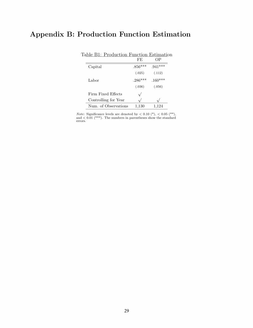
Appendix B: Production Function Estimation
Table B1: Production Function EstimationFE OP
Capital .856*** .941***
(.025) (.112)
Labor .286*** .160***
(.036) (.056)
Firm Fixed Effects√
Controlling for Year√ √
Num. of Observations 1,130 1,124
Note: Significance levels are denoted by < 0.10 (*), < 0.05 (**),and < 0.01 (***). The numbers in parentheses show the standarderrors.
29


