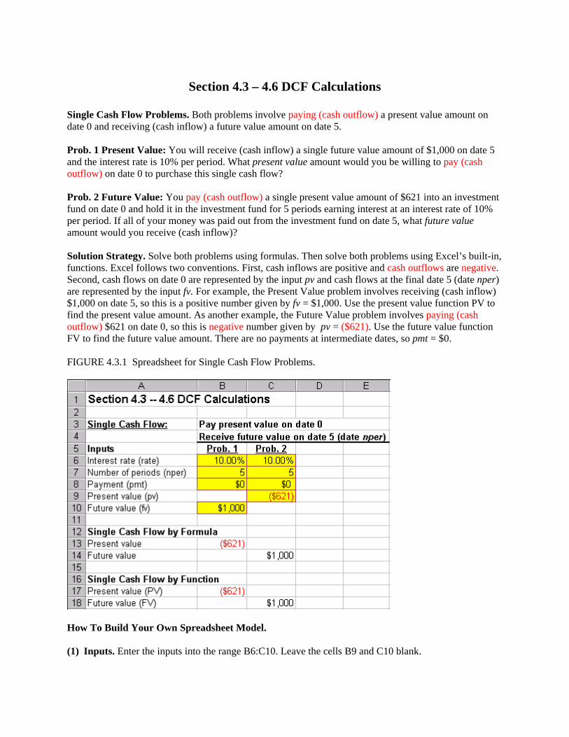
Section 4.3 – 4.6 DCF Calculations

Single Cash Flow Problems. Both problems involve paying (cash outflow) a present value amount on date 0 and receiving (cash inflow) a future value amount on date 5. Prob. 1 Present Value: You will receive (cash inflow) a single future value amount of $1,000 on date 5 and the interest rate is 10% per period. What present value amount would you be willing to pay (cash outflow) on date 0 to purchase this single cash flow? Prob. 2 Future Value: You pay (cash outflow) a single present value amount of $621 into an investment fund on date 0 and hold it in the investment fund for 5 periods earning interest at an interest rate of 10% per period. If all of your money was paid out from the investment fund on date 5, what future value amount would you receive (cash inflow)? Solution Strategy. Solve both problems using formulas. Then solve both problems using Excel’s built-in, functions. Excel follows two conventions. First, cash inflows are positive and cash outflows are negative. Second, cash flows on date 0 are represented by the input pv and cash flows at the final date 5 (date nper) are represented by the input fv. For example, the Present Value problem involves receiving (cash inflow) $1,000 on date 5, so this is a positive number given by fv = $1,000. Use the present value function PV to find the present value amount. As another example, the Future Value problem involves paying (cash outflow) $621 on date 0, so this is negative number given by pv = ($621). Use the future value function FV to find the future value amount. There are no payments at intermediate dates, so pmt = $0. FIGURE 4.3.1 Spreadsheet for Single Cash Flow Problems.

How To Build Your Own Spreadsheet Model.

) Inputs. Enter the inputs into the range B6:C10. Leave the cells B9 and C10 blank.

(1

(2) Present Value by Formula. Using Excel’s sign convention, the formula for the present value of a single cash flow in the future is

( )( )nperrate

fvPV+

−=

1

Enter =(-B10)/((1+B6)^B7) in cell B13. (3) Future Value by Formula. Using Excel’s sign convention, the formula for the future value of a

single cash flow in the future is ( )( )nperratepvFV +−= 1

Enter =(-C9)*((1+C6)^C7) in cell C14. (4) Present Value by Function. The format for using the present value function is PV(rate,nper,pmt,fv).

Enter =PV(B6,B7,B8,B10) in cell B17. (5) Future Value by Function. The format for using the future value function is FV(rate,nper,pmt,pv).

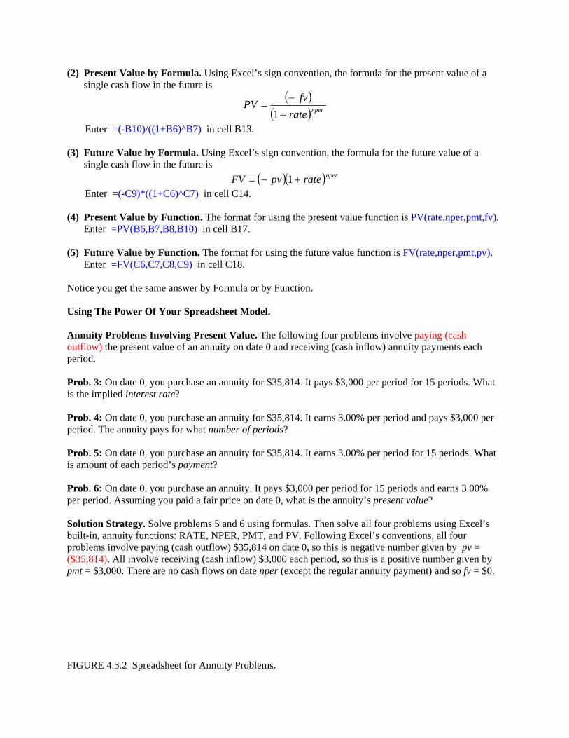
Enter =FV(C6,C7,C8,C9) in cell C18. Notice you get the same answer by Formula or by Function. Using The Power Of Your Spreadsheet Model. Annuity Problems Involving Present Value. The following four problems involve paying (cash outflow) the present value of an annuity on date 0 and receiving (cash inflow) annuity payments each period. Prob. 3: On date 0, you purchase an annuity for $35,814. It pays $3,000 per period for 15 periods. What is the implied interest rate? Prob. 4: On date 0, you purchase an annuity for $35,814. It earns 3.00% per period and pays $3,000 per period. The annuity pays for what number of periods? Prob. 5: On date 0, you purchase an annuity for $35,814. It earns 3.00% per period for 15 periods. What is amount of each period’s payment? Prob. 6: On date 0, you purchase an annuity. It pays $3,000 per period for 15 periods and earns 3.00% per period. Assuming you paid a fair price on date 0, what is the annuity’s present value? Solution Strategy. Solve problems 5 and 6 using formulas. Then solve all four problems using Excel’s built-in, annuity functions: RATE, NPER, PMT, and PV. Following Excel’s conventions, all four problems involve paying (cash outflow) $35,814 on date 0, so this is negative number given by pv = ($35,814). All involve receiving (cash inflow) $3,000 each period, so this is a positive number given by pmt = $3,000. There are no cash flows on date nper (except the regular annuity payment) and so fv = $0. FIGURE 4.3.2 Spreadsheet for Annuity Problems.

1. Inputs. Enter the inputs into the range B24:E28. Leave the diagonal cells B24, C25, D26, and E27

blank. 2. Payment by Formula. Using Excel’s sign convention, the formula for the annuity’s payment is

( )( )

rateratepvPMT nper−+−

−=

11

Enter =(-D27)/((1-((1+D24)^(-D25)))/D24) in cell D33. 3. Present Value by Formula. Using Excel’s sign convention, the formula for the annuity’s present

value is

( ) ( )⎟⎟⎠

⎞⎜⎜⎝

⎛ +−−=

−

rateratepmtPV

nper11

Enter =(-E26)*(1-((1+E24)^(-E25)))/E24 in cell E34. 4. Annuity Functions. Solve all four-related problems by using the built-in, annuity functions

• Calculate the interest rate by entering =RATE(B25,B26,B27,B28) in cell B38. • Calculate the number of periods by entering =NPER(C24,C26,C27,C28) in cell C39. • Calculate the payment by entering =PMT(D24,D25,D27,D28) in cell D40. • Calculate the present value by entering =PV(E24,E25,E26,E28) in cell E41.

Notice you get the same answers by Formula or by Function.

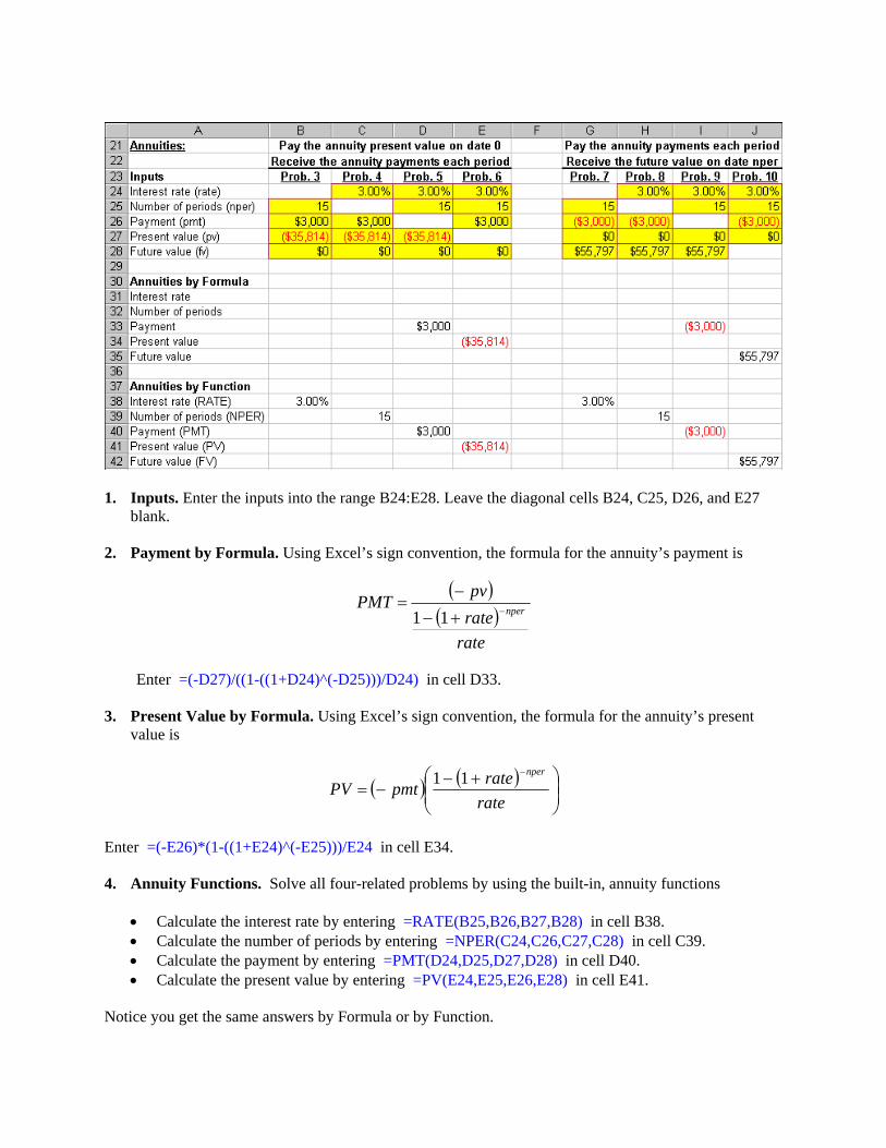
Annuity Problems Involving FutureValue. Here are four additional annuity problems that all involvepaying (cash outflow) annuity payments each period into an investment fund, earning the interest rate each period, and r

eceiving (cash inflow) the future value of the annuity on date 15 (date nper) from the vestment fund.

3,000 per period for 15 periods. On date nper, receive $55,797. What is the implied terest rate?

nd earn 3.00% per period. On date nper, receive 55,797. The annuity pays for what number of periods?

nd earn 3.00% per period. On date nper, receive 55,797. What is amount of each period’s payment?

0% per period. ssuming you receive a fair value on date nper, what is the annuity’s future value?

y ), so this is a positive

umber given by fv = $55,797. There are no cash flows on date 0 and so pv = $0.

. Inputs. Enter the inputs into the range G24:J28 Leave the cells G24, H25, I26, and J28 blank.

ayment by Formula. Using Excel’s sign convention, the formula for the annuity’s payment is

in Prob. 7: Pay $in Prob. 8: Pay $3,000 per period into an investment fund a$ Prob. 9: Pay into an investment fund for 15 periods a$ Prob. 10: Pay $3,000 per period into an investment fund for 15 periods and earn 3.0A Solution Strategy. Solve problems 9 and 10 using formulas. Then solve all of the new problems using Excel’s built-in, annuity functions: RATE, NPER, PMT, and FV. Following Excel conventions, all four-related problems involve paying (cash outflow) $3,000 each period, so this is a negative number given bpmt = ($3,000). All involve receiving (cash inflow) $55,797 on date 15 (date npern 1 2. P

( )( )

raterate

fvPMT nper 11 −+

−=

Enter =(-I28)/((((1+I24)^I25)-1)/I24) in cell I33.

3. alue by Formula. Using Excel’s sign convention, the formula for the annuity’s present lue is

Future Vva

( ) ( )⎟⎟⎠

⎞⎜⎜⎝

⎛ −+−=

rateratepmtFV

nper 11

Enter =(-J26)*(((1+J24)^J25)-1)/J24 in cell J35.

. Annuity Functions. Solve all four-related problems by using the built-in, annuity functions

) in cell H39.

• Calculate the future value by entering =FV(J24,J25,J26,J27) in cell J42.

4

• Calculate the interest rate by entering =RATE(G25,G26,G27,G28) in cell G38. • Calculate the number of periods by entering =NPER(H24,H26,H27,H28• Calculate the payment by entering =PMT(I24,I25,I27,I28) in cell I40.

Notice you get the same answers by Formula or by Function.

low) annuity payments each period, and receiving (cash inflow) a xed payment on date 20 (date nper).

ceive $30 per period for 20 periods, and receive $10,000 on ate nper. What is the implied interest rate?

earn 4.00% per period, and receive 10,000 on date nper. The bond pays for what number of periods?

ds, earn 4.00% per eriod, and receive $10,000 on date nper. What is amount of each period’s payment?

20 periods, arn 4.00% per period, and receive $10,000 on date nper. What is the bond’s present value?

0% per period, nd receive the appropriate fixed payment on date nper. What is the bond’s future value?

IGURE 4.3.3 Spreadsheet for Bond Problems.

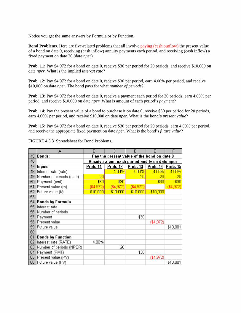
Bond Problems. Here are five-related problems that all involve paying (cash outflow) the present value of a bond on date 0, receiving (cash inffi Prob. 11: Pay $4,972 for a bond on date 0, red Prob. 12: Pay $4,972 for a bond on date 0, receive $30 per period, $ Prob. 13: Pay $4,972 for a bond on date 0, receive a payment each period for 20 periop Prob. 14: Pay the present value of a bond to purchase it on date 0, receive $30 per period fore Prob. 15: Pay $4,972 for a bond on date 0, receive $30 per period for 20 periods, earn 4.0a F

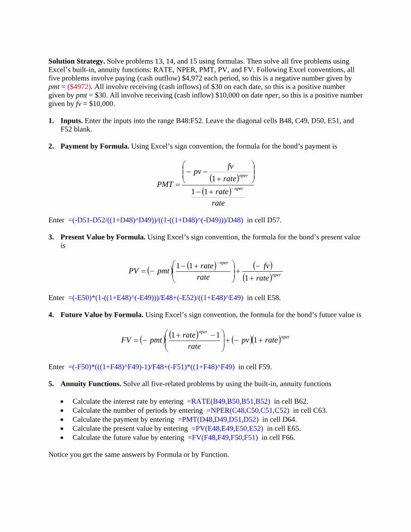
Solution Strategy. Solve problems 13, 14, and 15 using formulas. Then solve all five problems usingExcel’s built-in, annuity functions: RATE, NPER, PMT, PV, and FV. Following Excel conventions, all five problems involve p

aying (cash outflow) $4,972 each period, so this is a negative number given by mt = ($4972). All involve receiving (cash inflows) of $30 on each date, so this is a positive number

r giv 0,000.

and 52 blank.

2. Payment by Formula. Using Excel’s sign convention, the formula for the bond’s payment is

pgiven by pmt = $30. All involve receiving (cash inflow) $10,000 on date nper, so this is a positive numbe

en by fv = $1 1. Inputs. Enter the inputs into the range B48:F52. Leave the diagonal cells B48, C49, D50, E51,

F

( )( )

rate

ratefvpv

PMTnper ⎟⎟

⎠

⎞⎜⎜⎝

⎛

+−−

=1

Ent 1-((1+D48)^(-D49)))/D48) in cell D57.

3. Present Value by Formula. Using Excel’s sign convention, the formula for the bond’s present value is

rate nper−+− 11

er =(-D51-D52/((1+D48)^D49))/((

( ) ( ) ( )( )nperrate

fvrateratepmtPV

++⎟⎟⎜⎜−=

111 nper −

⎠

⎞

⎝

⎛ +− −

=(-E50)*(1-((1+E48)^(-E49)))/E48+(-E52)/((1+E48)^E49) in cell E58. 4. Future Value by Formula. Using Excel’s sign convention, the formula for the bond’s future value is

Enter

( ) ( ) ( )( ratepvrate

ratepmtFV +−+⎟⎟⎜⎜−= 111 )npernper

⎠

⎞

⎝

⎛ −+

nter =(-F50)*(((1+F48)^F49)-1)/F48+(-F51)*((1+F48)^F49) in cell F59. 5.

. cell C63.

• Calculate the payment by entering =PMT(D48,D49,D51,D52) in cell D64. ,E50,E52) in cell E65.

• Calculate the future value by entering =FV(F48,F49,F50,F51) in cell F66. Notice you get the same answers by Formula or by Function.

E

Annuity Functions. Solve all five-related problems by using the built-in, annuity functions

• Calculate the interest rate by entering =RATE(B49,B50,B51,B52) in cell B62• Calculate the number of periods by entering =NPER(C48,C50,C51,C52) in

• Calculate the present value by entering =PV(E48,E49

Section 4.8 Mortgage Loan Amortization

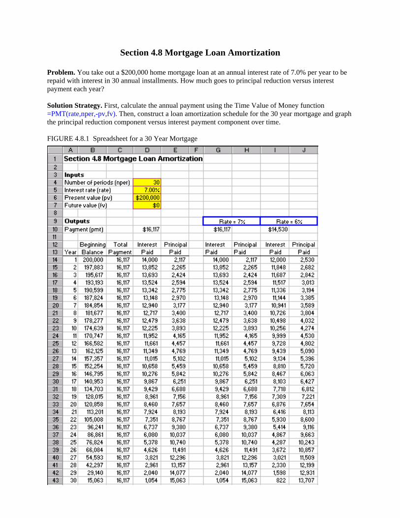
Problem. You take out a $200,000 home mortgage loan at an annual interest rate of 7.0% per year to be repaid with interest in 30 annual installments. How much goes to principal reduction versus interest payment each year? Solution Strategy. First, calculate the annual payment using the Time Value of Money function =PMT(rate,nper,-pv,fv). Then, construct a loan amortization schedule for the 30 year mortgage and graph the principal reduction component versus interest payment component over time. FIGURE 4.8.1 Spreadsheet for a 30 Year Mortgage

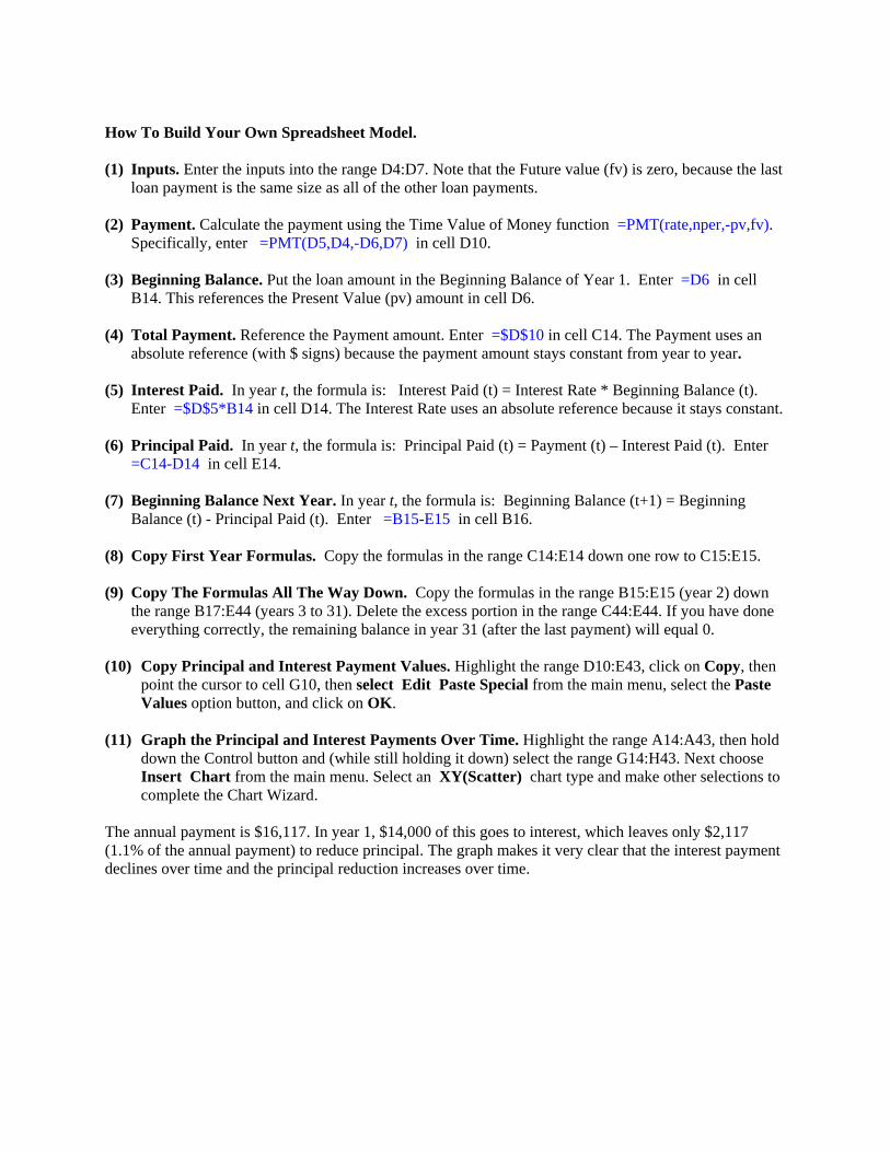
How To Build Your Own Spreadsheet Model. (1) Inputs. Enter the inputs into the range D4:D7. Note that the Future value (fv) is zero, because the last

loan payment is the same size as all of the other loan payments. (2) Payment. Calculate the payment using the Time Value of Money function =PMT(rate,nper,-pv,fv).

Specifically, enter =PMT(D5,D4,-D6,D7) in cell D10. (3) Beginning Balance. Put the loan amount in the Beginning Balance of Year 1. Enter =D6 in cell

B14. This references the Present Value (pv) amount in cell D6. (4) Total Payment. Reference the Payment amount. Enter =$D$10 in cell C14. The Payment uses an

absolute reference (with $ signs) because the payment amount stays constant from year to year. (5) Interest Paid. In year t, the formula is: Interest Paid (t) = Interest Rate * Beginning Balance (t).

Enter =$D$5*B14 in cell D14. The Interest Rate uses an absolute reference because it stays constant. (6) Principal Paid. In year t, the formula is: Principal Paid (t) = Payment (t) – Interest Paid (t). Enter

=C14-D14 in cell E14. (7) Beginning Balance Next Year. In year t, the formula is: Beginning Balance (t+1) = Beginning

Balance (t) - Principal Paid (t). Enter =B15-E15 in cell B16. (8) Copy First Year Formulas. Copy the formulas in the range C14:E14 down one row to C15:E15. (9) Copy The Formulas All The Way Down. Copy the formulas in the range B15:E15 (year 2) down

the range B17:E44 (years 3 to 31). Delete the excess portion in the range C44:E44. If you have done everything correctly, the remaining balance in year 31 (after the last payment) will equal 0.

(10) Copy Principal and Interest Payment Values. Highlight the range D10:E43, click on Copy, then

point the cursor to cell G10, then select Edit Paste Special from the main menu, select the Paste Values option button, and click on OK.

(11) Graph the Principal and Interest Payments Over Time. Highlight the range A14:A43, then hold

down the Control button and (while still holding it down) select the range G14:H43. Next choose Insert Chart from the main menu. Select an XY(Scatter) chart type and make other selections to complete the Chart Wizard.

The annual payment is $16,117. In year 1, $14,000 of this goes to interest, which leaves only $2,117 (1.1% of the annual payment) to reduce principal. The graph makes it very clear that the interest payment declines over time and the principal reduction increases over time.

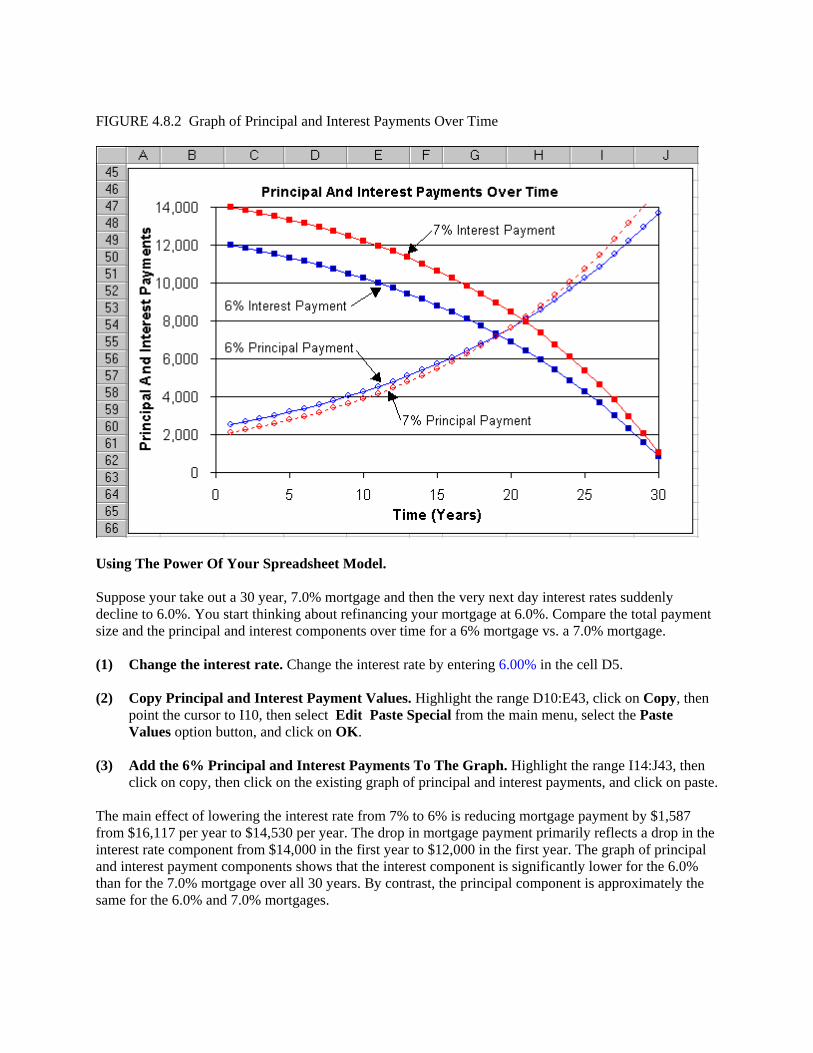
FIGURE 4.8.2 Graph of Principal and Interest Payments Over Time

Using The Power Of Your Spreadsheet Model. Suppose your take out a 30 year, 7.0% mortgage and then the very next day interest rates suddenly decline to 6.0%. You start thinking about refinancing your mortgage at 6.0%. Compare the total payment size and the principal and interest components over time for a 6% mortgage vs. a 7.0% mortgage. (1) Change the interest rate. Change the interest rate by entering 6.00% in the cell D5. (2) Copy Principal and Interest Payment Values. Highlight the range D10:E43, click on Copy, then

point the cursor to I10, then select Edit Paste Special from the main menu, select the Paste Values option button, and click on OK.

(3) Add the 6% Principal and Interest Payments To The Graph. Highlight the range I14:J43, then

click on copy, then click on the existing graph of principal and interest payments, and click on paste. The main effect of lowering the interest rate from 7% to 6% is reducing mortgage payment by $1,587 from $16,117 per year to $14,530 per year. The drop in mortgage payment primarily reflects a drop in the interest rate component from $14,000 in the first year to $12,000 in the first year. The graph of principal and interest payment components shows that the interest component is significantly lower for the 6.0% than for the 7.0% mortgage over all 30 years. By contrast, the principal component is approximately the same for the 6.0% and 7.0% mortgages.

Section 4.10 Inflation and DCF Calculations

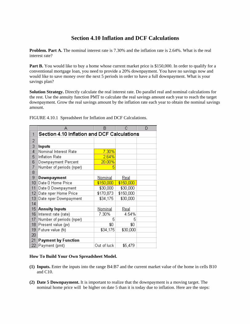
Problem. Part A. The nominal interest rate is 7.30% and the inflation rate is 2.64%. What is the real interest rate? Part B. You would like to buy a home whose current market price is $150,000. In order to qualify for a conventional mortgage loan, you need to provide a 20% downpayment. You have no savings now and would like to save money over the next 5 periods in order to have a full downpayment. What is your savings plan? Solution Strategy. Directly calculate the real interest rate. Do parallel real and nominal calculations for the rest. Use the annuity function PMT to calculate the real savings amount each year to reach the target downpayment. Grow the real savings amount by the inflation rate each year to obtain the nominal savings amount. FIGURE 4.10.1 Spreadsheet for Inflation and DCF Calculations.

How To Build Your Own Spreadsheet Model. (1) Inputs. Enter the inputs into the range B4:B7 and the current market value of the home in cells B10

and C10. (2) Date 5 Downpayment. It is important to realize that the downpayment is a moving target. The

nominal home price will be higher on date 5 than it is today due to inflation. Here are the steps:

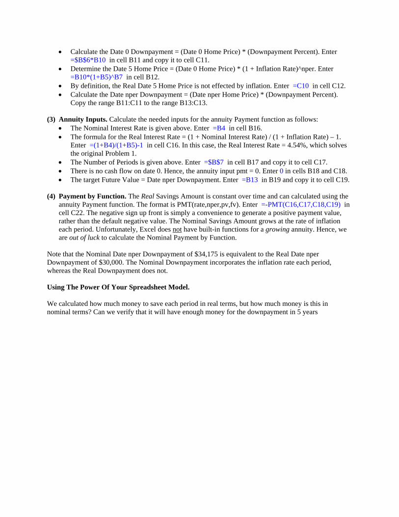
• Calculate the Date 0 Downpayment = (Date 0 Home Price) * (Downpayment Percent). Enter =$B$6*B10 in cell B11 and copy it to cell C11.

• Determine the Date 5 Home Price = (Date 0 Home Price) * (1 + Inflation Rate)^nper. Enter =B10*(1+B5)^B7 in cell B12.

• By definition, the Real Date 5 Home Price is not effected by inflation. Enter =C10 in cell C12. • Calculate the Date nper Downpayment = (Date nper Home Price) * (Downpayment Percent).

Copy the range B11:C11 to the range B13:C13.

(3) Annuity Inputs. Calculate the needed inputs for the annuity Payment function as follows: • The Nominal Interest Rate is given above. Enter =B4 in cell B16. • The formula for the Real Interest Rate = (1 + Nominal Interest Rate) / (1 + Inflation Rate) – 1.

Enter =(1+B4)/(1+B5)-1 in cell C16. In this case, the Real Interest Rate = 4.54%, which solves the original Problem 1.

• The Number of Periods is given above. Enter =$B$7 in cell B17 and copy it to cell C17. • There is no cash flow on date 0. Hence, the annuity input pmt = 0. Enter 0 in cells B18 and C18. • The target Future Value = Date nper Downpayment. Enter =B13 in B19 and copy it to cell C19.

(4) Payment by Function. The Real Savings Amount is constant over time and can calculated using the

annuity Payment function. The format is PMT(rate,nper,pv,fv). Enter =-PMT(C16,C17,C18,C19) in cell C22. The negative sign up front is simply a convenience to generate a positive payment value, rather than the default negative value. The Nominal Savings Amount grows at the rate of inflation each period. Unfortunately, Excel does not have built-in functions for a growing annuity. Hence, we are out of luck to calculate the Nominal Payment by Function.

Note that the Nominal Date nper Downpayment of $34,175 is equivalent to the Real Date nper Downpayment of $30,000. The Nominal Downpayment incorporates the inflation rate each period, whereas the Real Downpayment does not. Using The Power Of Your Spreadsheet Model. We calculated how much money to save each period in real terms, but how much money is this in nominal terms? Can we verify that it will have enough money for the downpayment in 5 years

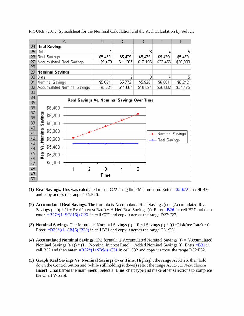
FIGURE 4.10.2 Spreadsheet for the Nominal Calculation and the Real Calculation by Solver.

(1) Real Savings. This was calculated in cell C22 using the PMT function. Enter =$C$22 in cell B26

and copy across the range C26:F26. (2) Accumulated Real Savings. The formula is Accumulated Real Savings (t) = (Accumulated Real

Savings (t-1)) * (1 + Real Interest Rate) + Added Real Savings (t). Enter =B26 in cell B27 and then enter =B27*(1+$C$16)+C26 in cell C27 and copy it across the range D27:F27.

(3) Nominal Savings. The formula is Nominal Savings (t) = Real Savings (t) * ((1+Riskfree Rate) ^ t)

Enter =B26*((1+$B$5)^B30) in cell B31 and copy it across the range C31:F31. (4) Accumulated Nominal Savings. The formula is Accumulated Nominal Savings (t) = (Accumulated

Nominal Savings (t-1)) * (1 + Nominal Interest Rate) + Added Nominal Savings (t). Enter =B31 in cell B32 and then enter =B32*(1+$B$4)+C31 in cell C32 and copy it across the range D32:F32.

(5) Graph Real Savings Vs. Nominal Savings Over Time. Highlight the range A26:F26, then hold

down the Control button and (while still holding it down) select the range A31:F31. Next choose Insert Chart from the main menu. Select a Line chart type and make other selections to complete the Chart Wizard.

The Nominal Savings amount in Row 31 shows the actual nominal savings amount that one needs to save each period. Notice that the Accumulated Real Savings adds up to $30,000, which is the Date 5 Downpayment in Real Terms. Further, the Accumulated Nominal Savings adds up to $34,175, which is the Date 5 Downpayment in Nominal Terms. The graph shows that the Nominal Savings amount goes up each year reflecting inflation increases each year. By contrast, the Real Savings amount stays constant each year reflecting a constant level of real consumption that must be sacrificed in order to generate this level of savings.

Section 6.3 Net Present Value

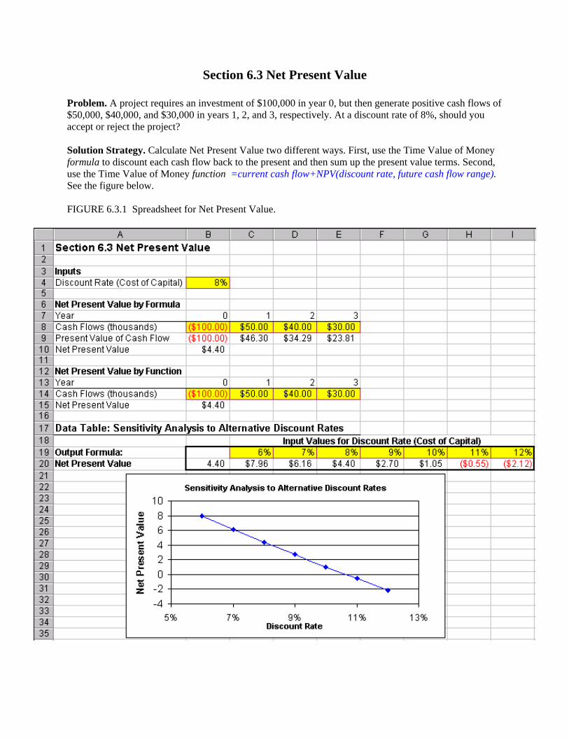
Problem. A project requires an investment of $100,000 in year 0, but then generate positive cash flows of $50,000, $40,000, and $30,000 in years 1, 2, and 3, respectively. At a discount rate of 8%, should you accept or reject the project? Solution Strategy. Calculate Net Present Value two different ways. First, use the Time Value of Money formula to discount each cash flow back to the present and then sum up the present value terms. Second, use the Time Value of Money function =current cash flow+NPV(discount rate, future cash flow range). See the figure below. FIGURE 6.3.1 Spreadsheet for Net Present Value.

How To Build Your Own Spreadsheet Model. (1) Inputs. Enter the Discount Rate in cell B4, the year-by-year Cash Flows in the range B8:E8, and the

same Cash Flows in the range B4:B7. Note that the Year 0 cash flow is negative, because it represents a cash outflow.

(2) Net Present Value by Formula. Calculate the present value of the cash flows by entering the Time

Value of Money formula =B8/((1+$B$4)^B7) in cell B9. Copy this formula from cell B9 across the range C9:E9. The Discount Rate $B$4 uses an absolute reference because it stays constant from year to year. For convenience, the number of times to compound B7 is taken from the year number. Calculate Net Present Value by summing all of the present value of cash flow terms. Enter =SUM(B9:E9) in cell B10.

(3) Net Present Value by Function. Calculate Net Present Value by using the Time Value of Money

function =current cash flow + NPV(discount rate, future cash flow range). Enter =B14+NPV(B4,C14:E14) in cell B15. Note that the NPV function assumes that future case flows start in year 1, so the current (year 0) cash flow must be added separately.

The Net Present Value is positive, so the project should be accepted. Notice you get the same answer by formula or by function! Using The Power Of Your Spreadsheet Model. Suppose your not sure about the exact discount rate. You can test the sensitivity of the project NPV to the discount rate. (1) Create A List of Input Values and An Output Formula. Create a list of input values for the

Discount Rate (6%, 7%, 8%, etc.) in the range C19:I19. Create an output formula that references the product NPV by entering the formula =B15 in cell B20.

(2) Data Table. Select the range B19:I20 for the Data Table. This range includes both the list of input

values at the top of the data table and the output formula on the side of the data table. Then choose Data Table from the main menu and a Table dialog box pops up. Enter the cell address B4 (for the Discount Rate) in the Row Input Cell and click on OK.

(3) Graph the Sensitivity Analysis. Highlight the data table C19:I20 and then choose Insert Chart

from the main menu. Select an XY(Scatter) chart type and make other selections to complete the Chart Wizard.

The sensitivity analysis shows that the NPV is positive over a wide range of discount rates (6% - 10%) and doesn’t go negative until 11% or above. This should inspire confidence that the calculation of a positive NPV for the project is a robust result.

Section 8.4 Reading Bond Listings

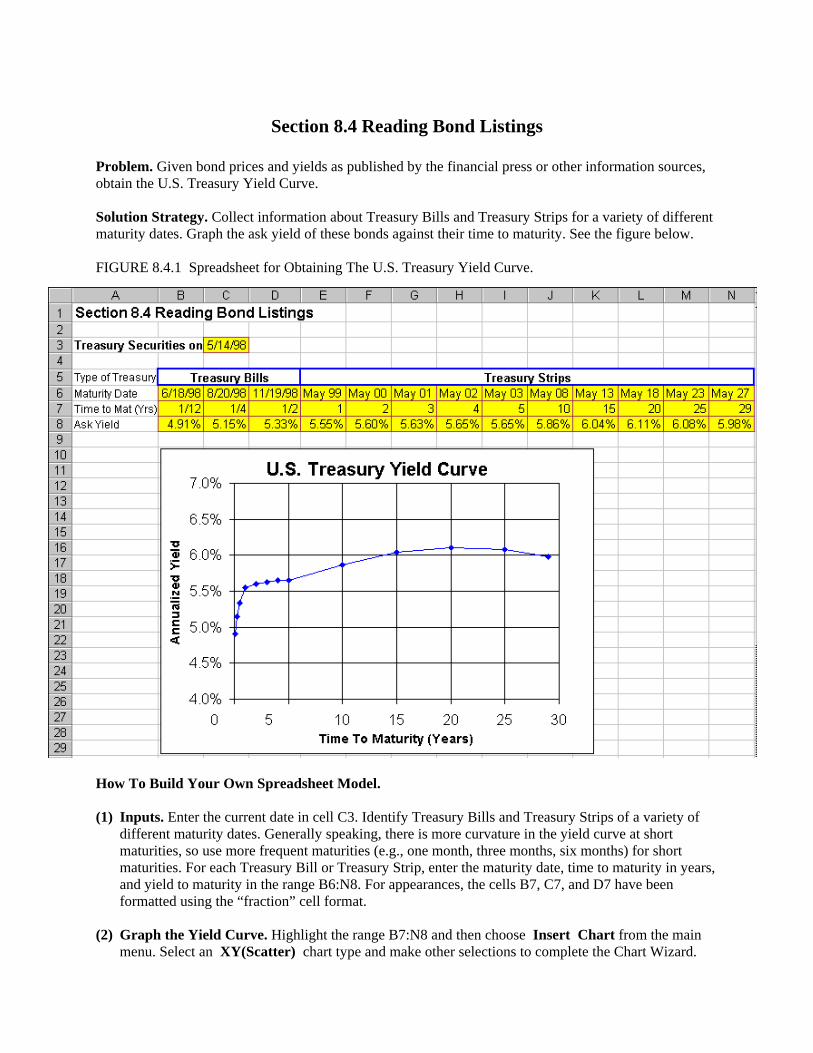
Problem. Given bond prices and yields as published by the financial press or other information sources, obtain the U.S. Treasury Yield Curve. Solution Strategy. Collect information about Treasury Bills and Treasury Strips for a variety of different maturity dates. Graph the ask yield of these bonds against their time to maturity. See the figure below. FIGURE 8.4.1 Spreadsheet for Obtaining The U.S. Treasury Yield Curve.

How To Build Your Own Spreadsheet Model. (1) Inputs. Enter the current date in cell C3. Identify Treasury Bills and Treasury Strips of a variety of

different maturity dates. Generally speaking, there is more curvature in the yield curve at short maturities, so use more frequent maturities (e.g., one month, three months, six months) for short maturities. For each Treasury Bill or Treasury Strip, enter the maturity date, time to maturity in years, and yield to maturity in the range B6:N8. For appearances, the cells B7, C7, and D7 have been formatted using the “fraction” cell format.

(2) Graph the Yield Curve. Highlight the range B7:N8 and then choose Insert Chart from the main

menu. Select an XY(Scatter) chart type and make other selections to complete the Chart Wizard.

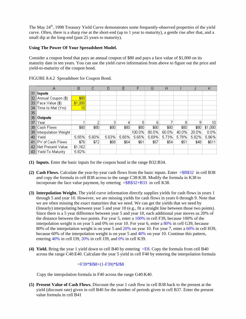
The May 24th, 1998 Treasury Yield Curve demonstrates some frequently-observed properties of the yield curve. Often, there is a sharp rise at the short-end (up to 1 year to maturity), a gentle rise after that, and a small dip at the long-end (past 25 years to maturity). Using The Power Of Your Spreadsheet Model. Consider a coupon bond that pays an annual coupon of $80 and pays a face value of $1,000 on its maturity date in ten years. You can use the yield curve information from above to figure out the price and yield-to-maturity of the coupon bond. FIGURE 8.4.2 Spreadsheet for Coupon Bond.

(1) Inputs. Enter the basic inputs for the coupon bond in the range B32:B34. (2) Cash Flows. Calculate the year-by-year cash flows from the basic inputs. Enter =$B$32 in cell B38

and copy the formula in cell B38 across to the range C38:K38. Modify the formula in K38 to incorporate the face value payment, by entering =$B$32+B33 in cell K38.

(3) Interpolation Weight. The yield curve information directly supplies yields for cash flows in years 1

through 5 and year 10. However, we are missing yields for cash flows in years 6 through 9. Note that we are often missing the exact maturities that we need. We can get the yields that we need by (linearly) interpolating between year 5 and year 10 (e.g., fit a straight line between those two points). Since there is a 5 year difference between year 5 and year 10, each additional year moves us 20% of the distance between the two points. For year 5, enter a 100% in cell F39, because 100% of the interpolation weight is on year 5 and 0% on year 10. For year 6, enter a 80% in cell G39, because 80% of the interpolation weight is on year 5 and 20% on year 10. For year 7, enter a 60% in cell H39, because 60% of the interpolation weight is on year 5 and 40% on year 10. Continue this pattern, entering 40% in cell I39, 20% in cell J39, and 0% in cell K39.

(4) Yield. Bring the year 1 yield down to cell B40 by entering =E8. Copy the formula from cell B40

across the range C40:E40. Calculate the year 5 yield in cell F40 by entering the interpolation formula =F39*$I$8+(1-F39)*$J$8 Copy the interpolation formula in F40 across the range G40:K40. (5) Present Value of Cash Flows. Discount the year 1 cash flow in cell B38 back to the present at the

yield (discount rate) given in cell B40 for the number of periods given in cell B37. Enter the present value formula in cell B41

=B38/((1+B40)^B37) Copy the present value formula in B41 across the range C41:K41. (6) Net Present Value. Sum up the present value of all of the cash flows in cell B42 by entering =SUM(B41:K41) (7) Yield To Maturity. The yield to maturity for the coupon bond can be calculated using the annuity

function =RATE(nper,pmt,-pv,fv). In cell B43, enter =RATE(B34,B32,-B42,B33) The coupon bond has a price of $1,162 and a yield to maturity of 5.82%. Notice that this yield to maturity is much closer to the year 10 yield of 5.86% than it is to the year 1 yield of 5.55%. This is because there is a much bigger cash flow in year 10 ($1,080) than in year 1 ($80), which heavily weights the overall yield to maturity towards the year 10 yield.

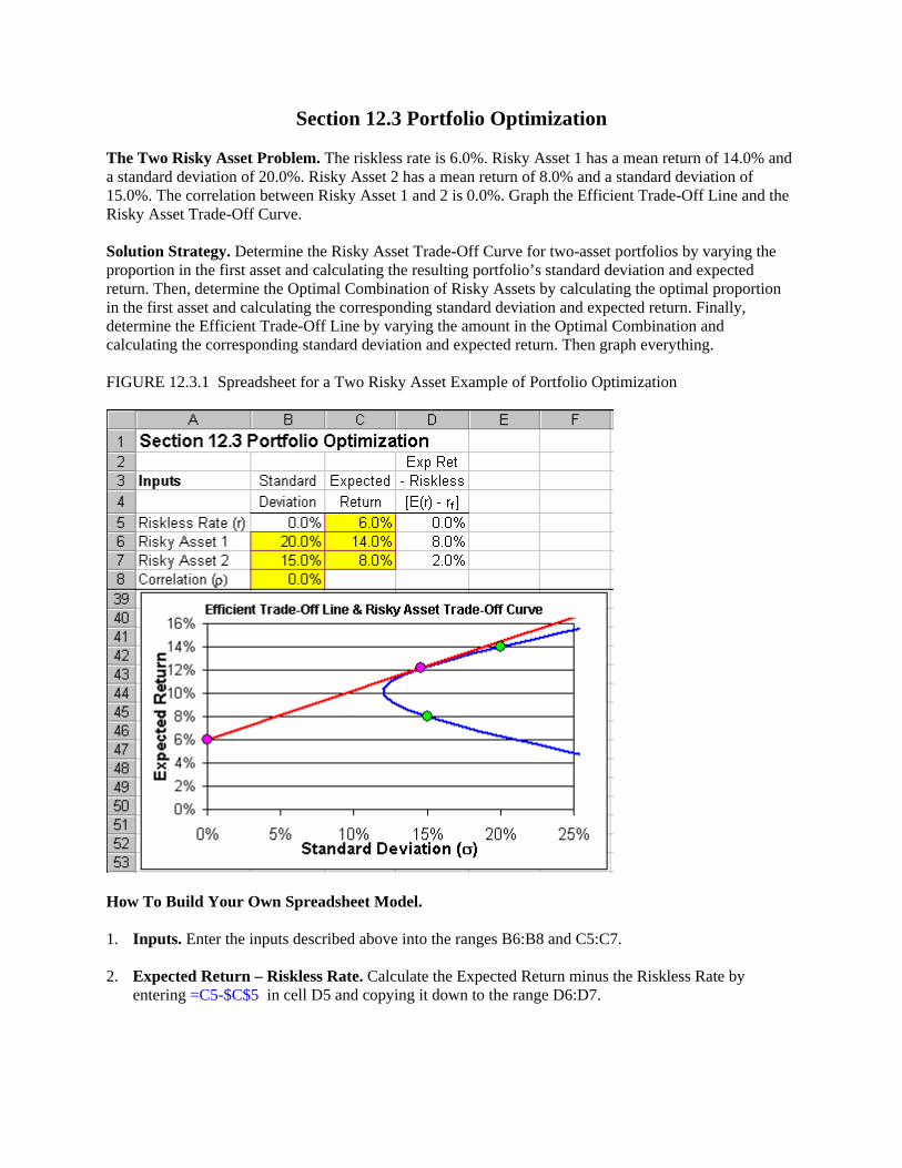
Section 12.3 Portfolio Optimization The Two Risky Asset Problem. The riskless rate is 6.0%. Risky Asset 1 has a mean return of 14.0% and a standard deviation of 20.0%. Risky Asset 2 has a mean return of 8.0% and a standard deviation of 15.0%. The correlation between Risky Asset 1 and 2 is 0.0%. Graph the Efficient Trade-Off Line and the Risky Asset Trade-Off Curve. Solution Strategy. Determine the Risky Asset Trade-Off Curve for two-asset portfolios by varying the proportion in the first asset and calculating the resulting portfolio’s standard deviation and expected return. Then, determine the Optimal Combination of Risky Assets by calculating the optimal proportion in the first asset and calculating the corresponding standard deviation and expected return. Finally, determine the Efficient Trade-Off Line by varying the amount in the Optimal Combination and calculating the corresponding standard deviation and expected return. Then graph everything. FIGURE 12.3.1 Spreadsheet for a Two Risky Asset Example of Portfolio Optimization

How To Build Your Own Spreadsheet Model. 1. Inputs. Enter the inputs described above into the ranges B6:B8 and C5:C7. 2. Expected Return – Riskless Rate. Calculate the Expected Return minus the Riskless Rate by

entering =C5-$C$5 in cell D5 and copying it down to the range D6:D7.

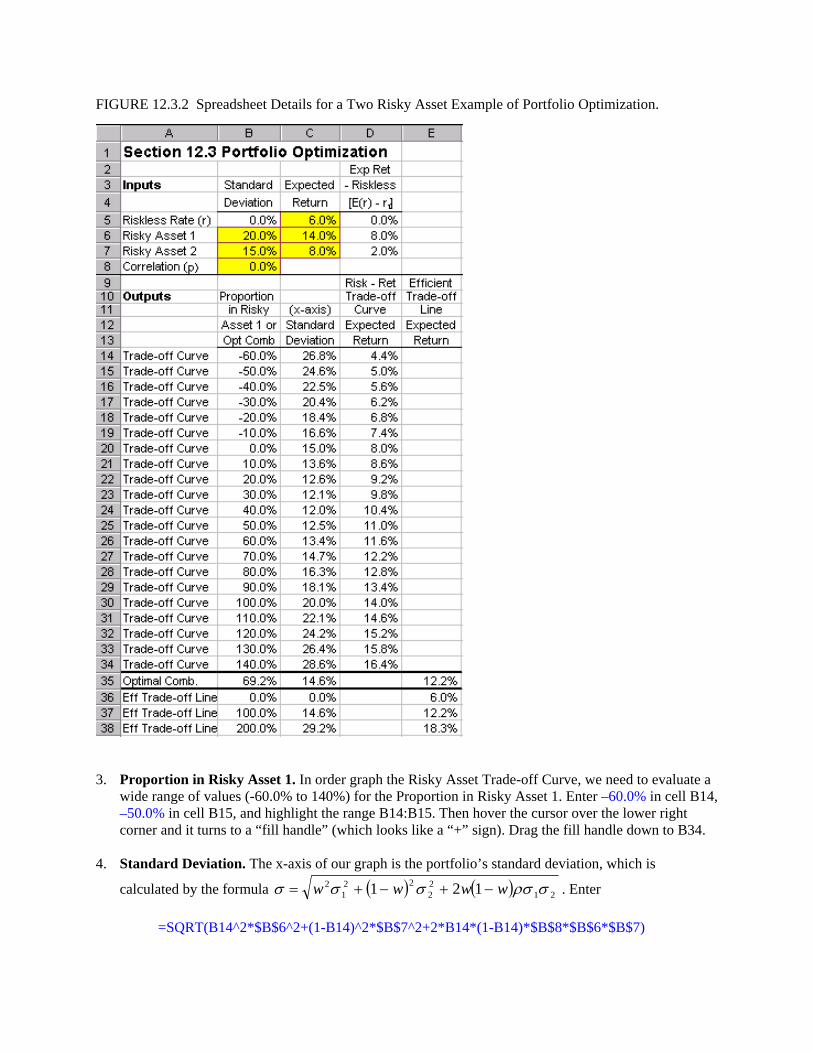
FIGURE 12.3.2 Spreadsheet Details for a Two Risky Asset Example of Portfolio Optimization.

3. Proportion in Risky Asset 1. In order graph the Risky Asset Trade-off Curve, we need to evaluate a

wide range of values (-60.0% to 140%) for the Proportion in Risky Asset 1. Enter –60.0% in cell B14, –50.0% in cell B15, and highlight the range B14:B15. Then hover the cursor over the lower right corner and it turns to a “fill handle” (which looks like a “+” sign). Drag the fill handle down to B34.

4. Standard Deviation. The x-axis of our graph is the portfolio’s standard deviation, which is

calculated by the formula ( ) ( ) 2122

221

2 121 σρσσσσ wwww −+−+= . Enter =SQRT(B14^2*$B$6^2+(1-B14)^2*$B$7^2+2*B14*(1-B14)*$B$8*$B$6*$B$7)

in cell C14 and copy the cell C14 to the range C15:C34. 5. Expected Return. The formula for a portfolio’s expected return is ( ) ( ) ( ) ( )21 1 rEwrwErE −+= .

Enter =B14*$C$6+(1-B14)*$C$7 in cell D14 and copy the cell D14 to the range D15:D34. 6. Optimal Combination of Risky Assets. Using the notation that ( ) frrEE −= 11 and

, then the formula for the optimal proportion in the first asset is ( ) frrEE −= 22

( ) ( )( )212212

221212

2211 / σρσσσσρσσ EEEEEEw −+−= . In cell B35, enter

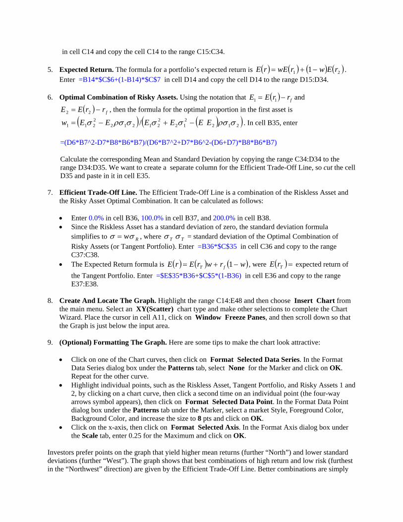
=(D6*B7^2-D7*B8*B6*B7)/(D6*B7^2+D7*B6^2-(D6+D7)*B8*B6*B7) Calculate the corresponding Mean and Standard Deviation by copying the range C34:D34 to the range D34:D35. We want to create a separate column for the Efficient Trade-Off Line, so cut the cell D35 and paste in it in cell E35. 7. Efficient Trade-Off Line. The Efficient Trade-Off Line is a combination of the Riskless Asset and

the Risky Asset Optimal Combination. It can be calculated as follows:

• Enter 0.0% in cell B36, 100.0% in cell B37, and 200.0% in cell B38. • Since the Riskless Asset has a standard deviation of zero, the standard deviation formula

simplifies to Rwσσ = , where Tσ σ T = standard deviation of the Optimal Combination of Risky Assets (or Tangent Portfolio). Enter =B36*$C$35 in cell C36 and copy to the range C37:C38.

• The Expected Return formula is ( ) ( ) ( )wrwrErE fT −+= 1 , were ( ) =TrE expected return of the Tangent Portfolio. Enter =$E$35*B36+$C$5*(1-B36) in cell E36 and copy to the range E37:E38.

8. Create And Locate The Graph. Highlight the range C14:E48 and then choose Insert Chart from

the main menu. Select an XY(Scatter) chart type and make other selections to complete the Chart Wizard. Place the cursor in cell A11, click on Window Freeze Panes, and then scroll down so that the Graph is just below the input area.

9. (Optional) Formatting The Graph. Here are some tips to make the chart look attractive:

• Click on one of the Chart curves, then click on Format Selected Data Series. In the Format Data Series dialog box under the Patterns tab, select None for the Marker and click on OK. Repeat for the other curve.

• Highlight individual points, such as the Riskless Asset, Tangent Portfolio, and Risky Assets 1 and 2, by clicking on a chart curve, then click a second time on an individual point (the four-way arrows symbol appears), then click on Format Selected Data Point. In the Format Data Point dialog box under the Patterns tab under the Marker, select a market Style, Foreground Color, Background Color, and increase the size to 8 pts and click on OK.

• Click on the x-axis, then click on Format Selected Axis. In the Format Axis dialog box under the Scale tab, enter 0.25 for the Maximum and click on OK.

Investors prefer points on the graph that yield higher mean returns (further “North”) and lower standard deviations (further “West”). The graph shows that best combinations of high return and low risk (furthest in the “Northwest” direction) are given by the Efficient Trade-Off Line. Better combinations are simply

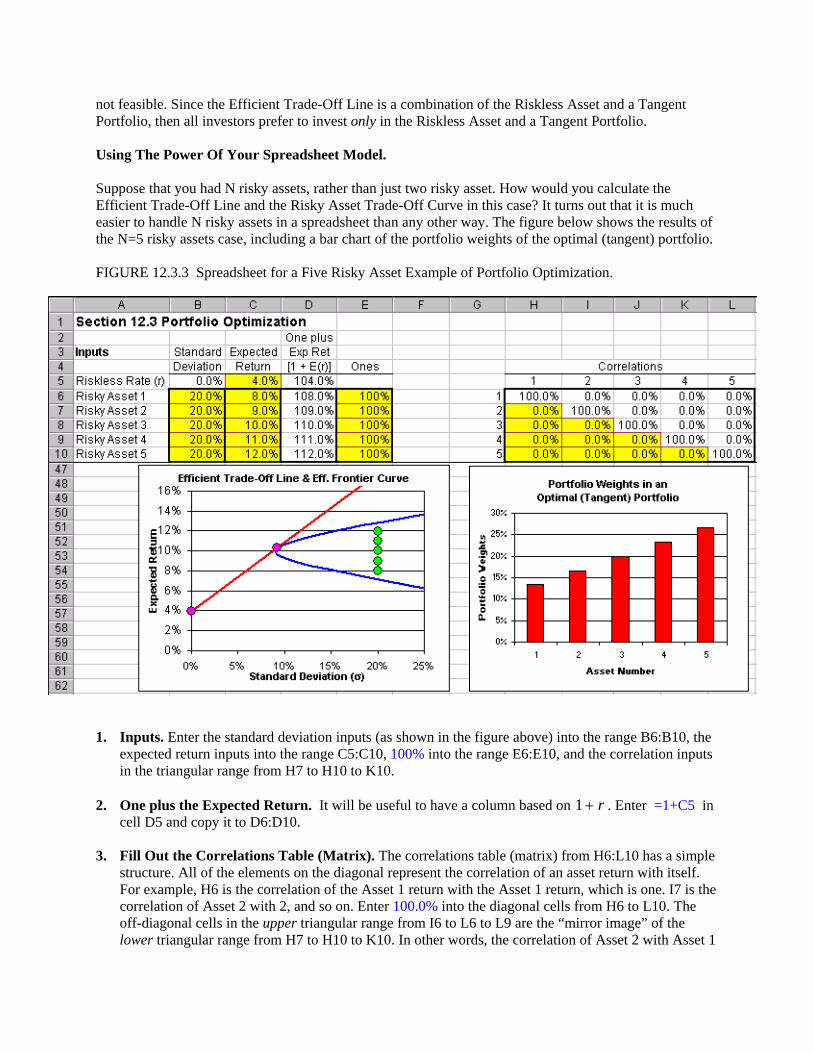
not feasible. Since the Efficient Trade-Off Line is a combination of the Riskless Asset and a Tangent Portfolio, then all investors prefer to invest only in the Riskless Asset and a Tangent Portfolio. Using The Power Of Your Spreadsheet Model. Suppose that you had N risky assets, rather than just two risky asset. How would you calculate the Efficient Trade-Off Line and the Risky Asset Trade-Off Curve in this case? It turns out that it is much easier to handle N risky assets in a spreadsheet than any other way. The figure below shows the results of the N=5 risky assets case, including a bar chart of the portfolio weights of the optimal (tangent) portfolio. FIGURE 12.3.3 Spreadsheet for a Five Risky Asset Example of Portfolio Optimization.

Inputs. Enter the standard deviation inputs (as shown in the figure above) into the range B6:B10, the expected return inputs into the range C5:C10, 10

1. 0% into the range E6:E10, and the correlation inputs

ular range from H7 to H10 to K10.

2. . It will be useful to have a column based on

in the triang

One plus the Expected Return r+1 . Enter =1+C5 in cell D5 and copy it to D6:D10.

3.

he

Fill Out the Correlations Table (Matrix). The correlations table (matrix) from H6:L10 has a simple structure. All of the elements on the diagonal represent the correlation of an asset return with itself. For example, H6 is the correlation of the Asset 1 return with the Asset 1 return, which is one. I7 is tcorrelation of Asset 2 with 2, and so on. Enter 100.0% into the diagonal cells from H6 to L10. Theoff-diagonal cells in the upper triangular range from I6 to L6 to L9 are the “mirror image” of the lower triangular range from H7 to H10 to K10. In other words, the correlation of Asset 2 with Asset 1

in I6 is equal to the correlation of Asset 1 with Asset 2 in H7. Enter =H7 in cell I6, =H8 in J6, =I8 in J7, etc. Each cell of the upper triangular range from I6 to L6 to L9 should be set equal to its mirror image cell in the lower triangular range from H7 to H10 to K10.

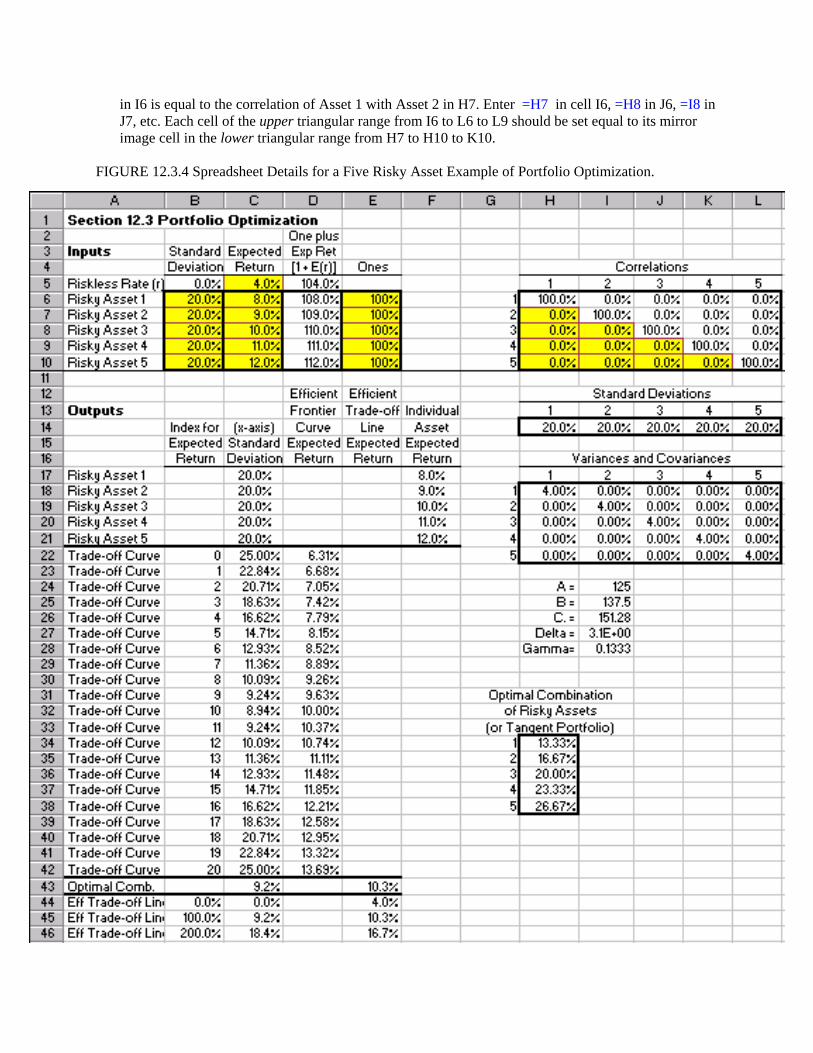
FIGURE 12.3.4 Spreadsheet Details for a Five Risky Asset Example of Portfolio Optimization.

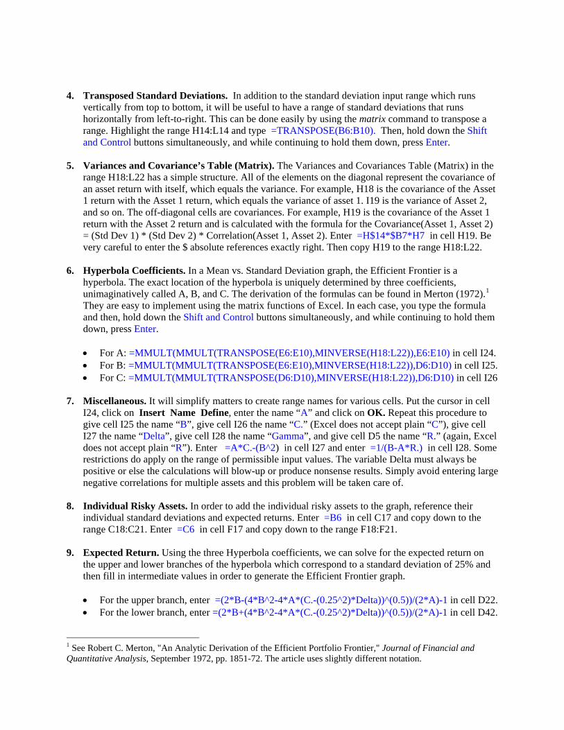
Transposed Standard Deviations. In addition to the standard deviation input range which runs vertically from top to bottom, it will be useful to have a range of standard deviations that runs horizontally from left-to-right. This can be done easily by using the matrix command to tran

4.

spose a range. Highlight the range H14:L14 and type =TRANSPOSE(B6:B10). Then, hold down the Shift

5.

f

) = (Std Dev 1) * (Std Dev 2) * Correlation(Asset 1, Asset 2). Enter =H$14*$B7*H7 in cell H19. Be

L22. 6.

plement using the matrix functions of Excel. In each case, you type the formula and then, hold down the Shift and Control buttons simultaneously, and while continuing to hold them

• For B: =MMULT(MMULT(TRANSPOSE(E6:E10),MINVERSE(H18:L22)),D6:D10) in cell I25.

7.

cel

must always be positive or else the calculations will blow-up or produce nonsense results. Simply avoid entering large

8. h, reference their

individual standard deviations and expected returns. Enter =B6 in cell C17 and copy down to the

9.

the upper and lower branches of the hyperbola which correspond to a standard deviation of 25% and

•

and Control buttons simultaneously, and while continuing to hold them down, press Enter.

Variances and Covariance’s Table (Matrix). The Variances and Covariances Table (Matrix) in the range H18:L22 has a simple structure. All of the elements on the diagonal represent the covariance oan asset return with itself, which equals the variance. For example, H18 is the covariance of the Asset 1 return with the Asset 1 return, which equals the variance of asset 1. I19 is the variance of Asset 2, and so on. The off-diagonal cells are covariances. For example, H19 is the covariance of the Asset 1 return with the Asset 2 return and is calculated with the formula for the Covariance(Asset 1, Asset 2

very careful to enter the $ absolute references exactly right. Then copy H19 to the range H18:

Hyperbola Coefficients. In a Mean vs. Standard Deviation graph, the Efficient Frontier is a hyperbola. The exact location of the hyperbola is uniquely determined by three coefficients, unimaginatively called A, B, and C. The derivation of the formulas can be found in Merton (1972).1 They are easy to im

down, press Enter.

• For A: =MMULT(MMULT(TRANSPOSE(E6:E10),MINVERSE(H18:L22)),E6:E10) in cell I24.

• For C: =MMULT(MMULT(TRANSPOSE(D6:D10),MINVERSE(H18:L22)),D6:D10) in cell I26

Miscellaneous. It will simplify matters to create range names for various cells. Put the cursor in cellI24, click on Insert Name Define, enter the name “A” and click on OK. Repeat this procedure to give cell I25 the name “B”, give cell I26 the name “C.” (Excel does not accept plain “C”), give cell I27 the name “Delta”, give cell I28 the name “Gamma”, and give cell D5 the name “R.” (again, Exdoes not accept plain “R”). Enter =A*C.-(B^2) in cell I27 and enter =1/(B-A*R.) in cell I28. Some restrictions do apply on the range of permissible input values. The variable Delta

negative correlations for multiple assets and this problem will be taken care of.

Individual Risky Assets. In order to add the individual risky assets to the grap

range C18:C21. Enter =C6 in cell F17 and copy down to the range F18:F21.

Expected Return. Using the three Hyperbola coefficients, we can solve for the expected return on

then fill in intermediate values in order to generate the Efficient Frontier graph.

• For the upper branch, enter =(2*B-(4*B^2-4*A*(C.-(0.25^2)*Delta))^(0.5))/(2*A)-1 in cell D22. For the lower branch, enter =(2*B+(4*B^2-4*A*(C.-(0.25^2)*Delta))^(0.5))/(2*A)-1 in cell D42.

1 See Robert C. Merton, "An Analytic Derivation of the Efficient Portfolio Frontier," Journal of Financial and Quantitative Analysis, September 1972, pp. 1851-72. The article uses slightly different notation.

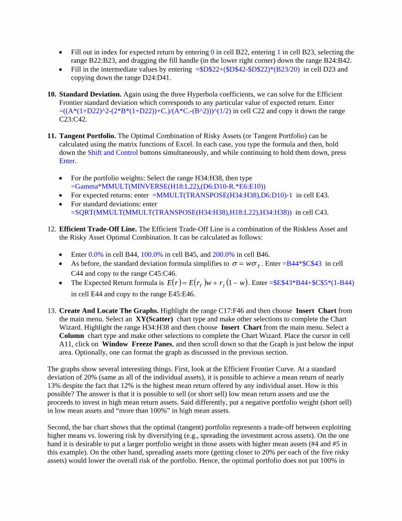
• Fill out in index for expected return by entering 0 in cell B22, entering 1 in cell B23, selecting thrange B22:B23, and dragging the fil

e l handle (in the lower right corner) down the range B24:B42.

• Fill in the intermediate values by entering =$D$22+($D$42-$D$22)*(B23/20) in cell D23 and

10.

ndard deviation which corresponds to any particular value of expected return. Enter =((A*(1+D22)^2-(2*B*(1+D22))+C.)/(A*C.-(B^2)))^(1/2) in cell C22 and copy it down the range

11.

ted using the matrix functions of Excel. In each case, you type the formula and then, hold down the Shift and Control buttons simultaneously, and while continuing to hold them down, press

E(H18:L22),(D6:D10-R.*E6:E10)) • • For standard deviations: enter

2. Efficient Trade-Off Line. The Efficient Trade-Off Line is a combination of the Riskless Asset and

• l B45, and 200.0% in cell B46.

formula simplifies to

copying down the range D24:D41.

Standard Deviation. Again using the three Hyperbola coefficients, we can solve for the Efficient Frontier sta

C23:C42.

Tangent Portfolio. The Optimal Combination of Risky Assets (or Tangent Portfolio) can be calcula

Enter.

• For the portfolio weights: Select the range H34:H38, then type =Gamma*MMULT(MINVERSFor expected returns: enter =MMULT(TRANSPOSE(H34:H38),D6:D10)-1 in cell E43.

=SQRT(MMULT(MMULT(TRANSPOSE(H34:H38),H18:L22),H34:H38)) in cell C43.

1the Risky Asset Optimal Combination. It can be calculated as follows:

Enter 0.0% in cell B44, 100.0% in celσ = σ• As before, the standard deviation w

•

T . Enter =B44*$C$43 in cell C44 and copy to the range C45:C46. The Expected Return formula is ( ) ( ) ( )wrwrErE fT −+= 1 . Enter =$E$43*B44+$C$5*(1-B44)

13.

ce the cursor in cell A11, click on Window Freeze Panes, and then scroll down so that the Graph is just below the input

arly

w mean return assets and use the roceeds to invest in high mean return assets. Said differently, put a negative portfolio weight (short sell)

isky rall risk of the portfolio. Hence, the optimal portfolio does not put 100% in

in cell E44 and copy to the range E45:E46.

Create And Locate The Graphs. Highlight the range C17:F46 and then choose Insert Chart from the main menu. Select an XY(Scatter) chart type and make other selections to complete the Chart Wizard. Highlight the range H34:H38 and then choose Insert Chart from the main menu. Select a Column chart type and make other selections to complete the Chart Wizard. Pla

area. Optionally, one can format the graph as discussed in the previous section. The graphs show several interesting things. First, look at the Efficient Frontier Curve. At a standard deviation of 20% (same as all of the individual assets), it is possible to achieve a mean return of ne13% despite the fact that 12% is the highest mean return offered by any individual asset. How is this possible? The answer is that it is possible to sell (or short sell) lopin low mean assets and “more than 100%” in high mean assets. Second, the bar chart shows that the optimal (tangent) portfolio represents a trade-off between exploitinghigher means vs. lowering risk by diversifying (e.g., spreading the investment across assets). On the one hand it is desirable to put a larger portfolio weight in those assets with higher mean assets (#4 and #5 in this example). On the other hand, spreading assets more (getting closer to 20% per each of the five rassets) would lower the ove

the high mean assets, nor does it put 20% in each asset, but instead finds the best trade-off possible between theses two goals. Third, you should be delighted to find any mispriced assets, because these are delightful investment opportunities for you. Indeed, many investors spend money to collect information (do security analysis) which identifies mispriced assets. The bar chart shows you how to optimally exploit any mispriced assets

at you find. Below is a list of experiments that you might wish to perform. Notice as you perform these experim e, but still makes the fundame ng.

ly generate a negative weight (short sell)? iced due to a low standard deviation?

• What happens when the riskless rate is lowered?

means, standard deviations, and correlations. If an individual investor believes that an articular asset is mispriced, then this belief should be optimally exploited. Only under the special

uld the tangent portfolio also be the market ortfolio.

Here are so

•

o ermine the optimal portfolio. If you have monthly data,

r at

thents that the optimal portfolio exploits mispriced assets to the appropriate degre

ntal trade-off between gaining higher means vs. lowering risk by diversifyi

• What happens when an individual asset is underpriced (high mean return)? • What happens when an individual asset is overpriced (low mean return)? • Is it possible for a very low mean return to optimal• What happens when an individual asset is mispr• What happens when an individual asset is mispriced due to a high standard deviation?

• What happens when the riskless rate is raised? • What happens when risky assets 1 and 2 have a 99% correlation?

Fourth, in general terms the optimal (tangent) portfolio is not the same as the market portfolio. Eachindividual investor should determine his or her own tangent portfolio based on his or her own beliefs about assetpconditions and the restrictive assumptions of CAPM theory wop

me additional projects / enhancements you can do:

Obtain historical data for different asset classes (and/or assets in different countries) and calculate the means, standard deviations, and correlations. Then, forecast future means, standard deviations, and correlations using the historical data as your starting point, but making appropriate adjustments. Input those means, standard deviations, and correlations intthe spreadsheet model in order to detyou can switch from annual returns to monthly returns by simply entering the appropriate monthly returns numbers and then rescaling the graph appropriately (see how to format thegraph scale in the previous section).

• Make the spreadsheet model interactive by adding “spinners” (see the Black-Scholes model for an example of how to do this) or by downloading the interactive portfolio optimizewww.kelley.iu.edu/finweb/holden.htm Expand the number of risky assets to any number that you want. For example, expanding to six risky assets simply involves adding a sixth: (1) standard deviation in cell B11, (2) expected return in cell C11, (3) one plus expected return in cell D11, (4) 100% in cell(5) row of correlations in the range H11:M11 and column in the range M6:M10, (6) row of variances / covariances in the range H23:M23 and column in the range M18:M22. Finally,

•

E11,

reenter all of the matrix functions changing their references to the expanded ranges. Specifically, reenter matrix functions for: transposed standard deviations, A, B, C, tangent portfolio weights, tangent portfolio expected return, and tangent portfolio standard deviation.

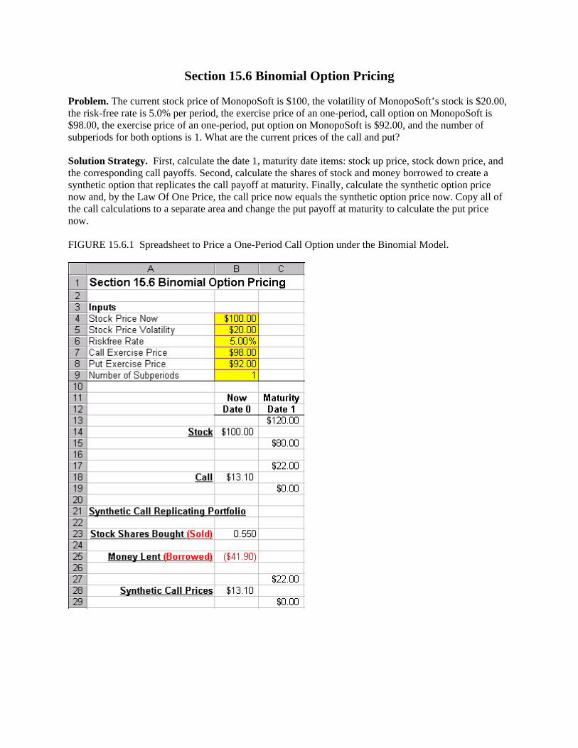
Section 15.6 Binomial Option Pricing Problem. The current stock price of MonopoSoft is $100, the volatility of MonopoSoft’s stock is $20.00, the risk-free rate is 5.0% per period, the exercise price of an one-period, call option on MonopoSoft is $98.00, the exercise price of an one-period, put option on MonopoSoft is $92.00, and the number of subperiods for both options is 1. What are the current prices of the call and put? Solution Strategy. First, calculate the date 1, maturity date items: stock up price, stock down price, and the corresponding call payoffs. Second, calculate the shares of stock and money borrowed to create a synthetic option that replicates the call payoff at maturity. Finally, calculate the synthetic option price now and, by the Law Of One Price, the call price now equals the synthetic option price now. Copy all of the call calculations to a separate area and change the put payoff at maturity to calculate the put price now. FIGURE 15.6.1 Spreadsheet to Price a One-Period Call Option under the Binomial Model.

How To Build Your Own Spreadsheet Model.

1. nd click on Window Freeze Panes. This freezes the top nine rows as an input

section at the top.

2. l

ock in the inputs, which will be useful for when we copy the formulas later on.

3. ns in $B$7 lock in the Call Exercise Price. Copy the Call

Payoff formula from cell C17 to cell C19.

4.

Inputs and Freeze Panes. Enter the inputs described above into the range B4:B9. Then, place the cursor in cell A10 a

Stock Prices. For the Date 0 Stock Price reference the Stock Price Now by entering =$B$4 in celB14. Calculate the Date 1 Stock Up Price = Stock Price Now + Stock Price Volatility / Number of Subperiods by entering =B14+$B$5/$B$9 in cell C13. Calculate the Date 1 Stock Down Price = Stock Price Now - Stock Price Volatility / Number of Subperiods by entering =B14-$B$5/$B$9 in cell C15. The $ signs in $B$4, $B$5, and $B$9 l

Call Payoffs. Calculate the Call Payoff = Max (Stock Price Now – Call Exercise Price, 0) by entering=MAX(C13-$B$7,0) in cell C17. The $ sig

Create A Synthetic Call Replicating Portfolio. For the Synthetic Call Replicating Portfolio, calculate the Stock Shares Bought (Sold) using the Hedge Ratio = (Call Up Payoff – Call Down Payoff) / (Stock Up Price – Stock Down Price). In cell B23, enter =(C17-C19)/(C13-C15). For theSynthetic Call Replicating Portfolio, calculate the amount of Money Lent (Borrowed) = (Call Up Payoff –Hedge Ratio * Stock Up Price) / (1 + Riskfree Rate / Number of Subperiods). In cell B25,enter =(C17-B23*C13)/(1+$B$6/$B$9). Notice that replicating a Call option requires Borrowing Money and Buying Shares of Stock. Specifically, Borrow $41.90 Dollars and Buy 0.550 Shares of Stock. The opposite pattern will be required to replicate a Put option.

5. ula = e /

$6/$B$9). Verify that the Synthetic Call’s payoff at maturity is equal to the Call’s payoff at maturity.

6.

cell B18. We see that the Binomial Option Pricing model predicts a one-period call price of $13.10.

(Optional) Synthetic Call Payoff. Check the Synthetic Call’s payoff at maturity using the formNumber of Shares of Stock * Stock Price at Maturity +Money Borrowed * (1 + Riskfree RatNumber of Subperiods). In cell C27, enter the payoff formula based on the Stock Up Price =B23*C13+B25*(1+$B$6/$B$9) and in cell C29, enter the payoff formula based on the Stock Down Price =B23*C15+B25*(1+$B

Calculate the Synthetic Option Price Now. The Synthetic Call Price can easily be calculated using the formula = Number of Shares of Stock * Stock Price Now + Money Borrowed. In cell B28, enter=B23*B14+B25. By the Law Of One Price, the Call Price Now is equal to the Synthetic Call Price Now. Enter =B28 in

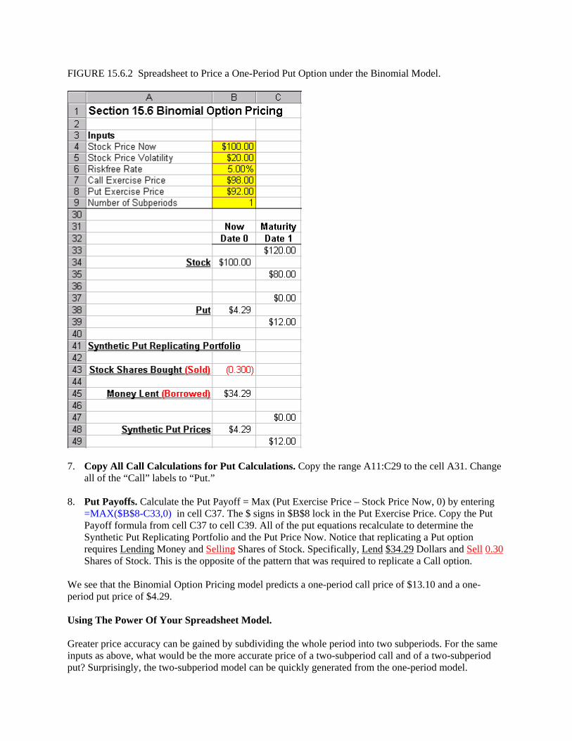
FIGURE 15.6.2 Spreadsheet to Price a One-Period Put Option under the Binomial Model.

7. Put Calculations. Copy the range A11:C29 to the cell A31. Change

8. Put

Copy All Call Calculations for all of the “Call” labels to “Put.”

Put Payoffs. Calculate the Put Payoff = Max (Put Exercise Price – Stock Price Now, 0) by entering =MAX($B$8-C33,0) in cell C37. The $ signs in $B$8 lock in the Put Exercise Price. Copy the Payoff formula from cell C37 to cell C39. All of the put equations recalculate to determine the Synthetic Put Replicating Portfolio and the Put Price Now. Notice that replicating a Put option requires Lending Money and Selling Shares of Stock. Specifically, Lend $34.29 Dollars and Sell 0.30

odel predicts a one-period call price of $13.10 and a one-

riod

put? Surprisingly, the two-subperiod model can be quickly generated from the one-period model.

Shares of Stock. This is the opposite of the pattern that was required to replicate a Call option. We see that the Binomial Option Pricing mperiod put price of $4.29. Using The Power Of Your Spreadsheet Model. Greater price accuracy can be gained by subdividing the whole period into two subperiods. For the sameinputs as above, what would be the more accurate price of a two-subperiod call and of a two-subpe

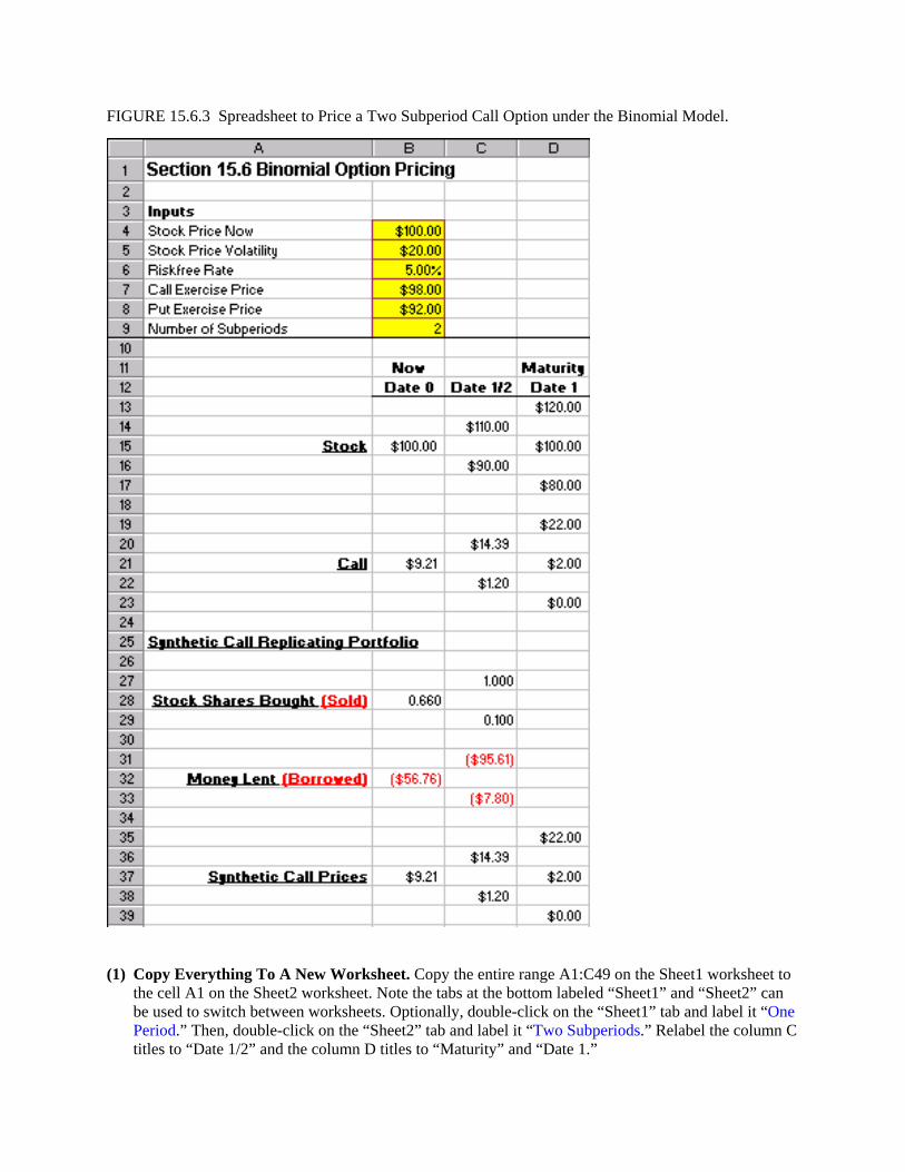
FIGURE 15.6.3 Spreadsheet to Price a Two Subperiod Call Option under the Binomial Model.

(1) Copy Everything To A New Worksheet. Copy the entire range A1:C49 on the Sheet1 worksheet to

the cell A1 on the Sheet2 worksheet. Note the tabs at the bottom labeled “Sheet1” and “Sheet2” can be used to switch between worksheets. Optionally, double-click on the “Sheet1” tab and label it “One Period.” Then, double-click on the “Sheet2” tab and label it “Two Subperiods.” Relabel the column C titles to “Date 1/2” and the column D titles to “Maturity” and “Date 1.”

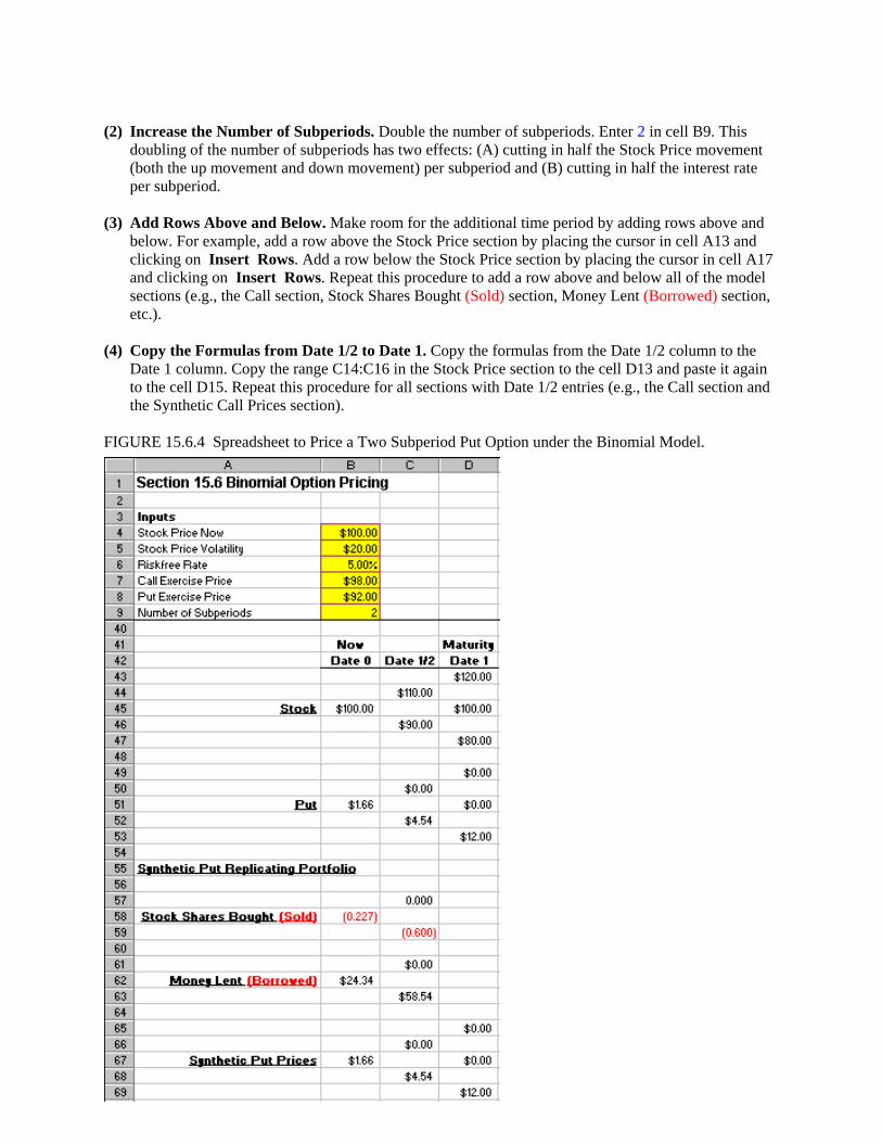
(2) Increase the Number of Subperiods. Double the number of subperiods. Enter 2 in cell B9. This

doubling of the number of subperiods has two effects: (A) cutting in half the Stock Price movement (both the up movement and down movement) per subperiod and (B) cutting in half the interest rate per subperiod.

(3) Add Rows Above and Below. Make room for the additional time period by adding rows above and

below. For example, add a row above the Stock Price section by placing the cursor in cell A13 and clicking on Insert Rows. Add a row below the Stock Price section by placing the cursor in cell A17 and clicking on Insert Rows. Repeat this procedure to add a row above and below all of the model sections (e.g., the Call section, Stock Shares Bought (Sold) section, Money Lent (Borrowed) section, etc.).

(4) Copy the Formulas from Date 1/2 to Date 1. Copy the formulas from the Date 1/2 column to the

Date 1 column. Copy the range C14:C16 in the Stock Price section to the cell D13 and paste it again to the cell D15. Repeat this procedure for all sections with Date 1/2 entries (e.g., the Call section and the Synthetic Call Prices section).

FIGURE 15.6.4 Spreadsheet to Price a Two Subperiod Put Option under the Binomial Model.

(5) Copy Selected Formulas from Date 0 to Date 1/2. Copy selected formulas from the Date 0 column

to the Date 1/2 columns. In the following order, copy the cell B28 to cell C27 and to cell C29, copy the cell B32 to the cell C31 and cell C33, copy the cell B37 to the cell C36 and to cell C38, and copy the cell B21 to the cell C20 and cell C22. Repeat this procedure for the Put sections.

As in the single period case, the Replicating Portfolio for the Call option requires Borrowing Money and Buying Shares of Stock, whereas the Replicating Portfolio for the Put option requires Lending Money and Selling Shares of Stock. Notice that the quantity of Money Borrowed or Lent and the quantity of Shares Bought or Sold changes over time and differs for up nodes vs. down nodes. This process of changing the replicating portfolio every period based on the realized up or down movement in the underlying stock price is called dynamic replication. The two-subperiod binomial model predicts a call price of $9.21 (vs. the one-period call price of $13.10) and predicts a put price of $1.66 (vs. the one-period put price of $4.29). The two-subperiod price is a more accurate representation of real-world options. The price accuracy can be increased further by subdividing the interval into further subperiods (4, 8, 16, 32, etc.). Typically, from 32 subperiods to 128 subperiods are required in order to achieve price accuracy to the penny. The procedure described above for doubling the one period model to a two subperiod model can be used to double the two subperiod model to a four subperiod model, double it again to an eight subperiod model, and so on up to an arbitrarily large number of subperiods.

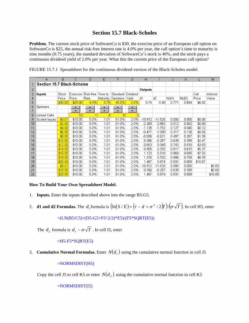
Section 15.7 Black-Scholes Problem. The current stock price of SoftwareCo is $30, the exercise price of an European call option on SoftwareCo is $25, the annual risk-free interest rate is 4.0% per year, the call option’s time to maturity is nine months (0.75 years), the standard deviation of SoftwareCo’s stock is 40%, and the stock pays a continuous dividend yield of 2.0% per year. What this the current price of the European call option? FIGURE 15.7.1 Spreadsheet for the continuous dividend version of the Black-Scholes model.

How To Build Your Own Spreadsheet Model. 1. Inputs. Enter the inputs described above into the range B5:G5. 2. d1 and d2 Formulas. The formula is d1 ( ) ( )( ) ( )TTdrES σσ /2//ln 2+−+ . In cell H5, enter =(LN(B5/C5)+(D5-G5+F5^2/2)*E5)/(F5*SQRT(E5)) The d formula is 2 Td σ−1 . In cell I5, enter =H5-F5*SQRT(E5) 3. Cumulative Normal Formulas. Enter ( )1dN using the cumulative normal function in cell J5 =NORMSDIST(H5) Copy the cell J5 to cell K5 or enter ( )2dN using the cumulative normal function in cell K5 =NORMSDIST(I5)

4. European Call Price Formula. The continuous dividend version of the Black-Scholes call formula is . In cell L5, enter ( ) ( ) rTdT EedNSedNC −− −= 21

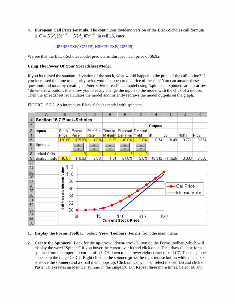
=J5*B5*EXP(-G5*E5)-K5*C5*EXP(-D5*E5) We see that the Black-Scholes model predicts an European call price of $6.92. Using The Power Of Your Spreadsheet Model. If you increased the standard deviation of the stock, what would happen to the price of the call option? If you increased the time to maturity, what would happen to the price of the call? You can answer these questions and more by creating an interactive spreadsheet model using “spinners.” Spinners are up-arrow / down-arrow buttons that allow you to easily change the inputs to the model with the click of a mouse. Then the spreadsheet recalculates the model and instantly redraws the model outputs on the graph. FIGURE 15.7.2 An interactive Black-Scholes model with spinners.

1. Display the Forms Toolbar. Select View Toolbars Forms from the main menu. 2. Create the Spinners. Look for the up-arrow / down-arrow button on the Forms toolbar (which will

display the word “Spinner” if you hover the cursor over it) and click on it. Then draw the box for a spinner from the upper left corner of cell C6 down to the lower right corner of cell C7. Then a spinner appears in the range C6:C7. Right click on the spinner (press the right mouse button while the cursor is above the spinner) and a small menu pops up. Click on Copy. Then select the cell D6 and click on Paste. This creates an identical spinner in the range D6:D7. Repeat three more times. Select E6 and

click on Paste. Select F6 and click on Paste. Select G6 and click on Paste. You now have five spinners in a row.

3. Create The Cell Links. Right click on the first spinner in the range C6:C7 and a small menu pops

up. Click on Format Control and a dialog box pops up. Enter the cell link “C8” in the Cell link edit box and click on OK. Repeat this procedure for the other four spinners. Link the spinner in D6:D7 to cell D8, link the spinner in E6:E7 to cell E8, etc. Click on the up-arrows and down-arrows of the spinners to see how they change the values in the linked cells.

4. Create Scaled Inputs. The values in the linked cells are always integers, but they can be scaled

appropriately to the problem at hand. In cell C9, enter =C8. In cell D9, enter =D8/20. In cell E9, enter =E8/4+0.01. In cell F9, enter =F8/10+0.01. In cell G9, enter =G8/100. Adding 0.01 to the standard deviation and time variables avoids having the formulas fail when those inputs equal zero.

5. Create Stock Price Inputs. In the range B9:B19, enter the values 0.01, 2, 4, 6, …, 20. In cell B20,

enter 0.01. In cell B21, enter =C9. In cell B22, enter 20. 6. Copy The Other Inputs. In cell C10, enter =C9. Copy the formula in cell C10 across and down the

range C10:G22. 7. Copy The Formulas. Select the fomulas in the range H5:L5 and copy them to the range H9:L22. 8. Add The Intrinsic Value. If the call option was maturing today, rather than later, the option payoff

would be equal to: Max (S - X, 0). This is the so-called “Intrinsic Value” of the call option. In cell M20, enter the formula

=MAX(B20-C20,0) Then copy this formula from the cell M20 to the range M21:M22. For convenience in graphing, select the range L20:L22 and press delete to eliminate the values in those cells. 9. Graph the Call Price and Intrinsic Value. Highlight the range B9:B22, then hold down the Control

button and (while still holding it down) select the range L9:M22. Next choose Insert Chart from the main menu. Select an XY(Scatter) chart type and make other selections to complete the Chart Wizard. Place the graph in the range B23:K36.

10. Freeze Panes. Put the cursor in cell A10 and select Window Freeze Panes from the main menu.

Move the cursor down to cell A36. This moves the graph into view. Your interactive spreadsheet model allows you to change Black-Scholes inputs and instantly see the impact on a graph of the call price and intrinsic value. This allows you to perform instant experiments on the Black-Scholes model. Below is a list of experiments that you might want to perform:

• What happens when the standard deviation is increased? • What happens when the time to maturity is increased? • What happens when the exercise price is increased? • What happens when the riskfree rate is increased? • What happens when the dividend yield is increased? • What happens when the standard deviation is really close to zero? • What happens when the time to maturity is really close to zero?

Notice that the Black-Scholes call price is usually greater than the payoff you would obtain if the call was maturing today (the “intrinsic value”). This extra value is called the “Time Value” of the option. Given your result in the last experiment above, can you explain why the extra value is called the “Time Value”?