Excel_Financial_Functions

CITCentre for Instructional Technology

Produced by

softwareseries

ExcelFinancial Functions I

CIT POLICY ON TECHNICAL SUPPORTThis guide has been produced to help you understand the basics about the database, software or resource in question. However, general technical support for these resources is NOT provided by CIT. It is hoped that this guide will help you understand the program enough to allow you to diagnose and troubleshoot whatever difficulty you are having. A targeted web search, the program/database Help file as well as fellow students are all excellent resources to aide you in this task. Do not underestimate the information available on the web to help solve your problem.

SUGGESTIONS, COMMENTS & REPORTING ERRORS If you have any suggestions/comments regarding future TechNotes, or if you would like to report an error, please feel free to contact us via email at the following address: [email protected]

TABLE OF CONTENTS

INTRODUCTION 1

TIME VALUE OF MONEY ‐ REVIEW 1

Simple Present & Future Value 1

Present & Future Value with Non‐Annual Compounding Periods 2

Effective and Nominal Rates 2

Present & Future Value with Continuous Compounding 3

Present & Future Value of an Annuity 3

An Annuity with Infinite Periods – A Perpetuity 4

Net Present Value and the Internal Rate of Return 4

Compound Annual Growth Rate 5

EXCEL FINANCIAL FUNCTIONS 6

PV, FV, RATE, NPER, PMT 6

EFFECT & NOMINAL 9

EXP 11

NPV, IRR & FVSCHEDULE 11

B A C K TO TA B LE OF C ON TEN TS

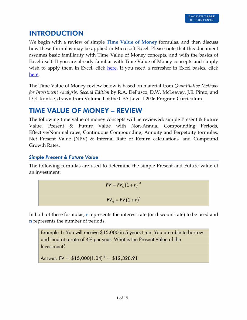
INTRODUCTION We begin with a review of simple Time Value of Money formulas, and then discuss how these formulas may be applied in Microsoft Excel. Please note that this document assumes basic familiarity with Time Value of Money concepts, and with the basics of Excel itself. If you are already familiar with Time Value of Money concepts and simply wish to apply them in Excel, click here. If you need a refresher in Excel basics, click here.

The Time Value of Money review below is based on material from Quantitative Methods for Investment Analysis, Second Edition by R.A. DeFusco, D.W. McLeavey, J.E. Pinto, and D.E. Runkle, drawn from Volume I of the CFA Level I 2006 Program Curriculum.

TIME VALUE OF MONEY – REVIEW The following time value of money concepts will be reviewed: simple Present & Future Value, Present & Future Value with Non‐Annual Compounding Periods, Effective/Nominal rates, Continuous Compounding, Annuity and Perpetuity formulas, Net Present Value (NPV) & Internal Rate of Return calculations, and Compound Growth Rates.

Simple Present & Future Value

The following formulas are used to determine the simple Present and Future value of an investment:

( ) nNPV FV r −= +1

( )nNFV PV r= +1

In both of these formulas, r represents the interest rate (or discount rate) to be used and n represents the number of periods.

Example 1: You will receive $15,000 in 5 years time. You are able to borrow and lend at a rate of 4% per year. What is the Present Value of the Investment?

Answer: PV = $15,000(1.04)-5 = $12,328.91

1 of 15

http://office.microsoft.com/training/training.aspx?AssetID=RC012005461033


Present & Future Value with Non-Annual Compounding Periods

In many Time Value of Money applications, the act of compounding occurs more frequently than on an annual basis. The following formulas modify the simple Present & Future value formulas to correct for more frequent compounding periods:

( )s mnrN mPV FV

−= +1

( )s mnrN mFV PV= +1

where m is equal to the number of compounding periods per year, rs is the stated annual rate, or nominal rate in Excel terminology (as will be discussed in the next section), and n now stands for the number of years. As such, mn represents the total number of compounding periods.

Example 2: You will receive $15,000 in 5 years time. You are able to borrow and lend at an annual rate of 4%, compounded monthly. What is the Present Value of the Investment?

Answer: PV = $15,000(1+(0.04/12))-60 = $12,285.05

Note that the simple Present & Future Value formulas in the previous section are a special case of these formulas where m is equal to 1.

Effective and Nominal Rates

As an extension of the previous formula, when a “stated” or “nominal” annual rate is quoted with non‐annual compounding periods, the following formula can be used to determine the effective annual rate:

Effective Rate = ( )msrm

+ −1 1

where, again, m is equal to the number of compounding periods per year, and rs is the nominal rate.

Example 3: You are charged an annual interest rate of 8.75% on your personal line of credit with your bank, compounded daily. What is the effective annual interest rate?

Answer: (1+(0.0875/365))365-1 = 0.0914, or 9.14%.

2 of 15


Present & Future Value with Continuous Compounding

While the above formulas deal with discrete compounding intervals, a number of applications in Finance deal with continuous compounding, when an infinite number of compounding periods are present. This convention is especially prominent in Option pricing models.

( )sr nNPV FV e−=

( )sr nNFV PV e=

where e is a mathematical constant equal to the base of the natural logarithm (≈2.718281828). The formula is calculated on a yearly basis.

Example 4: You have $12,280.96 in your bank account. You are able to invest the full amount for 5 years, continuously compounded at a rate of 4%. What is the Future Value of the investment?

Answer: FV = $12,280.96(e0.2) = $15,000

Present & Future Value of an Annuity

While the above formulas are used to calculate the fair value of a lump sum investment, separate formulas exist to calculate the Present & Future Value of an equal series of cash flows, referred to as Annuities. These formulas are shown below:

( )+−⎡ ⎤

⎢ ⎥=⎢ ⎥⎣ ⎦

nrPV Ar

11

1

( )⎡ ⎤+ −= ⎢ ⎥

⎢ ⎥⎣ ⎦

n

N

rFV A

r1 1

where A is the cash flow per period, r is the interest rate per period, and n is the number of periods.

Example 5: You are offered the option of choosing between an immediate, one-time, lump sum payment of $12,000, and $1,500 per year for 10 years. You are able to borrow and lend at an annual rate of 4%. Which option should you choose?

3 of 15


Answer: PV = $1,500[(0.3244)/0.04] = $1,500(8.1108) = $12,166.34. Therefore, you should choose the annuity because it is worth about $166 more in today’s dollars than the lump sum payment.

Keep in mind that these formulas assume the same cash flow per period. If the amount of the cash flow changes over time but is stable within intervals (i.e., $1,500 for years 1‐5, $2,000 for years 6‐10, etc.), an annuity calculation can be performed for each interval at the beginning of the interval, and then discounted back to present value. Otherwise, if the cash flows vary from period to period, using the Net Present Value (NPV) method will be necessary, as discussed below.

An Annuity with Infinite Periods – A Perpetuity

When the number of periods in the Present Value version of the annuity formula approaches infinity, the annuity formula reduces to a much simpler version:

APV

r=

In effect, a perpetual stream of cash flows, a perpetuity, can be valued simply by dividing the periodic cash flow by the periodic interest rate. A variant of this formula, the growing perpetuity (the denominator becomes r‐g, where g is the growth rate), is often an essential element in estimating the terminal value of an investment when conducting Discounted Cash Flow Analysis.

Net Present Value and the Internal Rate of Return

As mentioned above, the Net Present Value (NPV) method is used to properly discount a series of unequal cash flows back to present value. The NPV formula is as follows:

( )N

tt

t

CFNPV

r=

=+

∑0 1

where CFt equals the relevant cash flow at time t, and r is equal to the discount rate. The rate obtained by setting NPV to 0 and solving for r is referred to as the Internal Rate of Return.

4 of 15


Compound Annual Growth Rate

The last formula to be reviewed deals with calculating a compound annual growth rate for an investment or accounting value.

Rearranging the simple Future Value formula to solve for r, we obtain the following:

N

NFVr

PV⎛ ⎞= −⎜ ⎟⎝ ⎠

1

1

In many cases, you may see the interest rate above labelled as g (for growth rate) or CAGR (for Compound Annual Growth Rate). This is because the formula is often applied to situations where the variable cannot be correctly viewed as an interest rate. For example, change in accounting values (such as Total Assets, Sales, etc.) are often measured with this formula.

Example 6: Company ABC Inc. had $150 and $175 million in Total Assets as at December 31st, 2001 and 2006 respectively. Calculate the Compound Annual Growth Rate in total assets over the 5 year period.

Answer: CAGR = (175/150)0.2 -1 = 0.0313 or 3.13%.

5 of 15


EXCEL FINANCIAL FUNCTIONS

Please note that this section will make references to the solved examples on pages 1‐5 above.

PV, FV, RATE, NPER, PMT

When calculating Present and Future value using a computing aide (spreadsheet program or a financial calculator), there are always five variables involved in the calculation: the present value, future value, interest rate, number of periods, and the periodic payment (or annuity). One can solve for any of these variables if the other four are provided, and in Excel, a function exists for calculating each. The five functions are: PV, FV, RATE, NPER and PMT.

With the exception of the continuous compounding formula, these functions will work for any of the Present and Future value formulas that we’ve discussed above, including annuities.

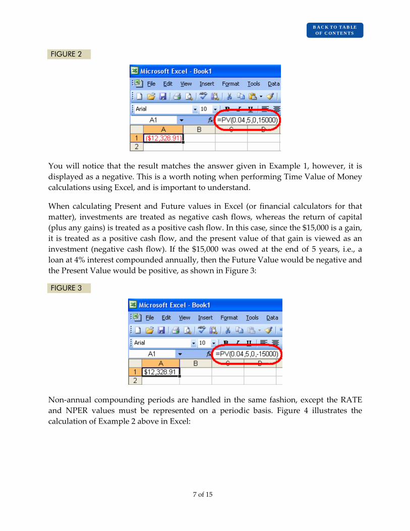
As an example, Figure 1 illustrates the syntax for the PV function:

FIGURE 1

Typing in the beginning of the function prompts the entry of the four remaining variables plus the [type] option which can be specified to indicate whether payments are made at the beginning (1) or the end of the period (0). If you omit a value for [type], Excel assumes that payments are made at the end of the period. When calculating simple Present and Future values, no value for payment exists. To indicate this, enter a value of zero for PMT.

Recalling Example 1 above, RATE = 0.04, NPER = 5, PMT = 0, and FV = 15000. Applying this example with Excel’s PV function is illustrated in Figure 2 below:

6 of 15


FIGURE 2

You will notice that the result matches the answer given in Example 1, however, it is displayed as a negative. This is a worth noting when performing Time Value of Money calculations using Excel, and is important to understand.

When calculating Present and Future values in Excel (or financial calculators for that matter), investments are treated as negative cash flows, whereas the return of capital (plus any gains) is treated as a positive cash flow. In this case, since the $15,000 is a gain, it is treated as a positive cash flow, and the present value of that gain is viewed as an investment (negative cash flow). If the $15,000 was owed at the end of 5 years, i.e., a loan at 4% interest compounded annually, then the Future Value would be negative and the Present Value would be positive, as shown in Figure 3:

FIGURE 3

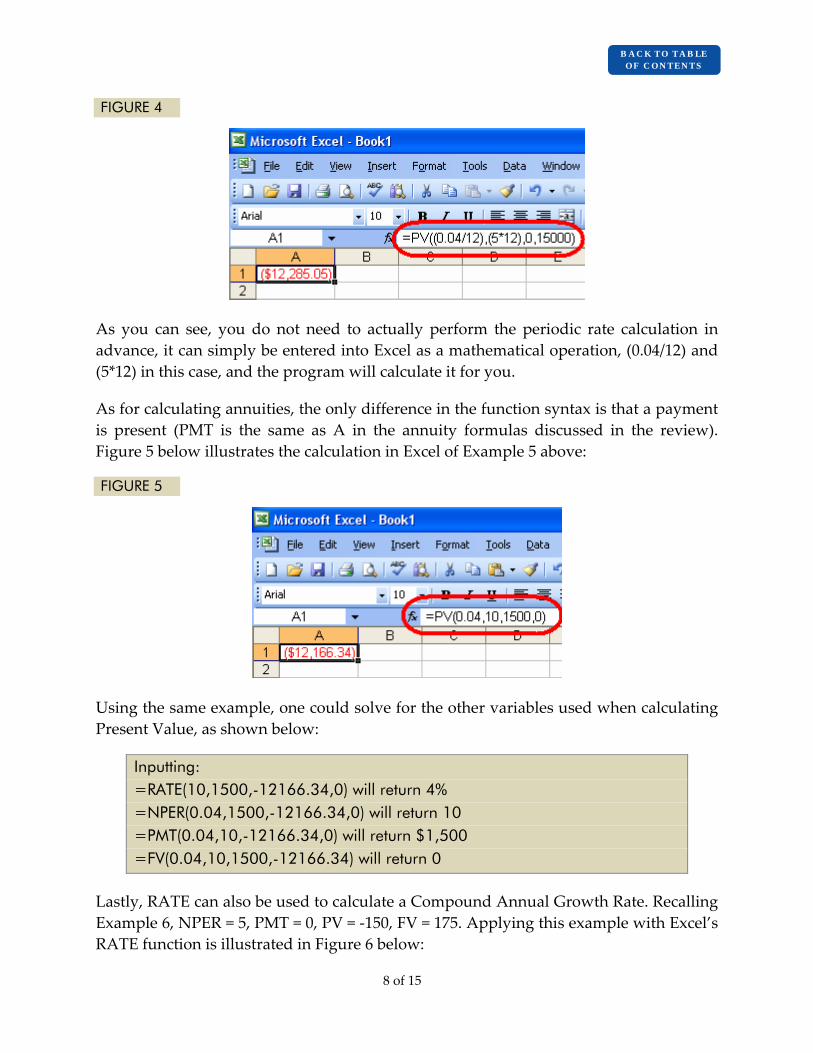
Non‐annual compounding periods are handled in the same fashion, except the RATE and NPER values must be represented on a periodic basis. Figure 4 illustrates the calculation of Example 2 above in Excel:

7 of 15


FIGURE 4

As you can see, you do not need to actually perform the periodic rate calculation in advance, it can simply be entered into Excel as a mathematical operation, (0.04/12) and (5*12) in this case, and the program will calculate it for you.

As for calculating annuities, the only difference in the function syntax is that a payment is present (PMT is the same as A in the annuity formulas discussed in the review). Figure 5 below illustrates the calculation in Excel of Example 5 above:

FIGURE 5

Using the same example, one could solve for the other variables used when calculating Present Value, as shown below:

Inputting: =RATE(10,1500,-12166.34,0) will return 4% =NPER(0.04,1500,-12166.34,0) will return 10 =PMT(0.04,10,-12166.34,0) will return $1,500 =FV(0.04,10,1500,-12166.34) will return 0

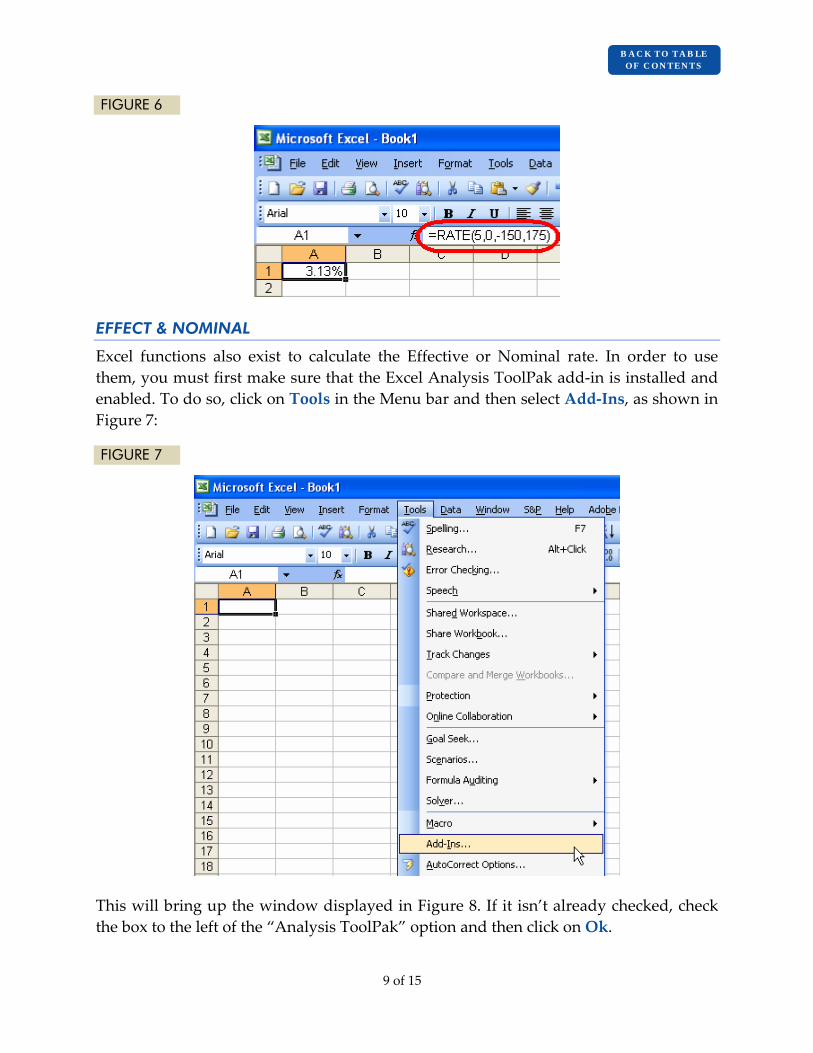
Lastly, RATE can also be used to calculate a Compound Annual Growth Rate. Recalling Example 6, NPER = 5, PMT = 0, PV = ‐150, FV = 175. Applying this example with Excel’s RATE function is illustrated in Figure 6 below:

8 of 15


FIGURE 6

EFFECT & NOMINAL

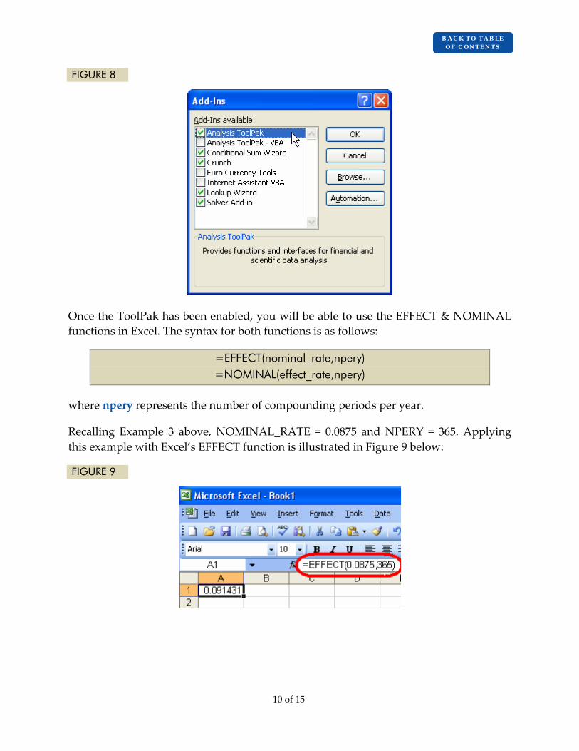
Excel functions also exist to calculate the Effective or Nominal rate. In order to use them, you must first make sure that the Excel Analysis ToolPak add‐in is installed and enabled. To do so, click on Tools in the Menu bar and then select Add‐Ins, as shown in Figure 7:

FIGURE 7

This will bring up the window displayed in Figure 8. If it isn’t already checked, check the box to the left of the “Analysis ToolPak” option and then click on Ok.

9 of 15


FIGURE 8

Once the ToolPak has been enabled, you will be able to use the EFFECT & NOMINAL functions in Excel. The syntax for both functions is as follows:

=EFFECT(nominal_rate,npery) =NOMINAL(effect_rate,npery)

where npery represents the number of compounding periods per year.

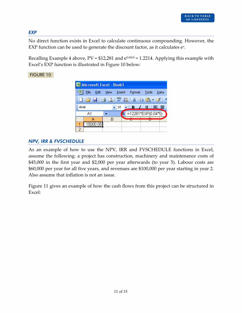
Recalling Example 3 above, NOMINAL_RATE = 0.0875 and NPERY = 365. Applying this example with Excel’s EFFECT function is illustrated in Figure 9 below:

FIGURE 9

10 of 15


EXP

No direct function exists in Excel to calculate continuous compounding. However, the EXP function can be used to generate the discount factor, as it calculates ex.

Recalling Example 4 above, PV = $12,281 and e0.04(5) = 1.2214. Applying this example with Excel’s EXP function is illustrated in Figure 10 below:

FIGURE 10

NPV, IRR & FVSCHEDULE

As an example of how to use the NPV, IRR and FVSCHEDULE functions in Excel, assume the following: a project has construction, machinery and maintenance costs of $45,000 in the first year and $2,000 per year afterwards (to year 5). Labour costs are $60,000 per year for all five years, and revenues are $100,000 per year starting in year 2. Also assume that inflation is not an issue.

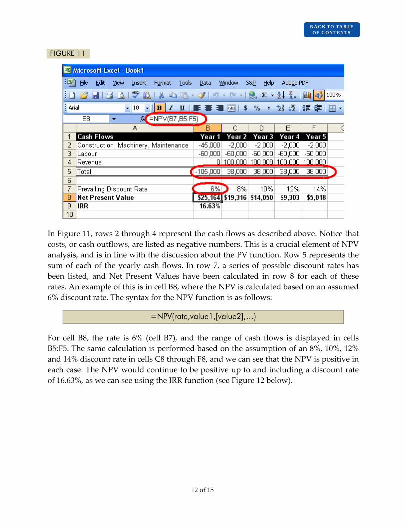
Figure 11 gives an example of how the cash flows from this project can be structured in Excel:

11 of 15


FIGURE 11

In Figure 11, rows 2 through 4 represent the cash flows as described above. Notice that costs, or cash outflows, are listed as negative numbers. This is a crucial element of NPV analysis, and is in line with the discussion about the PV function. Row 5 represents the sum of each of the yearly cash flows. In row 7, a series of possible discount rates has been listed, and Net Present Values have been calculated in row 8 for each of these rates. An example of this is in cell B8, where the NPV is calculated based on an assumed 6% discount rate. The syntax for the NPV function is as follows:

=NPV(rate,value1,[value2],…)

For cell B8, the rate is 6% (cell B7), and the range of cash flows is displayed in cells B5:F5. The same calculation is performed based on the assumption of an 8%, 10%, 12% and 14% discount rate in cells C8 through F8, and we can see that the NPV is positive in each case. The NPV would continue to be positive up to and including a discount rate of 16.63%, as we can see using the IRR function (see Figure 12 below).

12 of 15


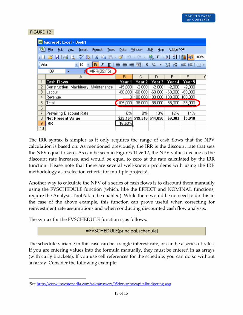
FIGURE 12

The IRR syntax is simpler as it only requires the range of cash flows that the NPV calculation is based on. As mentioned previously, the IRR is the discount rate that sets the NPV equal to zero. As can be seen in Figures 11 & 12, the NPV values decline as the discount rate increases, and would be equal to zero at the rate calculated by the IRR function. Please note that there are several well‐known problems with using the IRR methodology as a selection criteria for multiple projects1.

Another way to calculate the NPV of a series of cash flows is to discount them manually using the FVSCHEDULE function (which, like the EFFECT and NOMINAL functions, require the Analysis ToolPak to be enabled). While there would be no need to do this in the case of the above example, this function can prove useful when correcting for reinvestment rate assumptions and when conducting discounted cash flow analysis.

The syntax for the FVSCHEDULE function is as follows:

=FVSCHEDULE(principal,schedule)

The schedule variable in this case can be a single interest rate, or can be a series of rates. If you are entering values into the formula manually, they must be entered in as arrays (with curly brackets). If you use cell references for the schedule, you can do so without an array. Consider the following example:

1See http://www.investopedia.com/ask/answers/05/irrvsnpvcapitalbudgeting.asp

13 of 15

http://www.investopedia.com/ask/answers/05/irrvsnpvcapitalbudgeting.asp


Entering =FVSCHEDULE(5000,{0.05,0.06,0.07}) returns $5,954.55, which is the same as $5,000*(1.05)*(1.06)*(1.07)

Now assume that 0.05, 0.06 and 0.07 are entered as values in cells A1, B1 and C1 respectively. Entering =FVSCHEDULE(5000,A1:C1) also returns $5,954.55.

In terms of calculating NPV, we will use just one interest rate and employ the FVSCHEDULE function to calculate discount factors. An illustration of this is shown in Figure 13 below:

FIGURE 13

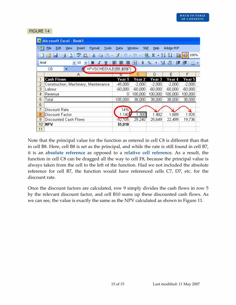
Here, the function has been used simply to calculate the first year discount factor, based on an assumed discount rate of 14%. Since a cell reference is used for the schedule, curly brackets are not required. Figure 14 shows how this can be extended for the remaining discount factors:

14 of 15


FIGURE 14

Note that the principal value for the function as entered in cell C8 is different than that in cell B8. Here, cell B8 is set as the principal, and while the rate is still found in cell B7, it is an absolute reference as opposed to a relative cell reference. As a result, the function in cell C8 can be dragged all the way to cell F8, because the principal value is always taken from the cell to the left of the function. Had we not included the absolute reference for cell B7, the function would have referenced cells C7, D7, etc. for the discount rate.

Once the discount factors are calculated, row 9 simply divides the cash flows in row 5 by the relevant discount factor, and cell B10 sums up these discounted cash flows. As we can see, the value is exactly the same as the NPV calculated as shown in Figure 11.

15 of 15 Last modified: 11 May 2007

Excel_Financial_Functions

Documents

Transcript of Excel_Financial_Functions