
Excel Level
76
7/14/2019 Excel Level http://slidepdf.com/reader/full/excel-level 1/76 207, Lok Center, Marol-Maroshi Road, Marol, Andheri (East), Mumbai 400 059. Tel: +91-22-2920 1583, 30910000 (100 lines). www.pragatisoftware.com Microsoft Excel 2007 Level 2 Version 164.04.02
-
Upload
tuku-singh -
Category
Documents
-
view
64 -
download
2
description
Knowledge about Excel
Transcript of Excel Level

7/14/2019 Excel Level
http://slidepdf.com/reader/full/excel-level 1/76
207, Lok Center, Marol-Maroshi Road, Marol, Andheri (East), Mumbai 400 059.
Tel: +91-22-2920 1583, 30910000 (100 lines). www.pragatisoftware.com
Microsoft Excel 2007 Level 2
Version 164.04.02

7/14/2019 Excel Level
http://slidepdf.com/reader/full/excel-level 2/76
Table of Contents
Chapter 1: Introduction to Microsoft Excel 2007 ................................................................. 1
About Excel............................................................................................................................... 1
Components of the Excel Window ........................................................................................... 1
Interacting with Excel ............................................................................................................... 2
Changing Default Settings ........................................................................................................ 3
Chapter 2: Cell References and Range Names ..................................................................... 4
Why Use Different Types of References? ................................................................................ 4
Types of Cell Reference: ........................................................................................................... 4
Named Ranges ......................................................................................................................... 7
Exercise .................................................................................................................................... 9
Chapter 3: Working with Formulas and Functions .............................................................. 10
Using Formulas in a Worksheet ............................................................................................. 10
Array Formulae....................................................................................................................... 10
Using functions ....................................................................................................................... 11
IF function .............................................................................................................................. 11
Nested IF ................................................................................................................................ 12
IF with AND ............................................................................................................................ 13
IF with OR ............................................................................................................................... 14
IF with NOT ............................................................................................................................. 14
Lookup Functions ................................................................................................................... 15
V-lookup ................................................................................................................................. 15
H-lookup ................................................................................................................................. 16
Making V-Lookup Dynamic .................................................................................................... 17
Index ....................................................................................................................................... 19
Index-Match ........................................................................................................................... 20
Exercise .................................................................................................................................. 21
Chapter 4: Data Validation ................................................................................................ 22
Setting Data Validation Rules ................................................................................................. 22
Methods of Data Validation ................................................................................................... 22
Exercise .................................................................................................................................. 24
Chapter 5:Protection ........................................................................................................ 25
Protecting a Worksheet by using Passwords ......................................................................... 25
Protecting a Workbook .......................................................................................................... 25
Protecting Part of a Worksheet.............................................................................................. 26
Password Protecting a File ..................................................................................................... 26
Case Study ....................................................................................................................... 28
Chapter 6: Sorting a Database ........................................................................................... 29

7/14/2019 Excel Level
http://slidepdf.com/reader/full/excel-level 3/76
Simple Sort ............................................................................................................................. 29
Multilevel Sort ........................................................................................................................ 29
Customized Sorting ................................................................................................................ 30
Chapter 7: Filtering a Database ......................................................................................... 31
Auto Filter............................................................................................................................... 31
Number, Text or Date Filters .................................................................................................. 31
Filtering a List using Advanced Filter ...................................................................................... 32
Filtering Unique Records ........................................................................................................ 33
Exercise .................................................................................................................................. 33
Chapter 8: Subtotals ......................................................................................................... 34
Display Subtotal at Single Level.............................................................................................. 34
Displaying Nested Subtotals ................................................................................................... 35
Chapter 9:Pivot Tables ...................................................................................................... 36
Examining Pivot Tables........................................................................................................... 36
Format a PivotTable report .................................................................................................... 37
Calculate the Percentage of the field ..................................................................................... 38
Top/ Bottom Report ............................................................................................................... 38
Group Items in a PivotTable ................................................................................................... 38
Create a Graph using Pivot Data ............................................................................................ 38
Chapter 10:Conditional formatting ................................................................................... 40
Conditional Formatting using Cell Values (Column Based Conditional Formatting) ............. 40
Conditional Formatting using Formula (Record Based Conditional Formatting) ................... 41
Database Case Study ........................................................................................................ 42
Chapter 11:What-if-Analysis Tools .................................................................................... 43
Goal Seek ................................................................................................................................ 43
Projecting Figures Using a Data Table .................................................................................... 44
What-If Scenarios ................................................................................................................... 45
Merge Scenarios from Another Worksheet ........................................................................... 47
Protecting Scenarios .............................................................................................................. 47
Chapter 12: Working with multiple worksheets, workbooks and applications .................... 49
Creating Links between Different Worksheets ...................................................................... 49
Creating links between different software ............................................................................ 50
Workgroup collaboration ....................................................................................................... 51
Merging workbooks ............................................................................................................... 52
Tracking changes .................................................................................................................... 52
Creating Hyper Link ................................................................................................................ 53
Chapter 13:-Working with Charts ...................................................................................... 55
Creating Charts using Chart Tools .......................................................................................... 55
Including Titles and Values in Charts using Chart Tools ......................................................... 56
Formatting charts ................................................................................................................... 57
Charts for my Data ................................................................................................................. 57
Chart Templates ..................................................................................................................... 57

7/14/2019 Excel Level
http://slidepdf.com/reader/full/excel-level 4/76
Exercise .................................................................................................................................. 58
Chapter 14:Macros ........................................................................................................... 59
Trust Center settings .............................................................................................................. 59
Creating a macro .................................................................................................................... 59
Recording a Macro ................................................................................................................. 60
Running a Macro Using Menu Commands............................................................................. 60
Writing a macro ...................................................................................................................... 61
Creating a sub procedure ....................................................................................................... 62
Creating a function ................................................................................................................. 63
Assigning a Macro to a Button ............................................................................................... 65
Final Assignment .................................................................................................................... 66
Shortcuts In Excel 2007 ..................................................................................................... 68
7/14/2019 Excel Level
http://slidepdf.com/reader/full/excel-level 5/76
1Pragati Software Pvt. Ltd.
Microsoft Excel 2007 Level 2.
Chapter 1: Introduction to Microsoft Excel 2007
Objective:
This chapter
Introduces you to the brand new layout of Microsoft Excel 2007.
Helps to Figure out how to change default settings.
Makes the user comfortable with the tool in general.
About Excel
Microsoft Excel is a powerful spreadsheet application from Microsoft Corporation. It makes it easy for
you to create various kinds of spreadsheets, tables and statements along with the graphical
representation of data. While working in Excel, you can make use of its most important feature of
automatic recalculation, to save time and effort.
In Excel, you work with worksheets, which consist of rows and columns that intersect to form cells.
Cells contain various kinds of data that you can format, sort, and analyze. You can also create charts
based on the data contained in cells. An Excel file is called a workbook, which by default contains
three worksheets.
Tips: Default number of sheets to open can be set to a maximum of 255.
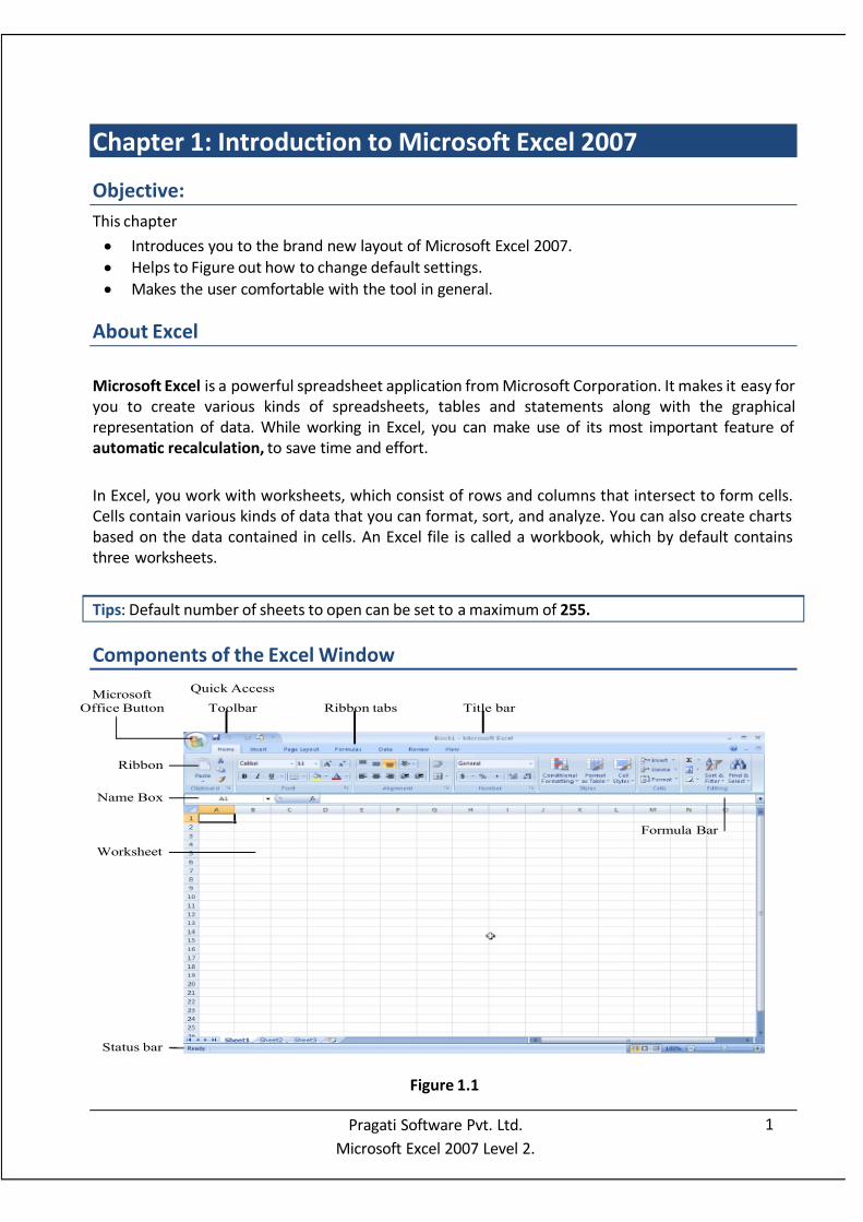
Components of the Excel Window
Quick Access
Toolbar
Ribbon
Title bar Ribbon tabs
Name Box
Worksheet
Status bar
Formula Bar
Microsoft
Office Button
Figure 1.1

7/14/2019 Excel Level
http://slidepdf.com/reader/full/excel-level 6/76
2Pragati Software Pvt. Ltd.
Microsoft Excel 2007 Level 2.
The components of the Excel window interact with the program or display information about what
you are working on. Some of these components are explained below:
Quick Access Toolbar: Displays commands for saving the current workbook, undoing the last action,
and repeating the last action. You can customize the Quick Access Toolbar by adding buttons for
frequently used commands. The Quick Access Toolbar can be moved below the Ribbon.
Ribbon: Each Ribbon tab activates a Ribbon, which in turn contains groups of commands or functions.
Within each group are buttons and commands.
Gallery: Galleries might display within a Ribbon but more often are drop-down groups of commands
or functions. They use icons or other graphics to show the results of commands rather than the
commands themselves.
Interacting with Excel
You interact with Excel by typing and by using the mouse to choose commands, make selections, click
buttons and options.
Using the Ribbon
The Ribbon is the main container for menus and tools. When you choose a Ribbon tab, the Ribbon
displays Ribbon groups that contain tools such as buttons and lists. Some of these tools expand to
display simple lists and some display galleries, as shown in Figure 1.2. A list is a collection of relatedcommands or selections.
Using galleries
A gallery is an interactive list of options. Each gallery displays the options under the clicked command.
For example, the font gallery shows the different font face options available. Some galleries use live
preview. When you move the pointer over options on a gallery, each option is previewed on whatever
Ribbon
group
Gallery
Figure 1.2

7/14/2019 Excel Level
http://slidepdf.com/reader/full/excel-level 7/76
3Pragati Software Pvt. Ltd.
Microsoft Excel 2007 Level 2.
Figure 1.3
is selected in the worksheet. For example, if you select text in the worksheet, and display the Font
gallery, moving the pointer over each font in the gallery causes the selected text on the screen to
display in that font.
Using Tools
When you point to a tool, a description called a super tooltip appears. The super tooltip provides lessdescription than Help, but more than an ordinary screen tip.
Tips: Press the “Alt” key to see the shortcuts to navigate through the ribbon.
Changing Default Settings
Excel allows you to change many aspects of its behavior and how you interact with it. You can change
default settings such as number of iterations, font, file locations, and the file that opens on starting
Excel.
To select the dialog box of Options you
need to click on MS-Office Button thenselect Excel Options.
The Personalize Option
You can change workbook settings by using
the Personalize Options to change the type
of font, size of the font, number of
worksheets in the workbook and can also
activate the Developer tab, which is used
for macros.
The Save Option
The Save Option allows you to change the
default file location, file format, and
AutoRecover settings of the file.

7/14/2019 Excel Level
http://slidepdf.com/reader/full/excel-level 8/76
4Pragati Software Pvt. Ltd.
Microsoft Excel 2007 Level 2.
Chapter 2: Cell References and Range Names
Objective:
After completing this chapter, you will be able to know
Meaning and usage of cell references. Type of cell references.
Usage of range names.
Why Use Different Types of References?
When we copy a reference from one cell to another, it gets updated automatically. Say, we have a
reference in cell C1 as A1 and we copy the same to D1, it automatically updates itself to B1.
Sometimes, we need to keep a part of the used cell references as constant. This can be done using
different types of cell references.
Types of Cell Reference:
There are three types of cell references as mentioned below;
1) Relative cell references
2) Absolute cell references
3) Mixed cell references
Relative Cell References
Relative references are the default cell references in Excel. When you copy and paste a relative cell
reference, it is updated automatically to suit the cell in which it is pasted. For Example,
If you want to calculate HRA as 50% of basic, you can write the formula =H2*50%
This is the HRA for one employee to apply this to all the records, you may drag the formula down till
the last record, as shown in Figure 2.2.
Figure 2.1
Figure 2.2

7/14/2019 Excel Level
http://slidepdf.com/reader/full/excel-level 9/76
5Pragati Software Pvt. Ltd.
Microsoft Excel 2007 Level 2.
Tips: Select the cells to fill and Press Ctrl + D to fill the range or double click on fill handle
Absolute Cell references
When you want to freeze a cell reference or you do not want a reference to change when you copy a
formula, you can use absolute cell references. To make a cell reference absolute, we place a dollar ($)
sign before the column name and row number of the reference.
Assume you want to calculate 10% of 1000, 2000, 3000, and 4000.
If you write as above, the formula when copied to the right would change itself to c1*b2, d1*c2etc.However, this is not the right calculation. We would need to freeze the cell reference A2, such that is
remains the same each time we copy the formula.
Here, A2 need to be changed to $A$2 to achieve the required output.
Tips: First select the cells from B2 to F2 and then press Ctrl+R keys. This would copy the formula from
B2 in C2, D2, E2 and F2.
Once this is done, we can see that, the formula when copied gives the required output as given in
Figure 2.5.
Mixed Cell References
However at times you may want to freeze only the row or column in a cell reference. In the below
example, we need to calculate 10%, 20%, 30%, 40% and 50% of 1000, 2000, 3000, 4000…… and so on.
Figure 2.3
Figure 2.4
Figure 2.5

7/14/2019 Excel Level
http://slidepdf.com/reader/full/excel-level 10/76
6Pragati Software Pvt. Ltd.
Microsoft Excel 2007 Level 2.
Figure 2.7
If you drag the formula towards the right it changes to c2*b3, d2*c3etc and once dragged down it
would change to b3*a4, b4*a5etc
However these are not the right formulae.
If we observe Figure 2.7 closely, we can see that, if we need to get the right answer, we would need
to freeze the row number of B2 (as it is common for all the formulae right and down) and the column
name for A3 (As it is common for all the formulae towards right and down). When copied, the
resultant formulae would be as given in Figure 2.8.
And the answer would be as given in Figure 2.9.This type of references where either the row or the
column number is frozen are called Mixed Cell References.
Figure 2.6
Figure 2.8

7/14/2019 Excel Level
http://slidepdf.com/reader/full/excel-level 11/76
7Pragati Software Pvt. Ltd.
Microsoft Excel 2007 Level 2.
Tips: Keep cursor near the cell reference and press f4 to toggle between the different cell references.
Press F4 key in cell reference
Named Ranges
Many a times, when we write formulas/functions, we need to select a range of cells. However, doing
this can be time consuming. Excel allows us to use a cell or a group of cells by its name. eg. Sum(Basic) sounds much easier compared to sum(H2:H101).However to do this, first we would need to name the
range H2:H10 as Basic.
Creating a Named Range
To name a range, we may use one of the following procedures
1) Select the range (eg: H2:H101) and type the name (eg: Sal) in the name box (see Figure 2.10).
2) If you want to name the cells with the value in one of the cells, you may select the range along with
the name, click on “Create from Selection” in the Formulas Tab, select one of the options and click
Ok.
3) You may also create a named range by clicking on “Define name” in Formulas Tab. Write the name
for the range in the name box , click on the refers to box, select the range you wish to name andclick Ok.
One Time $A$3
Second Time A$3
Third Time $A3
Fourth Time A3
Figure 2.9

7/14/2019 Excel Level
http://slidepdf.com/reader/full/excel-level 12/76
8Pragati Software Pvt. Ltd.
Microsoft Excel 2007 Level 2.
Now you may use the name instead of the range anywhere in the workbook. The usage of named
range can be seen in Figure 2.11.
Editing or Deleting Named Ranges
Sometimes we would need to rename or redefine a named range. This can be done from Formulas
Tab. In the "Formulas" Tab, click “Name Manager”. It gives a Name Manager Dialog box as shown in
Figure 2.12.
Figure 2.10
Figure 2.11
Figure 2.12

7/14/2019 Excel Level
http://slidepdf.com/reader/full/excel-level 13/76
9Pragati Software Pvt. Ltd.
Microsoft Excel 2007 Level 2.
To edit a named range, click on the Named Range that you want to edit and click on the Edit button.
An Edit Name dialog box as shown in Figure 2.13 appears where you may rename or redefine the
range name.
To delete a range, select the range from the Name Manager list and click Delete.
Tips: Press Ctrl + F3 to get a Name Manager dialog box
Exercise
1) Identify Relative, Absolute and Mixed references
a) A$1 b)$A$1
c) $A1 d) A1
2) In the Excel Training Folder, open Advanced Excel Assignment.xlsx file, go to Mixed-Cell sheet
calculate percentage sales of each product in different regions in such a way that when you copy the
cell formula of east sales and paste in each of the region columns, It automatically calculates sales
for the region.
Figure 2.13

7/14/2019 Excel Level
http://slidepdf.com/reader/full/excel-level 14/76
10Pragati Software Pvt. Ltd.
Microsoft Excel 2007 Level 2.
Chapter 3: Working with Formulas and Functions
Objectives
In this chapter we would learn
Effective usage of formulae and functions. If Functions.
Logical Functions.
Using Formulas in a Worksheet
Formulas are equations that perform calculations on values. A formula starts with an equal sign (=). It
contains at least two operands and at least one operation. For example, the following formula
multiplies 2 by 3 and adds 5 to the result.
=5+2*3
Operand in a formula can be functions, references or constants. Operators may be any arithmetic or
logical operator.
Note: Excel follows BODMAS rule to solve a formula when multiple operators are involved.
Array Formulae
Observe Figure 3.a. Here we have quantity and price of five products. We need to find the Total Sales
which is the result of adding together the product of quantity and price for all products. In a normal
scenario we would individually calculate the amount for each product and add them to get the
answer. However, to make things simpler we may also use Array Formulae.
Select B8 and write sum (A2:A6*B2:B6) and press Ctrl + Shift + Enter key combination to fill the
formula {=sum(A1:A3*B1:B3)} in the selected cell (Figure 3.2). This calculates quantity*price for all
the products in the cell B8.
Note: Curly Brackets ({}) around the formula indicates that it is applied to an array.
Figure 3.2Figure 3.1

7/14/2019 Excel Level
http://slidepdf.com/reader/full/excel-level 15/76
11Pragati Software Pvt. Ltd.
Microsoft Excel 2007 Level 2.
Using functions
Performing calculations on each value in a range of cells can be complicated and time-consuming.
Forexample, if you have a range consisting of 20 cells, a formula that adds each of these values will be
very long. Excel Functions simplify complex tasks. A
function is a predefined formula that performs a specific
calculation or other action on a number or a text string
and returns a value. You may specify the values on which
the function performs calculations.
The syntax of a function begins with the function name,
followed by an opening parenthesis, the arguments for
the function separated by commas and a closing
parenthesis. If the function starts a formula, type an
equal sign (=) before the function name. As you create a
formula that contains a function, the Formula Palette will
assist you.
Tips: From an empty cell, you may click on the fx symbol near the formula bar to see all the available
functions in excel.
The syntax of a function is as follows
=Function_name(argument1,argument2,….)
Example:
=SUM (A10, B5: B10, 50, 37)
You don’t need to memorize all the functions available and the arguments necessary for each
function. Instead, you can use Sigma sign (∑) which is used for sum or click on the drop down for some
more function like Max, Min, etc. Excel prompts you for required and optional arguments.
Tips: You can use "Alt + =" key combination to get the sum function on your worksheet.
IF function
In Chapter 2, we have seen how to calculate the income heads like HRA and DA. The formula we saw
was the same for the entire database. However, sometimes we need to decide the formula to apply in
a cell according to certain conditions. For example, incentives may be calculated according to thedepartment. This is where conditional functions like “IF” come in to the picture.
You can use the IF function to evaluate a condition. The IF function returns different values depending
on whether the condition is true or false. The syntax for the IF function is:
If(logical_test, [Value_if_true], [Value_if_false])
Figure 3.3

7/14/2019 Excel Level
http://slidepdf.com/reader/full/excel-level 16/76
12Pragati Software Pvt. Ltd.
Microsoft Excel 2007 Level 2.
The first argument is the condition that you want the function to evaluate. The second argument is
the value to be returned if the condition is true and the third argument is the value to be returned if
the condition is false. Second and third parameters are optional.
Example
Suppose you want to calculate HRA based on designation of the employees, if Designation is Managerthen HRA is1000 or else 500. Then the function code will be as follows:
=if (C2="Manager", 1000, 500)
As given in figure 3.3, above function calculates HRA as 1000 for Managers and 500 for others.
Nested IF
A Nested IF function is when a second IF function is placed inside the first in order to test additional
conditions.
The syntax for the Nested IF function is:
If(logical_test, [Value_if_true], If(logical_test, [Value_if_true], [Value_if_false]))
Examples:
You can use nested IF functions to evaluate complex conditions. For example, if the Salary <5000 then
tax is 5%, if salary between 5000 and 1000 then it is 10% else 15%.
=if(salary<5000,salary*.05,if(salary<10000,salary*.10,salary*.15))
Figure 3.5
Figure 3.4

7/14/2019 Excel Level
http://slidepdf.com/reader/full/excel-level 17/76
13Pragati Software Pvt. Ltd.
Microsoft Excel 2007 Level 2.
Suppose you want to assign letter grades to numbers referenced by the name Average Score. See the
following table.
If Average Score is Then returnGreater than 89 A
From 80 to 89 B
From 70 to 79 C
From 60 to 69 D
Less than 60 F
You can use the following nested IF function:
IF(AverageScore>89,"A",IF(AverageScore>79,"B",IF(AverageScore>69,"C",IF(AverageScore>59,"D","F")
)))
Tips:You can nest up to sixty four levels of If functions in a single formula.
IF with AND
AND is a logical function in excel which returns the combined truth value of two arguments or
conditions. It returns false only when all the conditions listed are false.
Syntax
AND(logical1, logical2...)
If there is a scenario where we have two conditions whose combined truth value would decide the
output of an IF function, we can use AND with IF.
Syntax using AND with If
If (and(Condition1, condition2….), True, False)
Example:
If we need to give 10% of his basic salary as incentive to every one working in “Sales” department“North” region, we would use the following formula.
=IF (AND (Department=”sales”, Region=”north”), 10%*Basic Salary, 0)

7/14/2019 Excel Level
http://slidepdf.com/reader/full/excel-level 18/76
14Pragati Software Pvt. Ltd.
Microsoft Excel 2007 Level 2.
IF with OR
OR is a logical function in excel which returns False if any one of the arguments returns false.
Syntax
OR(logical1, logical2...)
If there is a scenario where we have two conditions of which any one of the conditions is false, the if
should return the value in the false argument, we may use OR with IF.
Syntax using OR with If
If(OR(Condition1, condition2….), True, False)
Example:
If the employee is in Sales, Mktg or Hrd, then hra is 50% of Basic salary otherwise, it is 30% of Basic
salary.
if(or(Department ="Mktg",Department ="Sales",Department="Hrd"),Basic salary*.5,Basic salary*.3)
IF with NOT
Not is a logical function used to negate an argument.
Syntax
NOT(logical)
If we have a condition which when not satisfied we need to apply the formula, we may use NOT with
IF.
Syntax using NOT with If
If(NOT(Condition), True, False)
Example:
If we need to give an incentive to everyone but people working in the “Marketing” department we
may use the following formula.
IF(NOT(Department=”Mktg”),10%*salary,0)
Tips: There can be maximum 255 conditions which can be passed to AND/OR function and we can
pass only one condition to NOT.We may also use multiple not inside if.
Example
If you need to give an incentive to everyone but people from the sales ad admin department, you may
use the following function.

7/14/2019 Excel Level
http://slidepdf.com/reader/full/excel-level 19/76
15Pragati Software Pvt. Ltd.
Microsoft Excel 2007 Level 2.
If(and(not(department="Sales"),not(department="admin")),10%*salary,0)
Lookup Functions
Sometimes, we need to search for a value in a database based on a lookup value. For example, given
Employee Id, how can I look up the incentive value from some other sheet or some other file?
In such scenarios, depending on the source database, we may use one of the following lookupfunctions.
1) V-lookup (If the database is vertical as in Figure 3.6)
2) H-lookup (If the database is horizontal as in Figure 3.7)
V-lookup
If we need to the get the value of a column from some other file or sheet based on a common field,
you may use Vlookup. V-lookup is a function that searches for a value (lookup value) in the leftmost
column of a given database (table array)and returns a value in the same row from a column you
specify.
Syntax:
VLOOKUP(lookup_value,table_array,col_index_num,range_lookup)
You can write this function using Built-in Function Arguments dialog-box. Click on Formulas Tab and
search in the Lookup & Reference category for Vlookup. Click on Vlookup and you will get a Function
Arguments dialog box as shown in Figure 3.8.
Figure 3.6
Figure 3.7

7/14/2019 Excel Level
http://slidepdf.com/reader/full/excel-level 20/76
16Pragati Software Pvt. Ltd.
Microsoft Excel 2007 Level 2.
Figure 3.8
Lookup _value is the value to be found in the first column of the table. It is the value that you are
looking for. Lookup_value can be a value, a reference
or a text string.
Table_array is the table of information in which data
is looked up. It is the source database. Use a
reference to a range or a range name.Col_index_num is the column number in
table_array from which the matching value must be
returned.
Range_lookup is a logical value that specifies
whether you want VLOOKUP to find an exact match
or an approximate match. If Range Lookup is set as
FALSE or 0, VLOOKUP will find an exact match. If
exact match is not found, the error value #N/A is
returned. If it is set to TRUE or non-zero, it finds the
nearest value that is less than lookup value.
H-lookup
H-lookup function searches for a value in the top most row of a table, and then returns a value in the
same column from a row you specify.
Syntax:
HLOOKUP(lookup_value,table_array,row_index_num,range_lookup)
H-lookup works the same way as V-lookup. However, in this case we need to specify the row index
number instead of the column index number
Tips: You may also get the function argument box by the following methodType =vlookup( or =hlookup( as the case may be and press Ctrl+A.
Example of Vlookup with Range 0 (False):
Suppose you want to add incentive in the Salary Sheet according to the incentive table who's Range is
A1:B12 in the Incentive worksheet, do the following.
1) Select the cell, where you want the result.
2) Click on Insert Function –Select the Vlookup () function from Lookup and Reference category.
3) Lookup Value – Select A2 [The Employee code]
4) Table Array: Select the Incentive Sheet and Select the Range from $A$1:$B$12 [i.e. Employee
code and incentive Column]
5) Column Index: Type 2 [Column 2 is the Incentive column in Incentive table ]
6) Range Lookup: Type False [we are searching the exact match from the table for the lookup
value]
Tips: To remove #NA (Not Available Error), you can use the function Iferror. The Syntax of iferror is as
follows:

7/14/2019 Excel Level
http://slidepdf.com/reader/full/excel-level 21/76
17Pragati Software Pvt. Ltd.
Microsoft Excel 2007 Level 2.
Figure 3.9
=iferror(vlookup….),””)
Example of Vlookup with Range Non-Zero (True)
Suppose you want to add incentive based on salary Slab-wise. In this case, instead of If condition you
can use can use Vlookup with True range. In this scenario, we would create a table as given below. In
table array, select this table and in the field for range lookup, type “True” instead of “False”.
0 2%
5000 5%
10000 10%
15000 15%
Note: The table in this case would be sorted in ascending order of first column.
ExampleIn the "Advanced Excel Assignment" file, "emp_inf" sheet, we need to retrieve information of the
employee based on his employee id. To do this, we may use vlookup as follows.
To find the other details, you may use the same formula and change the column index number
accordingly.
Making V-Lookup Dynamic
When we have a dynamic database, where a new column gets added to the database frequently,
position of the current columns may also change. However, column index number of Vlookup doesnot update automatically with the growing database. This is where we would need to make VLookup
Dynamically pickup the column index number. To do this, we may use one of the following functions
to retrieve the column index number dynamically.
1) Column
2) Match

7/14/2019 Excel Level
http://slidepdf.com/reader/full/excel-level 22/76
18Pragati Software Pvt. Ltd.
Microsoft Excel 2007 Level 2.
Using Column Function in Vlookup
To make Vlookup dynamic, we may use the column header as an indicator that would dynamically
pickup the index number of the particular column in which the required value exist.
The syntax of using column function in vlookup
=vlookup(lookup_value,table_array,COLUMN(reference),Range_lookup)
Here, Reference parameter of column function would contain the cell reference of the column header
from the original database.
Example:
In the above example of vlookup, if we need to find the column index number dynamically we may
use column function as follows.
B1 is the reference to the column header of the First Name column in the 'Salary' worksheet.
Using Match Function in Vlookup
As we saw in the above case, we would require access to the original database or at least an idea as to
the current position of the column. However, this information would not always be available. Here we
would need to use a function that can retrieve the position of the column header just by the name.
A Match function does just the same. Match function returns the position of a string in a range.
Syntax of match function is as follows:
MATCH(lookup_value, lookup_array,[match_type])
Lookup_Value: It is the string that we are looking up for. It may be a string eg: "Salary" or a cell
reference where the string is stored.
Lookup_Array: It is the range from which we need to know the position of Lookup_value.
Match_Type: It is an optional parameter that is used to specify the type of match we require 0: Exact
match, 1: Less than, -1: Greater Than.
Figure 3.10

7/14/2019 Excel Level
http://slidepdf.com/reader/full/excel-level 23/76
19Pragati Software Pvt. Ltd.
Microsoft Excel 2007 Level 2.
For example, if we need to find out the position of the string "salary" in the first row of the salary
sheet, we would write,
=match("salary",salary!$1:$1,0)
We may use the match function instead of column Index number to get the column index number
dynamically.
The syntax of using match function in vlookup:
=vlookup(lookup_value,table_array,match(label,firstrow of source-database,0),Range_lookup)
Example:
In the emp_inf example, if we need to make the vlookup more dynamic using the column headers, we
may use match with vlookup as shown in figure 3.11. Here the match looks for the labels on each field
in the header of salary database and returns the position of the column dynamically.
Index
Sometimes, we would need to lookup for a data in the database based on its row number and column
number. Index function helps us do this.
Syntax of index function is as follows:
INDEX(array, row_number,[column_number])
As you can see there are two ways in which you can use the Index function. The first syntax is used to
look for data in a single database and the second syntax is used when more than one database isinvolved.
Example
Suppose we need to find the data at the intersection of row number 3 and column number 4 of a
database, we may use the following function.
=index(database,3,4)
Figure 3.j
Figure 3.11

7/14/2019 Excel Level
http://slidepdf.com/reader/full/excel-level 24/76
20Pragati Software Pvt. Ltd.
Microsoft Excel 2007 Level 2.
Index-Match
As discussed earlier, vlookup can look for the data based on the values in the first column of the
database. However, if we have a database where our lookup value is in the middle and we need to
search towards the left, we would have to move the column to the left most corner before we use
vlookup. Index function when used along with match helps us search for the data even if the lookup
value is not present on the left-most column.
The syntax for index-match is as follows:
INDEX(array,[MATCH(lookup_value,lookup_array,[match_type])],[Match(lookup_value,
lookup_array,[match_type])])
Here, you may use match function for row number or column number or both.
Example:
Suppose, from the data given in the below figure, we need to find the total sales, given year and
quarter, we may use the function.
=INDEX(database,MATCH(qtr 3,column header,0),MATCH(year,years column,0))
In the following figure, empcode is the third column. Here if we need to find out the DA or Salary
Based on the empcode, we normally copy and paste the column towards the left and use vlookup.Instead, we may use index match as given below.
Figure 3.12

7/14/2019 Excel Level
http://slidepdf.com/reader/full/excel-level 25/76
21Pragati Software Pvt. Ltd.
Microsoft Excel 2007 Level 2.
Exercise
1) Make a copy of the Salary worksheet from advanced excel assignment workbook. Calculate thefollowing incentive schemes
1) Incentive 1- Everyone working in “Sales” department gets 10% of their salary as incentive all
others gets 0
2) Incentive 2- Everyone working in “sales” or “marketing” department gets 5% of their salary as
incentive all others gets 2%.
3) Incentive 4- Give incentive as follows
Dept Incentive
CCD 1000
R&D 1500
Personnel 1200Others 800
2) Calculate the incentive scheme in Q.1 c using V-lookup
1) Make a column “Reporting Manager” after Salary column and deploy the employee code of the
managers to the employees according to their employee numbers as follows using V-Lookup.
Emp CodeReporting
Manager
1-35 14
36-55 61
56-75 16
75-100 5
Figure 3.13

7/14/2019 Excel Level
http://slidepdf.com/reader/full/excel-level 26/76
22Pragati Software Pvt. Ltd.
Microsoft Excel 2007 Level 2.
Chapter 4: Data Validation
Objective
This chapter
Helps you understand how to restrict data entry in a cell or a worksheet. Discusses the different Data Validation techniques in excel.
Suppose you do not want the user to enter a non text value in a cell or you want to restrict data entry
to certain values. You may use Data Validation for these.
Data Validation is a process which restricts the users from entering invalid data for individual cells or
cell ranges. It limits the data entry to a particular type, such as whole numbers, decimal numbers or
text and sets limit on valid entries.
Setting Data Validation Rules
To create a set of rules for data validation, do the following.
1) Select the cells for which you want to create a
validation rule.
2) On the Data tab, in the Data Tools group, click Data
Validation to open the Data Validation dialog box
(Figure 4.1).
3) Activate the Settings tab.
4) From the Allow list, select a data validation option.
5) From the Data list, select the operator you want.
Then complete the remaining entries.
6) Enter the Input Message if required in Input
Message tab.
7) Enter the error message if required in Error Alerttab.
8) Click OK to set the validation rule and close the dialog box.
Methods of Data Validation
Creating a List
A list is an effective form of data validation where the user is allowed to
select an option from a drop-down list which is built-in to the cell
(Figure 4.2). The data source may be written manually by the user or
selected from the same sheet.
Steps are as follows.
1) Select a blank cell
2) Select Data Tab
3) Select Data Validation from Data Tool group
4) Select List
5) In Source, select the cell with values, or type the data with comma.
Figure 4.1
Figure 4.2

7/14/2019 Excel Level
http://slidepdf.com/reader/full/excel-level 27/76
23Pragati Software Pvt. Ltd.
Microsoft Excel 2007 Level 2.
Tips: If the source is from a different sheet, create a named range for all the values and use the name
in the Source field for Data Validation.
Allow Numbers within Limits
1) In the Allow box, click Whole Number or Decimal.
2) In the Data box, select the type of restriction you want. For example, to set upper and lowerlimits, select Between.
3) Enter the minimum, maximum, or specific value to allow.
Allow Dates or Times within a Timeframe
1) In the Allow box, select Date or Time.
2) In the Data box, select the type of restriction you want. For example, to allow dates after a
certain day, select greater than.
3) Enter the start, end, or specific date or time to allow.
Allow Text of a Specified Length
1) In the Allow box, click Text Length.2) In the Data box, click the type of restriction you want. For example, to allow up to a certain
number of characters, click less than or equal to.
3) Enter the minimum, maximum, or specific length for the text.
Calculate What is Allowed Based on the Content of another Cell
1) In the Allow box, select the type of data you want.
2) In the Data box, select the operator (for the criteria) you want.
3) In the box or boxes below the Data box, click the cell that you want to use to specify what's
allowed. For example, to allow entries for an account only if the result won't go over the budget,
click Decimal for Allow, select less than or equal to for Data, and in the Maximum box, click the
cell that contains the budget amount.
Use a Formula to Calculate What is Allowed
1) In the Allow box, click Custom.
2) In the Formula box, enter a formula that calculates a logical value (TRUE for valid entries or
FALSE for invalid). For example, to give an incentive only if the dept is sales and the region west,
you may use the following custom formula =and(d2="sales",e2="west") .
To display an optional input message when the cell is clicked, click the Input Message tab, and make
sure that, the-Show Input Message When Cell is Selected - check-box is selected and fill in the title
and text for the message.
Specify how you want Microsoft Excel to respond when invalid data is entered:1) Click the Error Alert tab, and make sure the "Show Error Alert After Invalid Data is Entered"
check box is selected.
2) Select one of the following options for the Style box:
o To display an information message that does not prevent entry of invalid data, select
Information.

7/14/2019 Excel Level
http://slidepdf.com/reader/full/excel-level 28/76
24Pragati Software Pvt. Ltd.
Microsoft Excel 2007 Level 2.
o To display a warning message that does not prevent entry of invalid data, select
Warning.
o To prevent entry of invalid data, select Stop.
3) Fill in the title and text for the message (up to 225 characters).
If you do not enter a title or text, the title defaults to "Microsoft Excel" and the message to "Thevalue you entered is not valid. A user has restricted values that can be entered into this cell."
Exercise
1) Open Advance Excel Assignment workbook. In the sheet named Validation, so the following data
validations.
1) No duplicates should be allowed in emp_code..
2) Only text should be allowed in emp name.
3) Age should be only numeric data.
4) Salary should be between 5000 and 50000.
5) Joining Date should be less than current Date.
2) In the “emp_inf” sheet create a dropdown list of all the employee codes in cell B3.

7/14/2019 Excel Level
http://slidepdf.com/reader/full/excel-level 29/76
25Pragati Software Pvt. Ltd.
Microsoft Excel 2007 Level 2.
Chapter 5: Protection
Objectives:
After reading this chapter you will learn
How to prevent unauthorized changes to your worksheets How to password protect your workbooks
In the emp_inf example (Figure 5.1), if we wish to use the worksheet as a public template, we would
need to prevent un-authorized access to the
vlookup formulas. We would want to restrict the
data entry only to the cell B3. To do these, we
may use Protection.
In excel, there are 3 levels of Protection. Cell
Level, worksheet Level and Workbook level
Protection.
Protecting a Worksheet by using Passwords
To password-protect a worksheet,
1) Activate the Review ribbon tab.
2) In the Changes ribbon group, click Protect Sheet to open the
Protect Sheet dialog box.
3) Check the options you want.
4) Type a password and click OK. The Confirm Password dialog box
appears.
5) In the "Reenter Password to Proceed" box, type the same
password to confirm.
6) Click OK to close the password confirmation box and the dialog
box.
Protecting a Workbook
Workbook level protection can be done in two ways. Either you may wish to protect the workbook
structure (prevent changes like worksheets being moved,
deleted, inserted, hidden, unhidden, or renamed) or you may
want to protect the workbookwindow (ensure that a
workbook’s window is the same size and position each time it
is opened.)
To protect a workbook, follow the steps below.
1) Activate the Review ribbon tab.
2) In the Changes ribbon group, click Protect Workbook.
3) In the Protect Workbook dialog box that appears, select
either or both the options (Structure or Windows) as
Figure 5.2
Figure 5.3
Figure 5.1
Figure 5.3

7/14/2019 Excel Level
http://slidepdf.com/reader/full/excel-level 30/76
26Pragati Software Pvt. Ltd.
Microsoft Excel 2007 Level 2.
required.
4) To prevent others from removing workbook protection, you can set a password. After specifying
options in the Protect Workbook dialog box, click OK.
Protecting Part of a Worksheet
When you protect an entire worksheet, all the cells in the worksheet are locked by default. Thismeans that users cannot make changes to any cell in the worksheet. To allow the users to make
changes to particular cells only, you must unlock the cells manually before protecting the worksheet.
This will allow the users to change data only in the unlocked cells. You can hide the formula before
protecting the sheet, so that it is not visible to the user after sheet level protection is activated.
To password protect only part of a worksheet perform the following steps.
Step 1:
Select the range of cells that you want users to be able to modify.
Right-click and choose Format Cells to open the Format Cells dialog box.
Activate the Protection tab.
Clear the Locked check box, and click OK.
Follow Step 2 only if you wish to hide your formulae or proceed to step 3.
Step 2:
Select the range of cells with formulae that you want to hide from users.
Right-click and choose Format Cells to open the Format Cells dialog box.
Activate the Protection tab.
Check the "Hidden" check box along with the "locked" check box and click ok.
Follow step 4 to password protect the worksheet.
Step 3:
Activate the Review ribbon tab.
In the Changes ribbon group, click Protect Sheet to open the Protect Sheet dialog box,
Type a password and click OK. The Confirm Password dialog box appears.
In the "Re-enter password to proceed" box, type the same password.
Click OK to close both the password confirmation box and the dialog box.
Password Protecting a File
Alternatively, you may also wish to save your file with a password such that any user would be asked
for a password before he is able to view or modify your file. To do this, follow the steps below.1) Click on office-button > Save as
2) in the save as dialog box, click on tools > General options( Figure5.4).
3) Set the password to open or modify as the case may be.
4) Save the file.
Now the File is password protected.

7/14/2019 Excel Level
http://slidepdf.com/reader/full/excel-level 31/76
27Pragati Software Pvt. Ltd.
Microsoft Excel 2007 Level 2.
Note: To use an excel sheet as a template, save the file with .xlt extension.
Figure 5.4
7/14/2019 Excel Level
http://slidepdf.com/reader/full/excel-level 32/76
28Pragati Software Pvt. Ltd.
Microsoft Excel 2007 Level 2.
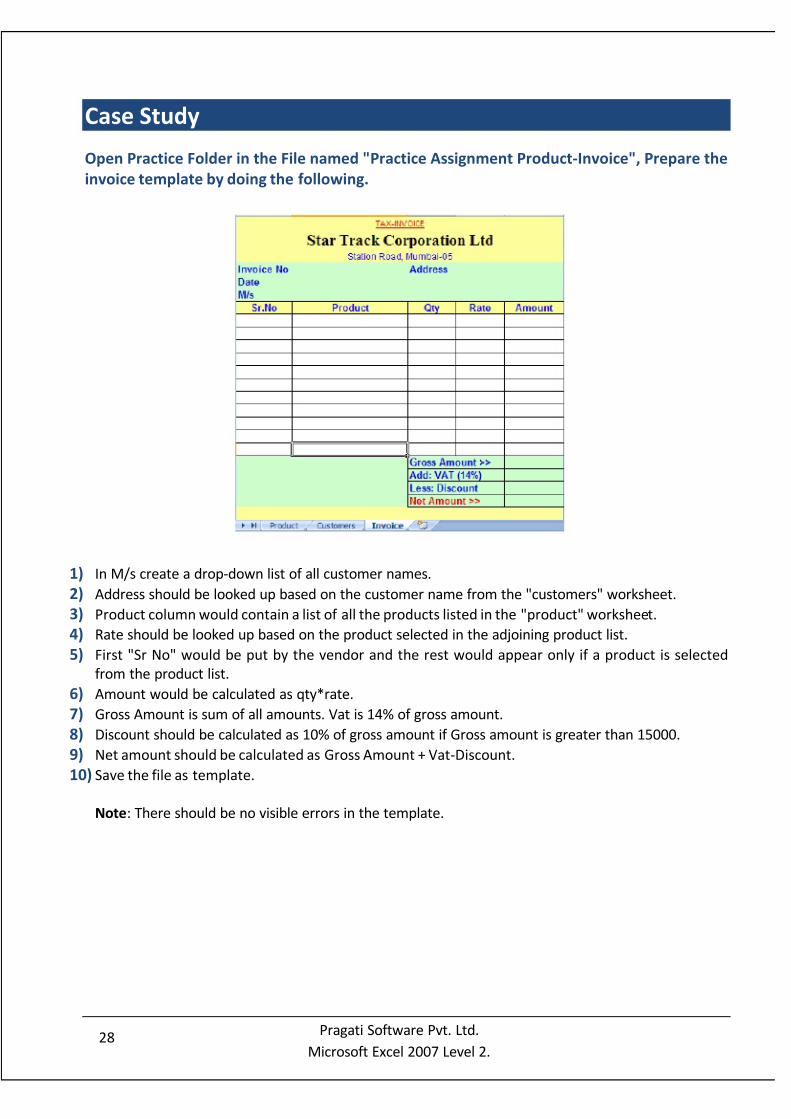
Case Study
Open Practice Folder in the File named "Practice Assignment Product-Invoice", Prepare the
invoice template by doing the following.
1) In M/s create a drop-down list of all customer names.
2) Address should be looked up based on the customer name from the "customers" worksheet.
3) Product column would contain a list of all the products listed in the "product" worksheet.
4) Rate should be looked up based on the product selected in the adjoining product list.
5) First "Sr No" would be put by the vendor and the rest would appear only if a product is selected
from the product list.
6) Amount would be calculated as qty*rate.
7) Gross Amount is sum of all amounts. Vat is 14% of gross amount.
8) Discount should be calculated as 10% of gross amount if Gross amount is greater than 15000.
9) Net amount should be calculated as Gross Amount + Vat-Discount.
10) Save the file as template.
Note: There should be no visible errors in the template.
7/14/2019 Excel Level
http://slidepdf.com/reader/full/excel-level 33/76
29Pragati Software Pvt. Ltd.
Microsoft Excel 2007 Level 2.
Figure 6.2
Chapter 6: Sorting a Database
Objectives
In this chapter you will learn
How to perform different types of sorting.
If you need to organize your data in a specific order based on a field, you may sort your data.
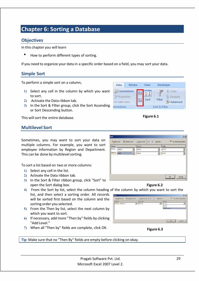
Simple Sort
To perform a simple sort on a column,
1) Select any cell in the column by which you want
to sort.
2) Activate the Data ribbon tab.
3) In the Sort & Filter group, click the Sort Ascending
or Sort Descending button.
This will sort the entire database.
Multilevel Sort
Sometimes, you may want to sort your data on
multiple columns. For example, you want to sort
employee information by Region and Department.
This can be done by multilevel sorting.
To sort a list based on two or more columns:
1) Select any cell in the list.
2) Activate the Data ribbon tab.
3) In the Sort & Filter ribbon group, click "Sort" to
open the Sort dialog box.
4) From the Sort by list, select the column heading of the column by which you want to sort the
list, and then select a sorting order. All records
will be sorted first based on the column and the
sorting order you selected.
5) From the Then by list, select the next column by
which you want to sort.
6) If necessary, add more "Then by" fields by clicking
"Add Level."
7) When all "Then by" fields are complete, click OK.
Tip: Make sure that no "Then By" fields are empty before clicking on okay.
Figure 6.1
Figure 6.3

7/14/2019 Excel Level
http://slidepdf.com/reader/full/excel-level 34/76
30Pragati Software Pvt. Ltd.
Microsoft Excel 2007 Level 2.
Customized Sorting
When we sort the data, region wise, it sorts either in the
ascending or descending order. However, if you want to sort
your data in a customized order, for Example East, West
North, and South, we would need to perform a custom sort.To perform a custom sort, follow the steps as under.
1) Select any cell in the list.
2) Activate the Data tab.
3) In the Sort & Filter group, click Sort to open the Sort
dialog box,
4) From the Sort By list, select the column heading of the
column by which you want to sort the list and from
sorting order, select Custom List
5) It will open the Custom List dialog box,
6) Type the sequence by which you wish to sort and click on "Add" button to add the list in custom
sort7) Click Ok
This will sort the data in the sequence you specified.
Figure 6.4

7/14/2019 Excel Level
http://slidepdf.com/reader/full/excel-level 35/76
31Pragati Software Pvt. Ltd.
Microsoft Excel 2007 Level 2.
Chapter 7: Filtering a Database
Objectives
This chapter teaches you
The different types of filter How to use them
At times, you will need to display only those rows of information that meet specific criteria. To help
you do this, you may use Filter.
Auto Filter
For commonly used criteria, Excel provides the AutoFilter
feature. Here’s how it works:
1) Select any cell in the list.
2) Activate the Data tab.
3) In the Sort & Filter group, click Filter to display the
AutoFilter arrows next to each column heading.
4) From the list for the column by which you want to filter,
select a criterion.
5) Click OK.
To clear the filter and show the entire list, click on filter again.
You can filter a list based on more complex criteria by using Excel’s Advanced Filtering features. For
example, you can display the records of all those employees whose salary is between 7000 and
12000. Excel provides two tools for specifying complex filter criteria:
1) Number, Text or date filters
2) Advanced Filter
Number, Text or Date Filters
Once you add a filter to data, you also get a Number, Text or Date Filter option in each fields
depending on the type of data in that column. These can be used for field specific filtering like "Begins
With", "Contains" for text fields, "Greater Than", "Lesser Than", "Between" for number fields or
"Before", "After" for date fields. Every filter field has a Custom Filter option where you may specify
formulas or options other than the ones that are already provided.
Figure 7.1
Fi ure 7.2 Fi ure 7.3 Fi ure 7.4

7/14/2019 Excel Level
http://slidepdf.com/reader/full/excel-level 36/76
32Pragati Software Pvt. Ltd.
Microsoft Excel 2007 Level 2.
From the drop-down list of the column for which you want to create criteria, choose Text Filters, Date
Filters or Number Filters, click on Custom to display the Custom AutoFilter dialog box.
1) Select the first comparison operator and its associated comparison criterion.
2) Select And or Or. By selecting "And", you’ll decrease the number of rows that meet the criteria.
By selecting "Or", you will increase the number of matching rows.
3)
Select the second comparison operator and its associated comparison criterion.4) Click OK.
Filtering a List using Advanced Filter
If you wish to filter your data such that only the records of employees of Sales and admin
departments from north and south region who earns between 7000-12000 or 15000-20000 are
displayed, auto filter will not serve the purpose. This is because one number filter cannot be applied
over another in Auto Filter. However, the above query requires us to do just the same on salary field.
So to solve this query, we may have to use Advanced-Filter.
While using Advanced Filter, we need to have a criteria range and a list range.
List range is your database. To create a criteria range, we need to make a copy of the column header
of the database.
1) Enter a comparison criterion below the cell that contains the
criteria label. You may use same row for "AND" criteria and
different rows for "OR" criteria. For example, the criteria given infigure 7.5 can be used to display only records of people in north
or south regions.
2) Activate the Data tab.
3) In the Sort & Filter group, click Advanced to open the Advanced
Filter dialog box. (Figure 7.6).
4) In the List Range box, select the cell range you want to filter. The
Criteria Range
List Range
Figure 7.5
Figure 7.6
7/14/2019 Excel Level
http://slidepdf.com/reader/full/excel-level 37/76
33Pragati Software Pvt. Ltd.
Microsoft Excel 2007 Level 2.
cell range must include the associated column headings.
5) In the Criteria Range box, select the cell range that contains your criteria.
6) Click OK.
Tip: While designing the criteria range, it is better to copy and paste the column header of the entire
database as the heading of the criteria range.
For better visibility, keep the criteria range and list range on different rows.
The Advanced Filter command filters your list in place, as Auto Filter does, but it does not display
drop-down lists for columns. Instead, you have to select the List Range i.e. your data, type criteria in a
criteria range on your worksheet and select the Criteria Range and in output range type the cell
address where you want to display the output. It is optional.
Filtering Unique Records
Advanced filter can also be used to filter out unique values in a list at a separate location. Though
remove duplicates functionality of excel can help in creating a list of unique values in a list, you would
need to copy paste the unique values, if you need it at a different location. To avoid this, use theadvance filter option as follows.
1) Select the column or click a cell in the range or list you want to filter.
2) On the Data Tab, Click Filter, and then click Advanced Filter.
3) Do one of the following.
o To filter the range or list in place, similar to using AutoFilter, click Filter the list, in-place.
o To copy the results of the filter to another location, click Copy to another location. Then,
in the Copy To box, enter a cell reference.
o To select a cell, click Collapse Dialog to temporarily hide the dialog box. Select the cell
on the worksheet, and then press Expand Dialog.
o Select the Unique records only check box.
Tips: Advanced filter, Copy to option copies on a same worksheet, if you want to copy the Filter datain to different worksheet, and then select the Advanced Filter command while you are at the
worksheet where you want the data to be placed.
Exercise
1) Open the sheet named Filter. Use Auto filter to display only records of
1) People working in sales or admin
2) People from North or South
2) Display records of people working in sales or admin, north or south whose salary is between 7000
and 12000.
3) Display records of people working in sales or admin, north or south whose salary is between 7000and 12000 or between 15000 and 20000.

7/14/2019 Excel Level
http://slidepdf.com/reader/full/excel-level 38/76
34Pragati Software Pvt. Ltd.
Microsoft Excel 2007 Level 2.
Chapter 8: Subtotals
Objectives:
After this chapter, you would be able to
Create single level summary of data using subtotals. Create multi level subtotals.
Many a times in our reporting, we need to do subtotals followed by Grand total at the end of report.
We generally add a row at the end of each group and use the SUM function to achieve this result.
Though there is nothing wrong in this method, the amount of manual intervention maximizes the
possibility of errors.
Excel provides an effective tool to solve this issue. Using the Subtotal functionality of excel, one can
automatically calculate subtotal and grand total values in a list.
Depending on the type of reporting we need to do, we may require to perform
1) Single Level Subtotal
2) Multi level Subtotal
Display Subtotal at Single Level
For performing Subtotal on data, first the table must be sorted on the field on which subtotal needs
to be done. For example, if you need to have region wise subtotal, we need to sort data on region. To
perform Subtotal,
1) Click on the Subtotals command from the Data Tab,
Outline Group.
2) A Subtotal dialog box appears as shown in figure 8.1.
3) Select the desired column from "At Each Change
In:"list box.
4) Select the function which you want to perform on
data from the "Use function" list box.
5) Select the column on which you want to perform
subtotals from the Add Subtotal To: field.
When you click the OK button, Microsoft Excel inserts a
subtotal row for each group of identical items in the
selected column.
There are a few more options in the Subtotal dialog as seen in figure 8.1. These are explained below.
Choosing a Summary Function
The first time you use the Subtotals command for a list, Microsoft Excel suggests a summary function
based on the type of data in the column you select in the Add Subtotal To box, Choose a different
calculation, such as Average, by selecting a different summary function in the Use Function box in the
Subtotal dialog box.
Figure 8.1

7/14/2019 Excel Level
http://slidepdf.com/reader/full/excel-level 39/76
35Pragati Software Pvt. Ltd.
Microsoft Excel 2007 Level 2.
Choosing the Values to Summarize
The first time you use the Subtotals command; the Add Subtotal To box displays the label of the right-
most column. You can leave that label as selected, or you can select the label of any other column in
the list. The next time you use the Subtotals command, Microsoft Excel displays the label of the last
column you selected.
Displaying Subtotal Rows above the Detailed Data
If you want your subtotal rows to appear above their associated detailed data and if you want the
Grand Total row to appear at the top of the list, clear the "Summary below Data" check box.
Displaying Nested Subtotals
Sometimes, you need to perform multiple levels of subtotals on data, for example you need to group
data on Region and then on Dept.
1) First, as discussed earlier, you need to sort the data on Region and then by Dept.
2) Click the Subtotals command from the Data Tab,
Outline Group.
3) Select the Region column from "At Each Change In"
list box.
4) Select the function which you want to perform on
data from the "Use function" list box.
5) Select the column on which you want to perform
subtotals from the Add Subtotal to field.
6) Click the OK button, to perform first level of subtotals
7) Again Select the Subtotal command and select the
Dept column from "At Each Change In" list box.
8) Select the function which you want to perform on
data from the "Use function" list box.
9) Select the column on which you want to performsubtotals from the "Add Subtotal to" field.
10) Clear the check box of "Replace the current subtotal"
before you clicks on the OK button.
Tips: If you want to copy only the summary details, select the outline where summary is present.
Select the columns required, press Alt; (to select only visible cells) then copy and paste it.
Figure 8.2

7/14/2019 Excel Level
http://slidepdf.com/reader/full/excel-level 40/76
36Pragati Software Pvt. Ltd.
Microsoft Excel 2007 Level 2.
Chapter 9:Pivot Tables
Objectives:
This chapter would help you learn how to
Create Pivot Tables. Make different reports using Pivot Tables.
Use advanced features of Pivot Tables.
A Pivot Table is an interactive worksheet based table that quickly summarizes large amounts of data
using the format and calculation methods you choose. It is called a Pivot Table because you can
rotate its row and column headings around the core data area to give you different views of the
source data. As source data changes, you can update a pivot table. It resides on a worksheet thus;
you can integrate a Pivot Table into a larger worksheet model using standard formulas. You can use a
PivotTable to analyze data in an Excel workbook or from an external database such as Microsoft
Access or SQL Server.
Examining PivotTables
The data on which a PivotTable is based is called the Source Data. Each column represents a field or
category of information, which you can assign to different parts of the PivotTable to determine how
the data is arranged. You can add four types of fields, as shown in figure 9.1. The fields are explained
in the following table:
Field Description
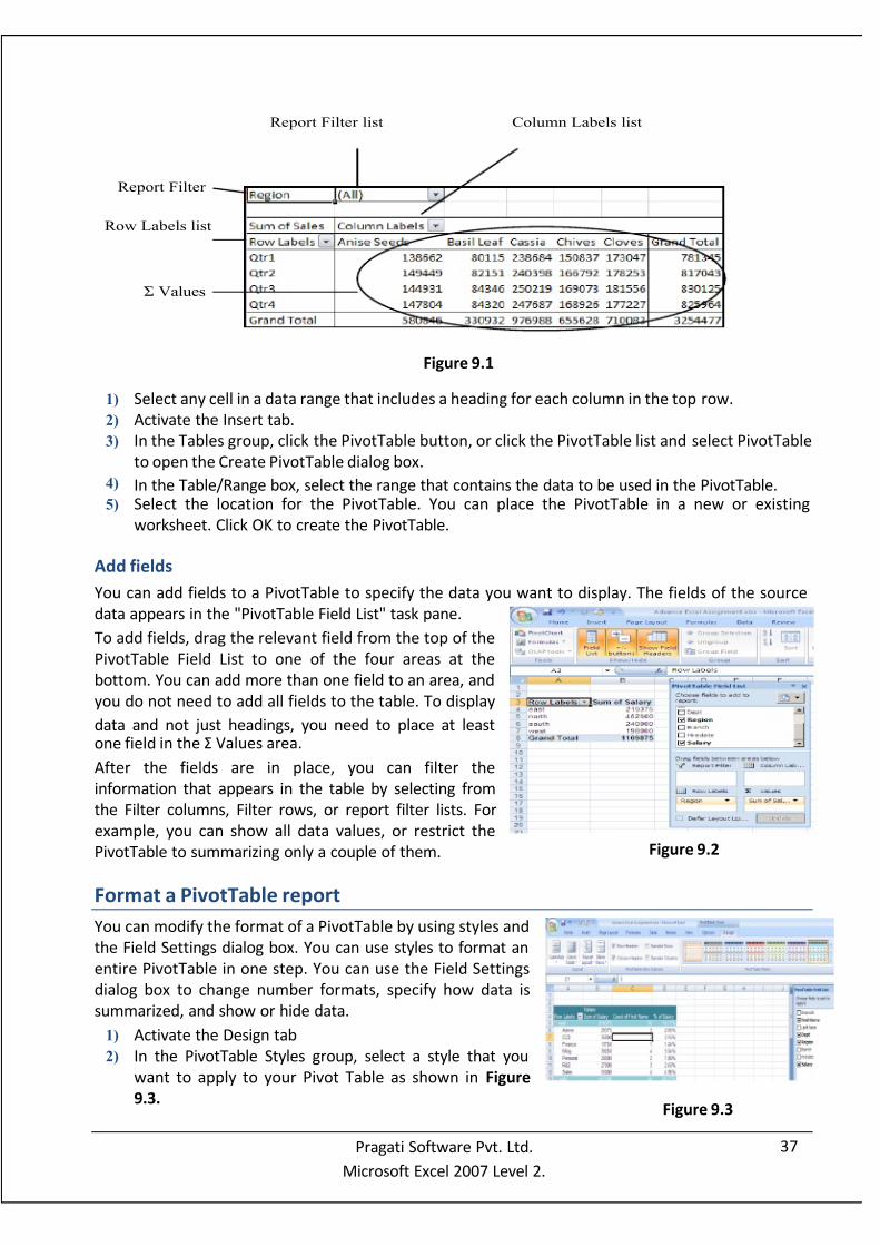
ReportFilter
Filters the summarized data in the PivotTable. If you select an item in
the report filter, the view of the PivotTable changes to display only the
summarized data associated with that item. For example, if Region is a
report filter, you can display the summarized data for North, West, or
all regions.
Row Labels
Displays the items in a field as row labels. For example given below, the
row labels are values in the Quarter field, which means that the table
shows one row for each quarter.
Column
Labels
Displays the items in a field as column labels. For example, given below,
the column labels are values in the Product field, which means that the
table shows one column for each product.
Σ Values
Contains the summarized data. These fields usually contain numeric
data, such as sales and inventory. The area where the data itself
appears is called the data area.
7/14/2019 Excel Level
http://slidepdf.com/reader/full/excel-level 41/76
37Pragati Software Pvt. Ltd.
Microsoft Excel 2007 Level 2.
Report Filter
Column Labels list
Σ Values
Row Labels list
Report Filter list
1) Select any cell in a data range that includes a heading for each column in the top row.
2) Activate the Insert tab.
3) In the Tables group, click the PivotTable button, or click the PivotTable list and select PivotTable
to open the Create PivotTable dialog box.
4) In the Table/Range box, select the range that contains the data to be used in the PivotTable.5) Select the location for the PivotTable. You can place the PivotTable in a new or existing
worksheet. Click OK to create the PivotTable.
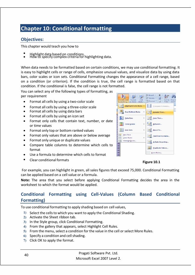
Add fields
You can add fields to a PivotTable to specify the data you want to display. The fields of the source
data appears in the "PivotTable Field List" task pane.
To add fields, drag the relevant field from the top of the
PivotTable Field List to one of the four areas at the
bottom. You can add more than one field to an area, and
you do not need to add all fields to the table. To display
data and not just headings, you need to place at leastone field in the Σ Values area.
After the fields are in place, you can filter the
information that appears in the table by selecting from
the Filter columns, Filter rows, or report filter lists. For
example, you can show all data values, or restrict the
PivotTable to summarizing only a couple of them.
Format a PivotTable report
You can modify the format of a PivotTable by using styles and
the Field Settings dialog box. You can use styles to format an
entire PivotTable in one step. You can use the Field Settings
dialog box to change number formats, specify how data is
summarized, and show or hide data.
1) Activate the Design tab
2) In the PivotTable Styles group, select a style that you
want to apply to your Pivot Table as shown in Figure
9.3.
Figure 9.1
Figure 9.2
Figure 9.3

7/14/2019 Excel Level
http://slidepdf.com/reader/full/excel-level 42/76
38Pragati Software Pvt. Ltd.
Microsoft Excel 2007 Level 2.
Calculate the Percentage of the field
You can change field settings to alter how data appears or is
summarized in a PivotTable. To change field settings:
1) Activate option Tab.
2) Click on the Field setting From Activate Field Group.
3) Form the Given dialog box change the custom name to % of Salary.
4) Select the Tab Show vales as and from the drop down select the
% of Total.
Top/ Bottom Report
1) Select the Field on the Pivot.
2) Select Value Filters and Select Top 10.
3) Apply the condition according to your
requirement.
Group Items in a PivotTable
If you want to generate a report on Year wise Quarter wise based on existing data you have for such
scenario you can use Group Option in Pivot Table.
1) Select any cell in a data range.
2) Activate the Option tab.
3) Click on Group Field
4) In the "By" box, click one or more time periods for the groups.
If you have grouping on date field, you can group items by weeks,
click Days in the "By" box, make sure Days is the only time period
selected, and then click 7 in the Number of days box. You can then
click additional time periods to group by, such as Month, if you want.
Create a chart from data in a PivotTable report.
Create a Graph using Pivot Data
You can use a PivotChart to graphically display data from a PivotTable. A single PivotChart provides
different views of the same data .When you create a PivotChart, the row fields of the PivotTablebecome the categories, and the column fields become the series.
To create a PivotChart, select any cell within a PivotTable, and click Chart in the Tools group on the
Options tab. Select options for the chart as you would a standard chart, then click OK. You can also
create a new PivotChart and PivotTable at the same time by selecting a cell in the source data, and
selecting PivotChart from the PivotTable list in the Tables group on the Insert tab.
Figure 9.4
Figure 9.5
Figure 9.6

7/14/2019 Excel Level
http://slidepdf.com/reader/full/excel-level 43/76
39Pragati Software Pvt. Ltd.
Microsoft Excel 2007 Level 2.
Figure 9.7 shows a Pivot Table for region wise department wise sum of salary and pivot chart created
from it.
Tips: Click anywhere inside the pivot table and press alt F1Keycombination to create a pivot chart. F11
creates the chart on a new sheet.
Figure 9.7
7/14/2019 Excel Level
http://slidepdf.com/reader/full/excel-level 44/76
40Pragati Software Pvt. Ltd.
Microsoft Excel 2007 Level 2.
Chapter 10: Conditional formatting
Objectives:
This chapter would teach you how to
Highlight data based on conditions. How to specify complex criteria for highlighting data.
When data needs to be formatted based on certain conditions, we may use conditional formatting. It
is easy to highlight cells or range of cells, emphasize unusual values, and visualize data by using data
bars, color scales or icon sets. Conditional Formatting changes the appearance of a cell range, based
on a condition (or criterion). If the condition is true, the cell range is formatted based on that
condition. If the conditional is false, the cell range is not formatted.
You can select any of the following types of formatting, as
per requirement
Format all cells by using a two-color scale
Format all cells by using a three-color scale Format all cells by using data bars
Format all cells by using an icon set
Format only cells that contain text, number, or date
or time values
Format only top or bottom ranked values
Format only values that are above or below average
Format only unique or duplicate values
Compare table columns to determine which cells to
format
Use a formula to determine which cells to format
Clear conditional formats
For example, you can highlight in green, all sales figures that exceed 75,000. Conditional Formatting
can be applied based on a cell value or a formula.
Note: The area that you select before applying Conditional Formatting decides the area in the
worksheet to which the format would be applied.
Conditional Formatting using Cell-Values (Column Based Conditional
Formatting)
To use conditional formatting to apply shading based on cell values,
1) Select the cells to which you want to apply the Conditional Shading.2) Activate the Sheet ribbon tab.
3) In the Style group, click Conditional Formatting.
4) From the gallery that appears, select Highlight Cell Rules.
5) From the menu, select a condition for the value in the cell or select More Rules.
6) Specify a condition and cell shading.
7) Click OK to apply the format.
Figure 10.1

7/14/2019 Excel Level
http://slidepdf.com/reader/full/excel-level 45/76
41Pragati Software Pvt. Ltd.
Microsoft Excel 2007 Level 2.
Conditional Formatting using Formula (Record Based Conditional Formatting)
To apply conditional formatting based on formulas,
1) Select the cells to which you want to apply the
formatting.
2) In the Style ribbon group, click Conditional
Formatting.
3) From the menu, select Conditional Formatting Rules
Legend to open the Formatting Rules Legend dialog
box.
4) Click New Rule to open the Add Formatting Rule
dialog box.
5) In the Select a Rule Type box, select Use a formula
to determine which cells to format.
6) In the Format values where this formula is true box,
enter a formula that evaluates a value to be True orFalse.
7) Click Format to open the Format Cells dialog box.
8) In the Format Cells dialog box, specify the format in which the cells satisfying the condition
should appear, and click OK.
9) Click OK to close the Add Formatting Rule dialog box.
10) Click OK to close the Formatting Rules Legend dialog box and apply the format.
Note: If the format needs to be applied on the entire database, select the database with or without
the header before applying conditional formatting. However, the formula should be applied to the
first row in selection.
Example
Figure 10.b depicts the formula to highlight the records of every one in the sales department if the
selection is along with the column headers.
To highlight the records of the person who earns the highest salary, we need to use the following
formula if we have selected the database without the header.
=$h2=max($H$2:$H$101)
However if the selection is along with the header, the formula would be,
=$h1=max($H$2:$H$101)
Figure 10.2

7/14/2019 Excel Level
http://slidepdf.com/reader/full/excel-level 46/76
42Pragati Software Pvt. Ltd.
Microsoft Excel 2007 Level 2.
Database Case Study
Open the worksheet of Invoice from Excel_Basic from the practice folder and solve the
below questions
1) Get the Type of the customer and Rate using Vlookup
Create 6 copy of Invoice worksheet and solve other question
2) Sort the Record [Retailer, Direct/Wholesaler
3) Filter the Records for June month whose sales price is between 3000-5000
4) Filter the Records for retailer and wholesale qty between 100-150 and 250-5005) Subtotal Records according to Type and customer wise total Qty and Total Amt
6) Create a summary Report Month wise / customer wise Total Qty/Total Amt and % of Amt
7) Highlight the row for Type of customer with the name "Direct".

7/14/2019 Excel Level
http://slidepdf.com/reader/full/excel-level 47/76
43Pragati Software Pvt. Ltd.
Microsoft Excel 2007 Level 2.
Chapter 11:What-if-Analysis Tools
Objectives
This chapter tells you how to analyze data using
Goal Seek Data Tables
Scenario Manager
In situations where, you may have to use several different sets of values in one or more formulas to
explore all the various results, manual interference may increase leading to errors. What-If Analysis
tools can come to your rescue at such situations. There are 3 What-If Analysis tools in excel namely:
1) Goal-seek
2) Data-Tables
3) Scenario-Manager
Goal Seek
Suppose you have created a formula to calculate PMT based on the formula, you want to know the
number of months you need to pay to complete the installment provided you pay x amount per
month. For such kind of reverse analysis, you may use Goal Seek utility. This type of analysis involves
changing the values in a worksheet and observing how these changes affect the results of the
formulas. You use Goal Seek to solve problems that have one variable.
The Goal Seek feature in Excel helps us to compute a value for the spreadsheet input that makes the
value for the given formula match the goal you specify. Goal Seeking saves you from performing time-
consuming trial-and-err analysis.
Using the Goal Seek Command
To find a specific value that solves a formula, select the
cell containing the formula.
1) Activate the Data tab.
2) In the Data Tools group, click What-If Analysis and
choose Goal Seek to open the Goal Seek dialog box,
3) In the Set cell box, specify the cell that contains the
formula you want to solve.
4) In the "To Value" field, enter the result you want.
5) In the "By Changing Cell" field, specify the cell that
contains the value you want to adjust.
1) Click OK.
E.g.If a person takes a Loan of 100000 for 36 Months and the
EMI [PMT] is 3250, if he pays Rs. 5000 monthly, in how many
months would he complete his payment.
A B
4 Loan Amount 1000005 Rate of Intrest 10.50%
6 Payment /month 36
7 PMT [EMI]
($3,250.24)
PMT(B5/12,B6,B
4)
Figure 11.1

7/14/2019 Excel Level
http://slidepdf.com/reader/full/excel-level 48/76
44Pragati Software Pvt. Ltd.
Microsoft Excel 2007 Level 2.
Projecting Figures Using a Data Table
A Data Table is a range that displays the results when certain values are changed in one or more
formulas. The different values you want to enter in a formula are also included in the Data Table. A
Data Table can have either a single variable or two variables.
One-Variable Data Tables
You can use a one-variable Data Table to observe the effects of change in a single variable in one or
more formulas. For example, you can see, how changing the interest rate affects monthly payments in
the function PMT(b5/12,36,100000). In this function, A5 is called the input cell, where various input
values are substituted from the Data Table.
To create a one-variable Data Table:
1) Enter input values in a row or a column.
2) If you list the input values in a column, then enter the formula in the cell located at the
intersection of the row above the first input value and the column to the right of the input
values, as shown in diagram. If you list the input values in a row, enter the formula in the cell
located at the intersection of the column to the left of the first value and the row just below the
row of input values.
3) Select the range containing the input values and the formula.
4) On the Data tab, in the Data Tools group, click What-If Analysis and choose Data Table to open
the Table dialog box.
5) If the input values are in a column, specify the input cell in the Column input cell box. If the input
values are in a row, use the Row input cell box.
6) Click OK.
Two-Variable Data Tables
You can use a two-variable Data Table to see the effect
of changing two variables in one or more formulas, as
shown in diagram. For example, you can see how
changing the Loan Amount and the number of
payments affect the monthly payment.
To create a two-variable data table:
PMT(B5/12,B6,B4)
Figure 11.2
Figure 11.3

7/14/2019 Excel Level
http://slidepdf.com/reader/full/excel-level 49/76
45Pragati Software Pvt. Ltd.
Microsoft Excel 2007 Level 2.
1) Enter a formula that contains two input cells.
2) In the same column, below the formula, enter the first list of input values. In the same row, to
the right of the formula, enter the second list of input values.
3) Select the range containing both the input values and the formula.
4) In the Data Tools group, click What-If Analysis and choose Data Table to open the Table dialog
box.
5) In the Row input cell box, specify the row input cell.
6) In the Column input cell box, specify the column input cell.
7) Click OK.
What-If Scenarios
Scenarios are part of a suite of commands sometimes called what-if analysis tools. A scenario is a set
of values that Microsoft Excel saves and can substitute automatically in your worksheet. You can use
scenarios to forecast the outcome of a worksheet model. You can create and save different groups of
values on a worksheet and then switch to any of these new scenarios to view different results. You
can define up to 32 changing cell per scenario.
You can use the Scenario Manager to:
Create multiple scenarios with multiple sets of changing cells.
View the results of each scenario on your worksheet.
Create a summary report of all input values and results.
Merge scenarios from a group into a single scenario model.
Protect scenarios from modification and hide scenarios.
Keep track of modifications with an automatic scenario history.
Creating Scenarios
For example, you have to analyze the net income of a business side-by-side under best, worst and
current circumstances in the below illustration. You may use scenario manager to achieve therequired result in a summary format.
You can use the Scenario Manager Dialog box to create scenarios. Follow the steps below to do the
same
1) Activate the Data tab.
2) From the What-If Analysis list in the Data Tools group, select Scenario Manager to open the
Scenario Manager Dialog box.
3) Click the Add button to open the Add Scenario dialog box.
4) In the Scenario name box, specify the name of the scenario.
5) In the Changing cells box, specify the cells that contain the values you want to change. [eg select
the range of current scenario range]
6) Click OK to open the Scenario Values dialog box.7) In the Scenario Values dialog box, specify values for the changing cells.
8) Click OK to create the scenario
If you want to create additional scenarios, click Add again, and then repeat the procedure. When you
finish creating scenarios, click OK.

7/14/2019 Excel Level
http://slidepdf.com/reader/full/excel-level 50/76
46Pragati Software Pvt. Ltd.
Microsoft Excel 2007 Level 2.
Example
In the following example, if we need to know the pmt for a range of loan amounts, rate of interests
and number of payments, we may use scenarios.
In First Change, the loan amount is 150000, rate of interest is 10.6% and number of terms is 24. In
second change, the loan amount is 200000; the rate of interest is 11% and number of payments 48
Create a Scenario Summary Report
1) Click Summary. Scenario Manager dialog box
2) In the Result cells box, enter the references for the cells that refer to cells whose values are
changed by the scenarios [Net Income in the above example]. Separate multiple references with
commas.
Figure 11.4 Figure 11.5
Figure 11.6

7/14/2019 Excel Level
http://slidepdf.com/reader/full/excel-level 51/76
47Pragati Software Pvt. Ltd.
Microsoft Excel 2007 Level 2.
Delete a Scenario
1) Activate the Data tab.
2) From the What-If Analysis list in the Data Tools group, select Scenario Manager to open the
Scenario Manager Dialog box Click the name of the scenario you want to delete, and then click
Delete.
Display a Scenario
When you display a scenario, you change the values of the cells saved as part of that scenario.
1) Activate the Data tab.
2) From the What-If Analysis list in the Data Tools group, select Scenario Manager to open the
Scenario Manager dialog box
3) Click the name of the scenario you want to display.
4) Click Show.
Tip: Double-clicking the name of the scenario displayed in the Scenarios box is the same as selecting
the name and choosing the Show values.
Merge Scenarios from another Worksheet
It is easier to merge scenarios when all what-if models on the worksheets are identical. All changing
cells on the source worksheet must refer to the corresponding changing cells on the active worksheet.
Microsoft Excel copies all scenarios on the source sheet to the active worksheet.
1) Open all of the workbooks that contain the scenarios you want to merge.
2) Switch to the worksheet where you want to merge the scenarios.
3) Activate the Data tab.
4) From the What-If Analysis list in the Data Tools group, select Scenario Manager to open theScenario Manager dialog box
5) Click Merge.
6) In the Book box, click a workbook name.
7) In the Sheet box, click the name of a worksheet that contains the scenarios you want to merge,
and then click OK.
8) Repeat this process if you want to merge scenarios from more worksheets.
Protecting Scenarios
The Add Scenario and Edit Scenario dialog boxes contain two protection options:
Prevent Changes
Hide.
If you select Prevent Changes and then activate sheet protection, the scenarios you define cannot be
edited. However, this does not prevent you from seeing the values of the changing cells directly on
the sheet (unless the cells themselves are locked). Rather, the scenarios themselves are protected
from modification when the Prevent Changes check box is selected.

7/14/2019 Excel Level
http://slidepdf.com/reader/full/excel-level 52/76
48Pragati Software Pvt. Ltd.
Microsoft Excel 2007 Level 2.
In addition, selecting the Hide check box removes a scenario name from the list of defined scenarios,
preventing its display.
Once you select protection options in the Add Scenario or Edit Scenario dialog box, you must activate
sheet protection. To do this, use the protection command on the Tools menu, and then choose
Protect Sheet.
Note: When sheet protection is activated, you can still add scenarios. However, you cannot edit ordelete them unless the Prevent Changes check box is cleared.

7/14/2019 Excel Level
http://slidepdf.com/reader/full/excel-level 53/76
49Pragati Software Pvt. Ltd.
Microsoft Excel 2007 Level 2.
Chapter 12: Working with multiple worksheets, workbooks
and applications
Objectives:
This chapter will teach you,
The different ways to work with multiple worksheets
The different ways to work with multiple workbooks
Creating Links between Different Worksheets
If there are month wise data n different worksheets and we need to have yearly data on a different
worksheet as shown in figure 12.1, we may use inter-sheet reference.
To use a cell-reference from a different sheet, you can use the following syntax
Sheetname!Reference
However, if the product names are not the same or are not in the same order, in all the other sheets,
this method would not prove useful. In these scenarios, you may use the consolidation feature of
excel.
Figure 12.1
Figure 12.2

7/14/2019 Excel Level
http://slidepdf.com/reader/full/excel-level 54/76
50Pragati Software Pvt. Ltd.
Microsoft Excel 2007 Level 2.
To consolidate data from different worksheets, follow the steps below.
1) Go to Data Tab >> Consolidate
2) You will get the consolidate dialog box
3) Select the function you want to apply on the datafrom the function drop down box
4) Click on browse and select the first group of data
5) Click on add
6) Repeat Step 2 and 3 for all the data
7) Click on Top Row And Left Colum if you want the row
and column Title to be picked up
8) Select create links to source data if you wish to have
the updated data for every change in the source data
Creating links between different software
Let's assume we have to copy a certain data from an excel sheet to the Word document .If you do a
normal copy-paste the contents pasted in the Word document are static i.e. they will not be updated
even if there is a change of data in the excel worksheet. Now let's see how to create a link so that the
data is updated even in the Word document.
Figure 12.3
Figure 12.5
Figure 12.4

7/14/2019 Excel Level
http://slidepdf.com/reader/full/excel-level 55/76
51Pragati Software Pvt. Ltd.
Microsoft Excel 2007 Level 2.
1) Copy the contents from the Excel worksheet.
2) While pasting in a Word document click on home tab from clipboard group
3) select Edit-Paste special
4) In the Paste Special dialog box select the option Paste Link then select Microsoft Office word
Object Document
5) click on OK
Now whenever the data in the excel worksheet in changed the change will be automatically reflected
in the word document.
Auditing features
You can use Excel’s auditing features to trace errors in a worksheet. You can also trace the
relationships between cells and formulas on your worksheets. You might want to identify the cells on
which the value of a formula is based. Excel provides the Trace Precedents and Trace Dependents
commands to point out such cells.
Dependent and precedent cells
A precedent cell provides data to a specific cell. Adependent cell relies on the value of another cell.
When you click the Trace Precedents and Trace
Dependents buttons in the Formula Auditing ribbon
group on the Formulas ribbon tab, Excel draws
arrows showing precedent and dependent cells.
Workgroup collaboration
Sharing a workbook makes it possible for several
members of a workgroup to collaborate on the same set
of data. For example, several sales managers could entertheir respective regional sales figures in the same
workbook, making it unnecessary to collect and
consolidate the data manually.
Sharing workbooks
To share a workbook:
1) Open the workbook that you want to share.
2) Activate the Review ribbon tab.
3) In the Changes ribbon group, click Share Workbook
to open the Share Workbook dialog box.
4) Activate the Editing tab.5) Check Allow changes by more than one user at the same time, and then click OK.
6) Save the workbook in a location where other users can access it
You can control how a workbook is shared by using the advanced tab of the Share Workbook dialog
box. For example, under Update changes, you can select when file is saved to see other users’
Figure 12.6
Figure 12.7

7/14/2019 Excel Level
http://slidepdf.com/reader/full/excel-level 56/76
52Pragati Software Pvt. Ltd.
Microsoft Excel 2007 Level 2.
changes each time you save the workbook. You can also set the interval at which changes will be
shown automatically.
Merging workbooks
You may need to share a workbook among users who cannot access the same file simultaneously. In
such a situation, you can distribute copies of the shared workbook, allow users to make changes totheir copies, and then merge those copies into a single workbook. To share a workbook that you
intend to merge later:
1) Open the Share Workbook dialog box, activate the Editing tab, and check Allow changes by
more than one user at the same time.
2) On the Advanced tab, under Track changes, select Keep change history for. In the box, enter the
number of days you want to allow users to make changes in the workbook, and then click OK.
3) Make copies of the workbook and distribute one to each user.
4) 5) After the users have made changes to their copies of the workbook, you can merge the copies
into a single workbook. Here’s how:
6) 7) Choose File, Excel Options to open the Excel Options dialog box.
8) Select Customization, and add Compare and Merge Workbooks to the Quick Access Toolbar.
9) On the Quick Access Toolbar, choose Compare and Merge Workbooks to open the Select Files to
Merge into Current Workbook dialog box.
10) Select the copies of the workbook that contain changes you want to merge.
11) Click OK.
Tracking changes
You can analyze changes users have made
to a workbook by using the Track Changes
feature. This will tell you who made thechanges, when they were made and the
original and changed values without
having to manually compare the two
workbooks. If your workbook is not
shared, Excel makes the workbook shared
automatically when you turn on the Track Changes feature.
To highlight changes:
1) Activate the Review ribbon tab.
2) In the Changes ribbon group, click Track Changes and choose Highlight Changes to open the
Highlight Changes dialog box.
3) If the workbook is not shared, check Track changes while editing. If the workbook is shared, thisoption will be checked by default.
4) Specify how you want the changes to be tracked:
5) If you want to view changes based on when they were made—for example, after a specific
date—check "When", and then select the necessary setting from the list.
6) If you want to view the changes made by a specific user, check "Who", and then select
"Everyone" or "Everyone but Me" from the list.
Figure 12.8

7/14/2019 Excel Level
http://slidepdf.com/reader/full/excel-level 57/76
53Pragati Software Pvt. Ltd.
Microsoft Excel 2007 Level 2.
7) If you want to view the changes made to a specific range of cells, check "Where", and then enter
the range.
8) Click OK.
To Review Workbook Changes and Accept or Reject them:
1)
Open the workbook that contains the tracked changes.2) Activate the Review ribbon tab.
3) In the Changes ribbon group, click Track Changes and choose Accept/Reject Changes. You’ll be
prompted to save the workbook.
4) Click OK to save the workbook. The Select Changes to Accept or Reject dialog box appears.
5) If you want to view changes based on when they were made, check "When" and select a time
period.
6) Click OK to open the Accept or Reject Changes dialog box. At the same time, a cell that contains
a changed value will be highlighted. This dialog box displays information about each change,
including the name of the person who made the change, the date and time it was made, and
other changes that will occur if you accept or reject the suggested change. You can scroll down
to view the rest of the contents.
7) Click Accept to accept the change, or click Reject to restore the original value. The next cell with
a changed value will be highlighted
Creating Hyper Link
Creating Links within the Same Workbook
To link a particular cell, first name the cell.
1) Select the cell, click on Formula Tab – select Define Name .The define name dialogue box will
appear. In the define dialogue box type a name for the cell and click on Add. Click on Close.
2) Now click on the cell where the hyper link is to be created and Click on Insert- Hyperlink or press
Ctrl+K.3) The Insert Hyperlink box will appear. Click on "Place in this document" option.
4) Click on the "Defined name" option the defined names for the workbook would appear. Select
the defined name, which we created in the above step and click on OK.
The link is created.
Creating Links to a Different File
To link a particular cell, first define name to the cell.
1) Select the cell, click on Formula Tab – select Define Name .The define name dialogue box will
appear. In the define dialogue box type a name for the cell and click on Add. Click on Close.
2) Now click on the cell where the hyper link is to be created and Click on Insert- Hyperlink or press
Ctrl+K.3) The Insert Hyperlink box will appear. Click on "Existing file or webpage" option.
4) Browse to the folder where you have saved the file you want to link to.
5) Click on the file in the list below
6) The path of the file will appear in the address box below.
7) Click ok

7/14/2019 Excel Level
http://slidepdf.com/reader/full/excel-level 58/76
54Pragati Software Pvt. Ltd.
Microsoft Excel 2007 Level 2.
You may use this method to link to a webpage as well. To do this, type the URL of the webpage in the
address box. To link to a particular cell in an excel workbook, at step six in the above process, mention
the sheet name and cell reference at the end of the file path in the address box in this format
File Path#sheetname!Named Range
For example, use c:\test.xlsx#salary!A1 to refer to cell A1 of Salary sheet in the file test.xlsx located
in the c drive.
You may also create a new document while creating a hyper link or hyper link to an email address
using the options in the hyperlink dialog box.

7/14/2019 Excel Level
http://slidepdf.com/reader/full/excel-level 59/76
55Pragati Software Pvt. Ltd.
Microsoft Excel 2007 Level 2.
Chapter 13:-Working with Charts
Objective
After completing this chapter, you will be able to know;
How to Create Charts The different type of charts
How to Format charts
Creating Charts using Chart Tools
Charts may be used to present data more
effectively. For example, it takes time to analyze
trends in data, but if it is graphically
represented, it becomes easy for us. There are
many types of charts like Column, Line, Pie, Bar,
Area, scatter etc. To create a chart, follow the
steps below.1) Select the data
2) Go to "Insert" tab
3) From the "Charts" group, select the chart that you want to create.
We can select any type of Column charts or click on All Chart Types….. "Insert Chart" dialog box will
appear. Select the desired chart and click Ok. The chart will be created on the same worksheet
Chart DesignsExcel provides different chart designs with every chart type which we can select from Design Tab. An
example of Design Gallery is given in figure 13.c.
Figure 13.1
Figure 13.2

7/14/2019 Excel Level
http://slidepdf.com/reader/full/excel-level 60/76
56Pragati Software Pvt. Ltd.
Microsoft Excel 2007 Level 2.
Including Titles and Values in Charts using Chart Tools
There are a few inbuilt layouts that Excel provides, these can be selected from the Design tab in Chart
Tools. However, we would need to create some custom layouts where the chart title, Axis Title,
legend, Data Label and Data Table positions are different from the given layouts. In this case, you may
use the layout tab, where you get wide range of positioning options for the various elements of a
chart.
Figure 13.3
Figure 13.4
Figure 13.5

7/14/2019 Excel Level
http://slidepdf.com/reader/full/excel-level 61/76
57Pragati Software Pvt. Ltd.
Microsoft Excel 2007 Level 2.
Figure 13.7
Formatting charts
If you wish to change the color used to represent a series in the default design templates provided by
excel, you may use the contextual tab "Format" under Chart Tools tab group. It also gives us options
to change the outline color, the shape alignment and positioning of the chart.
Charts for my Data
Depending on what you wish to represent, you may select the different types of chart to use. The
table shows the different type of data and the charts that can be used to represent them effectively.
Chart Templates
Sometimes, after creating a chart, we
decide to use the same design in the
future as well. This may prove to be
tedious if we do it manually every
time. Thus to do this easily, excel
provides us the facility to save our
charts as templates. To save a chart as template, after creating the chart, click on "Save as Templates"
from the design tab in chart tools and save your chart in the folder that opens. In the future, if you
wish to use this template, you may do so by right clicking on the new chart. In the context menu that
appears, click on "Change Chart Type". In the "Insert Chart" dialog box, click "Templates". You will find
Type of chart Data it represents
Column
Chart
To show data changes over a period of time & for illustrating
comparisons among items.
Bar Chart Numerical Comparisons.
Line chart Representing evenly spaced values
Scatter chartDisplaying and comparing numeric values, such as scientific,
statistical, and engineering data.
Pie chartSummarizing a set of categorical data or displaying the different
values of a given variable
Doughnut
chart a Doughnut Chart shows the relationship of parts to a wholeBubble chart To Present Financial Data
Area chart To find optimum combinations between two sets of data
Radar chartRadar charts are useful when you want to look at several different
factors all related to one item.
Figure 13.6
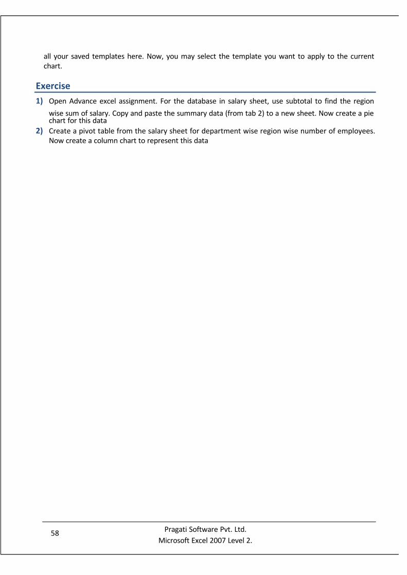
7/14/2019 Excel Level
http://slidepdf.com/reader/full/excel-level 62/76
58Pragati Software Pvt. Ltd.
Microsoft Excel 2007 Level 2.
all your saved templates here. Now, you may select the template you want to apply to the current
chart.
Exercise
1) Open Advance excel assignment. For the database in salary sheet, use subtotal to find the region
wise sum of salary. Copy and paste the summary data (from tab 2) to a new sheet. Now create a piechart for this data
2) Create a pivot table from the salary sheet for department wise region wise number of employees.
Now create a column chart to represent this data
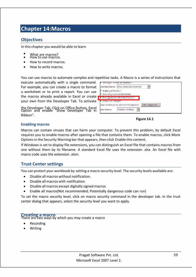
7/14/2019 Excel Level
http://slidepdf.com/reader/full/excel-level 63/76
59Pragati Software Pvt. Ltd.
Microsoft Excel 2007 Level 2.
Chapter 14:Macros
Objectives
In this chapter you would be able to learn
What are macros? How to use macros.
How to record macros.
How to write macros.
You can use macros to automate complex and repetitive tasks. A Macro is a series of instructions that
execute automatically with a single command.
For example, you can create a macro to format
a worksheet or to print a report. You can use
the macros already available in Excel or create
your own from the Developer Tab. To activate
the Developer Tab, Click on Office Button, ExcelOption and enable "Show Developer Tab in
Ribbon".
Enabling macros
Macros can contain viruses that can harm your computer. To prevent this problem, by default Excel
requires you to enable macros after opening a file that contains them. To enable macros, click More
Options in the Security Warning bar that appears, then click Enable this content.
If Windows is set to display file extensions, you can distinguish an Excel file that contains macros from
one without them by its filename. A standard Excel file uses the extension .xlsx. An Excel file with
macro code uses the extension .xlsm.
Trust Center settings
You can protect your workbook by setting a macro security level. The security levels available are:
Disable all macros without notification.
Disable all macros with notification.
Disable all macros except digitally signed macros
Enable all macros(Not recommended; Potentially dangerous code can run)
To set the macro security level, click on macro security command in the developer tab. In the trust
center dialog that appears, select the security level you want to apply.
Creating a macroThere are two ways by which you may create a macro
Recording
Writing
Figure 14.1

7/14/2019 Excel Level
http://slidepdf.com/reader/full/excel-level 64/76
60Pragati Software Pvt. Ltd.
Microsoft Excel 2007 Level 2.
Figure 14.4
Recording a Macro
To record a macro:
1) Click Macro Recording in the status bar to open the Record Macro
dialog box.
2) Specify a name for the macro and a shortcut key. Macronames must begin with a letter and cannot contain spaces.
They can include letters, numbers, and underscores.
3) Click OK to start recording the macro.
4) Perform the actions you want to include in the macro. As you
work, Excel records the sequence of steps.
When you’re finished, click the Stop Recording button on the
status bar.
Store In
This field in the Record macro dialog box, specify where the macro to be recorded will be stored.
There are three options you can select from.Personal Macro Workbook: This workbook, named PERSONAL.XLS, is automatically opened and
hidden, each time you start Excel. This is a good place to store macros that you want available at all
times.
This Workbook: Place the macro in the active workbook. If there is no active workbook, this option is
not available.
New Workbook: A new workbook will be created, and the macro will be recorded in it.
Running a Macro Using Menu Commands
To run a macro, click the Play Macro button in the status bar to
open the Macro dialog box, as shown in diagram. Select the macro
of your choice, and click the Run button
Macros that are contained on all currently open workbooks are
displayed in the list. To run a macro, select macro from the list and
click Run. The Macro dialog box provides several additional
capabilities:
Step
Click this button to run the macro step by step. Stepping through a
macro is useful for debugging purposesEdit The module containing the macro is activated, and the macro is
displayed in the visual basic editor for editing purposes.
DeleteDeletes the selected macro. (You can also delete macros by activating
the module and clearing the macro.)
OptionsLets you assign a shortcut key, add a command to Excel's Tools menu
that runs the macro, and change the description of the macro.
Figure 14.2
Figure 14.3

7/14/2019 Excel Level
http://slidepdf.com/reader/full/excel-level 65/76
61Pragati Software Pvt. Ltd.
Microsoft Excel 2007 Level 2.
Viewing the recorded Macro
As mentioned in the table above, from the macro dialog box, we can edit or step into a macro's code.
Clicking on either of these options opens the visual basic editor. The visual basic editor layout is
shown in figure 14.5.
The above image shows the editor when book1 is open. If you have macros in this workbook, you
would see an additional folder in the project explorer called "Modules". All macros in a file are stored
in Modules. These modules are by default named as Module1, Module2 etc.
Writing a macro
A macro can be written inside a module. To insert a new module into a file right click on the file name
in the project explorer, click on insert and select module. Double clicking on the last module createdwill open it. You may start writing you macro here.
VBA can be used to create
1) A Sub Procedure (Macro)
2) User Defined functions
Figure 14.5
Menu Bar
Project Explorer
Properties Window

7/14/2019 Excel Level
http://slidepdf.com/reader/full/excel-level 66/76
62Pragati Software Pvt. Ltd.
Microsoft Excel 2007 Level 2.
Creating a sub procedure
A recorded macro is a sub procedure. Thus if you wish to have a macro like the one recorded (to be
able to run it from the macro dialog box), you have to write the code in the sub block. The syntax of a
sub block is as follows
Sub procedure_name()
End Sub
Procedure name must begin with a letter and cannot contain spaces. It can include letters, numbers,
and underscores.
For example, given below are two procedures Upcase and lowcase. They convert data in the selected
cells to upper case and lowercase respectively.
Sub ucase()For each cell In Selection
cell.Value = ucase(cell.Value)
Next
End Sub
---------------------------------------------------------------------------------------------------------------------------------------
Sub lowcase()
For each cell In Selection
cell.Value = lcase(cell.Value)
Next
End Sub
Tip: If you write Sub and the procedure name in a module and press enter, end sub comes
automatically.
Display alerts or messages using sub procedures
If you need to display messages or alerts using sub procedures, you may use the msgbox object. The
syntax for a message box is as follows
Msgbox "message"
For example, msgbox "Hello!" will give a message box which says “Hello!”. To concatenate a variableyou may use "&" symbol.

7/14/2019 Excel Level
http://slidepdf.com/reader/full/excel-level 67/76
63Pragati Software Pvt. Ltd.
Microsoft Excel 2007 Level 2.
Example:
Sub message()
Name="Pragati"
Msgbox "Hello!" & name
End sub
Accept inputs using sub procedures
In the above example, if you need to take the name from the user while the sub procedure is run, you
may use inputbox object. The syntax of inputbox is as follows
Inputbox ("message")
Example
Name=Inputbox("Enter the name")
This would accept a name from the user and save it in the variable name. Thus to make the above
example even more dynamic, that is to take the name from the user and display a message box with
the name, you may use the following code
Sub message()
Name=Inputbox("Enter the name")
Msgbox "Hello!" & name
End sub
Creating a function
If use a complex formula frequently and wish to have a function that represents the formula so that itbecomes easier to use it, you may define the function using the visual basic editor.
A function is written in the function block. The syntax of function block is as follows
Functionfunction_name(parameter1,parameter2,……)
End function
Parameters are inputs to a function. If you want that your function take two inputs, you can have two
parameters. These parameters would be variables that would store the values you accept as input.
Note: Variables are memory areas that hold value. Eg: a=2 here a is a variable that holds the value 2
Once defined, you may use a user defined function like you use any worksheet function. In the
functions list dialog box, you can find the new function under user defined functions.
For example, given below is a sample function to calculate profit.

7/14/2019 Excel Level
http://slidepdf.com/reader/full/excel-level 68/76
64Pragati Software Pvt. Ltd.
Microsoft Excel 2007 Level 2.
Using conditions in a function
To use conditions in a function, you may want to do a calculation where, tax is calculated as follows,
Tax is 5% of salary if salary is less than 5000, 7% if salary is between 5000 and 10000 and for all the
others it is 10%. To do this in a function, use the "If---Else--Endif" block. The syntax for the same is as
follows
Syntax
If condition then
Statement
ElseStatement
Endif
Here, else is an optional syntax. There may exist an If-Endif block without an else. If there are multiple
conditions, you may use Elseif instead of else. The syntax of if with Elsif is as follows,
Syntax
If condition then
Statement
Elseif
Statement
Endif
Using the discussed concept, the scenario discussed earlier can be solved as below
Function Profit (sp,cp)
Profit=sp-cpEnd function
Function Usage
Figure 14.6

7/14/2019 Excel Level
http://slidepdf.com/reader/full/excel-level 69/76
65Pragati Software Pvt. Ltd.
Microsoft Excel 2007 Level 2.
Assigning a Macro to a Button
Having created macros using the discussed methods, there are several ways to run a macro. One of
them is to assign a macro to a button in the Quick Access
Toolbar. After assigning the macro to a button, you canrun it by clicking that button.
To assign a macro to a button:
Click the options menu on the Quick Access Toolbar, and
select Customize Quick Access Toolbar. The Application
Settings dialog box opens with the Customization pane
displayed.
From the Available commands list, select Macros.
Select the macro to add to the toolbar and click Add >>.
Click OK to close the Application Settings dialog box
Function Ptax(sal)
If sal< 5000 Then
Ptax = sal * .05
ElseIfsal> 5000 And sal<= 10000 Then
Ptax = sal * .07Else: Ptax = sal * .1
End If
End Function
Figure 14.7

7/14/2019 Excel Level
http://slidepdf.com/reader/full/excel-level 70/76
66Pragati Software Pvt. Ltd.
Microsoft Excel 2007 Level 2.
Final Assignment
Salary statement for the month of April
Open Final Assignment Sheet In the assignments workbook and solve the below questions
1) Calculate DA for Officer 10%, Manager 15%, & Clerk 5% of Basic (using Vlookup).
2) Calculate HRA as following condition (using If condition)
For Officer 1000, Manager 1500, Clerk 500
3) Calculate Conveyance 10 % of Basic using (Range Name)
4) Calculate Gross [ie Basic + DA +HRA+CONV]
5) Calculate ESIC according to Slab-wise on Basic as follows(using Vlookup)
From 0 - 1000 = 50
1001 - 3000 = 100 3001 - 5000 = 250
>5000 = 300
6) Calculate Tax according to Slab-wise on Gross (using if function)
i.e. <10000 = 0
>10000 &<15000 = 750
>15000 = 1500
7) Calculate P.F as 5 % on Basic Salary
8) Calculate Loan 2% of Gross
9) Calculate Net Salary ie [Gross-[ESIC+IT+PF+LOAN]]
Make multiple copies of the Worksheet and solve the following questions in different sheets. Name
the sheets with question number example answer to question number 10 would be solved in the
worksheet name q10.
10) Create a Chart of Name, Basic, Gross & Net [Should be well formatted]
11) Sort your Records Desg wise. [ie Manager then officer and then clerk] [ Custom Sort]
EMPNO NAME DESG Branch BASIC
1 RAJ OFFICER Mumbai 5000
2 RAJESH CLERK Mumbai 3500
3 ANAND MANAGER Delhi 7000
4 RAJU CLERK Delhi 4000
5 HEMANT MANAGER Mumbai 8000
6 SANTOSH CLERK Delhi 3780
7 BHAUMIK OFFICER Delhi 4200
8 MANJIT OFFICER Mumbai 5000
9 KAMAL OFFICER Delhi 3800
10 SONU CLERK Mumbai 2500
7/14/2019 Excel Level
http://slidepdf.com/reader/full/excel-level 71/76
67Pragati Software Pvt. Ltd.
Microsoft Excel 2007 Level 2.
12) Display only the records of Clerk & Manager [Using Auto Filter].
13) Display the Records of those people whose Net Salary is between 1000 –3000 and 6000-9000 and
get the result on a new page [Using Advance Filter].
14) Get the total salary branch wise by subtotal [Using Subtotal Command].
15) Create a Pivot Report Branch wise, Designation wise Net Salary & count the No of Employee.
16) Freeze the Name column & the heading of the data. [Using Freeze Pane].17) Highlight the Entire Row where the Designation = Manager [Using Conditional Formatting].
18) Protect the Whole sheet in such a fashion that you can make changes in Salary column and all the
formula should be lock and hidden.
19) Create a Scenario of Increment for Kamal and Sonu in their basic Salary by 5000 and find out what
will be the Net salary.
20) Give Password to the File as Final.

7/14/2019 Excel Level
http://slidepdf.com/reader/full/excel-level 72/76
68Pragati Software Pvt. Ltd.
Microsoft Excel 2007 Level 2.
Shortcuts In Excel 2007
Shortcut Command
CTRL combination shortcut keys Microsoft Excel 2007
CTRL+SHFT+( Unhide any hidden rows within the selection.
CTRL+SHFT+) Unhide any hidden columns within the selection.
CTRL+SHFT+& Applies the outline border to the selected cells.
CTRL+SHFT_ Removes the outline border from the selected cells.
CTRL SHFT ~ Applies the General number format in Microsoft Excel.
CTRL+SHFT+$Applies the Currency format with two decimal places (negative numbers in
parentheses).
CTRL+SHFT+% Applies the Percentage format with no decimal places.
CTRL+SHFT+^ Applies the Exponential number format with two decimal places.
CTRL+SHFT+# Applies the Date format with the day, month, and year.
CTRL+SHFT+@ Applies the Time format with the hour and minute, and AM or PM.
CTRL+SHFT+!Applies the Number format with two decimal places, thousands separator, and
minus sign (-) for negative values.
CTRL+SHFT+*Selects the current region around the active cell (the data area enclosed by blank
rows and blank columns). In a PivotTable, it selects the entire PivotTable report.
CTRL+SHFT+: Enters the current time.
CTRL+SHFT+Copies the value from the cell above the active cell into the cell or the Formula
Bar.
CTRL SHFT Plus ( ) Displays the Insert dialog box to insert blank cells in Microsoft Excel.
CTRL+Minus (-) Displays the Delete dialog box to delete the selected cells.
CTRL+; Enters the current date.
CTRL+`Alternates between displaying cell values and displaying formulas in the
worksheet.
CTRL+'Copies a formula from the cell above the active cell into the cell or the Formula
Bar.
CTRL+1 Displays the Format Cells dialog box.

7/14/2019 Excel Level
http://slidepdf.com/reader/full/excel-level 73/76
69Pragati Software Pvt. Ltd.
Microsoft Excel 2007 Level 2.
CTRL+2 Applies or removes bold formatting.
CTRL+3 Applies or removes italic formatting.
CTRL 4 Applies or removes underlining in Microsoft Excel.
CTRL+5 Applies or removes strikethrough.
CTRL+6Alternates between hiding objects, displaying objects, and displaying
placeholders for objects.
CTRL+8 Displays or hides the outline symbols.
CTRL+9 Hides the selected rows.
CTRL 0 Hides the selected columns in Microsoft Excel.
CTRL+A
Selects the entire worksheet. If the worksheet contains data, CTRL+A selects the
current region. Pressing CTRL+A, a second time selects the current region and itssummary rows. Pressing CTRL+A a third time selects the entire worksheet. When
the insertion point is to the right of a function name in a formula, displays the
Function Arguments dialog box. CTRL+SHFT+A, inserts the argument names and
parentheses when the insertion point is to the right of a function name in a
formula.
CTRL+B Applies or removes bold formatting.
CTRL+CCopies the selected cells. CTRL+C followed by another CTRL+C, displays the
Clipboard.
CTRL+DUses the Fill Down command to copy the contents and format of the topmost
cell of a selected range into the cells below.
CTRL+FDisplays the Find and Replace dialog box, with the Find tab selected. WhileSHFT+F5 also display this tab, SHFT+F4,repeats the last Find action.
CTRL+SHFT+F, opens the Format Cells dialog box with the Font tab selected.
CTRL+G Displays the Go To dialog box. F5 also displays this dialog box.
CTRL+H Displays the Find and Replace dialog box, with the Replace tab selected.
CTRL I Applies or removes italic formatting in Microsoft Excel.
CTRL+KDisplays the Insert Hyperlink dialog box for new hyperlinks or the Edit Hyperlink
dialog box for selected existing hyperlinks.
CTRL+N Creates a new, blank workbook.
CTRL ODisplays the Open dialog box to open or find a file. CTRL SHFT O selects all cells
that contain comments in Microsoft Excel.
CTRL+P Displays the Print dialog box. CTRL+SHFT+P, opens the Format Cells dialog boxwith the Font tab selected.
CTRL+RUses the Fill Right command to copy the contents and format of the leftmost cell
of a selected range into the cells to the right.
CTRL+S Saves the active file with its current file name, location, and file format.
CTRL T Displays the Create Table dialog box in Microsoft Excel.
CTRL+U Applies or removes underlining. CTRL+SHFT+U switches between expanding and
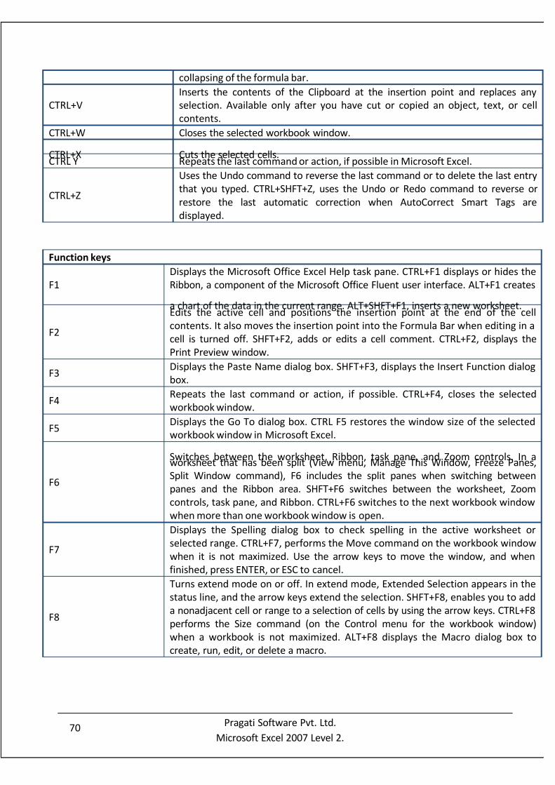
7/14/2019 Excel Level
http://slidepdf.com/reader/full/excel-level 74/76
70Pragati Software Pvt. Ltd.
Microsoft Excel 2007 Level 2.
collapsing of the formula bar.
CTRL+V
Inserts the contents of the Clipboard at the insertion point and replaces any
selection. Available only after you have cut or copied an object, text, or cell
contents.
CTRL+W Closes the selected workbook window.
CTRL+X Cuts the selected cells.CTRL Y Repeats the last command or action, if possible in Microsoft Excel.
CTRL+Z
Uses the Undo command to reverse the last command or to delete the last entry
that you typed. CTRL+SHFT+Z, uses the Undo or Redo command to reverse or
restore the last automatic correction when AutoCorrect Smart Tags are
displayed.
Function keys
F1
Displays the Microsoft Office Excel Help task pane. CTRL+F1 displays or hides the
Ribbon, a component of the Microsoft Office Fluent user interface. ALT+F1 creates
a chart of the data in the current range. ALT+SHFT+F1, inserts a new worksheet.
F2
Edits the active cell and positions the insertion point at the end of the cell
contents. It also moves the insertion point into the Formula Bar when editing in a
cell is turned off. SHFT+F2, adds or edits a cell comment. CTRL+F2, displays the
Print Preview window.
F3Displays the Paste Name dialog box. SHFT+F3, displays the Insert Function dialog
box.
F4Repeats the last command or action, if possible. CTRL+F4, closes the selected
workbook window.
F5Displays the Go To dialog box. CTRL F5 restores the window size of the selected
workbook window in Microsoft Excel.
F6
Switches between the worksheet, Ribbon, task pane, and Zoom controls. In aworksheet that has been split (View menu, Manage This Window, Freeze Panes,
Split Window command), F6 includes the split panes when switching between
panes and the Ribbon area. SHFT+F6 switches between the worksheet, Zoom
controls, task pane, and Ribbon. CTRL+F6 switches to the next workbook window
when more than one workbook window is open.
F7
Displays the Spelling dialog box to check spelling in the active worksheet or
selected range. CTRL+F7, performs the Move command on the workbook window
when it is not maximized. Use the arrow keys to move the window, and when
finished, press ENTER, or ESC to cancel.
F8
Turns extend mode on or off. In extend mode, Extended Selection appears in the
status line, and the arrow keys extend the selection. SHFT+F8, enables you to add
a nonadjacent cell or range to a selection of cells by using the arrow keys. CTRL+F8
performs the Size command (on the Control menu for the workbook window)
when a workbook is not maximized. ALT+F8 displays the Macro dialog box to
create, run, edit, or delete a macro.

7/14/2019 Excel Level
http://slidepdf.com/reader/full/excel-level 75/76
71Pragati Software Pvt. Ltd.
Microsoft Excel 2007 Level 2.
Other useful shortcut keys
ARROW KEYS
Move one cell up, down, left, or right in a worksheet. CTRL+ARROW KEY moves to
the edge of the current data region (data region: A range of cells that contains data
and that is bounded by empty cells or datasheet borders.) in a worksheet.
SHFT+ARROW KEY, extends the selection of cells by one cell. CTRL+SHFT+ARROW
KEY extends the selection of cells to the last nonblank cell in the same column or
row as the active cell, or if the next cell is blank, extends the selection to the next
nonblank cell
BACKSPACE
Deletes one character to the left in the Formula Bar in Microsoft Excel. Also clears
the content of the active cell. In cell editing mode, it deletes the character to the left
of the insertion point.
DELETE Removes the cell contents (data and formulas) from selected cells without affectingcell formats or comments. In cell editing mode, it deletes the character to the right
of the insertion point.
END
Moves to the cell in the lower-right corner of the window when SCROLL LOCK is
turned on. Also selects the last command on the menu when a menu or submenu is
visible. CTRL+END moves to the last cell on a worksheet, in the lowest used row of
the rightmost used column. If the cursor is in the formula bar, CTRL+END, moves the
cursor to the end of the text. CTRL+SHFT+END, extends the selection of cells to the
last used cell on the worksheet (lower-right corner). If the cursor is in the formula
bar, CT
ENTER
Completes a cell entry from the cell or the Formula Bar, and selects the cell below
(by default). In a data form, it moves to the first field in the next record. Opens a
selected menu (press F10 to activate the menu bar) or performs the action for a
selected command. In a dialog box, it performs the action for the default command
button in the dialog box (the button with the bold outline, often the OK button).
ALT+ENTER starts a new line in the same cell. CTRL+ENTER fills the selected cell
range
ESCCancels an entry in the cell or Formula Bar in Microsoft Excel. Closes an open menu
or submenu, dialog box, or message window. It also closes full screen mode when
F9
Calculates all worksheets in all open workbooks. SHFT F9 calculates the active
worksheet in Microsoft Excel. CTRL ALT F9 calculates all worksheets in all open
workbooks, regardless of whether they have changed since the last calculation.
CTRL ALT SHFT F9 rechecks dependent formulas, and then calculates all cells in all
open workbooks, including cells not marked as needing to be calculated. CTRL F9
minimizes a workbook window to an icon.
F10
Turns key tips on or off. SHFT F10 displays the shortcut menu for a selected item in
Microsoft Excel. ALT SHFT F10 displays the menu or message for a smart tag. If
more than one smart tag is present, it switches to the next smart tag and displays
its menu or message. CTRL F10 maximizes or restores the selected workbook
window.
F11
Creates a chart of the data in the current range. SHFT+F11, inserts a new
worksheet. ALT+F11 opens the Microsoft Visual Basic Editor, in which you can
create a macro by using Visual Basic for Applications (VBA).
F12 Displays the Save As dialog box.

7/14/2019 Excel Level
http://slidepdf.com/reader/full/excel-level 76/76
this mode has been applied, and returns to normal screen mode to display the
Ribbon and status bar again.
HOME
Moves to the beginning of a row in a worksheet. Moves to the cell in the upper-left
corner of the window when SCROLL LOCK is turned on. Selects the first command
on the menu when a menu or submenu is visible. CTRL+HOME moves to the
beginning of a worksheet. CTRL+SHFT+HOME, extends the selection of cells to thebeginning of the worksheet.
PAGE DOWN
Moves one screen down in a worksheet. ALT+PAGE DOWN moves one screen to the
right in a worksheet. CTRL+PAGE DOWN, moves to the next sheet in a workbook.
CTRL+SHFT+PAGE DOWN, selects the current and next sheet in a workbook.
PAGE UP
Moves one screen up in a worksheet. ALT+PAGE UP moves one screen to the left in
a worksheet. CTRL+PAGEUP, moves to the previous sheet in a workbook.
CTRL+SHFT+PAGEUP, selects the current and previous sheet in a workbook.
SPACEBAR
In a dialog box, performs the action for the selected button, or selects or clears a
check box. CTRL+SPACEBAR, selects an entire column in a worksheet.
SHFT+SPACEBAR, selects an entire row in a worksheet. CTRL+SHFT+SPACEBAR,
selects the entire worksheet. If the worksheet contains data,
CTRL+SHFT+SPACEBAR, selects the current region. Pressing CTRL+SHFT+SPACEBAR a
second time selects the current region and its summary rows. Pressing
CTRL+SHFT+SPACEBAR a third time selects the entire worksheet.
TAB
Moves one cell to the right in a worksheet. Moves between unlocked cells in a
protected worksheet. Moves to the next option or option group in a dialog box.
SHFT TAB moves to the previous cell in a worksheet or the previous option in a
dialog box in Microsoft Excel. CTRL TAB switches to the next tab in dialog box. CTRL
SHFT TAB switches to the previous tab in a dialog box.