Examples to be solved in exercises · x1=sum(fix(5*rand(1,1,'u'))+1);...
27
Transcript of Examples to be solved in exercises · x1=sum(fix(5*rand(1,1,'u'))+1);...
Examples to be solved in exercises
1 Exercise - probability
1.1 Example
// Two dice
// ------------------------------------------
[u,t,n]=file(); chdir(dirname(n(2)));
clc, clear, close, getd func, mode(0)
//What is the probability that sum of the the dashed dices
//will be greater than 3.
nd=10000; // number of experiments
x2=fix(6*rand(2,nd,'u'))+1; // nd throws with two dice
x=sum(x2,1); // sums on dice
s=0;
for i=1:nd // loop for counting positive res.
if x(i)>3
s=s+1;
end
end
P_stat=s/nd // statistical probability
P_class=1-3/36 // classical probability
1.2 Example
// Balls - realization with a function
// ------------------------------------------
[u,t,n]=file(); chdir(dirname(n(2)));
clc, clear, close, getd func, mode(0)
function k=balls(v) // function definition
// drawing a ball
k=(rand(1,1,'u')>(v(1)/sum(v)))+1;
endfunction
//In a box we have 3w and 5b balls. We draw subsequently 2 balls without
//returning the first one. What is the probability that the second drawn
//ball will be white?
nd=10000; // numb. of experiments
nw=3; nb=5; // numb. of baals
s=0;
1
for i=1:nd // loop for experiments
n=[nw nb];
j=balls(n); // first draw
// j=(rand(1,1,'u')>(n(1)/sum(n)))+1;
n(j)=n(j)-1;
j=balls(n); // second draw
// j=(rand(1,1,'u')>(n(1)/sum(n)))+1;
if j==1 // count of positive res.
s=s+1;
end
end
P_stat=s/nd // statistical probability
P_class=3/8 // classical probability
2 Exercise - characteristics
2.1 Example
// Characteristics of r.v.
// ------------------------------------------
[u,t,n]=file(); chdir(dirname(n(2)));
clc, clear, close, getd func, mode(0)
nd=100;
// continuous data
x1=.16*rand(nd,1,'n')+5; // variance = 0.4
x2=.64*rand(nd,1,'n')-3; // variance = 0.8
m1=mean(x1)
m2=mean(x2)
v1=variance(x1)
v2=variance(x2)
cv=covariance(x1,x2) // covariance
cr=corrcoef(x1,x2) // correlation coefficient
// binomial data
y=(rand(nd,1,'u')<.3)+0;
p=sum(y)/nd // ratio
// discrete data
z=fix(10*rand(nd,1,'u'))+fix(5*rand(nd,1,'u'))+1;
me=median(z)
2
[f,s]=histplot(min(z):max(z),z);
[xxx,j]=max(f);
mo=s(j)
2.2 Example
// One dice - conditional prob.
// ------------------------------------------
[u,t,n]=file(); chdir(dirname(n(2)));
clc, clear, close, getd func, mode(0)
//a) What is the probability, that after a roll of a dice we obtain
// odd number?
//b) What is the above probability if we know, that the number
// is less than 5.
//c) What is the probability according to a) if we know, that the number
// is less than 4.
nd=1000;
// a)
s=0;
for i=1:nd
x=fix(6*rand(1,1,'u'))+1;
if x/2~=fix(x/2)
s=s+1;
end
end
Pa=s/nd
// b)
s=0;
for i=1:nd
x=fix(4*rand(1,1,'u'))+1;
if x/2~=fix(x/2)
s=s+1;
end
end
Pb=s/nd
// c)
s=0;
for i=1:nd
x=fix(3*rand(1,1,'u'))+1;
if x/2~=fix(x/2)
s=s+1;
end
end
Pc=s/nd
3
// True prob.
//Pa=1/2
//Pb=1/2
//Pc=2/3
2.3 Example
// Two dice - conditional prob.
// ------------------------------------------
[u,t,n]=file(); chdir(dirname(n(2)));
clc, clear, close, getd func, mode(0)
//a) What is the probability, that after a roll of two dice the sum
// will be odd number?
//b) What is the above probability if we know, that the number on
// the first dice was not six.
//c) What is the probability according to a) if we know, that neither
// on the first nor on the second dice the result was six.
nd=10000;
// a)
s=0;
for i=1:nd
x1=sum(fix(6*rand(1,1,'u'))+1);
x2=sum(fix(6*rand(1,1,'u'))+1);
x=x1+x2;
if x/2~=fix(x/2)
s=s+1;
end
end
Pa=s/nd
// b)
s=0;
for i=1:nd
x1=sum(fix(5*rand(1,1,'u'))+1);
x2=sum(fix(6*rand(1,1,'u'))+1);
x=x1+x2;
if x/2~=fix(x/2)
s=s+1;
end
end
Pb=s/nd
// c)
s=0;
for i=1:nd
4
x1=sum(fix(5*rand(1,1,'u'))+1);
x2=sum(fix(5*rand(1,1,'u'))+1);
x=x1+x2;
if x/2~=fix(x/2)
s=s+1;
end
end
Pc=s/nd
// True prob.
//Pa=1/2
//Pb=1/2
//Pc=12/25=0.48
3 Exercise - generation
3.1 Example
// Generation
// ------------------------------------------
[u,t,n]=file(); chdir(dirname(n(2)));
clc, clear, close, getd func, mode(0)
m=1;
n=1000;
set(scf(),'position',[600 100 800 600]);
x=grand(m,n,'nor',2,.09);
histplot(20,x);
mx=mean(x)
vx=variance(x)
return
// and try others
x = grand(m, n, "bin", N, p);
x = grand(m, n, "geom", p);
x = grand(m, n, "poi", mu);
x = grand(m, n, "nor", Av, Sd);
x = grand(m, n, "exp", Av);
x = grand(m, n, "unf", Low, High);
x = grand(m, n, "gam", shape, rate);
x = grand(m, n, "bet", A, B);
x = grand(m, n, "chi", Df);
x = grand(m, n, "f", Dfn, Dfd);
5

3.2 Example
// Výb¥r 5ti ze 100, kde jsou 3 vadné
// ------------------------------------------
[u,t,n]=file(); chdir(dirname(n(2)));
clc, clear, close, getd func, mode(0)
//In the store, there are 100 bulbs. Three of them are bad.
//Five bulbs are randomly chosen. What is the probability, that at
//least one of the chosen bulbs will be bad?
nd=10000; // number of experiments
s=0;
for i=1:nd
x=fix(100*rand(1,5,'u'))+1; // 5 chosen bulbs
z=sum(x<4);
if z>0 // count of positive
s=s+1;
end
end
P_stat=1-s/nd
P_class=0.856
// P_class=exp(combLn(95,3)-combLn(100,3))
3.3 Example
// Watch randomly stopped
// ------------------------------------------
[u,t,n]=file(); chdir(dirname(n(2)));
clc, clear, close, getd func, mode(0)
//A watch, whose battery was weak, randomly stopped. What is
//the probability, that the big hand was stopped between
//9 and 12 o'clock? What is the probability for the small hand?
nd=10000; // number of experiments
s=0;
for i=1:nd
x=12*rand(1,1,'u'); // watch stopped
if (x>9) & (x<12) // count of positive
s=s+1;
end
end
P_stat=s/nd
P_class=1/4
6

4 Exercise - sample
4.1 Example
// Limit theorems - central L.T.
// - down: dice
// - right: repeated experiments
// a chooses from {dice, coin}
// ------------------------------------------
[u,t,n]=file(); chdir(dirname(n(2)));
clc, clear, close, getd func, mode(0)
nd=10000;
nc=50;
a=6; // 6 - dice, 2 - coin
x=fix(a*rand(nc,nd,'u')+1);
s=sum(x,1);
histplot(20,s);
4.2 Example
// Limit theorems - law of large numbers
// ------------------------------------------
[u,t,n]=file(); chdir(dirname(n(2)));
clc, clear, close, getd func, mode(0)
nd=1000; // numb. of visible steps
h=10; // number of steps within
nc=5; // number of coins
a=6; // 6 - dice, 2 - coin
x=fix(a*rand(nc,nd*h,'u')+1);
s=sum(x,1);
for i=1:nd
c=s(1:i*h);
mc(i)=mean(c); // estimate of mean
vc(i)=variance(c)/(h*i); // variance of estimate
end
vp=mc+sqrt(vc); // upper border
vm=mc-sqrt(vc); // lower border
plot(1:nd,mc,1:nd,vp,':',1:nd,vm,':')
// variance of estimate is var(x)/n
4.3 Example
// Limit theorems - variance of estimate
7

// ------------------------------------------
[u,t,n]=file(); chdir(dirname(n(2)));
clc, clear, close, getd func, mode(0)
ni=10000; // numb. iterations
nd=10;
nc=5; // number of coins
a=6; // 6 - dice, 2 - coin
for i=1:ni
x=fix(a*rand(nc,nd,'u')+1);
s=sum(x,1);
mc(i)=mean(s); // estimate of mean
vc(i)=variance(s);
end
varEst=variance(mc) // variance from repeated experiments
avVar=mean(vc)/nd // theoretical var. - var(x)/n
4.4 Example
// Population and Sample (repeated sampling from population)
// ------------------------------------------
[u,t,n]=file(); chdir(dirname(n(2)));
clc, clear, close, getd func, mode(0)
P=[27 29 42 35 25 33 56 37 21 44 59 43 38 36 28];
k=length(P);
m=100;
n=5;
X=samwr(n,m,P); // m samples of the length n
mP=mean(P); // population mean
vP=variance(P) // population variance
mX=mean(X,1); // sample means (from all samples)
vX=variance(mX) // variance of sample means
vT=vP/n // theoretical var. of samp.means
set(scf(),'position',[400 100 500 400])
plot(1:length(P),P,'rx')
plot([1 k],[mP mP],'r')
plot((1:m)+20,mX,'.')
plot([1 m]+20,[mP mP],'b--')
legend('population','mean estimates','expectation','expectation');
8
5 Exercise - regression
5.1 Example
// Regression - prediction
// ------------------------------------------
[u,t,n]=file(); chdir(dirname(n(2)));
clc,clear,close,mode(0),getd func
// Example 1
// In a factory, dependence of the overall costs 'n'
//( in thousands of $) on the production 'p' has been
// investigated. The following data have been measured
prod = [532 297 378 121 519 613 592 497]; // x
cost = [48 32 42 27 45 51 53 48]; // y
// a) Using linear regression estimate the costs for
// the production 1000 products
// b) For which produciton the costs would be equal
// to $ 100 000.
// estimation of regression line
param=lin_reg(prod,cost) // par=[b1,b0]
// prediction
prod0=1000;
cost_1000=lin_pred(prod0,param)
// back prediction
costs0=100; // in thousands of $
prod_100=(costs0-param(2))/param(1)
//printf '\nVerification by formulas\n'
//printf ------------------------\n\n
//
//mp=mean(prod);
//mc=mean(cost);
//vp2=var(prod);
//vc2=var(cost);
//vpc=cvar(prod,cost);
//
//b1=vpc/vp2
//b0=mc-b1*mp
//
//ypp=b1*prod0+b0
//xpp=(costs0-b0)/b1
//
9
5.2 Example
// Regression analysis
// ------------------------------------------
[u,t,n]=file(); chdir(dirname(n(2)));
clc, clear, close, getd func, mode(0)
// Example 3
// A harmful substance leaked into the container with water.
// Neutralizing agent has been applied and the concentration of the
// harmful substance has been measured at time instants 'x'. The
// measured concentrations 'y' are
xi = [5 12 20 26 29 38 65 126];
yi = [19 17 18 17 17 15 14 7];
// Compute the correlation coefficient of linear regression
// and conclude about its suitability. If suitable, compute
// the parameters of linear regression and estimate when
// the concentration will be zero.
disp 'Correletion coefficient'
r=covariance(xi,yi)/sqrt(variance(xi)*variance(yi))
p=lin_reg(xi,yi); // p=[b1 b0]
yp=p(1)*xi+p(2);
scf(); plot(xi,yi,'x',xi,yp,':o')
disp 'Parameters'
p
disp 'Zero concentration at x0'
y0=0;
x_zero=(y0-p(2))/p(1)
5.3 Example
// Polynomial and exponential regression
// ------------------------------------------
[u,t,n]=file(); chdir(dirname(n(2)));
clc, clear, close, getd func, mode(0)
// Example 5
// At certain process we have measured the data
xi = [5 12 20 26 29 38 40 45];
yi = [9 7 12 12 27 35 44 76];
// Perform the polynomial regression of the order 'k' and
// the exponential regression. Using prediction errors
// decide which type of regression is better.
k = 3;
xx=[min(xi):.1:max(xi)];
10
pp=pol_reg(xi,yi,k);
ypp=pol_pred(xx,pp);
scf(); plot(xi,yi,'x',xx,ypp,'markersize',4)
title 'polynomial'
pe=exp_reg(xi,yi);
yep=exp_pred(xx,pe);
scf(); plot(xi,yi,'x',xx,yep,'markersize',4)
title 'exponential'
ep=yi-pol_pred(xi,pp);
SEp=variance(ep)/variance(yi)
ee=yi-exp_pred(xi,pe);
SEe=variance(ee)/variance(yi)
scf();plot(xi,ep,':.',xi,ee,':.',[min(xi) max(xi)],[0 0],':')
title 'prediction errors'
legend('polynomial','exponential');
5.4 Example
// Multivariate regression
// ------------------------------------------
[u,t,n]=file(); chdir(dirname(n(2)));
clc, clear, close, getd func, mode(0)
// Example 6
// At certain process we have measured the data
x1i = [15 12 11 9 9 8 5 3];
x2i = [3 9 5 11 28 14 32 58];
yi = [9 7 22 12 27 31 44 36];
// Perform multivariate linear regression and test its
// suitability. Use standard error SE.
xi=[x1i' x2i']; // all independent variables
p=lin_reg_n(xi,yi);
yp=lin_pred_n(xi,p);
SE=variance(yi-yp)/variance(yi)
scf();plot(1:length(yi),yi,'.',1:length(yi),yp,'x')
legend('output','prediction');
11
6 Exercise - con�dence intervals
6.1 Example
// Conf. interval for expectation (known variance)
// ------------------------------------------
[u,t,n]=file(); chdir(dirname(n(2)));
clc, clear, close, getd func, mode(0)
// Example 7
// Assume, that the height of children in the age 10 has normal distribution
// with the variance "sig2". Determine the interval al-I, in which the true
// height will be if we have measured the data sample of the length "n" with
// the average "mx".
// The interval determine as a) both-sided, b) left and c) rihgt-sided.
sig2 = 38;
n = 12;
mx = 127.3;
al = .01;
// a) both sided
[lb, ub]=z_int(mx,sig2,n,'b',al);
CI_B=[lb ub]
// b) left sided
[lb, ub]=z_int(mx,sig2,n,'l',al);
CI_L=[lb ub]
// c) right sided
[lb, ub]=z_int(mx,sig2,n,'r',al);
CI_R=[lb ub]
6.2 Example
// Conf. interval for expectation (unknown variance)
// ------------------------------------------
[u,t,n]=file(); chdir(dirname(n(2)));
clc, clear, close, getd func, mode(0)
// Example 8
// Assume, that the height of children in the age 10 has normal distribution.
// Determine the interval al-I, in which the true height will be it we have
// measured the data sample of the length "n" with the average "mx".
// The interval determine as a) both-sided, b) rihgt-sided.
n = 12;
mx = 127.3;
s2x = 38;
al = .01;
12
// both sided
[lb, ub]=t_int(mx,s2x,n,'b',al);
CI_B=[lb ub]
// left sided
[lb, ub]=t_int(mx,s2x,n,'l',al);
CI_L=[lb ub]
// right sided
[lb, ub]=t_int(mx,s2x,n,'r',al);
CI_R=[lb ub]
6.3 Example
// Conf. interval for variance
// ------------------------------------------
[u,t,n]=file(); chdir(dirname(n(2)));
clc, clear, close, getd func, mode(0)
// Example 9
// To learn the accuracy of a method for measuring the volume
// of manganese in the steel we performed independent measurements
// of several samples. We would like to know the border for which it holds
// that only 5% of possibly measured variances will be greater than
// the value of the true variance of the method.
// The measured values are
x = [4.3 2.9 5.1 3.3 2.7 4.8 3.6];
vr=variance(x);
n=length(x);
side='r'; // it is (-inf, ub) - ub is the
al=.05;
[lb, ub]=var_int(vr,n,side,al);
printf('\nThe border is %g\n',ub)
6.4 Example
// CI for variance
// ------------------------------------------
[u,t,n]=file(); chdir(dirname(n(2)));
clc, clear, close, getd func, mode(0)
// Example 10
// At the motorway with recommended speed 80 km/h we monitored
// the speeds of passing cars and obtained data 'xi' and 'ni'
// (values and frequencies). Determine both-sided 'al'-interval
13

// for variance of the speeds.
xi = [60 70 75 80 85 90 110]; // values
ni = [ 3 27 36 29 25 31 8]; // frequencies
al = .05;
pi=ni/sum(ni);
mx=sum(xi.*pi);
vr=sum((xi-mx)^2.*pi);
vr=variancef(xi,ni);
n=sum(ni);
[lb, ub]=var_int(vr,n,'b',al);
CI=[lb ub]
6.5 Example
// Confidence interval for proportion
// ------------------------------------------
[u,t,n]=file(); chdir(dirname(n(2)));
clc, clear, close, getd func, mode(0)
// Example 11
// At the motorway with recommended speed 80 km/h we monitored
// the speeds of passing cars and obtained data 'x'
// Determine both-sided 'al'-interval for the ratio of drivers
// that exceed the recommended speed by more than 'r' km/h.
x = [78 86 65 92 83 92 85 66 42 82 ...
99 92 75 81 66 76 89 76 97 76 ...
75 56 76 78 96 77 86 79 86 93];
al= .05;
r = 3;
n=length(x);
n1=sum(x>(80+r));
p=n1/n;
[lb ub]=prop_int(p,n,'b',al);
CI_B=[lb ub]
[lb ub]=prop_int(p,n,'r',al);
CI_R=[lb ub]
7 Exercise - tests with one variable
7.1 Example
// Test of expectation (known variance)
14
// ------------------------------------------
[u,t,n]=file(); chdir(dirname(n(2)));
clc, clear, close, getd func, mode(0)
// Example 12
// From a set of steel rods with equal nominal length we have chosen
// random choice with the lengths 'x'. The producer guarantees that
// the variance of the lengths is 'sig2'. At the
// significance level 'al' test the assertion of the producer
// that the nominal length of the rods id 'd'.
x = [6.2 7.5 6.9 8.9 6.4 7.1];
d = 6.5;
sig2 = .8;
al = .05;
mu0=d;
av=mean(x);
vr=sig2;
n=length(x);
side='b';
pv=z_test(mu0,av,vr,n,side)
7.2 Example
// Test of expectation (unknown variance)
// ------------------------------------------
[u,t,n]=file(); chdir(dirname(n(2)));
clc, clear, close, getd func, mode(0)
// Example 13
// From a set of steel rods with equal nominal length we have chosen
// random choice with the lengths 'x'. At the
// significance level 'al' test the assertion of the producer
// that the nominal length of the rods id 'd'.
x = [6.2 7.5 6.9 8.9 6.4 7.1];
d = 6.5;
al = .05;
mu0=d;
av=mean(x);
vr=variance(x);
n=length(x);
side='b';
pv=t_test(mu0,av,vr,n,side)
7.3 Example
// Test of variance
15
// ------------------------------------------
[u,t,n]=file(); chdir(dirname(n(2)));
clc, clear, close, getd func, mode(0)
// Example 15
// The accuracy of setting of certain machine can be verified
// according to the variance of the products. If the variance is
// greater then the level 'sig2', it is necessary to perform new setting.
// A data sample has been meaasured with values 'mx' and
// frequencies of values 'nx'. On the level 'al' test if it is necessary
// to set the machine.
nx = [ 5 12 32 11 8 3];
mx = [95 100 105 110 115 120];
sig2 = 28;
al = .05;
vr0=sig2;
vr=variancef(mx,nx);
n=sum(nx);
side='r';
pv=var_test(vr0,vr,n,side)
// Note
// H0: var<var0; HA: var>var0
7.4 Example
// Test of proportion
// ------------------------------------------
[u,t,n]=file(); chdir(dirname(n(2)));
clc, clear, close, getd func, mode(0)
// Example 18
// At the motorway with recommended speed 80 km/h we monitored
// the speeds of passing cars and obtained data 'x'.
// At the level 'al' test the hypothesis: The ratio of drivers
// that exceed the recommended speed by more than 'r' km/h is not
// greater than 'P'%
x = [78 86 65 92 83 92 85 66 42 82 ...
99 92 75 81 66 76 89 76 97 76 ...
75 56 76 78 96 77 86 79 86 93];
al= .05;
r = 3;
P = 20;
n=length(x);
m=sum(x>80+r);
p=m/n;
p0=P/100;
16

side='r';
pv=prop_test(p0,p,n,side)
8 Exercise - tests with two variables
8.1 Example
// Test of two expectations (equal variances)
// ------------------------------------------
[u,t,n]=file(); chdir(dirname(n(2)));
clc, clear, close, getd func, mode(0)
// Example 16
// Solidity of materials is verified by two methods A and B.
// The same material has been subdued testing by both methods.
// The results are 'xA' a 'xB'. On the level 'al' test equality of
// both methods. The variability of methods is assumed to be equal.
xA = [20.1 19.6 20.0 19.9 20.1];
xB = [20.9 20.1 20.6 20.5 20.7 20.5];
al = .05;
av1=mean(xA);
vr1=variance(xA);
n1=length(xA);
av2=mean(xB);
vr2=variance(xB);
n2=length(xB);
side='b';
pv=t_test_2s(av1,vr1,n1,av2,vr2, n2,side)
8.2 Example
// Test of two expectations (paired)
// ------------------------------------------
[u,t,n]=file(); chdir(dirname(n(2)));
clc, clear, close, getd func, mode(0)
// Example 17
// We are going to test if the tire removal on left and right sides
// of the front wheels of cars is equal. The measured values are 'xL' a 'xP'.
// Test at the level 'al'.
xL = [1.8 1.0 2.2 0.9 1.5];
xP = [1.5 1.1 2.0 1.1 1.4];
al = .05;
sample1=xL;
sample2=xP;
17
side='b';
pv=t_test_2p(sample1,sample2,side)
8.3 Example
// Test of two expectations (independent)
// ------------------------------------------
[u,t,n]=file(); chdir(dirname(n(2)));
clc, clear, close, getd func, mode(0)
// Example 19
// At the motorway with recommended speed 80 km/h we monitored
// the speeds of cars going into the town and from the town. We
// obtained data 'rD' (speeds into), 'nD' (frequencies into) and
// 'rZ' (speeds from) 'nZ' (frequencies from). At the level 'al'
// test the hypothesis: From the town the cars go more quickly.
nD = [ 5 11 17 65 98 73 79 63 3];
rD = [65 70 75 80 85 90 95 100 110];
nZ = [ 8 22 13 71 48 64 89 24 5];
rZ = [65 70 75 80 85 90 95 100 110];
al = .01;
av1=meanf(rD,nD);
av2=meanf(rZ,nZ);
vr1=variancef(rD,nD);
vr2=variancef(rZ,nZ);
n1=sum(nD);
n2=sum(nZ);
side='r';
pv=t_test_2n(av1,vr1,n1,av2,vr2, n2,side)
// H0: from > into
// HA: from < into --> into - from > 0 -- 'r'
8.4 Example
// Test of two expectations (paired)
// ------------------------------------------
[u,t,n]=file(); chdir(dirname(n(2)));
clc, clear, close, getd func, mode(0)
// Example 20
// During a check of the front lights of cars we have measured
// the data 'xL' (left light) and 'xP' (right light). The values
// are distances (in cm) above (positive) and below (negative) of the
// real level with respect to the optimal level. At the level 'al'
// test if the light levels at each car are the same.
xP = [-3 5 16 9 -8 -2 23 5 -6 -3];
18
xL = [-5 -12 22 -3 -9 1 -1 2 -13 -5];
al = .1;
sample1=xP;
sample2=xL;
side='b';
pv=t_test_2p(sample1,sample2,side)
8.5 Example
// Test of two expectations (paired)
// ------------------------------------------
[u,t,n]=file(); chdir(dirname(n(2)));
clc, clear, close, getd func, mode(0)
// Example 21
// During a check of the front lights of cars we have measured
// the data 'xL' (left light) and 'xR' (right light). The values
// are distances (in cm) above (positive) and below (negative) of the
// real level with respect to the optimal level. At the level 'al'
// test the hypothesis: Left lights are higher than right.
xR = [-3 5 16 9 -8 -2 23 5 -6 -3];
xL = [-5 -12 22 -3 -9 1 -1 2 -13 -5];
al = .1;
sample1=xR;
sample2=xL;
side='r';
pv=t_test_2p(sample1,sample2,side)
8.6 Example
// Test of two proportions
// ------------------------------------------
[u,t,n]=file(); chdir(dirname(n(2)));
clc, clear, close, getd func, mode(0)
// Example 22
// At a crossroads we have written down numbers of cars going
// stright (S) turning to left (L) and right (R). The measured
// data are 'xS', 'xL' a 'xR'.
// On the level 'al' test assertion that the ratio of cars
// going straight is equal to those that are turning .
xS = 62;
xL = 39;
xR = 46;
al = .1;
19
n=xS+xL+xR;
p1=xS/n; // ratio of going stright
n1=xS;
p2=(xL+xR)/n; // ratio of turning
n2=xL+xR;
side='b';
pv=prop_test_2(p1,n1,p2,n2,side)
8.7 Example
// Test of two expectations
// ------------------------------------------
[u,t,n]=file(); chdir(dirname(n(2)));
clc, clear, close, getd func, mode(0)
// Example 23
// At a crossroads during 6 days we have written down numbers
// of cars going stright (R) turning to left (L) anf right (P).
// The measured data are 'xR', 'xL' a 'xP'.
// On the level 'al' test assertion that the number of cars
// going straight is smaller than that of cars turning .
xS = [82 78 92 83 99 97];
xL = [29 42 34 38 45 34];
xR = [31 44 36 54 31 24];
al = .05;
av1=mean(xS);
av2=mean(xL+xR);
vr1=variance(xS);
vr2=variance(xL+xR);
n1=sum(xS);
n2=sum(xL+xR);
side='r';
pv=t_test_2n(av1,vr1,n1,av2,vr2, n2,side)
9 Exercise - testes with many variables
9.1 Example
// Anova 1
// ------------------------------------------
[u,t,n]=file(); chdir(dirname(n(2)));
clc, clear, close, getd func, mode(0)
// Example 24
// We monitor three machines. Randomly, we measure their productions
// per hour 'x1', 'x2' and 'x3. At the level 'al', test the equality
20
// of their production.
al = 0.05;
x1 = [53 55 49 58 52 61 56 55];
x2 = [49 56 52 45 51 56 44 51];
x3 = [52 53 52 54 55 53 53 52];
x=[x1' x2' x3'];
pv=anova_1(x)
9.2 Example
// Anova 1
// ------------------------------------------
[u,t,n]=file(); chdir(dirname(n(2)));
clc, clear, close, getd func, mode(0)
// Example 25
// For one month, we monitor number of accidents at five crossroads.
// The results are in the following table.
// ---------------------------------
// year: 1999 2000 2001 2002 2003
num_1 =[3 5 2 1 3];
num_2 =[6 2 5 3 4];
num_3 =[3 2 1 1 2];
num_4 =[4 1 1 2 2];
num_5 =[4 2 5 5 6];
// --------------------------------
// At the level 'al' test hypothesis: The average number of accidents
// is equal at all monitored crossroads.
al = 0.01;
x=[num_1' num_2' num_3' num_4' num_5'];
disp 'One-way anova'
pv=anova_1(x)
disp 'Two-ways anova'
[pv_col, pv_row]=anova_2(x);
disp(pv_col,'Equality in crossoads')
disp(pv_row,'Equality in time')
9.3 Example
// Chi-square test of uniformity
// ------------------------------------------
[u,t,n]=file(); chdir(dirname(n(2)));
clc, clear, close, getd func, mode(0)
// Example 26
21
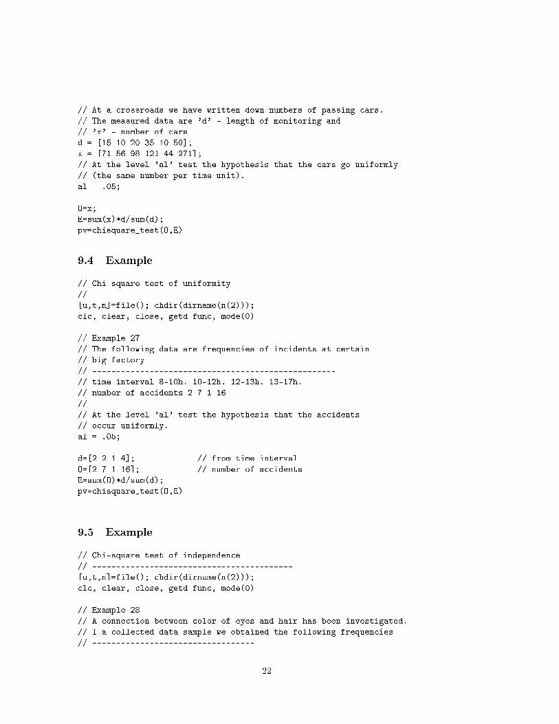
// At a crossroads we have written down numbers of passing cars.
// The measured data are 'd' - length of monitoring and
// 'x' - number of cars
d = [15 10 20 35 10 50];
x = [71 56 98 121 44 271];
// At the level 'al' test the hypothesis that the cars go uniformly
// (the same number per time unit).
al = .05;
O=x;
E=sum(x)*d/sum(d);
pv=chisquare_test(O,E)
9.4 Example
// Chi-square test of uniformity
// ------------------------------------------
[u,t,n]=file(); chdir(dirname(n(2)));
clc, clear, close, getd func, mode(0)
// Example 27
// The following data are frequencies of incidents at certain
// big factory
// ---------------------------------------------------
// time interval 8-10h. 10-12h. 12-13h. 13-17h.
// number of accidents 2 7 1 16
// ---------------------------------------------------
// At the level 'al' test the hypothesis that the accidents
// occur uniformly.
al = .05;
d=[2 2 1 4]; // from time interval
O=[2 7 1 16]; // number of accidents
E=sum(O)*d/sum(d);
pv=chisquare_test(O,E)
9.5 Example
// Chi-square test of independence
// ------------------------------------------
[u,t,n]=file(); chdir(dirname(n(2)));
clc, clear, close, getd func, mode(0)
// Example 28
// A connection between color of eyes and hair has been investigated.
// I a collected data sample we obtained the following frequencies
// ----------------------------------
22

// eyes \ hair light brown dark
// blue 90 75 55
// gray 96 136 88
// brown 108 135 119
// ---------------------------------
// At the level 'al' test the hypothesis that the color of eyes
// and hair are independent.
al = .05;
T=[90 75 55
96 136 88
108 135 119];
pv=chisquare_test_i(T)
10 Exercise - nonparametric tests
10.1 Example
// Mann Whitney test
// ------------------------------------------
[u,t,n]=file(); chdir(dirname(n(2)));
clc, clear, close, getd func, mode(0)
// Example 30
// Two doctors recommend curing the cold with two different
// methods. The results (number of days of the treatment) are
// 'x1' and 'x2'. Test equality of the methods.
x1=[5 8 7 8 4 5 5 6 9 3 5 8 6];
x2=[3 4 9 5 4 9 9 8];
// If needed, add the additionally measured data:
//x1_add=[8 7 5 8 5 7 5 6 8 4 7 7 5 6];
//v2_add=[3 3 5 3 6 4 5 6 2 2 3 4 2 3];
pv=mannwhit_test(x1,x2)
10.2 Example
// Willcoxon test
// ------------------------------------------
[u,t,n]=file(); chdir(dirname(n(2)));
clc, clear, close, getd func, mode(0)
// Example 31
// Eight sportsmen in certain sport club were tested with respect
// to their performance. All of them threw a javelin once and then
// they were subdued to intensive training. Then they threw once more.
// The measured lengths were x1 and x2.
23

// The hypothesis is that one day of training is not enough to
// improve their performance. Test on the level 'al'.
x1=[68 81 69 72 66 91 98 89 75 68 69 75 72 83 88 79 88 76 81 85];
x2=[79 62 70 75 68 81 85 94 71 62 81 70 74 85 82 91 85 82 83 73];
sm='l';
pv=wilcoxon_test(x1,x2,sm)
// Note
// H0: x2 is not greater than x1 ... x2 <= x1
// HA: x1 < x2 left
10.3 Example
// Willcoxon test
// ------------------------------------------
[u,t,n]=file(); chdir(dirname(n(2)));
clc, clear, close, getd func, mode(0)
// Example 32
// Test if mice and stags have equally long front legs. The measured
// values are
x1=[135 123 3.1 2.5 98 124 131 3.4 2.8 128];
x2=[136 121 2.9 2.6 101 121 130 3.5 2.9 126];
// Additionaly measured data
//x1_add=[154 135 2.9 137 2.7 3.0 3.2 131 2.8 148];
//x2_add=[162 141 2.8 142 2.9 2.8 3.0 132 3.1 151];
sm='b';
pv=wilcoxon_test(x1,x2,sm)
10.4 Example
// Friedman test
// ------------------------------------------
[u,t,n]=file(); chdir(dirname(n(2)));
clc, clear, close, getd func, mode(0)
// Example 33
// Tree inspectors are to evaluate functionality of five fast
// food stands. Each inspector evaluates each stand. The result
// is the table Tab: rows correspond to inspectors, columns columns
// to stands. Evaluation is 1,2,..,10. 10 is the best.
// Test if the quality of the stans is equal.
Tab=[10 8 3 9 7
8 7 5 9 10
8 9 5 7 6];
24
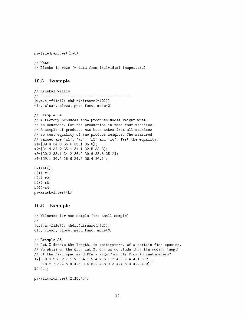
pv=friedman_test(Tab)
// Note
// Blocks in rows (= data from individual inspectors)
10.5 Example
// Kruskal Wallis
// ------------------------------------------
[u,t,n]=file(); chdir(dirname(n(2)));
clc, clear, close, getd func, mode(0)
// Example 34
// A factory produces some products whose weight must
// be constant. For the production it uses four machines.
// A sample of products has been taken from all machines
// to test equality of the product weights. The measured
// values are 'x1', 'x2', 'x3' and 'x4'. Test the equality.
x1=[39.4 34.8 35.6 35.1 35.8];
x2=[34.4 34.2 35.1 31.1 32.5 33.8];
x3=[30.2 35.1 34.2 36.3 30.8 35.6 35.2];
x4=[39.1 34.3 38.6 34.5 36.4 36.1];
L=list();
L(1)=x1;
L(2)=x2;
L(3)=x3;
L(4)=x4;
pv=kruskal_test(L)
10.6 Example
// Wilcoxon for one sample (too small sample)
// ------------------------------------------
[u,t,n]=file(); chdir(dirname(n(2)));
clc, clear, close, getd func, mode(0)
// Example 35
// Let X denote the length, in centimeters, of a certain fish species.
// We obtained the data set X. Can we conclude that the median length
// of the fish species differs significantly from X0 centimeters?
X=[5.0 3.9 8.2 7.5 2.8 4.1 5.4 2.6 1.7 4.3 7.4 4.1 5.2 ..
9.3 2.7 3.4 5.9 4.3 9.4 8.2 4.8 3.3 4.7 5.3 4.2 4.0];
X0=4.1;
pv=wilcoxon_test(X,X0,'b')
25
10.7 Example
// Wilcoxon for one sample (with more data)
// ------------------------------------------
[u,t,n]=file(); chdir(dirname(n(2)));
clc, clear, close, getd func, mode(0)
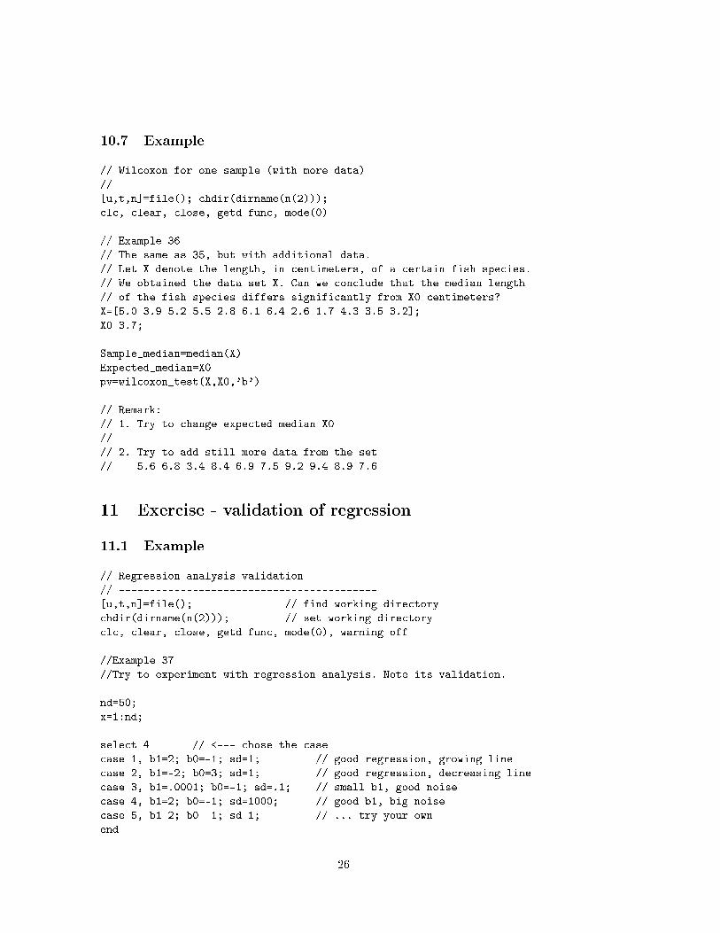
// Example 36
// The same as 35, but with additional data.
// Let X denote the length, in centimeters, of a certain fish species.
// We obtained the data set X. Can we conclude that the median length
// of the fish species differs significantly from X0 centimeters?
X=[5.0 3.9 5.2 5.5 2.8 6.1 6.4 2.6 1.7 4.3 3.5 3.2];
X0=3.7;
Sample_median=median(X)
Expected_median=X0
pv=wilcoxon_test(X,X0,'b')
// Remark:
// 1. Try to change expected median X0
//
// 2. Try to add still more data from the set
// 5.6 6.8 3.4 8.4 6.9 7.5 9.2 9.4 8.9 7.6
11 Exercise - validation of regression
11.1 Example
// Regression analysis validation
// ------------------------------------------
[u,t,n]=file(); // find working directory
chdir(dirname(n(2))); // set working directory
clc, clear, close, getd func, mode(0), warning off
//Example 37
//Try to experiment with regression analysis. Note its validation.
nd=50;
x=1:nd;
select 4 // <--- chose the case
case 1, b1=2; b0=-1; sd=1; // good regression, growing line
case 2, b1=-2; b0=3; sd=1; // good regression, decreasing line
case 3, b1=.0001; b0=-1; sd=.1; // small b1, good noise
case 4, b1=2; b0=-1; sd=1000; // good b1, big noise
case 5, b1=2; b0=-1; sd=1; // ... try your own
end
26
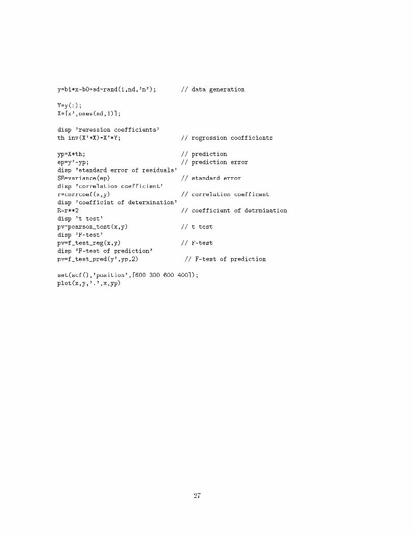
y=b1*x-b0+sd*rand(1,nd,'n'); // data generation
Y=y(:);
X=[x',ones(nd,1)];
disp 'reression coefficients'
th=inv(X'*X)*X'*Y; // regression coefficients
yp=X*th; // prediction
ep=y'-yp; // prediction error
disp 'standard error of residuals'
SE=variance(ep) // standard error
disp 'correlation coefficient'
r=corrcoef(x,y) // correlation coefficent
disp 'coefficint of determination'
R=r**2 // coefficient of detrmination
disp 't-test'
pv=pearson_test(x,y) // t-test
disp 'F-test'
pv=f_test_reg(x,y) // F-test
disp 'F-test of prediction'
pv=f_test_pred(y',yp,2) // F-test of prediction
set(scf(),'position',[600 300 600 400]);
plot(x,y,'.',x,yp)
27


![684.8 [1,1]](https://static.fdocuments.in/doc/165x107/5681611b550346895dd07429/6848-11.jpg)