SEM and AFM Analysis of MWCNTs

Jacob FesteUniversity of Arkansas, Biomedical Engineering, jtfeste@email.uark.edu

1

9/14/2015

2 | P a g e

ABSTRACT

This experiment utilizes the SEM and AFM microscopy techniques to image and characterize Multi-Walled Carbon Nanotubes (MWCNTs). This experiment also provided experience and understanding of the two microscopy techniques, as well as a deeper understanding of nanostructures and the properties correlating to their size at the nanometer scale. The results of this experiment included slight error in SEM imaging at the nanometer scale, likely due to the MWCNTs properties. However, the images were clear enough to determine an estimated outer diameter of 60.9nm and estimated length around 3.21nm. The results from the AFM images were inconclusive, as imaging was made impossible likely due to the preparation of the MWCNTs.

NOMENCLATURE

λ Wavelength (nm)p Electron Momentum (eV)h Plank’s Constant (6.62607004 × 10-34 m2 kg / s)F⃗ Electron Force in Magnetic Field (N)v⃗ Electron Velocity (m/s)B⃗ Magnetic Field Strength (N*s / coulomb*m)e Electron Charge (1.60217662 × 10-19 coulombs)

INTRODUCTION

The primary motivation behind this imaging experiment was to generate a larger understanding of nanostructures, specifically MWCNTs, via various imaging techniques. The imaging techniques performed in this experiment include Scanning Electron Microscopy (SEM) and Atomic Force Microscopy (AFM). While the numerical results of this experiment are centered on the nanostructures themselves, another primary goal of this experiment was to gradually learn and understand these complicated techniques throughout their respective imaging processes.

Even the best optical microscopes are limited to the micrometer scale. This limit is due to the large wavelength of light, even in its smallest form. In microscopy imaging, smaller wavelengths in the particles used to visualize the image generate higher resolution images. This property also relates to the degree of magnification of which microscopy technique can operate, with higher resolutions able to generate images under increased magnification until the quality of the image is diminished [4]. Therefore, microscopy techniques such as the SEM and AFM techniques were uniquely developed to avoid this border in order to reach the nanometer size of a material. Besides their ability to operate at the nanometer scale, the mechanisms behind the SEM and AFM imaging techniques vary significantly. Unlike the AFM technique, the SEM technique generates images by utilizing the chemical properties of a material. The SEM technique, more specifically, takes advantage of the small wavelengths of electrons. The wavelengths of electrons are smaller than those of photons (light) and are given by the following de Broglie relationship:

λ= hp (1)

2

3 | P a g e

Since p represents electron momentum, the relationship indicates that electrons at higher speeds will generate smaller wavelengths and higher resolution images. In addition to smaller electron wavelengths, the SEM technique also takes advantage of the use of electromagnetic lenses [4]. Electrons are inherently non-directional and will randomly occupy the region of space they’re permitted to operate in. The use of electromagnetic lenses allows the SEM technique to “guide” or “focus” electrons down to a small area. This phenomenon is illustrated by the following Lorentz equation [4]:

F⃗=−e (v⃗ × B⃗ ) (2)

Therefore, the inherent directionality generated by magnetic fields allow the SEM focusing process. The final two primary components of the SEM include a vacuum chamber and an electron detector. The principle behind the SEM requires that the measured electrons are able to move larger distances than they normally are able to in air due to their deflection from oxygen and nitrogen atoms. The vacuum chamber is required to eliminate this interaction. The final component, the electron detector, is necessary in order to detect the scattered electrons and generate an image [4]. Each of these components is required for the mechanism of the SEM to succeed. The mechanism of the SEM begins by removing electrons from a source via heat, etc. followed by the focusing of those electrons onto the sample. The electromagnetic lenses focus the high energy electrons through small apertures until the sample is reached. The high energy electron beam results in low energy secondary electrons emitted by the sample due to ionization products. These secondary electrons are then guided to the electron detector and converted into a specific number of flashes of light when reaching the phosphorous light guide on the detector, with increasing electrons giving more flashes. Finally, these flashes of light are converted into an electrical signal that is dependent on the number of flashes detected, producing an image for that small region. This process is repeated as the SEM scans the sample with the electron beam until each region is brought together in a final image shown on the monitor, with slower scans giving higher resolution images. Altogether, SEM microscopy can focus as small as 1-10nm to generate high quality images at the nanometer scale [4]. SEM microscopy operates most efficiently with conductive material, as insulating material acts to resist the release of secondary electrons to give lower resolution images. MWCNTs are composed of carbon, a quite insulated material [5]. It can therefore by hypothesized that SEM imaging will give low resolution images at the nanoscale. The other imaging technique performed in this experiment includes Atomic Force Microscopy (AFM). This technique is much different than the SEM technique in that its ability to operate at the nanoscale level is largely due to the physical properties of a material. It is also able to generate 3D topography maps in addition to 2D images. Fundamentally, the mechanics of the AFM can be explained by Newton’s third law: for every action there is an equal and opposite reaction. This principle hold true at the atomic level. By scanning a sample with a small probe, this technique is able to register the atomic force each region of the sample generates on the probe to form an overall image [4]. The AFM technique contains four key components in order to accomplish this. The “probe” of the AFM is composed of a nano-sized tip attached to a cantilever arm with a piezo scanner at the end of the arm [4]. For this experiment, the “tapping mode” form of AFM was performed. In this mode, the cantilever arm is held near its resonant frequency, oscillating the small tip over the sample as it scans. As the arm approaches the sample, atomic forces on the small tip cause the amplitude of the oscillating arm to decrease.

3

4 | P a g e

Immediately following, the piezo scanner alters the height of the cantilever to maintain its original amplitude. At that moment the final major component, a laser that is constantly reflecting off the top of the cantilever and into photodiodes, registers this displacement in laser position for that region due to the sudden change in cantilever height. Finally, these displacements are converted into electrical signals as the scanning ensues to generate an image on the monitor. This technique is excellent for 3D topography mapping as it gives very high vertical resolutions up to 0.01nm. The horizontal resolution of an AFM image is much less and is dependent on the size of the tip, with smaller tips giving a better resolution [4]. Due to this property, SEM 2D images will likely give better resolution unless the sample is highly insulated. It can therefore be hypothesized that the AFM images (3D and 2D) of MWCNTs will be of higher resolution than the SEM images due to the MWCNTs insulated properties. The shape of MWCNTs includes aromatic rings of carbon in a cylindrical shape [5]. This property also suggests higher quality AFM images, as the vertical aspects of the structure that will be measured in very high resolution will be very similar to the horizontal aspects due to the circular surface. It is also important to note that while the AFM may seem more effective at measuring the specific sample; it is much more difficult and time consuming to operate this technique as locating the sample to place the probe can be tedious. MWCNTs tend to bundle together so this sample may minimize this concern [5]. Nanostructures are very unique in their properties due to their small size, with the smallest changes in size affecting areas such as optical and electrical properties. This aspect gives rise to various imaging techniques being better suited for various nanostructures, even in such a small and seemingly insignificant region of space.

EXPERIMENTAL SETUP

SEM

1. Due to the complex nature of the machine, sample loading and major adjustments were completed by the TA prior to use. Loading was practiced using a Phenom machine.

2. After navigation with the mouse, the magnification and focus knobs (fine and coarse) were adjusted until suitable SEM images were obtained. Maximum resolution is obtained at high magnification when the radius of aperture is minimized and the fine focus knob correlating with the coarse knob generate a minimal beam radius touching the sample.

3. These images were saved and evaluated using the SEM software to determine the estimated diameter and length of the sample.

AFM

1. Due to the complex nature of the machine, sample loading and major adjustments were completed by the TA prior to use.

2. Following the first step, the following parameters independent of the sample structure were adjusted:

Scan Size- Increasing scan size increases the overall size of the image. Scan Rate- Decreasing scan rate increases image resolution.

4

5 | P a g e

Samples/Line- Increased samples/line increase image resolution.

3. The following parameters dependent on the sample structure were also adjusted:

Integral Gain- Determines the degree at which the area under the scanning curve is adjusted by the AFM. This correlates with the proportional gain and is typically a fraction of the proportional gain.

Proportional Gain- Determines the degree at which the AFM adjusts the frequency of the trace and retrace scanning curves, with similar frequencies giving higher resolutions. This gain is typically correlated and much larger than the integral gain due to the integral gain generating larger numbers at smaller gains.

Amplitude Setpoint- Sets the default amplitude of the oscillating cantilever. Samples with more overall height may require a higher amplitude to avoid contact while smaller heights may require smaller amplitudes to generate accurate results.

4. The following parameters were also adjusted relating to the viewing of the image:

Data Scale Data Center Realtime Plane Fit

5. Finally, an image was captured when a suitable scan at a high resolution was obtained. These images were also analyzed for size.

Diagrams

Figure 1: General diagram of AFM and its mechanisms.

5

6 | P a g e

Figure 2: General diagram of SEM and its mechanisms.

DATA AND RESULTS

Figure 3: Image of inside the SEM.

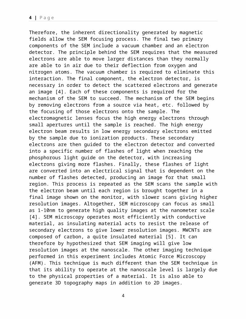
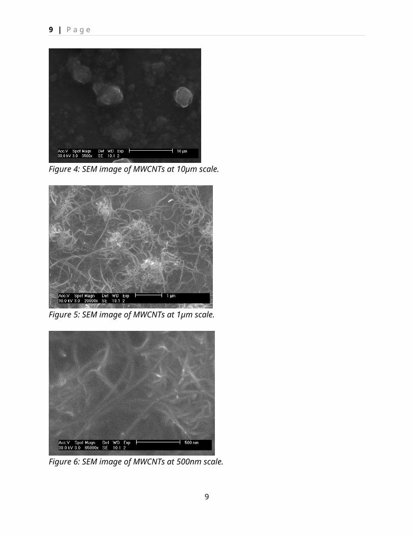
Figure 4: SEM image of MWCNTs at 10µm scale.

6

7 | P a g e

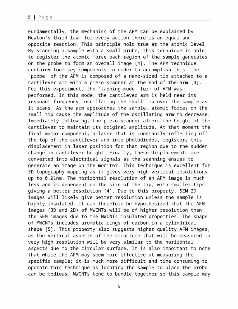
Figure 5: SEM image of MWCNTs at 1µm scale.

Figure 6: SEM image of MWCNTs at 500nm scale.

Figure 7: SEM image of MWCNTs at 200nm scale.Estimated Diameter (nm) ~60.9 nm

7

8 | P a g e

Estimated Length (µm) ~3.21 µmTable 1: Estimated diameter and length for MWCNTs measured by the SEM.

Figure 8: AFM cross-sectional measurements of MWCNTs (error).

Figure 9: AFM 2D image of MWCNTs (error).

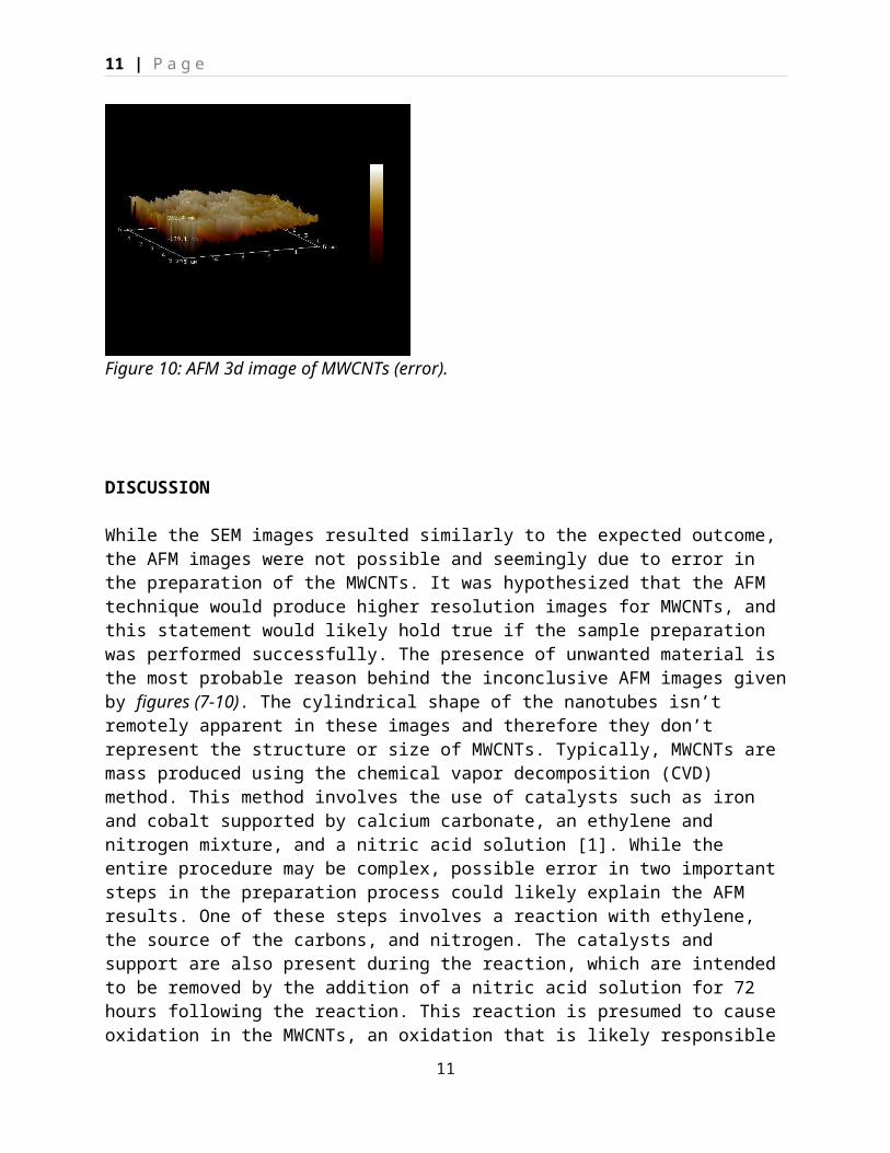
Figure 10: AFM 3d image of MWCNTs (error).

DISCUSSION

8

9 | P a g e

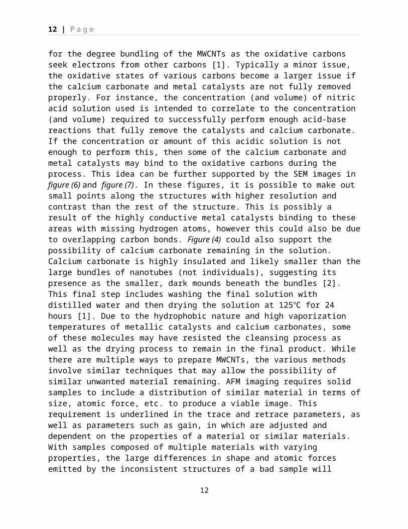
While the SEM images resulted similarly to the expected outcome, the AFM images were not possible and seemingly due to error in the preparation of the MWCNTs. It was hypothesized that the AFM technique would produce higher resolution images for MWCNTs, and this statement would likely hold true if the sample preparation was performed successfully. The presence of unwanted material is the most probable reason behind the inconclusive AFM images given by figures (7-10). The cylindrical shape of the nanotubes isn’t remotely apparent in these images and therefore they don’t represent the structure or size of MWCNTs. Typically, MWCNTs are mass produced using the chemical vapor decomposition (CVD) method. This method involves the use of catalysts such as iron and cobalt supported by calcium carbonate, an ethylene and nitrogen mixture, and a nitric acid solution [1]. While the entire procedure may be complex, possible error in two important steps in the preparation process could likely explain the AFM results. One of these steps involves a reaction with ethylene, the source of the carbons, and nitrogen. The catalysts and support are also present during the reaction, which are intended to be removed by the addition of a nitric acid solution for 72 hours following the reaction. This reaction is presumed to cause oxidation in the MWCNTs, an oxidation that is likely responsible for the degree bundling of the MWCNTs as the oxidative carbons seek electrons from other carbons [1]. Typically a minor issue, the oxidative states of various carbons become a larger issue if the calcium carbonate and metal catalysts are not fully removed properly. For instance, the concentration (and volume) of nitric acid solution used is intended to correlate to the concentration (and volume) required to successfully perform enough acid-base reactions that fully remove the catalysts and calcium carbonate. If the concentration or amount of this acidic solution is not enough to perform this, then some of the calcium carbonate and metal catalysts may bind to the oxidative carbons during the process. This idea can be further supported by the SEM images in figure (6) and figure (7). In these figures, it is possible to make out small points along the structures with higher resolution and contrast than the rest of the structure. This is possibly a result of the highly conductive metal catalysts binding to these areas with missing hydrogen atoms, however this could also be due to overlapping carbon bonds. Figure (4) could also support the possibility of calcium carbonate remaining in the solution. Calcium carbonate is highly insulated and likely smaller than the large bundles of nanotubes (not individuals), suggesting its presence as the smaller, dark mounds beneath the bundles [2]. This final step includes washing the final solution with distilled water and then drying the solution at 125oC for 24 hours [1]. Due to the hydrophobic nature and high vaporization temperatures of metallic catalysts and calcium carbonates, some of these molecules may have resisted the cleansing process as well as the drying process to remain in the final product. While there are multiple ways to prepare MWCNTs, the various methods involve similar techniques that may allow the possibility of similar unwanted material remaining. AFM imaging requires solid samples to include a distribution of similar material in terms of size, atomic force, etc. to produce a viable image. This requirement is underlined in the trace and retrace parameters, as well as parameters such as gain, in which are adjusted and dependent on the properties of a material or similar materials. With samples composed of multiple materials with varying properties, the large differences in shape and atomic forces emitted by the inconsistent structures of a bad sample will provide the impossibility for the parameters to align and generate a useful image. The larger material will typically “mask” the readings of the smaller material with less atomic force, and the overlapping of the two presents similar problems. The overall images from the AFM scans were given as seemingly random mountain-like shapes due to the scanning difficulty of the combined

9

10 | P a g e

material, resulting in the inconclusive AFM images. Overall, the calcium carbonate (or similar molecules dependent on preparation) theory is likely responsible for this imaging error due to its size of which is much larger and different than the individual MWCNTs themselves. It was therefore impossible to impose the appropriate parameters as the AFM would gradually scan the large calcium carbonate clumps and randomly read forces from overlapping nanotubes as they approached the probe.

The SEM images generated for this experiment were similar to their expectations. The SEM images were successful in terms of the expected properties of the MWCNTs such as conductivity and shape, as well as how they were suggested to interact with the SEM scanning process. Due to MWCNTs low conductivity, the sample was expected to decrease significantly in resolution as the SEM approached magnifications deeper along the nanometer scale. Figure (5) illustrates a high resolution image of the nanotubes at the micrometer scale, while figure (6) and figure (7) illustrate images of decreasing resolutions as the machine magnifies further down in nanometers as expected. The shape of the nanotubes were also as expected, however bundled together. This bundling formation, as well as the random areas of high resolution and clumped areas of low resolution, were due to the preparation error previously discussed. This error was minimized by the SEM technique as it allowed the undesirable areas to be ignored. The nanotubes from the images were further analyzed to give an estimated diameter of ~60.9 nm and an estimated length of ~3.21 µm, illustrated in table (1). These values were difficult to obtain due to the bundling formation and the expected low resolution images at high magnification. These values, however, hold similar measurements to the expected values given by various manufacturing companies such as US Research Nanomaterials, Inc [3]. According to this manufacturer, the outer diameters range from 30-60 nm while the lengths range from 1-10 µm [3]. The measurements from the experimental results are similar to these values and therefore can be considered accurate estimations. It was difficult to pinpoint the outer surfaces of the nanotubes in terms of their beginning and end, likely resulting in the slightly higher estimated diameter measurements. Overall, this technique generated the most accurate measurements for nanotubes between the two techniques with similar values to those expected.

CONCLUSION

In conclusion, this experiment was successful in generating a deeper understanding of the SEM and AFM microscopy techniques. The SEM images gave quite accurate results, while the AFM images resulted in error. Both of these results successfully provided information about the mechanisms of these techniques. The SEM images highlighted the impact that the conductivity of a sample has on its resolution, supported by the mechanism of the SEM’s electron-releasing requirements. The AFM images were unsuccessful, however they gave a deeper understanding of the overall AFM process and were successful in this regard. These inconclusive images further explained the AFM’s dependence on the materials present in a sample and how the atomic forces of these materials impact the overall readings. The large, varying differences in the size or atomic forces generated by the different materials of the sample were likely responsible for the error in the AFM images and gave a deeper understanding of the AFM mechanism. While the general mechanism of the AFM was explained prior to the experiment, it was interesting to see the degree at which this technique is sensitive to the different sizes of the materials present in a sample. With the SEM images supporting this variance in present materials, these results

10

11 | P a g e

indicated that both the SEM and AFM techniques were performed successfully and were impacted by this variance. These results also generated an understanding of the advantages and disadvantages of each machine. The SEM imaging technique was highly dependent on conductive material in order to give a high resolution image at the nanometer level, while this property has no effect on AFM imaging. In addition, SEM imaging was only able to generate 2D images while the AFM can produce 3D images. However, SEM imaging was performed much faster. The SEM technique allowed a quick scan of the sample at lower magnifications until areas were found that included the nanotubes, which were then magnified even further. The AFM technique required a trial-and-error approach in terms of finding the sample by adjusting the probe to different areas until the sample was found. The SEM technique was also far less sensitive to material property variance in the sample with the ability to scan and image without the different material properties impacting one another. The AFM results displayed that this technique is highly sensitive in this regard and is therefore undesirable for samples of this form. If the sample had been prepared successfully, the AFM results would have been able to generate a 3D representation of the sample with measurements such as height and cross-sectional area due to its high vertical resolution. These measurements are not possible with the SEM technique. By utilizing these techniques a deeper understanding of nanostructures such as MWCNTs was also obtained. The SEM images displayed the cylindrical shape and bundling tendency of nanostructures such as MWCNTs supported by processes in the nanotube’s preparation. The bi-products remaining in unsuccessful preparation, or non-pure MWCNT synthesis, were apparent in both of the imaging techniques. These bi-products gave a deeper understanding of the chemical mechanism in which these nanotubes are synthesized and the impact that small error has in preparation at the nanometer scale. Overall, the imaging results and the MWCNT properties simultaneously generated a deeper understanding of the other as this experiment progressed, resulting in a powerful learning experience in the area of nanotechnology.

REFERENCES

[1] Perez, Leon D., Manuel A. Zuluaga, Thein Kyu, James E. Mark, and Betty L. Lopez. "Preparation, Characterization, and Physical Properties of Multiwall Carbon Nanotube/elastomer Composites." Polym. Eng. Sci. Polymer Engineering & Science 49.5 (2009): 866-74. Web.

[2] Roy, Siddhartha. "Calcium Carbonate's Polymer Promise." Calcium Carbonate's Polymer Promise. Industrial Minerals, Nov. 2011. Web. 17 Sept. 2015.

[3] "Research Grade Large Inner Diameter Thin Multi-Wall Carbon Nanotubes, Purity: 90%, OD: 30-60nm, ID: 20-50nm." US Research Nanomaterials, Inc., n.d. Web. 17 Sept. 2015.

[4] Morgan, Timothy, and Radwan Al Faouri. Imaging NanoStructures. University of Arkansas, n.d. Web. 17 Sept. 2015.

[5] Mantena, Keerthi Varma. "ELECTRICAL AND MECHANICAL PROPERTIES OF MWCNT FILLED CONDUCTIVE ADHESIVES ON LEAD FREE SURFACE FINISHED PCB' S." UK Knowledge. University of Kentucky, 2009. Web. 17 Sept. 2015.

11

12 | P a g e

Lab Module 2: Synthesis and Optical Characterization of Au-Ag Nanoparticles

Jacob Feste

September 16, 2015

Group 2

Abstract

12

13 | P a g e

The purpose of this experiment was to synthesize hollow gold-silver (Au-Ag) nanoparticles and

characterize their optical properties. Initially, silver (Ag) nanoparticle synthesis was performed

via nucleation by reacting positively charged Ag+ ions with a sodium citrate reducing agent and a

poly(vinyl pyrrolidone) (PVP) capping agent to avoid oversaturation. The extinction peak for

these nanoparticles was around 427 nm. These Ag nanoparticles were then reacted with heat and

AuCl4- (aq) to generate the hollow Au-Ag nanoparticles by a galvanic replacement reaction. The

resulting TEM image included transparency and an expected reduction of overall nanoparticles;

supporting successful synthesis. The resulting UV absorbance readings illustrated a shifted

extinction peak more towards the NIR range (650-900 nm) and at around 495 nm with a wider

range of values. Also, light was scattered through these particles and these results suggest overall

successful synthesis and characterization.

Nomenclature

σ ext= Extinction cross-section (nm2).

ε m= Dielectric constant of the embedding medium.

ε i= Imaginary component of the metal dielectric function.

ε r= Real component of the metal dielectric function.

R = Radius (nm).

λ = Wavelength (nm)

13

14 | P a g e

Introduction

Metallic nanoparticles such as hollow Au-Ag nanoparticles have unique optical properties

associated with their size, especially when their sizes are smaller or similar to wavelengths of

light. Some metallic nanoparticles exhibit localized surface plasmons (LSP’s); of which may be

considered as oscillating charge densities within nanoparticles such as hollow Au-Ag

nanoparticles. The oscillation in LSP’s is a direct reflection of the electromagnetic fields

generated by incident light wavelengths, causing the charges in a nanoparticle to oscillate with

the electric field oscillation when a particle is smaller than a wavelength of light. The resonance

resulted in the LSP’s is termed localized surface plasma resonance (LSPR) and is due to the

LSP’s “resonating” nature within oscillating electric fields from incident light wavelengths [1].

This property creates an extinction peak that represents the scattering and absorbance of light

through the material, or the reduction (extinction) of the electromagnetic field [2]. The extinction

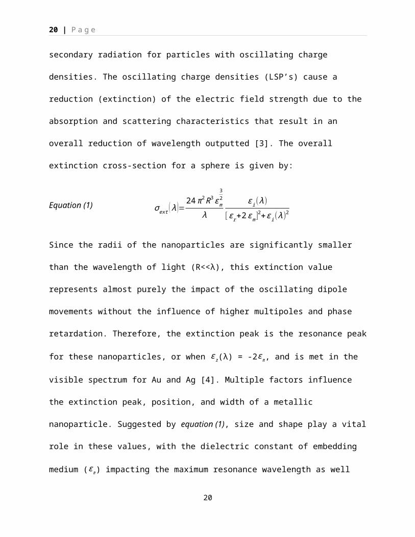
property is further explained by the Mie theory developed by Gustav Mie in 1908. Mie’s theory

suggests that the electromagnetic fields radiated and generated by incident light may be absorbed

or scattered as secondary radiation for particles with oscillating charge densities. The oscillating

charge densities (LSP’s) cause a reduction (extinction) of the electric field strength due to the

absorption and scattering characteristics that result in an overall reduction of wavelength

outputted [3]. The overall extinction cross-section for a sphere is given by:

Equation (1) σ ext ( λ )=24 π2 R3 ε m

32

λεi(λ)

[εr+2 ε m]2+εi(λ)2

Since the radii of the nanoparticles are significantly smaller than the wavelength of light (R<<λ),

this extinction value represents almost purely the impact of the oscillating dipole movements

without the influence of higher multipoles and phase retardation. Therefore, the extinction peak

14

15 | P a g e

is the resonance peak for these nanoparticles, or when ε r(λ) = -2ε m, and is met in the visible

spectrum for Au and Ag [4]. Multiple factors influence the extinction peak, position, and width

of a metallic nanoparticle. Suggested by equation (1), size and shape play a vital role in these

values, with the dielectric constant of embedding medium (ε m) impacting the maximum

resonance wavelength as well [2]. The properties listed above are present in both the Ag

nanoparticles and the hollow Au-Ag nanoparticles evaluated in this experiment. The Ag silver

nanoparticles can be expected to generate excitation peaks at smaller wavelengths than the

hollow Au-Ag nanoparticles due to the hollowing process involving a reduction in size. This is

represent by a larger value for the first fraction in equation (1) and therefore an overall larger

wavelength. While imaging techniques such as the TEM technique may be used to represent the

size of the nanoparticles, UV spectrometry may be used to determine the size distribution among

the nanoparticles in addition to absorption since the measured wavelengths are directly related to

their size (radius).

Generation of the hollow Au-Ag nanoparticles begins with the generation of the Ag

nanoparticle involved in the process. Silver particles are typically associated with a positive

charge. Reducing agents such as the sodium citrate used in this experiment may remove this

charge, reducing the Ag particles into single atoms. As the atoms are generated, the atomic

concentrations gradually increase until they reach a supersaturation level known as the critical

atomic threshold. Beyond this threshold, the Ag atoms are forced to self-nucleate, decreasing

concentrations until the threshold is no longer reached and the energy required to self-nucleate

becomes more than the energy required to join an existing nucleus. This process creates

“growth” around a nucleated Ag nanoparticles to give clusters of these nanoparticles. If the

maximum concentration of this threshold is reached, oversaturation will occur and synthesis will

15

16 | P a g e

not be successful. A poly(vinyl pyrrolidone) (PVP) capping agent is used to prevent this [2]. The

Ag nanoparticles can therefore be expected to be highly clustered. Following this process, the

hollow Au-Ag nanoparticles are assembled by the following galvanic replacement reaction:

Equation (2) 3Ag(s)+AuCl4- heat (aq)Au(s)+3Ag+(aq)+4Cl-(aq)

This spontaneous reaction proceeds due to the reduction potential of Au from AuCl4- being larger

than that of Ag from Ag+ [2]. Therefore, the Ag nanoparticles are gradually “hollowed out” as

the reaction takes place and the Au begins to gradually remove the Ag nanoparticles. Since there

is a larger concentration of Ag on the edges and corners of the Ag nanoparticle surfaces, the Au

particles are first generated in areas such as these. The reaction then proceeds internally to

promote the hollowing process because the Ag concentration is higher internally than on the

surface. Using too much AuCl4- could completely disassemble the silver nanoparticles until only

suspended gold nanoparticles remain, while using too little could leave most of the Ag

nanoparticles untouched. For this experiment, 1 ml of AuCl4- was used and is expected to give a

decent degree of hollowing. The 3 to 1 Ag to Au stoichiometry of the reaction also suggests an

overall reduction nanoparticles in the final product.

Procedure

Supplies

Balance with resolution 1 mg 100 mL and 50 mL 3-neck round bottom flasks Magnetic stir bars Condenser and glass stoppers Magnetic stir plate and heating mantle Centrifuge and appropriate centrifuge tubes Bath sonicator

16

17 | P a g e

Timer UV-Vis acrylic cuvettes Pasteur pipettes and bulbs Calibrated micropipette with appropriate tips Laser Pointer

Chemicals

Silver Nitrate (AgNO3) Disodium Citrate Dihydrate (Na3C6H5O7.2H2O) Poly(vinylpryrrolione), M.W. 55000 (PVP) Tetrachloroauric acid trihydrate (HAuCl4.3H2O) Copper sulfate pentahydrate (CuSO4.5H2O) 18 Mohm distilled water

Instrumentation

UV-Vis spectrophotometer Transmission electron microscope (TEM) Jeol 1400 model

Ag Nanoparticle Synthesis

1. Add 19 mL of H20 to a 100 mL flask with a stir bar

2. Add 0.4 mL of 115 mM AgNO3

3. Place the flask on a heating mantle

4. Heat the flask to a boil, immediately adding 1 mL PVP and 0.25 mL of 12 mM KCl

solution

5. Stopper the flask and boil for 10 minutes, adding 1 mL of 112 mM citrate solution after 2

minutes

6. Monitor and observe the reaction until it appears turbid

7. Upon turbidity, allow heating for 10 additional minutes

8. After this time, remove the flask from the heat and allow it to cool at room temperature

for 10 minutes.

17

18 | P a g e

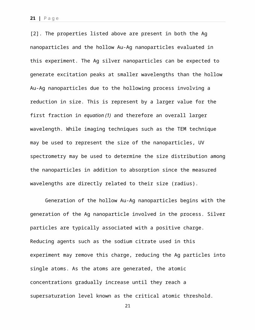
9. Purification begins by evenly distributing the nanoparticle solution into two 15 mL

centrifuge tubes and centrifuging at 6500 rpm for 15 minutes

10. Extract the supernatant with a Pasteur pipette

11. Add 5 mL H2O to each tube, sonicate to redisperse, and re-centrifuge at 6500 rpm for 20

minutes

12. Remove the supernatant and add 1.1 mL of H2O to each centrifuge tube and briefly

sonicate

13. Store the remaining product for further analysis

Hollow Au-Ag Nanoparticle Synthesis

1. Add 10 mL of H2O to a 50 mL flask with a stirring bar and allow it to heat for 10 minutes

2. Add 1 mL of PVP solution and 1 mL of the Ag nanoparticle suspension to the flask and

allow it to equilibrate for 2 minutes

3. Add 1 mL of 1 mM HAuCl4 dropwise to the solution at no faster than 0.5 mL/min

4. Store the remaining product for further analysis

UV-Vis Spectra Acquisition

1. Add 1.9 mL of H2O to a cuvette to obtain a blank (reference) spectrum

2. Add 0.1 mL of remaining Ag solution for a 20x dilution

3. Record the results

4. Repeat this process for 2 mL of Au-Ag solution in step 2 above

Absorption and Scattering

1. Shine a laser pointer through both solutions used for the UV readings and record any

observations

18

19 | P a g e

2. Repeat this process for a solution of 2 mL H2O and 2 mL of 100 mM CuSO4

TEM Imaging

1. Begin by dropping the nanoparticle suspension on a TEM grid and allow it to dry at room

temperature

2. Allow someone experienced with TEM to acquire the TEM images

Results

Figure 1: TEM image of Ag nanoparticles at 100 nm scale.

Figure 2: TEM image of Ag nanoparticles at 50 nm scale.

19

20 | P a g e

Figure 3: TEM image of hollow Au-Ag nanoparticles at 100 nm scale.

Figure 4: Final product of Ag nanoparticle suspension.

20

21 | P a g e

Figure 5: Final product of hollow Au-Ag nanoparticle suspension.

200 300 400 500 600 700 800 900 1000 11000

0.51

1.52

2.53

Ag Nanoparticles UV Absorbance Readings

Wavelength (nm)

Abso

rban

ce

Figure 6: UV Absorbance readings for the Ag nanoparticles.

200 300 400 500 600 700 800 900 1000 11000

0.20.40.60.8

1

Hollow Au-Ag Nanoparticles UV Absorbance Readings

Wavelength (nm)

Abso

rban

ce

Figure 7: UV Absorbance readings for the Au-Ag nanoparticles.

21

22 | P a g e

Discussion

The results listed above are similar to those expected and therefore suggest successful Ag and

Au-Ag nanoparticle synthesis. According to figures 1 and 2, the TEM images of the Ag

nanoparticles suggest diameters ranging from about 20-70 nm. These images also illustrate the

expected clustering involved in the nucleation and growth process. The UV absorbance results

seen in figure 6 can also be used to suggest similar diameters. According to Mie’s theory, the

estimated diameter of the Ag nanoparticles can be calculated by the following equation:

Equation (3) D=√(24.01+( λmax−385 )∗100)+4.9

Where D is the sphere’s diameter and λmax is the LSPR maximum [2]. With a λmax of around 427

nm, this value suggests diameters around 70 nm. The typical values for the diameters of Ag

nanoparticles range from about 10-100 nm [5]. Figure 4 also illustrates the final turbid coloring

of the Ag nanoparticle suspension as expected. This information suggests overall successful Ag

nanoparticle synthesis. The results also suggest successful Au-Ag nanoparticle synthesis. The

overall hollowing process, as well as the expected reduction in overall particles due to

stoichiometry, can be supported by the TEM image in figure 3. This image is much more

transparent than the TEM images for the Ag nanoparticles to suggest the successful hollowing

process. This image also displays unaltered relative sizes consistent with the Ag nanoparticles as

expected. The color of the final product in figure 5 is shown to be yellow and less turbid than the

gray Ag nanoparticles, also suggesting the coatings of Au and overall synthesis. According to the

UV absorbance readings seen in figure 7, the extinction peak was shifted more towards the NIR

range at around 495 nm. These readings also display a wider peak with lower absorbance values

compared to the Ag nanoparticle readings. As the hollowing is expected to shift the peak towards

22

23 | P a g e

the NIR range, these results suggest a successful reaction. In addition, the wider peak is

supported by the variability in the nanoparticles as the reaction proceeds; with some particles

becoming coated in Au and hollowed out at different rates than others. Finally, the lower

absorbance values also suggest increased transparency and hollowing. The addition of Au3+

solution was performed with different amounts for different groups during the experiment,

ranging from 0.5-2 mL.1 mL of this solution was added for our group. By analyzing the UV

absorbance results of the different groups, it is evident that the extinction peak shifts more

towards the NIR range with increased Au3+ addition. This is further supported by the addition of

2 mL of Au3+ solution giving peaks around 820 nm. Overall, these results suggest successful

hollow Au-Ag nanoparticle synthesis and characterization. The properties listed in the

introduction support these results with an insignificant degree of error for this experiment. In

conclusion, the Ag and hollow Ag-Au nanoparticles successfully synthesized in this experiment

provided a deeper understanding of the optical properties of such nanoparticles and their overall

dependence on size, structure, and composition.

References

[1] Hutter, E., and J. H. Fendler. "Exploitation of Localized Surface Plasmon Resonance." Adv. Mater. Advanced Materials 16.19 (2004): 1685-706. Web.[2] Chin, Jingyi. "Synthesis of Hollow Gold-Silver Nanoparticles and Investigation of Their Optical Properties." University of Arkansas(2015): n. pag. Web.[3] Wriedt, Thomas. "Mie Theory: A Review." The Mie Theory Springer Series in Optical Sciences (2012): 53-71. Web.[4] Parang, Z., A. Keshavarz, S. Farahi, S.m. Elahi, M. Ghoranneviss, and S. Parhoodeh. "Fluorescence Emission Spectra of Silver and Silver/cobalt Nanoparticles." Scientia Iranica 19.3 (2012): 943-47. Web.[5] Oldenburg, Stephen J. "Silver Nanoparticles: Properties and Applications."Sigma-Aldrich. N.p., n.d. Web. 30 Sept. 2015.

23

24 | P a g e

Lab 10: Fluorescence Microscopy

Jacob Feste

010617389

4/20/15

Objective

The objective of this experiment is to transfect NIH-3T3 mammalian cells with an adenoviral vector carrying the gene for Green Fluorescent Protein (GFP), and to verify this transfection visually using fluorescence microscopy. The transfection process will occur biologically by simply mixing the NIH-3T3 cells with a diluted form of the adenovirus. The adenoviral vector is originally obtained by the direct transfection of cells from a 293 cell line with the GFP gene. After a few days, the supernatant of these cells is collected as a diluted form of the adenovirus and is used for the 200 MOI viral media. This media is added to the NIH-3T3 cell culture with the mixture incubated to allow the natural transfection of the viral DNA to the cells. The results will be identified using fluorescence microscopy with DAPI. Fluorescence microscopy applies light at specific wavelengths, or color, to the specimen and excites its photons, causing them to absorb and re-emit light at different wavelengths. The differences in wavelength, or color, are detected by the microscope to give a visual representation of the excited regions of the specimen. In order to detect the degree of GFP gene transfection, DAPI will also be applied to the cells to indicate the presence of each cell. GFP emits a bright green color when subject to specific wavelengths, while DAPI localizes at the nuclei to emit a blue color when subject to specific wavelengths. Therefore, successful fluorescence microscopy results should include a blue region for each cell indicating their nuclei. In addition, successful transfection results should include bright green regions, indicating that the cells had successfully integrated the GFP coding DNA into their own.

Materials

1. NIH-3T3 mammalian cells2. 120µL adenovirus3. PBS (1X) 4. PFA (Paraformaldehyde) 5. Prolong mounting medium 6. DAPI 7. Disposable pipette 8. Fine point tweezer 9. PDMS coated cover slips 10. Glass slides 11. 6 well-plates 12. Fluorescence microscopy

24

25 | P a g e

Procedure

Adenoviral Transfection:

1. Place PDMS coated coverslips into 6 well-plates 2. Add 5 ml of 3T3 cell cultures (106 = number of cells) to each well plate with PDMS

coated coverslips (Cells will attach to the coverslips) 3. Prepare 200 MOI viral media by adding 20µL adenovirus (1010 pfu/ml) to each well-

plate with cell cultures 4. Mix the solution by tilting the well-plate up and down 5. Incubate it for 48 hours

Sample Fixation and DAPI staining:

1. Fixation and staining are performed after 48h incubation period. 2. Prepare PFA (Paraformaldehyde) solution by diluting it with PBS (Dilution factor is 1:4) 2.

After 48h, aspirate the viral media from 6 well-plates, and wash the samples with PBS (X 3 times)

3. Add 3 ml of the PFA solution to each well, and wait for 15 min. 4. After 15 min, aspirate the PFA solution, and wash the samples with PBS (x3) (wait for 5

min each time) 5. Samples are ready for DAPI staining. 6. Dilute DAPI by PBS (Dilution factor is 1:200). Add 200µL diluted DAPI solution to the

petri dish. 7. Take the coverslip, flip it over (the surface attached with cells will touch to the DAPI

solution), and place it into the DAPI solution. 8. Incubate the cells for 1 h. 9. After 1h, take the coverslip from the petri dish, flip it over (the surface attached with

cells will look up), and place it into the 6 well-plates for washing. 10. Wash the samples with PBS (x3) (wait for 5 min each time) in the 6-well plates. 11. Add one drop of Prolong (a liquid mountant) on the glass slide (Be careful!!- Do not

make bubbles!) 12. Take the coverslip from the 6 well-plates, flip it over again (take excess PBS from the

coverslip by touching the coverslip to the kimwipes), and place it onto the Prolong drop slowly (Be careful!!- Do not make bubbles!)

13. Leave the glass slide with cover slip for drying for at least 3 hrs. 14. It is ready to use for fluorescence microscopy.

Results

The results included a fluorescence microscopy image of the NIH-3T3 cells with blue regions for each cell and a noticeable degree of bright green regions within the cells.

25

26 | P a g e

Discussion and Conclusion

The objective of this experiment was to successfully transfect NIH-3T3 mammalian cells with the GFP gene, while successfully performing fluorescence microscopy to visual the transfection. Our results included a fluorescence microscopy image of NIH-3T3 cells with blue regions at their nuclei and bright green regions present throughout. Therefore, our results indicate that the objective was met successfully. The use of DAPI with fluorescence microscopy in order to indicate the nuclei of the cell culture was successful as our results illustrate emitted wavelengths that generated a blue color at each nuclei. Transfection of the GFP gene via adenoviral vectors can also be considered successful by our results. The results generated regions of bright green wavelengths, of which are emitted by GFP proteins. The adenoviral vectors containing the GFP genes were removed prior to fluorescence, leaving the cells as the only possible GFP source. Therefore, these bright green regions were produced by the GFP proteins in the cells and indicate that the cells were successfully transfected to include GFP production. While fluorescence microscopy was successfully able to confirm transfection, other methods can also be performed to determine successful transfection. Southern blotting is a very effective tool for analyzing DNA. The southern blotting process begins by digesting the tested DNA with restriction enzymes and separating it by molecular weight using gel electrophoresis. It is also incubated with NaOH to denature and separate the strands. The separated components are transferred, with the same pattern of separation, to a membrane consisting of special blotting paper. Altogether, this process separates the DNA of the tested cells while maintaining an environment that allows binding to other molecules. The process then applies a probe consisting of single strands of the DNA of whose presence in the tested cells is being determined. The probe would include the GFP gene for this experiment and is labeled either radioactively or enzyme-linked. Incubation of the probe with the tested DNA allows the probe DNA to bind with its complimentary base pairs if they are present. Finally, the presence of the desired DNA is indicated by X-Ray analysis. For enzyme-linked labeling the addition of colorless substrate, of which the enzyme linked to the probe converts to a colored product, exposes the X-Ray film while radioactively labeling directly exposes the X-Ray film. The presence of a specific DNA is therefore indicated by X-Ray analysis. This method can be performed on the DNA of the NIH-3T3 cells with the GFP gene as a probe in order to determine its successful transfection. The quality of the fluorescence microscopy image of our results was decent with enough quality to accurately illustrate the results. However, the quality could certainly improve to improve accuracy. Since only the nuclei were stained, it made it difficult to visualize the remainder of the cell. Dyes such as Texas Red could have been used to image the cytoskeleton of each cell as well, allowing the visualization of each cell’s interior area. Other components, such as mitochondria, also could’ve been visualized with dyes such as Alexafluor 488. The increasing visualization of each cell’s elements allows the increasingly accurate determination of areas such as how many GFP proteins reside in each cell, the size of GFP proteins in respect to other components, and which cells were transfected successfully. Visualization of the components of the cell improve quality and accuracy, of which could also be improved by more specific wavelength applications and higher resolution microscopes. In conclusion the NIH-3T3 cells were successfully transfected with the GFP gene, of which was successfully supported by fluorescence microscopy.

26

27 | P a g e

27