EXAMPLES AND APPLICATIONS OF NONCOMMUTATIVE GEOMETRY …jmr/BuenosAires/NCGexamples.pdf ·...

EXAMPLES AND APPLICATIONS OF NONCOMMUTATIVE

GEOMETRY AND K-THEORY

JONATHAN ROSENBERG

Abstract. These are informal notes from my course at the 3era Escuela deInvierno Luis Santalo-CIMPA Research School on Topics in NoncommutativeGeometry. Feedback, especially from participants at the course, is very wel-come.

The course basically is divided into two (related) sections. Lectures 1–3deal with Kasparov’s KK-theory and some of its applications. Lectures 4–5deal with one of the most fundamental examples in noncommutative geometry,the noncommuative 2-torus.

Contents

Lecture 1. Introduction to Kasparov’s KK-theory 31.1. Why KK? 31.2. Kasparov’s original definition 41.3. Connections and the product 71.4. Cuntz’s approach 81.5. Higson’s approach 9Lecture 2. K-theory and KK-theory of crossed products 112.1. Equivariant Kasparov theory 112.2. Basic properties of crossed products 122.3. The dual action and Takai duality 132.4. Connes’ “Thom isomorphism” 132.5. The Pimsner-Voiculescu Theorem 162.6. The Baum-Connes Conjecture 162.7. The approach of Meyer and Nest 18Lecture 3. The universal coefficient theorem for KK and some of its

applications 193.1. Introduction to the UCT 193.2. The proof of Rosenberg and Schochet 193.3. The equivariant case 203.4. The categorical approach 203.5. The homotopy-theoretic approach 223.6. Topological applications 223.7. Applications to C∗-algebras 23

Date: 2010.2010 Mathematics Subject Classification. Primary 46L85; Secondary 19-02 46L87 19K35.Preparation of these lectures was partially supported by NSF grant DMS-0805003 and DMS-

1041576. The author thanks the members of the GNC Group at Buenos Aires, and especiallyGuillermo Cortinas, for their excellent organization of the Winter School.

1

2 JONATHAN ROSENBERG

Lecture 4. A fundamental example in noncommutative geometry:topology and geometry of the irrational rotation algebra 24

4.1. Basic facts about Aθ 244.2. Basic facts about A∞

θ 264.3. Geometry of vector bundles 274.4. Miscellaneous other facts about Aθ 28Lecture 5. Applications of the irrational rotation algebra in number

theory and physics 295.1. Applications to number theory 295.2. Applications to physics 29References 30

APPLICATIONS OF NONCOMMUTATIVE GEOMETRY 3

Lecture 1. Introduction to Kasparov’s KK-theory

1.1. Why KK? KK-theory is a bivariant version of topological K-theory, definedfor C∗-algebras, with or without a group action. It can be defined for either realor complex algebras, but in these notes we will stick to complex algebras for sim-plicity. Thus if A and B are complex C∗-algebras, subject to a minor technicalrequirement (that B be σ-unital, which is certainly the case if it is either uni-tal or separable), an abelian group KK(A,B) is defined, with the property thatKK(C, B) = K(B) = K0(B) if the first algebra A is just the scalars. (For the basicproperties of K0, I refer you to the courses by Reich and Karoubi.) The theorywas defined by Gennadi Kasparov in a remarkable series of papers: [33, 34, 35].However, the definition at first seems highly technical and unmotivated, so it’sworth first seeing where the theory comes from and why one might be interestedin it. For purposes of this introduction, we will only be concerned with the casewhere A and B are commutative. Thus A = C0(X) and B = C0(Y ), where X andY are locally compact Hausdorff spaces. We will abbreviate KK(C0(X), C0(Y ))to KK(X,Y ). It is worth pointing out that the study of KK(X,Y ) (withoutconsidering KK(A,B) more generally) is already highly nontrivial, and encom-passes most of the features of the general theory. Note that we expect to haveKK(C, C0(Y )) = KK(pt, Y ) = K(Y ), the K-theory of Y with compact support.Recall that this is the Grothendieck group of complexes of vector bundles that areexact off a compact set. It’s actually enough to take complexes of length 2, soan element of K(Y ) is represented by a pair of vector bundles V and V ′ over Y ,

together with a morphism of vector bundles Vϕ−→ V ′ that is an isomorphism off

a compact set. Alternatively, K(Y ) can be identified with the reduced K-theory

K(Y+) of the one-point compactification Y+ of Y .A good place to start in trying to understand KK is Atiyah’s paper [4] on

the Bott periodicity theorem. Bott periodicity, or more generally, the Thom iso-morphism theorem for a complex vector bundle, asserts that if p : E → X isa complex vector bundle (more generally, one could take an even-dimensionalreal vector bundle with a spinc structure), then there is a natural isomorphismβE : K(X) → K(E), called the Thom isomorphism in K-theory. In the specialcase where X = pt, E is just Cn for some n, and we are asserting that there is

a natural isomorphism Z = K(pt) → K(Cn) = K(R2n) = K(S2n), the Bott pe-riodicity map. The map βE can be described by the formula βE(a) = p∗(a) · τE .Here p∗(a) is the pull-back of a ∈ K(X) to E. Since a had compact support, p∗(a)has compact support in the base direction of E, but is constant on fibers of p, soit certainly does not have compact support in the fiber direction. However, wecan multiply it by the Thom class τE , which does have compact support along thefibers, and the product will have compact support in both directions, and will thusgive a class in K(E) (remember that since E is necessarily noncompact, assumingn > 0, we need to use K-theory with compact support). The Thom class τE , inturn, can be described [59, §3] as an explicit complex

∧• p∗E over E. The vectorbundles in this complex are the exterior powers of E pulled back from X to E, and

the map at a point e ∈ Ex from∧j

Ex to∧j+1

Ex is simply exterior product withe. This complex has compact support in the fiber directions since it is exact off thezero-section of E. (If e 6= 0, then the kernel of e∧ is spanned by products e∧ω.)


So far this is all simple vector bundle theory and KK is not needed. But it comesin at the next step. How do we prove that βE is an isomorphism? The simplestway would be to construct an inverse map αE : K(E) → K(X). But there is noeasy way to describe such a map using topology alone. As Atiyah recognized, theeasiest way to construct αE uses elliptic operators, in fact the family of Dolbeaultoperators along the fibers of E. Thus whether we like it or not, some analysis comesin at this stage. In more modern language, what we really want is the class αEin KK(E,X) corresponding to this family of operators, and the verification of theThom isomorphism theorem is a Kasparov product calculation, the fact that αE is aKK inverse to the class βE ∈ KK(X,E) described (in slightly other terms) before.Atiyah also noticed [4] that it’s really just enough (because of certain identitiesabout products) to prove that αE is a one-way inverse to βE , or in other words, inthe language of Kasparov theory, that βE ⊗E αE = 1X . This comes down to anindex calculation, which because of naturality comes down to the single calculationβ ⊗C α = 1 ∈ KK(pt, pt) when X is a point and E = C, which amounts to theRiemann-Roch theorem for CP1.

What then is KK(X,Y ) when X and Y are locally compact spaces? An elementof KK(X,Y ) defines a map of K-groups K(X) → K(Y ), but is more than this;it is in effect a natural family of maps of K-groups K(X × Z) → K(Y × Z) forarbitrary Z. Naturality of course means that one gets a natural transformation offunctors, from Z 7→ K(X × Z) to Z 7→ K(Y × Z). (Nigel Higson has pointed outthat one can use this in reverse to define KK(X,Y ) as a natural family of mapsof K-groups K(X × Z) → K(Y × Z) for arbitrary Z. The reason why this workswill be explained in Lecture 3 in this series.) In particular, since KK(X × Rj)can be identified with K−j(X), an element of KK(X,Y ) defines a graded map ofK-groups Kj(X) → Kj(Y ), at least for j ≤ 0 (but then for arbitrary j becauseof Bott periodicity). The example of Atiyah’s class αE ∈ KK(E,X), based ona family of elliptic operators over E parametrized by X , shows that one gets anelement of the bivariant K-group KK(X,Y ) from a family of elliptic operatorsover X parametrized by Y . The element that one gets should be invariant underhomotopies of such operators. Hence Kasparov’s definition of KK(A,B) is basedon a notion of homotopy classes of generalized elliptic operators for the first algebraA, “parametrized” by the second algebra B (and thus commuting with a B-modulestructure).

1.2. Kasparov’s original definition. As indicated above in Section 1.1, an ele-ment of KK(A,B) is roughly speaking supposed to be a homotopy class of familiesof elliptic pseudodifferential operators over A parametrized by B. For technicalreasons, it’s convenient to work with self-adjoint bounded operators1, but it’s well-known that the most interesting elliptic operators send sections of one vector bundleto sections of another. The way to get around this is to take our operators to beself-adjoint, but odd with respect to a grading, i.e., of the form

(1.1) T = T ∗ =

(0 F ∗

F 0

).

1Often we want to apply the theory to self-adjoint differential operators D, which are never

bounded on L2 spaces. The trick is to replace D by D(1 + D2)−12 , which has the same index

theory as D and is bounded.


The operator F here really does act between different spaces, but T , built fromF and F ∗, is self-adjoint, making it easier to work with. Then we need variousconditions on T that correspond to the terms “elliptic,” “pseudodifferential,” and“parametrized by B.” So this boils down to the following. A class in KK(A,B) isrepresented by a Kasparov A-B-bimodule, that is, a Z/2-graded (right) Hilbert B-module H = H0⊕H1, together with a B-linear operator T ∈ L(H) of the form (1.1),and a (grading-preserving) ∗-representation φ of A on H, subject to the conditionsthat φ(a)(T 2 − 1) ∈ K(H) and [φ(a), T ] ∈ K(H) for all a ∈ A. These conditionsrequire a few comments. The condition that φ(a)(T 2 − 1) ∈ K(H) is “ellipticity”and the condition that [φ(a), T ] ∈ K(H) is “pseudolocality.” If B = C, a HilbertB-module is just a Hilbert space, L(H) is the set of bounded linear operators onH, and K is the set of compact operators on H. If B = C0(Y ), a Hilbert B-module is equivalent to a continuous field of Hilbert spaces over Y . In this case,K(H) is the associated set of continuous fields of compact operators, while L(H)consists of continuous fields (continuity taken in the strong-∗ operator topology) ofbounded Hilbert space operators. If X is another locally compact space, then itis easy to see that Kasparov’s conditions are an abstraction of a continuous familyof elliptic pseudolocal Hilbert space operators over X , parametrized by Y . Finally,if B is arbitrary, a Hilbert B-module means a right B-module equipped with aB-valued inner product 〈 , 〉B, right B-linear in the second variable, satisfying〈ξ, η〉B = 〈η, ξ〉∗B and 〈ξ, ξ〉B ≥ 0 (in the sense of self-adjoint elements of B),with equality only if ξ = 0. Such an inner product gives rise to a norm on H:

‖ξ‖ = ‖〈ξ, ξ〉B‖1/2B , and we require H to be complete with respect to this norm.

Given a Hilbert B-module H, there are two special C∗-algebras associated to it.The first, called L(H), consists of bounded B-linear operators a on H, admittingan adjoint a∗ with the usual property that 〈aξ, η〉B = 〈ξ, a∗η〉B for all ξ, η ∈ H.Unlike the case where B = C, existence of an adjoint is not automatic, so it must beexplicitly assumed. Then inside L(H) is the ideal of B-compact operators. This isthe closed linear span of the “rank-one operators” Tξ,η defined by Tξ,η(ν) = ξ〈η, ν〉B .Note that

〈Tξ,η(ν), ω〉B = 〈ξ〈η, ν〉B , ω〉B = 〈ω, ξ〈η, ν〉B〉∗B

= (〈ω, ξ〉B〈η, ν〉B)∗

= 〈η, ν〉∗B〈ω, ξ〉∗B

= 〈ν, η〉B〈ξ, ω〉B = 〈ν, η〈ξ, ω〉B〉B

= 〈ν, Tη,ξ(ω)〉B ,

so that T ∗ξ,η = Tη,ξ. It is also obvious that if a ∈ L(H), then aTξ,η = Taξ,η, while

Tξ,ηa = T ∗η,ξ

(a∗

)∗=

(a∗Tη,ξ

)∗= T ∗

a∗η,ξ = Tξ,a∗η, so these rank-one operators

generate an ideal in L(H), which is just the usual ideal of compact operators incase B = C. For more on Hilbert C∗-modules and the C∗-algebras acting on them,see [40] or [46, Ch. 2].

The simplest kind of Kasparov bimodule is associated to a homomorphismφ : A → B. In this case, we simply take H = H0 = B, viewed as a right B-module, with the B-valued inner product 〈b1, b2〉B = b∗1b2, and take H1 = 0 andT = 0. In this case, L(H) = M(B) (the multiplier algebra of B, the largest C∗-algebra containing B as an essential ideal), and K(H) = B. So φ maps A intoK(H), and even though T = 0, the condition that φ(a)(T 2 − 1) ∈ K(H) is satisfiedfor any a ∈ A.


One special case which is especially important is the case where A = B and φis the identity map. The above construction then yields a distinguished element1A ∈ KK(A,A), which will play an important role later.

In applications to index theory, Kasparov A-B-bimodules typically arise fromelliptic (or hypoelliptic) pseudodifferential operators. However, there are otherways to generate Kasparov bimodules which we will discuss in Section 1.4 below.

So far we have explained what the cycles are for KK-theory, but not the equiv-alence relation that determines when two such cycles give the same KK-element.First of all, there is a natural associative addition on Kasparov bimodules, ob-tained by taking the direct sum of Hilbert B-modules and the block direct sumof homomorphisms and operators. Then we divide out by the equivalence relationgenerated by addition of degenerate Kasparov bimodules (those for which for alla ∈ A, φ(a)(T 2 −1) = 0 and [φ(a), T ] = 0) and by homotopy. (A homotopy of Kas-parov A-B-bimodules is just a Kasparov A-C([0, 1], B)-bimodule.) Then it turnsout that the resulting semigroup KK(A,B) is actually an abelian group, with in-version given by reversing the grading, i.e., reversing the roles of H0 and H1, andinterchanging F and F ∗. Actually, it was not really necessary to divide out bydegenerate bimodules, since if (H, φ, T ) is degenerate, then (C0((0, 1],H) (alongwith the action of A and the operator which are given by φ and T at each point of(0, 1]) is a homotopy from (H, φ, T ) to the 0-module.

An interesting exercise is to consider what happens when A = C and B is a unitalC∗-algebra. Then if H0 and H1 are finitely generated projective (right) B-modulesand we take T = 0 and φ to be the usual action of C by scalar multiplication,we get a Kasparov C-B-bimodule corresponding to the element [H0] − [H1] ofK0(B). With some work one can show that this gives an isomorphism betweenthe Grothendieck group K0(B) of usual K-theory and KK(C, B). By consideringwhat happens when one adjoins a unit, one can then show that there is still anatural isomorphism between K0(B) and KK(C, B), even if B is nonunital.

Another important special case is when A and B are Morita equivalent in thesense of Rieffel [47, 50] — see [46] for a very good textbook treatment. That meanswe have an A-B-bimodule X with the following special properties:

(1) X is a right Hilbert B-module and a left Hilbert A-module.(2) The left action of A is by bounded adjointable operators for the B-valued

inner product, and the right action ofB is by bounded adjointable operatorsfor the A-valued inner product.

(3) The A- and B-valued inner products on X are compatible in the sense thatif ξ, η, ν ∈ X , then A〈ξ, η〉ν = ξ〈η, ν〉B .

(4) The inner products are “full,” in the sense that the image of A〈 , 〉 isdense in A, and the image of 〈 , 〉B is dense in B.

Under these circumstances, X defines classes in [X ] ∈ KK(A,B) and [X] ∈KK(B,A) which are inverses to each other (with respect to the product discussedbelow in Section 1.3). Thus as far as KK-theory is concerned, A and B are es-

sentially equivalent. The construction of [X ] and of [X ] is fairly straightforward;for example, to construct [X ], take H0 = X (viewed as a right Hilbert B-module),H1 = 0, and T = 0, and let φ : A → L(H) be the left action of A (which factorsthrough L(H) by axiom (2)). By axiom (4) (which is really the key property), anyelement of A can be approximated by linear combinations of inner products A〈ξ, η〉.


For such an inner product, we have

φ(A〈ξ, η〉)ν = ξ〈η, ν〉B = Tξ,η(ν),

so the action of A on H is by operators in K(H), which is what is needed for theconditions for a Kasparov bimodule.

The prototype example of a Morita equivalence has A = C, B = K(H) (weusually drop the H and just write K if the Hilbert space is infinite-dimensional andseparable), and X = H, with the B-valued inner product taking a pair of vectors inH to the corresponding rank-one operator. Thus from the point of KK-theory, C

and K are essentially indistinguishable, and so are B and B ⊗K for any B. Thereis a converse [10]; separable C∗-algebras A and B are Morita equivalent if and onlyif A ⊗ K and B ⊗ K are isomorphic. (This condition, called stable isomorphism,is obviously satisfied by B and B ⊗ K, since (B ⊗ K) ⊗ K ∼= B ⊗ (K ⊗ K) ∼=B ⊗K.) However, a Morita equivalence between A and B leads directly to a KK-equivalence, but not directly to an isomorphism A ⊗ K ∼= B ⊗ K (which requiressome arbitrary choices).

The most readable references for the material of this section are the book byBlackadar [6], Chapter VIII, and the “primer” of Higson [29].

1.3. Connections and the product. The hardest aspect of Kasparov’s approachto KK is to prove that there is a well-defined, functorial, bilinear, and associativeproduct ⊗B : KK(A,B) × KK(B,C) → KK(A,C). There is also an external

product ⊠ : KK(A,B) ×KK(C,D) → KK(A⊗ C,B ⊗D), where ⊗ denotes thecompleted tensor product. (For our purposes, the minimal or spatial C∗-tensorproduct will suffice.) The external product is actually built from the usual productusing an operation called dilation (external product with 1). We can dilate a classa ∈ KK(A,B) to a class a⊠ 1C ∈ KK(A⊗ C,B ⊗ C), by taking a representative(H, φ, T ) for a to the bimodule (H ⊗ C, φ ⊗ 1C , T ⊗ 1). Similarly, we can dilate aclass b ∈ KK(C,D) (on the other side) to a class 1B ⊠ b ∈ KK(B ⊗ C,B ⊗ D).Then

a⊠ b = (a⊠ 1C) ⊗B⊗C (1B ⊠ b) ∈ KK(A⊗ C,B ⊗D),

and one can check that this is the same as what one gets by computing in the otherorder as (1A ⊠ b) ⊗A⊗D (a⊠ 1D).

The Kasparov products, as they are called, encompass the usual cup and capproducts relating K-theory and K-homology. For example, the cup product inordinary topological K-theory for a compact space X , ∪ : K(X)×K(X) → K(X),is a composite of two products. Given a ∈ K(X) = KK(C, C(X)) and b ∈ K(X) =KK(C, C(X)), we first form the external product a⊠ b ∈ KK(C, C(X)⊗C(X)) =KK(C, C(X ×X)). Then we have

a ∪ b = (a⊠ b) ⊗C(X×X) ∆,

where ∆ ∈ KK(C(X × X), C(X)) is the class of the homomorphism defined byrestriction of functions on X ×X to the diagonal copy of X .

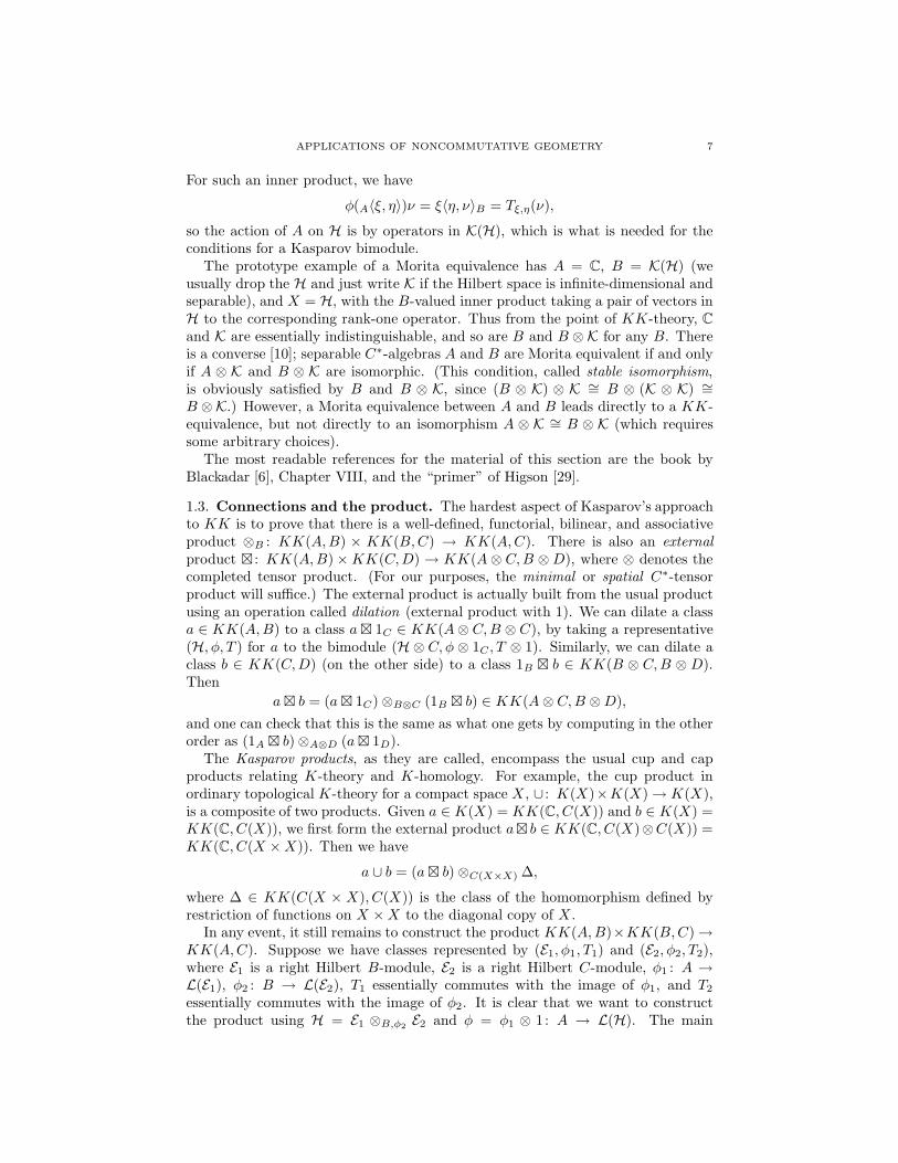
In any event, it still remains to construct the product KK(A,B)×KK(B,C) →KK(A,C). Suppose we have classes represented by (E1, φ1, T1) and (E2, φ2, T2),where E1 is a right Hilbert B-module, E2 is a right Hilbert C-module, φ1 : A →L(E1), φ2 : B → L(E2), T1 essentially commutes with the image of φ1, and T2

essentially commutes with the image of φ2. It is clear that we want to constructthe product using H = E1 ⊗B,φ2

E2 and φ = φ1 ⊗ 1: A → L(H). The main


difficulty is getting the correct operator T . In fact there is no canonical choice;the choice is only unique up to homotopy. The most convenient method of doingthe construction seems to be using the notion of a connection due to Connes andSkandalis [13], nicely explained in [6, §18] or [61].

To motivate this, let’s just consider a simple example that comes up in indextheory, the construction of an “elliptic operator with coefficients in a vector bundle.”Let T be an elliptic operator on a compact manifold M , which we take to be abounded operator of the form (1.1) (acting on a Z/2-graded Hilbert space H), andlet E be a complex vector bundle over M . Often we want to form TE , the sameoperator with coefficients in the vector bundle E. This is actually a special caseof the Kasparov product. The sections Γ(M,E) are a finitely generated projectiveC(M)-module E ; since C(M) is commutative, we can regard this as a C(M)-C(M)-bimodule, with the same action on the left and on the right. Then E (concentratedentirely in degree 0, together with the 0-operator), defines a KK-class [[E]] ∈KK(M,M), while T defines a class [T ] in KK(M, pt). Note that forgetting theleft C(M)-action on E is the same as composing with inclusion of the scalars C →C(M) to get from [[E]] a class [E] ∈ KK(pt,M) = K(M), which is the usualK-theory class of E. The class of the operator TE will be the Kasparov product[[E]] ⊗M [T ] ∈ KK(M, pt). Defining the operator, however, requires a choice ofconnection on the bundle E. One way to get this is to embed E as a direct summandin a trivial bundle M × Cn. Then orthogonal projection onto E is given by a self-adjoint projection p ∈ C(M,Mn(C)). We can certainly form T ⊗ 1 acting onH ⊗ Cn, on which we have an obvious action of C(M) ⊗Mn(C), but there is noreason why T ⊗ 1 and p should commute, so there is no “natural” cut-down of Tto E. Thus we simply take the compression T ′ = p(T ⊗ 1)p acting on H′ = pHwith the obvious action φ′ of C(M). Since T commutes with the action of C(M)up to compact operators, the commutator [p, T ⊗ 1] is also compact, so T ′ satisfiesthe requirements that (T ′)2 − 1 ∈ K(H′) and [φ′(f), T ′] ∈ K(H′). Its Kasparovclass is well-defined, even though there is great freedom in choosing the operator(corresponding to the freedom to embed E in a trivial bundle in many differentways). (When n is large enough, all vector bundle embeddings of E into M × Cn

are isotopic, and thus the operators obtained by the above construction will behomotopic in a way preserving the Kasparov requirements.)

1.4. Cuntz’s approach. Joachim Cuntz noticed in [17] that all Kasparov bimod-ules can be taken to come from the basic notion of a quasihomomorphism betweenC∗-algebras A and B. A quasihomomorphism A ⇉ D D B is roughly speaking aformal difference of two homomorphisms f± : A→ D, neither of which maps into Bitself, but which agree modulo an ideal isomorphic to B. Thus a 7→ f+(a) − f−(a)is a linear map A→ B. Suppose for simplicity (one can always reduce to this case)that D/B ∼= A, so that f± are two splittings for an extension

0 → B → D → A→ 0.

Then for any split-exact functor F from C∗-algebras to abelian groups (meaningit sends split extensions to short exact sequences — an example would be F (A) =K(A⊗ C) for some coefficient algebra C), we get an exact sequence

0 // F (B) // F (D) // F (A) //

(f+)∗rr

(f−)∗

ll 0.


Thus (f+)∗ − (f−)∗ gives a well-defined homomorphism F (A) → F (B), which wemight well imagine should come from a class in KK(A,B). (Think about Section1.1, where we mentioned Higson’s idea of defining KK(X,Y ) in terms of naturaltransformations of functors, from Z 7→ K(X × Z) to Z 7→ K(Y × Z). We willcertainly get such a natural transformation from a quasihomomorphism C0(X)⇉D D C0(Y )⊗K, since C0(Y )⊗K and Y have the sameK-theory.) And indeed, givena quasihomomorphism as above, we get a Kasparov A-B-bimodule, with B ⊕B asthe Hilbert B-module (with the obvious grading), with φ : A→ L(B ⊕ B) definedby (

f+ 00 f−

), and T =

(0 11 0

).

The “almost commutation” relation is[(f+(a) 0

0 f−(a)

),

(0 11 0

)]=

(0 f+(a) − f−(a)

f−(a) − f+(a) 0

)∈ K(B ⊕B),

since K(B⊕B) = M2(B). In the other direction, given a Kasparov A-B-bimodule,one can add on a degenerate bimodule and do a homotopy to reduce it to somethingroughly of this form, showing that all of KK(A,B) comes from quasihomomor-phisms (see [6, §17.6]).

The quasihomomorphism approach to KK makes it possible to define KK(A,B)in a seemingly simpler way [18]. To do this, Cuntz observed that a quasihomomor-phism A⇉ D D B factors through a universal algebra qA constructed as follows.Start with the free product C∗-algebra QA = A∗A, the completion of linear combi-nations of words in two copies of A. There is an obvious surjective homomorphismQA ։ A obtained by identifying the two copies of A. The kernel of QA ։ A iscalled qA, and if

0 // B // D // A //

f+uu

f−

ii 0

is a quasihomomorphism, we get a commutative diagram

0 // qA //

��

QA //

��

A // 0

0 // B // D // A // 0,

with the first copy of A in QA mapping to D via f+, and the second copy of A inQA mapping to D via f−. Thus homotopy classes of (strict) quasihomomorphismsfrom A to B can be identified with homotopy classes of ∗-homomorphisms fromqA to B, and KK(A,B) turns out to be simply the set of homotopy classes of∗-homomorphisms from qA to B ⊗K.

1.5. Higson’s approach. There is still another very elegant approach to KK-theory due to Nigel Higson [28]. Namely, one can construct an additive categoryKK whose objects are the separable C∗-algebras, and where the morphisms fromA to B are given by KK(A,B). Associativity and bilinearity of the Kasparovproduct, along with properties of the special elements 1A ∈ KK(A,A), ensurethat this is indeed an additive category. What Higson did is to give an alternativeconstruction of this category. Namely, start with the homotopy category of sep-arable C∗-algebras, where the morphisms from A to B are the homotopy classes


of ∗-homomorphisms A → B. Then KK is the smallest additive category withthe same objects, these morphisms, plus enough additional morphisms so that twobasic properties are satisfied:

(1) Matrix stability. If A is an object in KK (that is, a separable C∗-algebra)and if e is a rank-one projection in K = K(H), H a separable Hilbert space,then the homomorphism a 7→ a⊗e, viewed as an element of Hom(A,A⊗K),is an equivalence in KK, i.e., has an inverse in KK(A⊗K, A).

(2) Split exactness. If 0 // A // B // C //s

vv0 is a split short ex-

act sequence of separable C∗-algebras, then for any separable C∗-algebraD,

0 // KK(D,A) // KK(D,B) // KK(D,C) //s∗qq

0

and

0 // KK(C,D) // KK(B,D) //s∗qq

KK(A,D) // 0

are split exact.

Incidentally, if one just starts with the homotopy category and requires (1),matrix stability, that is already enough to guarantee that the resulting categoryhas Hom-sets which are commutative monoids and that composition is bilinear[54, Theorem 3.1]. So it’s not asking much additional to require that one have anadditive category.

The proof of Higson’s theorem very much depends on the Cuntz construction inSection 1.4 above.


Lecture 2. K-theory and KK-theory of crossed products

2.1. Equivariant Kasparov theory. Many of the interesting applications ofKK-theory involve actions of groups in some way. For this, Kasparov also invented anequivariant version of the theory. In what follows, G will always be a second-countable locally compact group. A G-C∗-algebra will mean a C∗-algebra A, alongwith an action of G on A by ∗-automorphisms, continuous in the sense that themap G × A → A is jointly continuous. (Another way to say this is that if wegive AutA the topology of pointwise convergence, then G→ AutA is a continuousgroup homomorphism.) If G is compact, making the theory equivariant is ratherstraightforward. We just require all algebras and Hilbert modules to be equippedwith G-actions, we require φ : A → L(H) to be G-equivariant, and we require theoperator T ∈ L(H) to be G-invariant. This produces groups KKG(A,B) for (sep-arable, say) G-C∗-algebras A and B, and the same argument as before shows thatKKG(C, B) ∼= KG

0 (B), equivariant K-theory. (In the commutative case, this isdescribed in [59]. A general description may be found in [6, §11].) In particular,KKG(C,C) ∼= R(G), the representation ring of G, in other words, the Grothendieckgroup of the category of finite-dimensional representations of G, with product com-ing from the tensor product of representations. The rings R(G) are commutative,Noetherian if G is a compact Lie group, and often easily computable; for exam-

ple, if G is compact and abelian, R(G) ∼= Z[G], the group ring of the Pontrjagindual. If G is a compact connected Lie group with maximal torus T and Weyl group

W = NG(T )/T , then R(G) ∼= R(T )W ∼= Z[T ]W . The properties of the Kasparovproduct all go through without change, since it is easy to “average” things with re-spect to a compact group action. Then Kasparov product with KKG(C,C) makesall KKG-groups into modules over the ground ring R(G), so that homological alge-bra of the ring R(G) comes into play in understanding the equivariantKK-category

KKG.When G is noncompact, the definition and properties of KKG are considerably

more subtle, and were worked out in [35]. A shorter exposition may be found in[36]. The problem is that in this case, topological vector spaces with a continuousG-action are very rarely completely decomposable, and there are rarely enoughG-equivariant operators to give anything useful. Kasparov’s solution was to workwith G-continuous rather than G-equivariant Hilbert modules and operators; ratherremarkably, these still give a useful theory with all the same formal properties asbefore. The KKG-groups are again modules over the commutative ring R(G) =KKG(C,C), though this ring no longer has such a simple interpretation as before,and in fact, is not known for most connected semisimple Lie groups.

A few functorial properties of the KKG-groups will be needed below, so we justmention a few of them. First of all, if H is a closed subgroup of G, then any G-C∗-algebra is by restriction also an H-C∗-algebra, and we have restriction mapsKKG(A,B) → KKH(A,B). To go the other way, we can “induce” an H-C∗-alge-

bra A to get a G-C∗-algebra IndGH(A), defined by

IndGH(A) = {f ∈ C(G,A) | f(gh) = h · f(g) ∀g ∈ G, h ∈ H,

‖f(g)‖ → 0 as g → ∞ mod H} .

The induced action of G on IndGH(A) is just left translation. An “imprimitivity

theorem” due to Green shows that IndGH(A) ⋊G and A⋊H are Morita equivalent.


If A and B are H-C∗-algebras, we then have an induction homomorphism

KKH(A,B) → KKG(IndGH(A), IndGH(B)).

The last basic operation on the KKG-groups depends on crossed products, so weconsider these next.

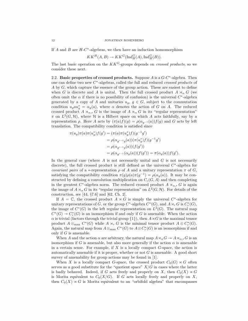
2.2. Basic properties of crossed products. Suppose A is aG-C∗-algebra. Thenone can define two new C∗-algebras, called the full and reduced crossed products ofA by G, which capture the essence of the group action. These are easiest to definewhen G is discrete and A is unital. Then the full crossed product A ⋊α G (weoften omit the α if there is no possibility of confusion) is the universal C∗-algebragenerated by a copy of A and unitaries ug, g ∈ G, subject to the commutationcondition ugau

∗g = αg(a), where α denotes the action of G on A. The reduced

crossed product A ⋊α,r G is the image of A ⋊α G in its “regular representation”π on L2(G,H), where H is a Hilbert space on which A acts faithfully, say by arepresentation ρ. Here A acts by (π(a)f)(g) = ρ(αg−1(a))f(g) and G acts by lefttranslation. The compatibility condition is satisfied since

π(ug)π(a)π(u∗g)f(g′) = (π(a)π(u∗g)f)(g−1g′)

= ρ(αg′−1g(a))(π(u∗g)f)(g−1g′)

= ρ(αg′−1g(a))(f(g′))

= ρ(αg′−1(αg(a))(f(g′)) = π(αg(a))f(g′).

In the general case (where A is not necessarily unital and G is not necessarilydiscrete), the full crossed product is still defined as the universal C∗-algebra forcovariant pairs of a ∗-representation ρ of A and a unitary representation π of G,satisfying the compatibility condition π(g)ρ(a)π(g−1) = ρ(αg(a)). It may be con-structed by defining a convolution multiplication on Cc(G,A) and then completingin the greatest C∗-algebra norm. The reduced crossed product A ⋊α,r G is againthe image of A⋊αG in its “regular representation” on L2(G,H). For details of theconstruction, see [44, §7.6] and [62, Ch. 2].

If A = C, the crossed product A ⋊ G is simply the universal C∗-algebra forunitary representations of G, or the group C∗-algebra C∗(G), and A⋊rG is C∗

r (G),the image of C∗(G) in the left regular representation on L2(G). The natural mapC∗(G)։ C∗

r (G) is an isomorphism if and only if G is amenable. When the actionα is trivial (factors through the trivial group {1}), then A⋊G is the maximal tensorproduct A ⊗max C

∗(G) while A ⋊r G is the minimal tensor product A ⊗ C∗r (G).

Again, the natural map from A⊗max C∗(G) to A⊗C∗

r (G) is an isomorphism if andonly if G is amenable.

When A and the action α are arbitrary, the natural map A⋊αG։ A⋊α,rG is anisomorphism if G is amenable, but also more generally if the action α is amenablein a certain sense. For example, if X is a locally compact G-space, the action isautomatically amenable if it is proper, whether or not G is amenable. A good shortsurvey of amenability for group actions may be found in [1].

When X is a locally compact G-space, the crossed product C0(G) ⋊ G oftenserves as a good substitute for the “quotient space” X/G in cases where the latteris badly behaved. Indeed, if G acts freely and properly on X , then C0(X) ⋊ Gis Morita equivalent to C0(X/G). If G acts locally freely and properly on X ,then C0(X) ⋊ G is Morita equivalent to an “orbifold algebra” that encompasses


not only the topology of X/G but also the finite isotropy groups. But if the G-action is not proper, X/G may be highly non-Hausdorff, while C0(X) ⋊ G maybe a perfectly well-behaved noncommutative algebra. A key case later on will theone where X = T is the circle group, G = Z, and the generator of G acts bymultiplication by e2πiθ. When θ is irrational, every orbit is dense, so X/G is anindiscrete space, and C(T) ⋊ Z is what’s usually denoted Aθ, an irrational rotation

algebra or noncommutative 2-torus.Now we can explain the relationships between equivariantKK-theory and crossed

products. One connection is that if G is discrete and A is a G-C∗-algebra, there is anatural isomorphism KKG(A,C) ∼= KK(A⋊G,C). Dually, if G is compact, thereis a natural Green-Julg isomorphism [6, §11.7] KKG(C, A) ∼= KK(C, A⋊G). Stillanother connection is that there is (for arbitrary G) a functorial homomorphism

j : KKG(A,B) → KK(A⋊G,B ⋊G)

sending (when B = A) 1A to 1A⋊G. (In fact, j can be viewed as a functor from

the equivariant Kasparov category KKG to the non-equivariant Kasparov categoryKK. Later we will study how close it is to being faithful.) There is also a variant ofj using reduced crossed products, denoted jr [35, §3.11]. If B = C and G is discrete,then j can be identified with the map KK(A⋊G,C) → KK(A⋊G,C∗(G)) inducedby the inclusion of scalars C → C∗(G). (The fact that G is discrete means thatC∗(G) is unital.) The map j is split injective in this case since it is split by the mapinduced by C∗(G) → C, corresponding to the trivial representation of G. Similarly,if G is compact, then via Green-Julg, j can be identified with the map KK(C, A⋊

G) → KK(C∗(G), A ⋊ G) induced by the map C∗(G) → C corresponding to thetrivial representation of G. This is again a split injection since C∗(G) splits as thedirect sum of C and summands associated to other representations.

2.3. The dual action and Takai duality. When the group G is not just locally

compact but also abelian, then it has a Pontrjagin dual group G. In this case, givenany G-C∗-algebra algebra A, say with α denoting the action of G on A, there is

a dual action α of G on the crossed product A ⋊ G. When A is unital and G isdiscrete, so that A ⋊ G is generated by a copy of A and unitaries ug, g ∈ G, thedual action is given simply by

αγ(aug) = aug〈g, γ〉.

The same formula still applies in general, except that the elements a and ug don’tquite live in the crossed product but in a larger algebra. The key fact about the

dual action is the Takai duality theorem: (A⋊αG) ⋊bα G ∼= A⊗K(L2(G)), and the

double dual action ˆα of ˜G ∼= G on this algebra can be identified with α ⊗ Adλ,where λ is the left regular representation of G on L2(G). Good expositions may befound in [44, §7.9] and in [62, Ch. 7].

2.4. Connes’ “Thom isomorphism”. Recall that the Thom isomorphism the-orem in K-theory (see Section 1.1) asserts that if E is a complex vector bundleover X , there is an isomorphism of K-groups K(X) → K(E), implemented bya KK-class in KK(X,E). Now if Cn (or R2n — there is no difference sincewe are just considering the additive group structure) acts on X by a trivial ac-

tion α, then C0(X) ⋊α Cn ∼= C0(X) ⊗ C∗(Cn) ∼= C0(X) ⊗ C0(Cn) ∼= C0(E),


where E is a trivial rank-n complex vector bundle over X . (We have used Pon-trjagin duality and the fact that abelian groups are amenable.) It follows thatK(C0(X)) ∼= K(C0(X) ⋊α Cn). Since any action α of Cn is homotopic to thetrivial action and “K-theory is supposed to be homotopy invariant,” that suggeststhat perhaps KK(A) ∼= KK(A⋊α Cn) for any C∗-algebra A and for any action αof Cn. This is indeed true and the isomorphism is implemented by classes (whichare inverse to one another) in KK(A,A⋊α Cn) and KK(A⋊α Cn, A). It is clearlyenough to prove this in the case n = 1, since we can always break a crossed productby Cn up as an n-fold iterated crossed product.

That A and A ⋊α C are always KK-equivalent or that they at least have thesame K-theory, or (this is equivalent since one can always suspend on both sides)that A ⊗ C0(R) and A ⋊α R are always KK-equivalent or that they at least havethe same K-theory for any action of R, is called Connes’ “Thom isomorphism”

(with the name “Thom” in quotes since the only connection with the classicalThom isomorphism is the one we have already explained). Connes’ original proofis relatively elementary, but only gives an isomorphism of K-groups, not a KK-equivalence, and can be found in [12] or in [20, §10.2].

To illustrate Connes’ idea, let’s suppose A is unital and we have a class inK0(A) represented by a projection p ∈ A. (One can always reduce to this specialcase.) If α were to fix p, then 1 7→ p gives an equivariant map from C to A

and thus would induce a map of crossed products C ⋊ R ∼= C0(R) → A ⋊α R or

C ⋊ C ∼= C0(C) → A ⋊α C giving a map on K-theory β : Z → K0(A ⋊ C). Theimage of [p] under the isomorphism K0(A) → K0(A⋊C) will be β(1). So the idea isto show that one can modify the action to one fixing p (using a cocycle conjugacy)without changing the isomorphism class of the crossed product.

There are now quite a number of proofs of Connes’ theorem available, each usingsomewhat different techniques. We just mention a few of them. A proof using K-theory of Wiener-Hopf extensions is given in [49]. There are also fancier proofs usingKK-theory. If α is a given action of R on A and if β is the trivial action, one can tryto construct KKR elements c ∈ KKR((A,α), (A, β)) and d ∈ KKR((A, β), (A,α))

which are inverses of each other in KKR. Then the morphism j of Section 2.1 sendsthese to KK-equivalences j(c) and j(d) between A⋊α R and A⋊β R ∼= A⊗C0(R).

Another rather elegant approach, using KK-theory but not the equivariantgroups, may be found in [26]. Fack and Skandalis use the group KK1(A,B), whichwe have avoided so far in order to simplify the theory, but it can be defined withtriples (H, φ, T ) like those used for KK(A,B), but with two modifications:

(1) H is no longer graded, and there is no grading condition on φ.(2) T is self-adjoint but with no grading condition, and φ(a)(T 2 − 1) ∈ K(H)

and [φ(a), T ] ∈ K(H) for all a ∈ A.

It turns out that KK1(A,B) ∼= KK(A⊗C0(R), B), and that the Kasparov productcan be extended to a graded commutative product on the direct sum ofKK = KK0

and KK1. The product of two classes in KK1 can by Bott periodicity be taken toland in KK0.

We can now explain the proof of Fack and Skandalis as follows. They show thatfor each separable C∗-algebra A with an action α of R, there is a special elementtα ∈ KK1(A,A⋊αR) (constructed using a singular integral operator). Note by theway that doing the construction with the dual action and applying Takai duality


gives tbα ∈ KK1(A⋊αR, A), since (A⋊αR)⋊bαR ∼= A⊗K, which is Morita equivalentto A. These elements have the following properties:

(1) (Normalization) If A = C (so that necessarily α = 1 is trivial), then t1 ∈KK1(C, C0(R)) is the usual generator of this group (which is isomorphicto Z).

(2) (Naturality) The elements are natural with respect to equivariant homo-morphisms ρ : (A,α) → (C, γ), in that if ρ denotes the induced map oncrossed products, then ρ∗(tα) = ρ∗(tγ) ∈ KK(A,C ⋊γ R), and similarly,ρ∗(tbγ) = ρ∗(tbα) ∈ KK(A⋊α R, C).

(3) (Compatibility with external products) Given x ∈ KK(A,B) and y ∈KK(C,D),

(tbα ⊗A x)⊠ y = tα⊗1C

⊗A⊗C (x⊠ y).

Similarly, given x ∈ KK(B,A) and y ∈ KK(D,C),

y ⊠ (x⊗A tα) = (y ⊠ x) ⊗C⊗A t1C⊗α. �

Theorem 2.1 (Fack-Skandalis [26]). These properties completely determine tα,and tα is a KK-equivalence (of degree 1) between A and A⋊α R.

Proof. Suppose we have elements tα satisfying the properties above. Let us firstshow that tα⊗A⋊αRtbα = 1A. For s ∈ R, let αs be the rescaled action αst = αst. Thendefine an action β of R on B = C([0, 1], A) by (βtf)(s) = αst (f(s)). Let gs : B → Abe evaluation at s, which is clearly an equivariant map (B, β) ։ (A,αs). We also

get maps gs : B⋊βR → A⋊αs R, and the double dual map ˆgs can be identified withgs⊗1: B⊗K → A⊗K. By Axiom (2), (gs)∗(tβ) = g∗s(tαs) and (gs)∗(tbβ) = g∗s(tbαs).

Let σs = tαs ⊗A⋊αsR tbαs ∈ KK(A,A). By associativity of Kasparov products,

(gs)∗(tβ ⊗B⋊βR tbβ

)= tβ ⊗B⋊βR

(tbβ ⊗B [gs]

)

= tβ ⊗B⋊βR

([gs] ⊗A⋊αsR tbαs

)

=(tβ ⊗B⋊βR [gs]

)⊗A⋊αsR tbαs

=([gs] ⊗A tαs

)⊗A⋊αs R tbαs

= [gs] ⊗A σs.

Since gs is a homotopy of maps B → A and KK is homotopy-invariant, [gs] = [g0].But g0 is a homotopy equivalence with homotopy inverse f : a 7→ a⊗ 1, so we seethat

σs = [f ] ⊗B(tβ ⊗B⋊βR tbβ

)⊗B [g0]

is independent of s. In particular, σ1 = tα ⊗A⋊αR tbα agrees with σ0, which can becomputed to be 1A by Axioms (1) and (3) since the action of R is trivial in thiscase. So tα ⊗A⋊αR tbα = 1A. Replacing α by α and using Takai duality, this alsoimplies that tbα ⊗A tα = 1A⋊αR. So tα and tbα give KK-equivalences.

The uniqueness falls out at the same time, since we see from the above that[gs] ⊗A tαs = tβ ⊗B⋊βR [gs] ∈ KK(B,A ⋊αs R), and that all the KK-elementsinvolved are KK-equivalences. Furthermore, we know by Axioms (1) and (3) thattα0 = 1A ⊠ t1, where t1 is the special element of KK1(C, C0(R)) mentioned inAxiom (1). This determines tβ (from the identity [g0]⊗A tα0 = tβ ⊗B⋊βR [g0]), andthen tα is determined from the identity [g0] ⊗A tα = tβ ⊗B⋊βR [g1]. �


2.5. The Pimsner-Voiculescu Theorem. Connes’ Theorem from Section 2.4computes K-theory or KK-theory for crossed products by R. This can be used tocompute K-theory or KK-theory for crossed products by Z, using the fact fromSection 2.2 that if A is a C∗-algebra equipped with an action α of Z (or equivalently,a single ∗-automorphism θ, the image of 1 ∈ Z under the action), then A ⋊α Z is

Morita equivalent to(IndR

Z(A,α))

⋊R. The algebra Tθ = IndR

Z(A,α) is often called

the mapping torus of (A, θ); it can be identified with the algebra of continuousfunctions f : [0, 1] → A with f(1) = θ(f(0)). It comes with an obvious short exactsequence

0 → C0((0, 1), A) → Tθ → A→ 0,

for which the associated exact sequence in K-theory has the form

· · · → K1(A)1−θ∗−−−→ K1(A) → K0(Tθ) → K0(A)

1−θ∗−−−→ K0(A) → · · · .

Since

K0(A⋊α Z) ∼= K0(Tθ ⋊Indα R) ∼= K1(Tθ),

and similarly for K0, we obtain the Pimsner-Voiculescu exact sequence

(2.1)· · · → K1(A)

1−θ∗−−−→ K1(A) → K1(A⋊α Z) →

→ K0(A)1−θ∗−−−→ K0(A) → K0(A⋊α Z) → · · · .

Here one can check that the mapsKj(A) → Kj(A⋊αZ) are induced by the inclusionof A into the crossed product. For another proof, closer to the original argumentof Pimsner and Voiculescu, see [20, Ch. 5].

2.6. The Baum-Connes Conjecture. The theorems of Connes and Pimsner-Voiculescu on K-theory of crossed products by R and Z suggest the question ofwhether there are similar results for other groups G. In particular, one would liketo know if the K-theory of C∗

r (G), or better still, the K-theory of reduced crossedproducts A ⋊ G, can be computed in a “topological” way. The answer in manycases seems to be “yes,” and the conjectured answer is what is usually called theBaum-Connes Conjecture, with or without coefficients. The special case of theBaum-Connes Conjecture (without coefficients) for connected Lie groups is alsoknown as the Connes-Kasparov Conjecture, and is now a known theorem.

The Baum-Connes conjecture also has other origins, such as the Novikov Con-jecture on higher signatures and conjectures about algebraic K-theory of grouprings, which will be touched on in Reich’s lectures. These other motivations for theconjecture mostly concern the case where G is discrete, which is actually the mostinteresting case of the conjecture, though there are good reasons for not restrictingonly to this case. (For example, as we already saw in the case of Z, informationabout discrete groups can often be obtained by embedding them in a Lie group.)

Here is the formal statement of the conjecture.

Conjecture 2.2 (Baum-Connes). Let G be a locally compact group, second-coun-

table for convenience. Let EG be the universal proper G-space. (This is a con-

tractible space on which G acts properly, characterized [5] up to G-homotopy equiv-

alence by two properties: that every compact subgroup of G has a fixed point in EG,

and that the two projections EG × EG → EG are G-homotopic. Here the product


space is given the diagonal G-action. If G has no compact subgroups, then EG is

the usual universal free G-space EG.) There is an assembly map

lim−→

X⊆EGX/G compact

KG∗ (X) → K∗(C

∗r (G))

defined by taking G-indices of G-invariant elliptic operators, and this map is an

isomorphism.

Conjecture 2.3 (Baum-Connes with coefficients). With notation as in Conjecture

2.2, if A is any separable G-C∗-algebra, the assembly map

lim−→

X⊆EGX/G compact

KKG∗ (C0(X), A) → K∗(A⋊r G)

is an isomorphism.

Let’s see what the conjecture amounts to in some special cases. If G is compact,EG can be taken to be a single point. The conjecture then asserts that the assembly

map KKG∗ (pt, pt) → K∗(C

∗(G)) is an isomorphism. For G compact, C∗(G) is bythe Peter-Weyl Theorem the completed direct sum of matrix algebras

⊕V End(V ),

where V runs over a set of representatives for the irreducible representations ofG. Thus K1(C

∗(G)) (remember this is topological K1) vanishes and K0(C∗(G)) ∼=

R(G). The assembly map in this case is the Green-Julg isomorphism of Section2.2. In fact, the same holds with coefficients; the assembly map KKG

∗ (C, A) =KG

∗ (A) → K∗(A⋊G) is the Green-Julg isomorphism, and Conjecture 2.3 is true.Next, suppose G = R. Since G has no compact subgroups and is contractible, we

can take EG = R with R acting on itself by translations. If A is an R-C∗-algebra,the assembly map is a map KKR

∗ (C0(R), A) → K∗(A⋊ R). This map turns out tobe Kasparov’s morphism

j : KKR∗ (C0(R), A) → KK∗(C0(R) ⋊ R, A⋊ R) = KK∗(K, A⋊ R) ∼= K∗(A⋊ R),

which is the isomorphism of Connes’ Theorem (Section 2.4). (The isomorphismC0(R) ⋊ R ∼= K is a special case of the Imprimitivity Theorem giving a Morita

equivalence between(IndG{1}A

)⋊G and A, or if you prefer, of Takai duality from

Section 2.3.) So again the conjecture is true.Another good test case is G = Z. Then EG = EG = R, with Z acting by

translations and quotient space T. The left-hand side of the conjecture is thusKKZ(C0(R), A), while the right-hand side is K(A⋊ Z), which is computed by thePimsner-Voiculescu sequence.

More generally, suppose G is discrete and torsion-free. Then EG = EG, andthe quotient space EG/G is the usual classifying space BG. The assembly map

(for the conjecture without coefficients) maps Kcmpct∗ (BG) → K∗(C

∗r (G)). (The

left-hand side is K-homology with compact supports.) This map can be viewed asan index map, since classes in the K-homology group on the left are representedby generalized Dirac operators D over Spinc manifolds M with a G-covering, andthe assembly map takes such an operator to its “Mishchenko-Fomenko index” withvalues in the K-theory of the (reduced) group C∗-algebra. The connection betweenthis assembly map and the usual sort of assembly map studied by topologists isdiscussed in [55]. In particular, Conjecture 2.2 implies a strong form of the NovikovConjecture for G.


2.7. The approach of Meyer and Nest. An interesting alternative approachto the Baum-Connes Conjecture has been proposed by Meyer and Nest [42, 43].This approach is also briefly sketched (in somewhat simplified form) in [20, §5.3]and in [56, Ch. 5]. Meyer and Nest begin by observing that the equivariant KK-

category, KKG, naturally has the structure of a triangulated category. It has adistinguished class E of weak equivalences, morphisms f ∈ KKG(A,B) which re-strict to equivalences in KKH(A,B) for every compact subgroup H of G. (Notethat if G has no nontrivial compact subgroups, for example if G is discrete andtorsion-free, then this condition just says that f is a KK-equivalence after forget-ting the G-equivariant structure.) The Baum-Connes Conjecture with coefficients,Conjecture 2.3, basically amounts to the assertion that if f ∈ KKG(A,B) is in E ,then jr(f) ∈ KK(A ⋊r G,B ⋊r G) is a KK-equivalence.2 In particular, supposeG has no nontrivial compact subgroups and satisfies Conjecture 2.3. Then if Ais a G-C∗-algebra which, forgetting the G-action, is contractible, then the uniquemorphism in KKG(0, A) is a weak equivalence, and so (applying jr), the uniquemorphism in KK(0, A⋊r G) is a KK-equivalence. Thus A⋊r G is K-contractible,i.e., all of its topological K-groups must vanish. When G = R, this follows fromConnes’ Theorem, and when G = Z, this follows from the Pimsner-Voiculescu exactsequence, (2.1).

Now that we have several different formulations of the Baum-Connes Conjecture,it is natural to ask how widely the conjecture is valid. Here are some of the thingsthat are known:

(1) There is no known counterexample to Conjecture 2.2 (Baum-Connes forgroups, without coefficients). Counterexamples are now known [27] to Con-jecture 2.3 with G discrete and A even commutative.

(2) Conjecture 2.3 is true if G is amenable, or more generally, if it is a-T-

menable, that is, if it has an affine, isometric and metrically proper action ona Hilbert space [30]. Such groups include all Lie groups whose noncompactsemisimple factors are all locally isomorphic to SO(n, 1) or SU(n, 1) forsome n.

(3) Conjecture 2.2 is true for connected reductive Lie groups, connected reduc-tive p-adic groups, for hyperbolic discrete groups, and for cocompact latticesubgroups of Sp(n, 1) or SL(3,C) [39].

There is now a vast literature on this subject, but our intention here is not tobe exhaustive, but just to give the reader some flavor of what’s going on.

2The reason for using jr in place of j for can be seen from the case of G nonamenable with

property T. In this case, C∗(G) has a projection corresponding to the trivial representation of G

which is “isolated,” and thus maps to 0 in C∗

r(G). So these two algebras do not have the same

K-theory. It turns out at least in many examples that K0(C∗

r(G)) can be described in purely

topological terms, but K0(C∗(G)) cannot.


Lecture 3. The universal coefficient theorem for KK and some of

its applications

3.1. Introduction to the UCT. Now that we have discussed KK and KKG,a natural question arises: how computable are they? In particular, is KK(A,B)determined by K∗(A) and by K∗(B)? Is KKG(A,B) determined by KG

∗ (A) andby KG

∗ (B)?A first step was taken by Kasparov [34]: he pointed out that KK(X,Y ) is given

by an explicit topological formula when the one-point compactifications X+ and

Y+ are finite CW complexes: KK(X,Y ) ∼= K(Y+∧D(X+)), where D(X+) denotesthe Spanier-Whitehead dual of X+.3

Let’s make a definition — we say the pair of C∗-algebras (A,B) satisfies the

Universal Coefficient Theorem for KK (or UCT for short) if there is an exactsequence

(3.1) 0 →⊕

∗∈Z/2

Ext1Z(K∗(A),K∗+1(B)) → KK(A,B)

ϕ−→

⊕

∗∈Z/2

HomZ(K∗(A),K∗(B)) → 0.

Here ϕ sends a KK-class to the induced map on K-groups.We need one more definition. Let B be the bootstrap category, the smallest

full subcategory of the separable C∗-algebras (with the ∗-homomorphisms as mor-phisms) containing all separable type I algebras, and closed under extensions,countable C∗-inductive limits, and KK-equivalences. Note that KK-equivalencesinclude Morita equivalences, and type I algebras include commutative algebras.Recall from Section 1.2 that stably isomorphic separable C∗-algebras are Moritaequivalent, hence KK-equivalent. Furthermore, separable type I C∗-algebras areinductive limits of finite iterated extensions of stably commutative C∗-algebras [44,Ch. 6]. Thus we could just as well replace the words “type I” by “commutative” inthe definition of B. Furthermore, any compact metric space is a countable limit offinite CW complexes. Dualizing, that means that any unital separable commutativeC∗-algebra is a countable inductive limit (i.e., categorical colimit) of algebras of theform C(X), X a finite CW complex, and any separable commutative C∗-algebrais a countable inductive limit (i.e., colimit) of algebras of the form C0(X), X+ afinite CW complex. We will use this fact shortly.

Theorem 3.1 (Rosenberg-Schochet [58]). The UCT holds for all pairs (A,B) with

A an object in B and B separable.

Unsolved problem: Is every separable nuclear C∗-algebra in B? Skandalis [60]showed that there are non-nuclear algebras not in B, for which the UCT fails.

3.2. The proof of Rosenberg and Schochet. First suppose K∗(B) is injectiveas a Z-module, i.e., divisible as an abelian group. Then HomZ( ,K∗(B)) is anexact functor, so A 7→ HomZ(K∗(A),K∗(B)) gives a cohomology theory on C∗-algebras. In particular, ϕ is a natural transformation of homology theories forspaces (

X 7→ KK∗(C0(X), B))

(X 7→ HomZ(K∗(X),K∗(B))

).

3Spanier-Whitehead duality basically interchanged homology and cohomology. ∧ denotes thesmash product, the product in the category of spaces with distinguished basepoint.


Since ϕ is an isomorphism for X = Rn by Bott periodicity, it is an isomorphismwhenever X+ is a sphere, and thus (by the analogue of the Eilenberg-Steenroduniqueness theorem for generalized homology theories) whenever X+ is a finiteCW complex.

We extend to arbitrary locally compact X by taking limits, and then to the restof B, using the observations we made before the proof of the theorem. In order toknow we can pass to countable inductive limits, we need one additional fact aboutKK, namely that it is “countably additive” (sends countable C∗-algebra directsums in the first variable to products of abelian groups). This fact is not hard tocheck from Kasparov’s original definition. So the theorem holds when K∗(B) isinjective.

The rest of the proof uses an idea due to Atiyah [3], of geometric resolutions.The idea is that given arbitrary B, we can change it up to KK-equivalence so thatit fits into a short exact sequence

0 → C → B → D → 0

for which the induced K-theory sequence is short exact:

K∗(B) K∗(D)։ K∗−1(C)

and K∗(D), K∗(C) are Z-injective. Then we use the theorem for KK∗(A,D) andKK∗(A,C), along with the long exact sequence in KK in the second variable, toget the UCT for (A,B). �

3.3. The equivariant case. If one asks about the UCT in the equivariant case,then the homological algebra of the ground ring R(G) becomes relevant. This isnot always well behaved, so as noticed by Hodgkin [31], one needs restrictions on Gto get anywhere. But for G a connected compact Lie group with π1(G) torsion-free,R(G) has finite global dimension, and the spectral sequence one ends up with doesconverge to the right limit.

Theorem 3.2 (Rosenberg-Schochet [57]). If G is a connected compact Lie group

with π1(G) torsion-free, and if A, B are separable G-C∗-algebras with A in a suit-

able bootstrap category containing all commutative G-C∗-algebras, then there is a

convergent spectral sequence

ExtpR(G)(KG∗ (A),KG

q+∗(A)) ⇒ KKG∗ (A,B).

The proof is more complicated than in the non-equivariant case, but in the samespirit.

Also along the same lines, there is a UCT for KK of real C∗-algebras, due toBoersema [8]. The homological algebra involved in this case is appreciably morecomplicated than in the complex C∗-algebra case, and is based on ideas on Bousfield[9] on the classification of K-local spectra.

3.4. The categorical approach. The UCT implies a lot of interesting facts aboutthe bootstrap category B. Here are a few examples.

Theorem 3.3 (Rosenberg-Schochet [58]). Let A, B be C∗-algebras in B. Then

A and B are KK-equivalent if and only if they have the isomorphic topological

K-groups.


Proof. ⇒ is trivial. So suppose K∗(A) ∼= K∗(B). Choose an isomorphism

ψ : K∗(A) → K∗(B).

Since the map ϕ in the UCT (3.1) is surjective, ψ is realized by a class x ∈KK(A,B) (not necessarily unique, but just pick one).

Now consider the commutative diagram with exact rows

0 // Ext1Z(K∗+1(B),K∗(A)) //

ψ∗∼=

��

KK∗(B,A)ϕ

//

x⊗B

��

Hom(K∗(B),K∗(A)) //

ψ∗∼=

��

0

0 // Ext1Z(K∗+1(A),K∗(A)) // KK∗(A,A)

ϕ// Hom(K∗(A),K∗(A)) // 0

By the 5-Lemma, Kasparov product with x is an isomorphism KK∗(B,A) →KK∗(A,A). In particular, there exists y ∈ KK(B,A) with x⊗B y = 1A. Similarly,there exists z ∈ KK(B,A) with z ⊗A x = 1B. Then by associativity

z = z ⊗A (x⊗B y) = (z ⊗A x) ⊗B y = y

and we have a KK-inverse to x. �

Corollary 3.4. We can also describe B as the smallest full subcategory of the

separable C∗-algebras closed under KK-equivalence and containing the separable

commutative C∗-algebras. A separable C∗-algebra A has the property that (A,B)satisfies the UCT for all separable C∗-algebras if and only if it lies in B.

Proof. Let B′ be the smallest full subcategory of the separable C∗-algebras closedunder KK-equivalence and containing the separable commutative C∗-algebras. Bydefinition of B, B′ is a subcategory of B. But if A is in B, itsK-groups are countable.For any countable groups G0 and G1, it is easy to construct a second-countablelocally compact space with these K-groups. So there is a separable commutativeC∗-algebra C0(Y ) with K∗(C0(Y )) ∼= K∗(A) (just as abelian groups). By Theorem3.3, there is a KK-equivalence between A and C0(Y ), so A lies in B′.

As far as the last statement is concerned, one direction is the UCT itself. For theother direction, suppose that (A,B) satisfies the UCT for all separable C∗-algebrasB. In particular, it holds for a commutative B with the same K-groups as A, andby the argument above, A is KK-equivalent to B, hence lies in B. �

Recall that KK(A,A) = EndKK(A) is a ring under Kasparov product. We cannow compute the ring structure.

Theorem 3.5 (Rosenberg-Schochet). Suppose A is in B. In the UCT sequence

0 →⊕

i∈Z/2

Ext1Z(Ki+1(A),Ki(A)) → KK(A,A)ϕ−→

⊕

i∈Z/2

End(Ki(A)) → 0,

ϕ is a split surjective homomorphism of rings, and J = kerϕ (the Ext term) is an

ideal with J2 = 0.

Proof. Choose A0 and A1 commutative with K0(A0) ∼= K0(A), K1(A0) = 0,K0(A1) = 0, K1(A1) ∼= K1(A). Then by Theorem 3.3, A0⊕A1 is KK-equivalent toA, and without loss of generality, we may assume we have an actual splitting A =A0 ⊕A1. By the UCT, KK(A0, A0) ∼= EndK0(A) and KK(A1, A1) ∼= EndK1(A).

So KK(A0, A0)⊕KK(A1, A1) is a subring of KK(A,A) mapping isomorphicallyunder ϕ. This shows ϕ is split surjective. We also have J = KK(A0, A1) ⊕


KK(A1, A0). If, say, x lies in the first summand and y in the second, then x⊗A1y

induces the 0-map on K0(A) and so is 0 in KK(A0, A0) ∼= End(K0(A)). Similarly,y⊗A0

x induces the 0-map on K1(A) and so is 0 in KK(A1, A1) ∼= End(K1(A)). �

3.5. The homotopy-theoretic approach. There is a homotopy-theoretic ap-proach to the UCT that topologists might find attractive; it seems to have beendiscovered independently by several people (e.g., [11, 32] — see also the review of[11] in MathSciNet). Let A and B be C∗-algebras and let K(A) and K(B) be theirtopological K-theory spectra. These are module spectra over K = K(C), the usualspectrum of complex K-theory. Then we can define

KKtop(A,B) = π0(HomK

(K(A),K(B))

).

This is again using ideas of Bousfield [9].

Theorem 3.6. There is a natural map KK(A,B) → KKtop(A,B), and it’s an

isomorphism if and only if the UCT holds for the pair (A,B).

Observe that KKtop(A,B) even makes sense for Banach algebras, and alwayscomes with a UCT.

We promised in the first lecture to show that defining KK(X,Y ) to be the setof natural transformations

(Z 7→ K(X × Z)) (Z 7→ K(Y × Z))

indeed agrees with Kasparov’s KK(C0(X), C0(Y )). Indeed, Z 7→ K(X × Z) is ba-sically the cohomology theory defined by K(X), and Z 7→ K(Y ×Z) is similarly thecohomology theory defined by K(Y ). So the natural transformations (commutingwith Bott periodicity) are basically a model for KKtop(C0(X), C0(Y )).

3.6. Topological applications. The UCT can be used to prove facts about topo-logical K-theory which on their face have nothing to do with C∗-algebras or KK.For example, we have the following purely topological fact:

Theorem 3.7. Let X and Y be locally compact spaces such that K∗(X) ∼= K∗(Y )just as abelian groups. Then the associated K-theory spectra K(X) and K(Y ) are

homotopy equivalent.

Proof. We have seen (Theorem 3.3) that the hypothesis implies C0(X) and C0(Y )are KK-equivalent, which gives the desired conclusion. �

Note that this theorem is quite special to complex K-theory; it fails even forordinary cohomology (since one needs to consider the action of the Steenrod alge-bra).

Similarly, the UCT implies facts about cohomology operations in complex K-theory and K-theory mod p. For example, one has:

Theorem 3.8 (Rosenberg-Schochet [58]). The Z/2-graded ring of homology opera-

tions for K( ; Z/n) on the category of separable C∗-algebras is the exterior algebra

over Z/n on a single generator, the Bockstein β.

Theorem 3.9 (Araki-Toda [2], new proof by Rosenberg-Schochet in [58]). There

are exactly n admissible multiplications on K-theory mod n. When n is odd, exactly

one is commutative. When n = 2, neither is commutative.


3.7. Applications to C∗-algebras. Probably the most interesting applications ofthe UCT for KK are to the classification problem for nuclear C∗-algebras. TheElliott program (to quote M. Rørdam from his review of the Kirchberg-Phillipspaper [37]) is to classify “all separable, nuclear C∗-algebras in terms of an invariantthat has K-theory as an important ingredient.” Kirchberg and Phillips have shownhow to do this for Kirchberg algebras, that is simple, purely infinite, separable andnuclear C∗-algebras. The UCT for KK is a key ingredient.

Theorem 3.10 (Kirchberg-Phillips [37, 45]). Two stable Kirchberg algebras A and

B are isomorphic if and only if they are KK-equivalent; and moreover every in-

vertible element in KK(A,B) lifts to an isomorphism A → B. Similarly in the

unital case if one keeps track of [1A] ∈ K0(A).

We will not attempt to explain the proof of Kirchberg-Phillips, but it’s basedon the idea that a KK-class is given by a quasihomomorphism, which under thespecific hypotheses can be lifted to a true homomorphism. More recent results ofa somewhat similar nature may be found in [22, 21, 41].

Given the Kirchberg-Phillips result, one is still left with the question of deter-mining when two Kirchberg algebras are KK-equivalent. But those of “Cuntztype” (like On)

4 lie in B, and Kirchberg and Phillips show that ∀ abelian groupsG0 and G1 and ∀g ∈ G0, there is a nonunital Kirchberg algebra A ∈ B with theseK-groups, and there is a unital Kirchberg algebra A ∈ B with these K-groups andwith [1A] = g. By the UCT, these algebras are classified by their K-groups.

The original work on the Elliott program dealt with the opposite extreme: stablyfinite algebras. Here again, KK can play a useful role. Here is a typical result fromthe vast literature:

Theorem 3.11 (Elliott [23]). If A and B are C∗-algebras of real rank 0 which

are inductive limits of certain “basic building blocks”, then any x ∈ KK(A,B)preserving the “graded dimension range” can be lifted to a ∗-homomorphism. If xis a KK-equivalence, it can be lifted to an isomorphism.

This theorem applies for example to the irrational rotation algebras Aθ, becauseof an amazing result by Elliott and Evans [24] that shows that these algebras areindeed inductive limits of the required type.

4This is the fundamental example of a Kirchberg algebra, invented by Cuntz [16]. It is the

universal C∗-algebra generated by n isometries whose range projections are orthogonal and add to1. Cuntz proved that it is simple, and showed that On ⊗K is a crossed product of a UHF algebra(an inductive limit of matrix algebras) by an action of Z. But crossed products by Z preserve thecategory B, because of the arguments in Sections 2.4 and 2.5. Thus On lies in B.


Lecture 4. A fundamental example in noncommutative geometry:

topology and geometry of the irrational rotation

algebra

4.1. Basic facts about Aθ. We previously mentioned the algebra Aθ, defined tobe the crossed product C(T) ⋊αθ

Z, where T is the circle group (thought of asthe unit circle in C) and where αθ sends the generator 1 ∈ Z to multiplicationby e2πiθ, i.e., rotation of the circle by an angle of 2πθ. This makes sense for anyθ ∈ R, but of course only the class of θ mod Z matters, so we might as welltake θ ∈ [0, 1). This algebra has two standard names: a rotation algebra (withparameter θ), or irrational rotation algebra in the most important case of θ /∈ Q,or a noncommutative (2-)torus, because of the fact that when θ = 0, we get backsimply C(T2), the continuous functions on the usual 2-torus. It is no exaggerationto say that these C∗-algebras are the most important examples in (C∗-algebraic)noncommutative geometry.

In this section we’ll try to lay out the basic facts about these algebras, withoutattempting to prove everything or to explain the history of every result. Thestandard references for a lot of this material are the fundamental papers of Rieffel[48, 51]. A more extensive survey on this material can be found in [53].

We can describe the algebra Aθ quite concretely, using the definition of thecrossed product in Section 2.2. The algebra has two unitary generators U andV , one of them generating C(T) and the other corresponding to the generator ofZ. They satisfy the commutation relation UV = e2πiθV U . The algebra Aθ is thecompletion of the noncommutative polynomials in U and V . But because of thecommutation relation, we can move all U ’s to the left and all V ’s to the right inany noncommutative monomial in U and V , at the expense of a scalar factor ofmodulus 1. Thus Aθ is the completion of the polynomials

∑m,n cm,nU

mV n (with

only finitely many non-zero coefficients). In fact, every element of Aθ is representedby a formal such infinite sum, but it is not so easy to describe the C∗-algebra normin terms of the sequence of Fourier coefficients {cm,n}. The one thing we can say,since ‖U‖ = ‖V ‖ = 1, is that the C∗-norm is bounded by the L1-norm, so that if thecoefficients converge absolutely, then the corresponding infinite sum does representan element of Aθ. (But the converse is false. This is classical when θ = 0, andamounts to the fact that there are continuous functions whose Fourier series do notconverge absolutely.)

The algebra Aθ has a canonical trace τ , i.e., a bounded linear functional withτ(ab) = τ(ba) for all a, b ∈ Aθ. We normalize by taking τ(1) = 1. Usually we addthe condition that τ should send self-adjoint elements to real values, though whenθ is irrational, this is automatic. When θ = 0, τ is just integration with respect toHaar measure on T2 (normalized to be a probability measure).

There is a basic dichotomy between two cases. If θ is irrational, then no differentpowers of e2πiθ coincide. It is not too hard to show from this that Aθ is simple andthat there is a unique trace in this case, defined by the condition that τ(UmV n) = 0if m 6= 0 or n 6= 0. (Recall we do require τ(1) = 1.) So τ simply picks out the(0, 0) coefficient c0,0 from

∑m,n cm,nU

mV n. On the other hand, if θ = pq ∈ Q,

then Aθ has a big center, and in fact Aθ is the algebra of sections of a bundle ofmatrix algebras over T 2. In fact one can show in this case that Aθ ∼= EndT 2(V ),the bundle endomorphisms of any complex line bundle V over T 2 with first Chernclass ≡ p (mod q) (times the usual generator of H2(T 2,Z)). The algebra has many


traces in this case, but it’s still convenient to let τ be the one with τ(UmV n) = 0if m 6= 0 or n 6= 0. (This along with the condition that τ(1) = 1 then determines τuniquely.)

The K-theory of Aθ can be computed from the Pimsner-Voiculescu sequence ofSection 2.5. In fact, the main motivation of Pimsner and Voiculescu for developingthis sequence was to compute K∗(Aθ). Since αθ is isotopic to the trivial action,regardless of the value of θ, the map 1 − α(1)∗ in (2.1) is always 0. Hence, justas abelian groups, one always has K0(Aθ) ∼= K1(Aθ) ∼= Z2. But one wants morethan this; one wants a description of the generators. Tracing through the variousmaps involved shows that one summand in K0 is generated by the rank-one freemodule (or the projection 1), and that the two summands in K1 are generated byU and V , respectively. But the interesting feature is the order structure on K0,which comes from the inclusions of projective modules. Note that the trace givesa homomorphism from K0(Aθ) to R, sending a projective module to the trace ofa self-adjoint projection (in some matrix algebra) representing it. (It’s a fact thatevery idempotent in a C∗-algebra is similar to a self-adjoint one; see for example[6, §4.6]. Since the trace takes real values on self-adjoint elements, the dimensionof a projection is real-valued.)

Theorem 4.1. If θ 6∈ Q, the trace τ induces an isomorphism of K0(Aθ) with Z+θZas ordered groups. If θ ∈ Q, then τ still sends K0(Aθ) to Z + θZ (which is equal to

θZ in this case), but is no longer an isomorphism.

The original proof of this theorem was nonconstructive, i.e., it did not exhibit aprojective module of dimension θ that should be the missing generator of K0. Wewill talk about this issue later in Section 4.3.

It follows from Theorem 4.1 that the irrational rotation algebras must split intouncountably many Morita equivalence classes, since it is easy to see that Moritaequivalence preserves the ordering on K0, and since there are uncountably manyorder isomorphism classes of subgroups of R of the form Z + θZ. In fact, any orderisomorphism Z + θZ → Z + θ′Z must be given by multiplication by some t 6= 0 inR, with the property that t ∈ Z + θ′Z and tθ ∈ Z + θ′Z. If we write t = cθ′ + d andtθ = aθ′ + b, a, b, c, d ∈ Z, then

θ =

(a bc d

)· θ′

for the usual action of 2 × 2 matrices by linear fractional transformations. Sincethe Morita equivalence must be invertible, we also have

(a bc d

)∈ GL(2,Z).

So Morita equivalences of irrational rotation algebras correspond to the action ofGL(2,Z) by linear fractional transformations. The converse is also true.

Theorem 4.2 (Rieffel). Any unital C∗-algebra Morita equivalent to an irrational

rotation algebra Aθ is a matrix algebra over Aθ′ with θ′ in the orbit of θ for the

action of GL(2,Z) on RP1 by linear fractional transformations. Every matrix in

GL(2,Z) gives rise to such a Morita equivalence.

This is not true by “general nonsense” but requires an explicit construction,which arises from the following theorem of Rieffel:


Theorem 4.3 (Rieffel [50]). If G is a locally compact group with closed subgroups

H and K, then H ⋉ (G/K) and (H\G) ⋊K are Morita equivalent.

If we apply this with G = R, H = 2πZ, and K = 2πθZ, then H\G is theusual model of T and (H\G) ⋊ K is Aθ, while H ⋉ (G/K) is A1/θ. The Moritaequivalence bimodule between these two algebras is a completion of S(R), withthe two generators of each algebra acting by translation and by multiplication byan exponential, respectively. The reason why the two actions commute is thattranslation by Z commutes with multiplication by e2πis, while translation by 1

θZ

commutes with multiplication by e2πiθs.The other Morita equivalences required by the theorem can be constructed sim-

ilarly.

4.2. Basic facts about A∞θ . One of the interesting things about Aθ is that it

behaves in many ways like a smooth manifold. That means that we should have ananalogue of the C∞ functions inside the algebra of “continuous” functions Aθ. Tofind this, note that Aθ carries an action of the compact Lie group T2 via (z, w) ·U =zU, (z, w) ·V = wV , for z, w ∈ T (viewed as complex numbers of modulus 1). Thisis analogous to the action of T2 on itself by translations. The smooth subalgebra

A∞θ is defined to be the set of C∞ vectors for this action, i.e., the elements a

for which (z, w) 7→ (z, w) · a is C∞ as a map T2 → Aθ. Alternatively, we candescribe A∞

θ as the intersection of the domains of all polynomials in δ1 and δ2, the(unbounded) derivations obtained by differentiating the action. Since it is obviousthat δ1(U) = 2πiU and δ2(U) = 0, while δ2(V ) = 2πiV and δ1(V ) = 0, one readilysees (as in the smooth case) that A∞

θ is a subalgebra and that it can be describedas

A∞θ =

{∑

m,n

cm,nUmV n | cm,n is rapidly decreasing

},

where “rapidly decreasing” means decreasing faster than the reciprocal of any pos-itive polynomial in m and n. Thus A∞

θ is isomorphic as a topological vector space(not as an algebra) to S(Z2) and then by Fourier transform to C∞(T2).

Proposition 4.4. The inclusion of A∞θ into Aθ is “isospectral” (i.e., an element

of the subalgebra is invertible in the subalgebra if and only if it has an inverse in

the larger algebra), and thus the inclusion A∞θ → Aθ induces an isomorphism on

K-theory.

Proof. Isospectral inclusions preserve K0 and (topological) K1, by the “Karoubidensity theorem,” so it is enough to prove the first statement. But this followsfrom the characterization of A∞

θ in terms of derivations, and the familiar identityδj(a

−1) = −a−1δj(a)a−1, iterated many times. �

From this Proposition, as well as the fact that there is no essential differencebetween smooth and purely topological manifold topology in dimension 2, one mightbe tempted to guess that Aθ and A∞

θ behave similarly in all important respects.But a deep fact is that this is false; Aut(Aθ) and Aut(A∞

θ ) are quite different fromone another.

Theorem 4.5. If θ is irrational, every automorphism of A∞θ is “orientation-

preserving,” i.e., the determinant of the induced map on K1(Aθ) ∼= Z2 is +1.On the other hand, Aθ has orientation-reversing automorphisms.


Comment: The first part of this is due to [19]. The second part is due to Elliottand Evans [24, 23].

4.3. Geometry of vector bundles. In classical topology, vector bundles play animportant role in studying compact manifolds M . Recall Swan’s Theorem ([6, §1.7]or [20, §1.3.3]): there is an equivalence of categories between topological (respec-tively, smooth) vector bundles over M and finitely generated projective modulesover C(M) (resp., C∞(M)). Thus in noncommutative geometry, finitely generatedprojective modules play the same role as vector bundles. Because of Proposition4.4, when it comes to irrational rotation algebras, the “vector bundle” theory isessentially the same in both the continuous and C∞ cases, in that every finitelygenerated projective module overAθ is extended from a finitely generated projectivemodule over A∞

θ , which is unique up to isomorphism.Now K-theory gives the stable classification of vector bundles. The unstable

classification is always more delicate, but for Aθ, this, too is known:

Theorem 4.6 (Rieffel [51]). For Aθ with θ irrational, complete cancellation holds

for finitely generated projective modules, i.e., if P ⊕Q ∼= P ′⊕Q as Aθ-modules, for

any finitely generated projective Aθ-modules P, P ′, Q, then P and P ′ are isomorphic.

The isomorphism classes of projective submodules of a free Aθ-module of rank n are

distinguished by the trace, and are given exactly by elements of K0(Aθ) ∼= Z + θZbetween 0 and n (inclusive).

Once one knows the classification of the “vector bundles,” in both the smoothand continuous categories, a natural next step is to study “geometry” on them. Inhis fundamental paper [14], Alain Connes explained how the theory of connectionsand curvature in differential geometry can be carried over to the noncommutativecase, at least when one has an algebra A like Aθ with an action of a Lie group Gfor which the “smooth subalgebra” A∞ is the set of C∞-vectors for the G-actionon A. (This of course applies here with G = T2 acting as we described above.)Then if V is a finitely generated (right) A∞-module, a connection on V is a map∇ : V → V ⊗ g

∗ (g the Lie algebra of G) satisfying the usual Leibniz rule

∇X(v · a) = ∇X(v) · a+ v · (X · a), v ∈ V, a ∈ A∞, X ∈ g.

Usually one requires a connection to be compatible with an inner product also.

Connections always exist and have a curvature 2-form Θ ∈ EndA(V )⊗∧2

g∗ defined

as usual byΘ(X,Y ) = ∇X∇Y −∇Y∇X −∇[X,Y ].

Theorem 4.7 (Connes [14]). Every finitely generated projective module over A∞θ

admits a connection of constant curvature (i.e., with the curvature in i∧2

g∗). The

curvature can be taken to be 0 if and only if the module is free. More precisely, on

the projective module with “dimension” p+ qθ > 0, p, q ∈ Z, the constant curvature

connections have curvature

Θ(δ1, δ2) =2πiq

p+ qθ.

Connes and Rieffel defined the notion of Yang-Mills energy of a connection,precisely analogous to the classical case for smooth vector bundles over manifolds.This is defined by

YM(∇) = −τEnd(V )

({Θ∇,Θ∇}

),

where { , } is the natural bilinear form on 2-forms.


Theorem 4.8 (Connes and Rieffel [15, 52]). If V is a finitely generated projective

module over A∞θ , a connection ∇ on V gives a minimum for YM if and only if it

has constant curvature, and gives a critical point for YM if and only if it is a direct

sum of constant curvature connections (i.e., V has a decomposition V1 ⊕ · · ·Vnwith respect to which ∇ has a similar decomposition into connections of constant

curvature).

As we mentioned earlier, the original calculation of K0(Aθ) was nonconstructive,and the problem remained of explicitly exhibiting representatives for the the finitelygenerated projective modules. One answer is already implicit in what we haveexplained: if P is a finitely generated projective A-module, then it gives rise toa Morita equivalence between A and EndA(P ), so constructing all possible P ’s isequivalent to finding all Morita equivalence bimodules for A. In the case of Aθ, theyare all similar to the bimodule we mentioned before between Aθ and A1/θ. But onecould ask for another answer to the problem, namely to give explicit representativesfor all the equivalence classes of projections in Aθ (or in matrix algebras over it).Here two good solutions have been proposed, one by Rieffel [48] and one by Boca

[7]. Rieffel constructed explicit projections in Aθ of the form Uf + g + fU∗, wheref and g are functions of V . Boca instead constructed projections in terms of theta-functions which can be described as follows: if X is an A-B Morita equivalencebimodule as above, with A = Aθ, and if one can find an element ψ ∈ X with〈ψ, psi〉B = 1B, then A〈ψ, psi〉 will be a projection in A. Boca’s projections comefrom choosing ψ closely related to a Gaussian function in S(R).

4.4. Miscellaneous other facts about Aθ. Here we just mention a few otherthings about the algebras Aθ. The work of Elliott and Evans [24, 23], which wementioned before, has more detailed implications for automorphisms and endomor-phisms of Aθ. Assuming θ is irrational, given any A ∈ GL(2,Z), there is an auto-morphism of Aθ inducing the map A on K1(Aθ) ∼= Z2, and given any B ∈ End(Z2)(including 0!), there is a unital endomorphism ofAθ inducing the identity onK0(Aθ)and the map B on K1(Aθ). Furthermore, the connected component of the identityin Aut(Aθ) is topologically simple, and Aut(Aθ) is just an extension of this con-nected group by GL(2,Z) [25]. All of this seems quite strange from the perspectiveof ordinary manifold topology, since a self-map T 2 → T 2 inducing the identity onK0(T 2) is of degree 1, and thus cannot induce the 0-map on K−1(T 2) ∼= H1(T 2).

However, the endomorphisms constructed by Elliott’s procedure are unlikely tobe smooth. Kodaka [38] did construct some special smooth proper unital endo-morphisms of irrational rotation algebras, but only when θ lies in a real quadraticnumber field.

And one more structural fact about the algebras Aθ: they have real rank zero,that is, finite linear combinations of projections are dense in the set of self-adjointelements.


Lecture 5. Applications of the irrational rotation algebra in

number theory and physics

5.1. Applications to number theory.

5.2. Applications to physics.


References

1. Claire Anantharaman-Delaroche, Amenability and exactness for dynamical systems and theirC∗-algebras, Trans. Amer. Math. Soc. 354 (2002), no. 10, 4153–4178 (electronic). MR1926869(2004e:46082)

2. Shoro Araki and Hirosi Toda, Multiplicative structures in mod q cohomology theories. I, OsakaJ. Math. 2 (1965), 71–115, II, ibid . 3 (1966), 81–120. MR0182967 (32 #449)

3. M. F. Atiyah, Vector bundles and the Kunneth formula, Topology 1 (1962), 245–248.MR0150780 (27 #767)

4. , Bott periodicity and the index of elliptic operators, Quart. J. Math. Oxford Ser. (2)19 (1968), 113–140. MR0228000 (37 #3584)

5. Paul Baum, Alain Connes, and Nigel Higson, Classifying space for proper actions and K-theory of group C∗-algebras, C∗-algebras: 1943–1993 (San Antonio, TX, 1993), Contemp.Math., vol. 167, Amer. Math. Soc., Providence, RI, 1994, pp. 240–291. MR1292018 (96c:46070)

6. Bruce Blackadar, K-theory for operator algebras, second ed., Mathematical Sciences ResearchInstitute Publications, vol. 5, Cambridge University Press, Cambridge, 1998. MR1656031(99g:46104)

7. Florin P. Boca, Projections in rotation algebras and theta functions, Comm. Math. Phys. 202

(1999), no. 2, 325–357. MR1690050 (2000j:46101)8. Jeffrey L. Boersema, Real C∗-algebras, united KK-theory, and the universal coefficient the-

orem, K-Theory 33 (2004), no. 2, 107–149. MR2131747 (2006d:46090)9. A. K. Bousfield, A classification of K-local spectra, J. Pure Appl. Algebra 66 (1990), no. 2,

121–163. MR1075335 (92d:55003)10. Lawrence G. Brown, Philip Green, and Marc A. Rieffel, Stable isomorphism and strong Morita

equivalence of C∗-algebras, Pacific J. Math. 71 (1977), no. 2, 349–363. MR0463928 (57 #3866)11. Ulrich Bunke, Michael Joachim, and Stephan Stolz, Classifying spaces and spectra represent-

ing the K-theory of a graded C∗-algebra, High-dimensional manifold topology, World Sci.Publ., River Edge, NJ, 2003, pp. 80–102. MR2048716 (2005d:19006)

12. A. Connes, An analogue of the Thom isomorphism for crossed products of a C∗-algebra byan action of R, Adv. in Math. 39 (1981), no. 1, 31–55. MR605351 (82j:46084)

13. A. Connes and G. Skandalis, The longitudinal index theorem for foliations, Publ. Res. Inst.Math. Sci. 20 (1984), no. 6, 1139–1183. MR775126 (87h:58209)

14. Alain Connes, C∗ algebres et geometrie differentielle, C. R. Acad. Sci. Paris Ser. A-B 290

(1980), no. 13, A599–A604, available at connes.org. MR572645 (81c:46053)15. Alain Connes and Marc A. Rieffel, Yang-Mills for noncommutative two-tori, Operator al-

gebras and mathematical physics (Iowa City, Iowa, 1985), Contemp. Math., vol. 62, Amer.Math. Soc., Providence, RI, 1987, pp. 237–266. MR878383 (88b:58033)

16. Joachim Cuntz, Simple C∗-algebras generated by isometries, Comm. Math. Phys. 57 (1977),no. 2, 173–185. MR0467330 (57 #7189)

17. , Generalized homomorphisms between C∗-algebras and KK-theory, Dynamics andprocesses (Bielefeld, 1981), Lecture Notes in Math., vol. 1031, Springer, Berlin, 1983, pp. 31–45. MR733641 (85j:46126)

18. , A new look at KK-theory, K-Theory 1 (1987), no. 1, 31–51. MR899916 (89a:46142)19. Joachim Cuntz, George A. Elliott, Frederick M. Goodman, and Palle E. T. Jorgensen, On

the classification of noncommutative tori. II, C. R. Math. Rep. Acad. Sci. Canada 7 (1985),no. 3, 189–194. MR789311 (86j:46064b)

20. Joachim Cuntz, Ralf Meyer, and Jonathan M. Rosenberg, Topological and bivariant K-theory,Oberwolfach Seminars, vol. 36, Birkhauser Verlag, Basel, 2007. MR2340673 (2008j:19001)

21. Marius Dadarlat, The homotopy groups of the automorphism group of Kirchberg algebras, J.Noncommut. Geom. 1 (2007), no. 1, 113–139. MR2294191 (2008k:46157)

22. Marius Dadarlat and Søren Eilers, On the classification of nuclear C∗-algebras, Proc. LondonMath. Soc. (3) 85 (2002), no. 1, 168–210. MR1901373 (2003d:19006)

23. George A. Elliott, On the classification of C∗-algebras of real rank zero, J. Reine Angew.Math. 443 (1993), 179–219. MR1241132 (94i:46074)

24. George A. Elliott and David E. Evans, The structure of the irrational rotation C∗-algebra,Ann. of Math. (2) 138 (1993), no. 3, 477–501. MR1247990 (94j:46066)

25. George A. Elliott and Mikael Rørdam, The automorphism group of the irrational rotationC∗-algebra, Comm. Math. Phys. 155 (1993), no. 1, 3–26. MR1228523 (94j:46059)


26. Thierry Fack and Georges Skandalis, Connes’ analogue of the Thom isomorphism for theKasparov groups, Invent. Math. 64 (1981), no. 1, 7–14. MR621767 (82g:46113)

27. N. Higson, V. Lafforgue, and G. Skandalis, Counterexamples to the Baum-Connes conjecture,Geom. Funct. Anal. 12 (2002), no. 2, 330–354. MR1911663 (2003g:19007)

28. Nigel Higson, A characterization of KK-theory, Pacific J. Math. 126 (1987), no. 2, 253–276.MR869779 (88a:46083)

29. , A primer on KK-theory, Operator theory: operator algebras and applications, Part1 (Durham, NH, 1988), Proc. Sympos. Pure Math., vol. 51, Amer. Math. Soc., Providence,RI, 1990, pp. 239–283. MR1077390 (92g:19005)

30. Nigel Higson and Gennadi Kasparov, E-theory and KK-theory for groups which act prop-erly and isometrically on Hilbert space, Invent. Math. 144 (2001), no. 1, 23–74. MR1821144(2002k:19005)

31. Luke Hodgkin, The equivariant Kunneth theorem in K-theory, Topics in K-theory. Two in-dependent contributions, Springer, Berlin, 1975, pp. 1–101. Lecture Notes in Math., Vol. 496.MR0478156 (57 #17645)

32. Michael Joachim and Stephan Stolz, An enrichment of KK-theory over the category of sym-metric spectra, Munster J. Math. 2 (2009), 143–182. MR2545610

33. G. G. Kasparov, Topological invariants of elliptic operators. I. K-homology, Izv. Akad. NaukSSSR Ser. Mat. 39 (1975), no. 4, 796–838, transl. in Math. USSR Izv. 9 (1976), 751–792.

MR0488027 (58 #7603)34. , The operator K-functor and extensions of C∗-algebras, Izv. Akad. Nauk SSSR Ser.

Mat. 44 (1980), no. 3, 571–636, 719, transl. in Math. USSR Izv. 16 (1981), 513–572. MR582160(81m:58075)

35. , Equivariant KK-theory and the Novikov conjecture, Invent. Math. 91 (1988), no. 1,147–201. MR918241 (88j:58123)

36. , K-theory, group C∗-algebras, and higher signatures (conspectus), Novikov conjec-tures, index theorems and rigidity, Vol. 1 (Oberwolfach, 1993), London Math. Soc. Lec-ture Note Ser., vol. 226, Cambridge Univ. Press, Cambridge, 1995, pp. 101–146. MR1388299(97j:58153)

37. Eberhard Kirchberg and N. Christopher Phillips, Embedding of exact C∗-algebras in the Cuntzalgebra O2, J. Reine Angew. Math. 525 (2000), 17–53. MR1780426 (2001d:46086a)

38. Kazunori Kodaka, A note on endomorphisms of irrational rotation C∗-algebras, Proc. Amer.Math. Soc. 122 (1994), no. 4, 1171–1172. MR1211581 (95b:46079)

39. Vincent Lafforgue, K-theorie bivariante pour les algebres de Banach et conjecture de Baum-Connes, Invent. Math. 149 (2002), no. 1, 1–95. MR1914617 (2003d:19008)

40. E. C. Lance, Hilbert C∗-modules: A toolkit for operator algebraists, London Mathematical So-ciety Lecture Note Series, vol. 210, Cambridge University Press, Cambridge, 1995. MR1325694(96k:46100)

41. Huaxin Lin, An approximate universal coefficient theorem, Trans. Amer. Math. Soc. 357

(2005), no. 8, 3375–3405 (electronic). MR2135753 (2006a:46068)42. Ralf Meyer and Ryszard Nest, The Baum-Connes conjecture via localization of categories,

Lett. Math. Phys. 69 (2004), 237–263. MR2104446 (2005k:19010)43. , The Baum-Connes conjecture via localisation of categories, Topology 45 (2006),

no. 2, 209–259. MR2193334 (2006k:19013)44. Gert K. Pedersen, C∗-algebras and their automorphism groups, London Mathematical Society

Monographs, vol. 14, Academic Press Inc. [Harcourt Brace Jovanovich Publishers], London,1979. MR548006 (81e:46037)

45. N. Christopher Phillips, A classification theorem for nuclear purely infinite simple C∗-algebras, Doc. Math. 5 (2000), 49–114 (electronic). MR1745197 (2001d:46086b)

46. Iain Raeburn and Dana P. Williams, Morita equivalence and continuous-trace C∗-algebras,Mathematical Surveys and Monographs, vol. 60, American Mathematical Society, Providence,RI, 1998. MR1634408 (2000c:46108)

47. Marc A. Rieffel, Induced representations of C∗-algebras, Advances in Math. 13 (1974), 176–257. MR0353003 (50 #5489)

48. , C∗-algebras associated with irrational rotations, Pacific J. Math. 93 (1981), no. 2,415–429. MR623572 (83b:46087)


49. , Connes’ analogue for crossed products of the Thom isomorphism, Operator algebrasand K-theory (San Francisco, Calif., 1981), Contemp. Math., vol. 10, Amer. Math. Soc.,Providence, R.I., 1982, pp. 143–154. MR658513 (83g:46062)

50. , Morita equivalence for operator algebras, Operator algebras and applications, PartI (Kingston, Ont., 1980), Proc. Sympos. Pure Math., vol. 38, Amer. Math. Soc., Providence,R.I., 1982, pp. 285–298. MR679708 (84k:46045)

51. , The cancellation theorem for projective modules over irrational rotation C∗-algebras,Proc. London Math. Soc. (3) 47 (1983), no. 2, 285–302. MR703981 (85g:46085)

52. , Critical points of Yang-Mills for noncommutative two-tori, J. Differential Geom. 31

(1990), no. 2, 535–546. MR1037414 (91b:58014)53. , Noncommutative tori—a case study of noncommutative differentiable manifolds,

Geometric and topological invariants of elliptic operators (Brunswick, ME, 1988), Con-temp. Math., vol. 105, Amer. Math. Soc., Providence, RI, 1990, pp. 191–211. MR1047281(91d:58012)

54. Jonathan Rosenberg, The role of K-theory in noncommutative algebraic topology, Operatoralgebras and K-theory (San Francisco, Calif., 1981), Contemp. Math., vol. 10, Amer. Math.Soc., Providence, R.I., 1982, pp. 155–182. MR658514 (84h:46097)

55. , Analytic Novikov for topologists, Novikov conjectures, index theorems and rigidity,Vol. 1 (Oberwolfach, 1993), London Math. Soc. Lecture Note Ser., vol. 226, Cambridge Univ.

Press, Cambridge, 1995, pp. 338–372. MR1388305 (97b:58138)56. , Topology, C∗-algebras, and string duality, CBMS Regional Conference Series in

Mathematics, vol. 111, Published for the Conference Board of the Mathematical Sciences,Washington, DC, 2009. MR2560910

57. Jonathan Rosenberg and Claude Schochet, The Kunneth theorem and the universal coefficienttheorem for equivariant K-theory and KK-theory, Mem. Amer. Math. Soc. 62 (1986), no. 348,vi+95. MR849938 (87k:46147)

58. , The Kunneth theorem and the universal coefficient theorem for Kasparov’s general-ized K-functor, Duke Math. J. 55 (1987), no. 2, 431–474. MR894590 (88i:46091)

59. Graeme Segal, Equivariant K-theory, Inst. Hautes Etudes Sci. Publ. Math. (1968), no. 34,129–151. MR0234452 (38 #2769)

60. Georges Skandalis, Une notion de nuclearite en K-theorie (d’apres J. Cuntz), K-Theory 1

(1988), no. 6, 549–573. MR953916 (90b:46131)61. , Kasparov’s bivariant K-theory and applications, Exposition. Math. 9 (1991), no. 3,

193–250. MR1121156 (92h:46101)62. Dana P. Williams, Crossed products of C∗-algebras, Mathematical Surveys and Monographs,

vol. 134, American Mathematical Society, Providence, RI, 2007. MR2288954 (2007m:46003)

Department of Mathematics, University of Maryland, College Park, MD 20742-4015

E-mail address: [email protected]

EXAMPLES AND APPLICATIONS OF NONCOMMUTATIVE GEOMETRY …jmr/BuenosAires/NCGexamples.pdf ·...

Documents

Transcript of EXAMPLES AND APPLICATIONS OF NONCOMMUTATIVE GEOMETRY …jmr/BuenosAires/NCGexamples.pdf ·...