Example: Inductive Generalization - UGentlogica.ugent.be/adlog/hfst3.pdf70 CHAPTER 3. EXAMPLE:...
40
Chapter 3 Example: Inductive Generalization The insights arrived at in the previous chapter are here applied to a form of ampliative reasoning: inductive generalization. There are three aspects: (i) interpreting the data in view of background knowledge, (ii) deriving generalizations from data, and (iii) making further choices, which lead to further generalizations, in terms of one’s world view, personal constraints, and other conjecture-generating considerations. These aspects will be discussed separately. As the considered reasoning forms concern scientific methods, it is desir- able that a large number of variants are obtained. This will indeed be the case. Which variant is adequate in which context is a different matter, but I shall point to the kind of considerations that may be invoked to settle the matter. 3.1 Promises On the conventions introduced in Chapter 1, the adaptive logics we have met in Chapter 2 are corrective in that their lower limit logic is weaker than CL. In the present chapter I shall introduce logics of inductive generalization, which are ampliative adaptive logics. I shall rely on insights concerning defeasible reasoning that were gained in the previous chapter. It is often said that there is no logic of induction. This is mistaken: the present chapter contains logics of induction—logics of inductive generalization to be precise. These logics are not a contribution to the great tradition of Carnapian inductive logic—see for example [Kui00, Ch. 4]. They are logics of induction in the most straightforward sense of the term, logics that from a set of empirical data and possibly a set of background generalizations lead to a set of generalizations and their consequences. That there will be many logics of induction is as expected. Indeed, these logics are formally stringent formulations of inductive methods. Also, the con- sequences derivable by these logics may be given several interpretations. One interpretation would be that the derived generalizations and predictions are pro- visionally accepted as true. On a different interpretation, the generalizations are 69
Transcript of Example: Inductive Generalization - UGentlogica.ugent.be/adlog/hfst3.pdf70 CHAPTER 3. EXAMPLE:...

Chapter 3
Example: InductiveGeneralization
The insights arrived at in the previous chapter are here applied to a formof ampliative reasoning: inductive generalization. There are three aspects:(i) interpreting the data in view of background knowledge, (ii) derivinggeneralizations from data, and (iii) making further choices, which lead tofurther generalizations, in terms of one’s world view, personal constraints,and other conjecture-generating considerations. These aspects will bediscussed separately.
As the considered reasoning forms concern scientific methods, it is desir-able that a large number of variants are obtained. This will indeed be thecase. Which variant is adequate in which context is a different matter,but I shall point to the kind of considerations that may be invoked tosettle the matter.
3.1 Promises
On the conventions introduced in Chapter 1, the adaptive logics we have metin Chapter 2 are corrective in that their lower limit logic is weaker than CL.In the present chapter I shall introduce logics of inductive generalization, whichare ampliative adaptive logics. I shall rely on insights concerning defeasiblereasoning that were gained in the previous chapter.
It is often said that there is no logic of induction. This is mistaken: thepresent chapter contains logics of induction—logics of inductive generalizationto be precise. These logics are not a contribution to the great tradition ofCarnapian inductive logic—see for example [Kui00, Ch. 4]. They are logics ofinduction in the most straightforward sense of the term, logics that from a setof empirical data and possibly a set of background generalizations lead to a setof generalizations and their consequences.
That there will be many logics of induction is as expected. Indeed, theselogics are formally stringent formulations of inductive methods. Also, the con-sequences derivable by these logics may be given several interpretations. Oneinterpretation would be that the derived generalizations and predictions are pro-visionally accepted as true. On a different interpretation, the generalizations are
69

70 CHAPTER 3. EXAMPLE: INDUCTIVE GENERALIZATION
selected for further testing in the sense of Popper.The logics will have a proof theory and a semantics. They are characterized
in a formally decent way, their metatheory may be phrased in precise terms,as will be shown in Chapters 4 and 5, and, most importantly, they aim atexplicating people’s actual reasoning that leads to inductive generalizations.
Two problems will be tackled in this chapter. The first concerns the tran-sition from a set of empirical data to inductive generalizations. This problemis solved by the logics of inductive generalization properly. But there is obvi-ously a need, in order to make the enterprise realistic, to combine data withbackground knowledge before moving to generalizations. I shall show that thisdifferent problem may also be solved by means of adaptive logics.
All logics will be formulated in Ls, the standard predicative language. Con-sequences follow either deductively or inductively from the premises—I shalltake them to follow deductively if they follow from the premises by ClassicalLogic. The main interest of the logics obviously concerns the inductive conse-quences. These comprise, first and foremost, empirical generalizations. Theyalso comprise deductive consequences of the premises and of the generalizations.These consequences include singular statements that may serve the purposes ofprediction and explanation.1
Adopting the standard predicative language is obviously a restriction. Actu-ally, the generalizations will even be more restricted. I shall restrict the attentionto unary predicates and to generalizations that do not refer to singular objects.The first restriction is introduced to avoid the complications involved in rela-tional predicates. First problems should be solved first. The second restrictionwill be explained later in this chapter. The restrictions rule out statistical gen-eralizations as well as quantitative predicates (lengths, weights, etc.). In otherwords, I shall stick to the basic case, leaving the removal of some restrictionsfor future research.
The logics presented will not take into account degrees of confirmation orthe number of confirming and disconfirming instances. I also shall disregardsuch problems as discovery and creativity as well as conceptual change andother forms of conceptual dynamics. Moreover, I shall disregard inconsistentbackground theories.2 So the logics presented are only a starting point.
When working on inductive generalization, for example on [Bat05a] and[BH01], I wondered why systems as simple and clarifying as the logics articu-lated below had not been presented a long time ago.3 The reason is presumablythat their formulation presupposes some familiarity with the adaptive logic pro-gramme. Yet, the logics are extremely simple and extremely promising.
Sections 3.2 and 3.3 are based on [Bat05a], part of Section 3.4 on [BH01].4
Other materials in this chapter result from research that was started by me and
1A potential explanation in terms of a theory T may be established by means of a predictionthat derives from generalizations in a different domain.
2These may be approached by replacing CL in the logics by CLuN and combining theampliative, inductive, aspect with a corrective, inconsistency-handling, one.
3In the form of a formal logic, that is. There are connections with Mill’s canons. Thereare also connections with Reichenbach’s straight rule, if restricted to general hypotheses, andwith Popper’s conjectures and refutations. Articulating the formal logic drastically increasesprecision, as we shall see.
4The reader familiar with those papers will note certain differences in the formal presenta-tion. This may be a nuisance, but it is unavoidable that a better presentation is reached onlyafter a number of years.

3.2. A FIRST LOGIC OF INDUCTIVE GENERALIZATION 71
in which Mathieu Beirlaen and Frederik Van De Putte joined in later. PieterRobberechts wrote a set of computer programs that offered ‘empirical’ help andthus accelerated theoretic insights.
3.2 A First Logic of Inductive Generalization
Children have a heavy tendency to generalize, which has a clear survival value.Of course, all simple empirical generalizations are false—compare [Pop73, p. 10].Our present scientific (and other) knowledge results from methods that are moresophisticated than the aforementioned tendency. The methodological improve-ment was learned from experience and free inquiry. It does not follow, however,that our knowledge is the result of an urge that is qualitatively different fromchildren’s tendency to generalize, nor that it would be the outcome of forms ofreasoning that are qualitatively different from children’s. The improvement isrelated to performing systematic research and systematizing knowledge.
Consider the case in which only a set of empirical data is available. Wherethese are our only premises, what shall we want to derive from them? Apartfrom the CL-consequences of the premises, we want to derive some general hy-potheses. Only in doing so may we hope to get a grasp on the world—to under-stand the world and to act in it. Moreover, from our premises and hypothesestogether we shall want to derive CL-consequences to test the hypotheses, topredict facts, and to explain facts. Is there a consequence relation that providesus with all this? Well, let us see.
Generalizations that are inductively derived from a set of data should becompatible with this set. They should moreover be jointly compatible withit.5 The logic of compatibility—see Section 9.2—provides us with the set of allstatements compatible with Γ. However, to select a set of jointly compatiblestatements in a justified way seems hopeless. For any statement A that does notdeductively follow from the premises, there is a set of statements ∆ such that themembers of ∆ are jointly compatible with the premises whereas the membersof ∆∪ A are not. However, it turns out possible to use joint compatibility asa criterion provided one considers only generalizations as restricted in Section3.1.
Mere compatibility is not difficult to grasp. A generalization is compatiblewith a set of data just in case the data do not falsify it. This means, just incase its negation is not derivable from the data. Let us try out that crude idea,which agrees with the hypothetico-deductive approach.
As in the previous chapter, there will be an unconditional rule, RU, and aconditional rule RC. In this chapter, the unconditional rule will take care of CL-consequences and the conditional rule will handle the ampliative consequences.The conditional rule will allow one to introduce a generalization on a condition,which will be (the singleton comprising) the negation of the generalization. Sowhere the abnormalities in the previous chapter were inconsistencies, they willnow be negations of generalizations. To keep things simple, let the strategy be
5For the present context, a formula A is compatible with a set of formulas Γ iff Γ∪ A isconsistent; alternatively iff Γ 0CL ¬A. The members of a finite or infinite set ∆ are jointlycompatible with Γ iff Γ ∪∆ is consistent; alternatively iff there are no A1, . . . , An ∈ ∆ suchthat Γ 0CL ¬A1 ∨ . . . ∨ ¬An. Note that, on this convention, nothing is compatible with aninconsistent Γ.

72 CHAPTER 3. EXAMPLE: INDUCTIVE GENERALIZATION
Reliability, which means that a line is marked at a stage iff its condition overlapswith the set of unreliable formulas. Remember that the formula of a line thatis marked at a stage is considered as not derived at that stage.
Why are negations of generalizations called abnormalities? There is on theone hand a technical justification for doing so: they serve the purpose that wasserved by contradictions in the previous chapter. There is also a philosophicaljustification: in the present context, negations of generalizations are consideredas false until and unless proven otherwise, viz. until and unless the generaliza-tion is falsified. Induction is connected to the presupposition that the world isas uniform as allowed by the data—the connection between induction and uni-formity is referred to in [Car52] and elsewhere. The negation of a generalizationexpresses a lack of uniformity and so is considered an abnormality.
Let us call this logic of induction LIr , the superscripted r referring to Relia-bility. Here is the start of a very simple proof from Γ1 = (Pa∧Pb)∧Pc, Rb∨¬Qb,Rb ⊃ ¬Pb, (Sa ∧ Sb) ∧Qa. Some CL-consequences are derived and twogeneralizations are introduced.
1 (Pa ∧ Pb) ∧ Pc premise ∅2 Rb ∨ ¬Qb premise ∅3 Rb ⊃ ¬Pb premise ∅4 (Sa ∧ Sb) ∧Qa premise ∅5 Pa 1; RU ∅6 Pb 1; RU ∅7 Qa 4; RU ∅8 Sa 4; RU ∅9 Sb 4; RU ∅10 ∀x(Px ⊃ Sx) RC ¬∀x(Px ⊃ Sx)11 ∀x(Px ⊃ Qx) RC ¬∀x(Px ⊃ Qx)
The two generalizations are considered as ‘conditionally’ true, as true untilfalsified. The sole member of ¬∀x(Px ⊃ Sx) has to be false in order for∀x(Px ⊃ Sx) to be derivable and similarly for line 11. Conditionally derivedformulas may obviously be combined by RU. As expected, the condition of thederived formula is the union of the conditions of the formulas from which it isderived. Here is an example:
12 ∀x(Px ⊃ (Qx ∧ Sx)) 10, 11; RU ¬∀x(Px ⊃ Sx),¬∀x(Px ⊃ Qx)
The interpretation of the condition of line 12 is obviously that ∀x(Px ⊃(Qx∧ Sx)) should be considered as not derived if ¬∀x(Px ⊃ Sx) or ¬∀x(Px ⊃Qx) turns out to be true. Actually, it is not difficult to see that ¬∀x(Px ⊃ Qx)is indeed derivable from the premises.
13 ¬Rb 3, 6; RU ∅14 ¬Qb 2, 13; RU ∅15 ¬∀x(Px ⊃ Qx) 6, 14; RU ∅
So lines 11 and 12 have to be marked and their formulas are considered asnot inductively derived from the premises. I repeat lines 10–15 with the correctmarks at stage 15:

3.2. A FIRST LOGIC OF INDUCTIVE GENERALIZATION 73
10 ∀x(Px ⊃ Sx) RC ¬∀x(Px ⊃ Sx)11 ∀x(Px ⊃ Qx) RC ¬∀x(Px ⊃ Qx) X15
12 ∀x(Px ⊃ (Qx ∧ Sx)) 10, 11; RU ¬∀x(Px ⊃ Sx),¬∀x(Px ⊃ Qx) X15
13 ¬Rb 3, 6; RU ∅14 ¬Qb 2, 13; RU ∅15 ¬∀x(Px ⊃ Qx) 6, 14; RU ∅
Derived generalizations obviously entail predictions by RU, whence thesereceive the same condition as the generalizations on which they rely.
16 Pc 1; RU ∅17 Sc 16, 10; RU ¬∀x(Px ⊃ Sx)
At this point I have to report about a fascinating phenomenon. Although westarted from a simple hypothetico-deductive approach, based on falsification,6 itturns out that some abnormalities are connected. Not only falsification, but alsothe connection between abnormalities, which comes to joint falsification,7 willprevent certain generalizations from being adaptively derivable. A nice exampleis obtained if one attempts to derive that all objects have a certain property.In the derived atoms (primitive formulas and their negations) we have objectsknown to be P , but none known to be ¬P , and we have objects known to be ¬R,but none known to be R. So it seems attractive to introduce two generalizationsexpressing this. The first generalization, ∀xPx, is indeed finally derivable, butthe second is not.8 I shall first present the extension of the proof and thencomment upon it.
18 ∀xPx RC ¬∀xPx19 ∀x¬Rx RC ¬∀x¬Rx X22
20 Ra ∨ ¬Ra RU ∅21 Ra ∨ (Qa ∧ ¬Ra) 20, 7; RU ∅22 ¬∀x¬Rx ∨ ¬∀x(Qx ⊃ Rx) 21; RU ∅
The formula unconditionally derived at line 22 is a Dab-formula, a disjunc-tion of abnormalities. It is moreover a minimal Dab-formula at stage 22 (andactually also a minimal Dab-consequence of the premise set).9 So line 19 ismarked at this stage and is actually marked in every extension of the stage.The generalization ∀xPx, derived at line 18, is finally derived. There is nominimal Dab-consequence of the premises of which ¬∀xPx is a disjunct.
I claimed I was reporting on a fascinating phenomenon. Indeed, the adap-tive approach reveals that connected abnormalities may prevent one from de-riving the related generalizations. So, although we started from a simple (andpossibly simplistic) hypothetico-deductive approach that deems a generalizationnon-derivable in case it is falsified, we arrived at the insight that a generalizationmay not be derivable because it belongs to a minimal (finite) set of generaliza-tions one of which is bound to be falsified by the data. Some of the literature verborgen
simply missed this point. Time and again one finds claims that induction is too6On present conventions, a set of data Γ falsifies A iff Γ `CL ¬A.7Two generalizations are jointly falsified by a set of data iff their conjunction is falsified
by the set of data.8Previous examples of generalizations were all universally quantified implications. I never
required that this be the case. Moreover, ∀x¬Rx is CL-equivalent to, for example, ∀x((Px ∨

74 CHAPTER 3. EXAMPLE: INDUCTIVE GENERALIZATION
permissive a method in that it leads to the acceptance of generalizations thatare jointly incompatible with the data. So all inductive generalization wouldinvolve an arbitrary choice. The adaptive approach takes this feature into ac-count from the very start, as lines 18–22 show, and thus avoids an arbitrarychoice.
This deserves a further comment. Apparently joint compatibility is not seenas a suitable means to distinguish between generalizations that may sensibly bederived from a set of data and those that may not sensibly be so derived. Thereason is obviously that every generalization belongs to a set of generalizationsthat is incompatible with the data. However, LIr solves this predicament. Itallows one to derive the generalizations that do not belong to a minimal setof generalizations that are jointly incompatible with the data. For this reason∀x¬Rx is not derivable from the considered data, but ∀xPx is. Indeed, ¬∀xPxis not a disjunct of a minimal Dab-consequence of the data—note that a Dab-formula is equivalent to the negation of a conjunction of generalizations. It isprecisely by invoking minimality that the above criterion is made to do its job.10
So, as I suggested, the adaptive approach gets it right from the beginning.That connected abnormalities play an essential role may also be seen by con-
sidering a predicate that does not occur in the premises. T is such a predicate,and one might introduce ∀x(Qx ⊃ Tx) to see what becomes of it. Not much,as the following extension of the proof shows.
23 ∀x(Qx ⊃ Tx) RC ¬∀x(Qx ⊃ Tx) X25
24 ∀x(Qx ⊃ ¬Tx) RC ¬∀x(Qx ⊃ ¬Tx) X25
25 ¬∀x(Qx ⊃ Tx) ∨ ¬∀x(Qx ⊃ ¬Tx) 7; RU ∅
Obviously, Γ1 does not contradict ∀x(Qx ⊃ Tx). However, it contradicts∀x(Qx ⊃ Tx) ∧ ∀x(Qx ⊃ ¬Tx), which is noted on line 25 and causes lines 23and 24 to be marked. Suppose that we used a marking definition that causes aline to be marked only if an element of its condition is derived unconditionally.On such a definition, lines 23 and 24 would both be unmarked and so wouldbe a line at which one would derive Ta ∧ ¬Ta from 7, 23, and 24. So trivialitywould result. Incidentally, the same reasoning applies to the marks caused byline 22.
Allow me to insert a short intermission at this point. By applying RU, viz.Addition, one may derive
∀x(Qx ⊃ Tx) ∨ ∀x(Qx ⊃ ¬Tx)
on two different conditions: from line 23 on the condition ¬∀x(Qx ⊃ Tx)and from line 24 on the condition ¬∀x(Qx ⊃ ¬Tx). The two lines on whichthe disjunction would be so derived would still be marked on the Reliabilitystrategy. However, once both occur, they are unmarked if Minimal Abnormalityis the strategy, so for the logic LIm . This illustrates that Minimal Abnormality
¬Px) ⊃ ¬Rx).9Remember that every Dab-formula entails infinitely many Dab-formulas by Addition.
That does not make the added disjuncts unreliable because only the minimal Dab-formulasare taken into account for defining U(Γ)—see the previous chapter.
10The compactness of CL warrants that every minimal set of formulas (any formulas thatis), the members of which are jointly incompatible with a premise set (any premise set), isfinite.

3.2. A FIRST LOGIC OF INDUCTIVE GENERALIZATION 75
leads to some more consequences than Reliability, just as it did in the previouschapter.
Two further things have to be cleared up. First, which are precisely therestrictions on the generalizations? Actually, these restrictions are introducedas restrictions on the abnormalities, which comes to the same in the context ofLIr . Let me first illustrate the need for a restriction.
Suppose that it were allowed to introduce the generalization ∀x((Qx∨¬Qx) ⊃¬Sc) on the condition ¬∀x((Qx∨¬Qx) ⊃ ¬Sc) in the preceding proof. Fromline 1 follows
¬∀x(Px ⊃ Sx) ∨ ¬∀x((Qx ∨ ¬Qx) ⊃ ¬Sc)
by RU. This would cause the line on which ∀x((Qx ∨ ¬Qx) ⊃ ¬Sc) is derivedto be marked. However, it would also cause line 10 to be marked. In this way,every conditional line could be marked because, for every generalization, there isa formula such that both are jointly incompatible with the premises—note that∀x((Qx∨¬Qx) ⊃ ¬Sc) is CL-equivalent to ¬Sc. Similar troubles arise if it wereallowed to introduce such hypotheses as ∀x((Qx ∨ ¬Qx) ⊃ (∃y)(Py ∧ ¬Sy)).
The previous paragraph starts off with a supposition. Indeed, the restrictionsintroduced in Section 3.1 prevent such troubles. Let Ff1
s denote the purelyfunctional formulas of rank 1: formulas in which occur no sentential letters, noindividual constants, no quantifiers, and no predicates of a rank higher than 1.Define an abnormality (in the present context) as a formula of the form ¬∀A,in which ∀ abbreviates a universal quantifier over every variable free in A andA ∈ Ff1
s . This will obviously have a dramatic effect on the generalizations thatcan be derived.11 Some people will raise a historical objection to this restriction.Kepler’s laws explicitly refer to the sun, and Galilei’s law of free fall refers tothe earth. This, however, is related to the fact that the earth, the sun, and themoon had a specific status in the Ptolemaic world-view, which they were losingvery slowly in the days of Kepler and Galilei. In the Ptolemaic world-view, eachof those objects was taken, just like God, to be the only object of a specifickind. So the generalizations referred to kinds of objects, rather than to specificobjects—by Newton’s time, any possible doubt about this had been removed.12
The other point to be cleared up concerns the dynamic character of theproofs. Some will reason as follows. The set of data consists of singular state-ments and is forcibly finite. Which Dab-formulas are derivable from it is decid-able in view of the restriction on abnormalities. So one may avoid, and henceshould avoid, applications of the conditional rule that are later marked.
I strongly disagree with the normative conclusion. In the context of thepresent logic, marked lines may indeed be avoided. But why should they beavoided? For one thing, the proposed alternative is not static proofs, but acomplication of dynamic proofs—these are studied in Section 4.7. Derivingall Dab-consequences of a set of singular premises requires long and inefficientproofs—compare with Chapter 10. This holds true even if abnormalities are re-
11It is possible to devise a formal language in which the effect of the restriction is reducedto nil. This is immaterial because such languages are not used in the empirical sciences, towhich we want to apply the present logic. But indeed, the formal restriction hides one oncontent: all predicates should be well entrenched, and not abbreviate, for example, identityto an individual constant.
12Even in the Ptolemaic era, those objects were identified in terms of well entrenchedproperties—properties relating to their kind, not to accidental qualities. The non-physicalexample is even more clear: God had no accidental properties.

76 CHAPTER 3. EXAMPLE: INDUCTIVE GENERALIZATION
stricted to one element out of every set of equivalent abnormalities—the numberof these abnormalities is finite, whereas the set of all derivable abnormalities isnot. Even if the Dab-consequences of Γ are so restricted, the derivability of ageneralization is not established by the proof itself, but only by a reasoning inthe metalanguage—compare Section 4.4. So the alternative is not static proofs.Given that we need dynamic proofs for other logics (see Corollary 5.8.4) andgiven that dynamic proofs are well studied and that procedures for establishingfinal derivability have been developed, dynamic proofs for inductive generaliza-tion are more attractive than their alternative. And there is more.
The logic I am trying to articulate here is a very restricted one. An ob-vious example of a restriction is that it does not take background knowledgeinto account. As soon as some of the restrictions are eliminated, we obtain aconsequence relation for which there is no positive test and which will requiredynamic proofs. There is a further argument and it should not be taken lightly.Adaptive logics aim at explicating actual inductive reasoning and this is dy-namic. Given our finite brains, it would be a bad policy to make inductivehypotheses contingent on complete procedural certainty. To do so would slowdown our thinking, often paralyse it. This does not mean that one may neglectcriteria for final derivability. It only means that one often bases decisions onincomplete knowledge—see Section 4.10 for a formal approach to the analysisof deductive information.
In Section 1.3, I stated that adaptive logics form a qualitative approach. Itseems wise to recall this here and to point out one of its consequences. The logicLIr does not take into account how many instances of generalizations occur inthe data. So a premise set like Γ2 = Pa,¬Pb∨Qb may be seen as expressing:all we know is that some objects have property P and others have not propertyP or have property Q. In other words, extending Γ2 with Pc, Pd,¬Pe ∨Qedoes not affect the consequence set as far as generalizations are concerned—itobviously affects the singular consequences.
It is time to present a precise formulation of our first inductive logic, LIr .A little reflection on derivable rules readily reveals that the proofs are governedby rules that look exactly like the ones from the previous chapter, except thatCLuN has to be replaced by CL.ev. tabular splitsen vr paginering
Prem If A ∈ Γ: . . . . . .A ∅
RU If A1, . . . , An `CL B: A1 ∆1
. . . . . .An ∆n
B ∆1 ∪ . . . ∪∆n
RC If A1, . . . , An `CL B ∨Dab(Θ): A1 ∆1
. . . . . .An ∆n
B ∆1 ∪ . . . ∪∆n ∪Θ
Let me show that these rules are adequate. In the example proof, I usedRC to introduce a generalization A on the condition ¬A. The rule RC asformulated here obviously enables one to do so. For any generalization A, A ∨

3.3. HEURISTIC MATTERS AND FURTHER COMMENTS 77
¬A is derivable by RU from any Γ and the present RC enables one to deriveA on the condition ¬A from A ∨ ¬A. The present rule RC seems to enableone to derive more than that, but actually it does not. Suppose that Γ `CL
B ∨ (¬A1 ∨ . . . ∨ ¬An) in which all ¬Ai are abnormalities. It follows thatΓ `CL (A1 ∧ . . . ∧ An) ⊃ B. So one may extend any proof from Γ by thefollowing lines, in which RC is only used as in the preceding example proof.
j0 (A1 ∧ . . . ∧An) ⊃ B RU ∅j1 A1 RC ¬A1...jn An RC ¬Anjn+1 B j0, . . . , jn; RU ¬A1, . . . ,¬AnIn other words, the rule RC as used in the example proof enables one to derivethe general rule RC.
Where one defines Us(Γ) as in the previous chapter, but adjusted to the newabnormalities, marking is governed by Definition 2.3.2 and final derivabilityfollows Section 2.3.5.
Formulating the LIr -semantics is easy. The minimal Dab-consequences ofΓ are defined as in the previous chapter (from the present abnormalities) andfrom them one defines U(Γ). Define Ab(M) as the set of abnormalities verifiedby M . A CL-model M of Γ is a reliable model of Γ iff Ab(M) ⊆ U(Γ). Γ ²LIr Aiff A is verified by all reliable models of Γ.
Some paragraphs ago, I mentioned the minimal Abnormality strategy, whichdefines the logic LIm . Its marking definition is wholly analogous to Definition2.3.3 and its semantics to the semantics of CLuNm .13 We shall see later thatLIr and LIm have some awkward properties. First however, we move to adifferent matter.
3.3 Heuristic Matters and Further Comments
Some people think that all adaptive reasoning (including all non-monotonic rea-soning) should be explicated in terms of heuristic moves rather than in terms oflogic properly. For their instruction and confusion, some basics of the heuristicsof the adaptive logic LI deserve to be spelled out. There is another reason toinsert the present section. LIr and LIm are extremely simple logics of induc-tive generalization. Nevertheless, they clearly are capable of guiding research.I shall discuss some elementary considerations in this respect.
One might think that LIr allows one to derive anything that concerns apredicate about which one has no information at all. However, the ‘dependency’between abnormalities as shown in the table below prevents one from doing so.Suppose that one is interested in the relation between P and Q and adds thefollowing line to a proof.
i ∀x(Px ⊃ Qx) RC ¬∀x(Px ⊃ Qx)As (3.1) is a CL-theorem, it may be derived in the proof and causes line i
to be L-marked.
¬∀x(Px ⊃ Qx)∨¬∀x(Px ⊃ ¬Qx)∨¬∀x(¬Px ⊃ Qx)∨¬∀x(¬Px ⊃ ¬Qx) (3.1)13Replacing the lower limit logic and the set of abnormalities is obvious.

78 CHAPTER 3. EXAMPLE: INDUCTIVE GENERALIZATION
In order to prevent ∀x(Px ⊃ Qx) from being marked, one needs to uncondi-tionally derive a ‘sub-disjunction’ of (3.1) that does not contain ¬∀x(Px ⊃ Qx).How does one do so? Here is a little instructive table.
an instance of enables one to derivePx ¬∀x(Px ⊃ Qx) ∨ ¬∀x(Px ⊃ ¬Qx)¬Px ¬∀x(¬Px ⊃ Qx) ∨ ¬∀x(¬Px ⊃ ¬Qx)Qx ¬∀x(Px ⊃ ¬Qx) ∨ ¬∀x(¬Px ⊃ ¬Qx)¬Qx ¬∀x(Px ⊃ Qx) ∨ ¬∀x(¬Px ⊃ Qx)
Px ∧Qx ¬∀x(Px ⊃ ¬Qx)Px ∧ ¬Qx ¬∀x(Px ⊃ Qx)¬Px ∧Qx ¬∀x(¬Px ⊃ ¬Qx)¬Px ∧ ¬Qx ¬∀x(¬Px ⊃ Qx)
The table clearly suggests which kind of information one should gather inspecific circumstances. If ¬∀x(Px ⊃ Qx) ∨ ¬∀x(Px ⊃ ¬Qx) is a minimal Dab-formula, it will cause line i to be marked. In order to prevent this, one needsan instance of Px ∧ Qx and one needs to derive ¬∀x(Px ⊃ ¬Qx) from it. If¬∀x(Px ⊃ Qx) ∨ ¬∀x(¬Px ⊃ Qx) is a minimal Dab-formula, line i will also bemarked. To prevent this, one needs an instance of ¬Px ∧ ¬Qx and one needsto derive ¬∀x(¬Px ⊃ Qx) from it.
It is worth noting that conditional derivation does not in any way confusethe relations spelled out in the table. Suppose that one derives a generalizationby RC, and next derives a prediction from the data and these generalization byRU. In this way one may very well be able to derive, by RU, a disjunction ofabnormalities. However, the prediction as well as the disjunction of abnormal-ities will be derived on the condition on which the generalization was derived.So the disjunction of abnormalities does not count as a Dab-formula and doesnot have any effect on the marks. In simple adaptive logics—combined adaptivelogics will be introduced later in this chapter—a Dab-formula counts only as aminimal Dab-formula iff it is derived on the empty condition. As I shall prove(Lemma 4.4.1), a formula A derived on a condition ∆ corresponds to the uncon-ditional derivation of A∨Dab(∆). So if A is a disjunction of abnormalities, thederivable Dab-formula that has effects on the marks is A ∨Dab(∆). Returningto the point I was making: extending the proof with applications of RC willnever enable one to have a generalization unmarked which otherwise would bemarked. This is provable: see Theorem 5.6.2.
As conditional derivation causes no trouble, let us return to the heuristicguidance provided by LI. The table seems to make things extremely simple,but there is a fascinating complication. Suppose that Γ3 = Pa, Ra, thatsomeone writes the proof 1-3 and, relying on the table, adds 4.
1 Pa premise ∅2 Ra premise ∅3 ∀x(Px ⊃ Qx) RC ¬∀x(Px ⊃ Qx) X4
4 ¬∀x(Px ⊃ Qx) ∨ ¬∀x(Px ⊃ ¬Qx) 1; RU ∅In order that line 3 be unmarked, the table instructs us to find an instance
of Px ∧Qx and to derive ¬∀x(Px ⊃ ¬Qx) from it. Suppose then that such aninstance is obtained and is introduced as a new premise (see 5 below). This neednot be the end of the story, as the following continuation of the proof illustrates.

3.3. HEURISTIC MATTERS AND FURTHER COMMENTS 79
3 ∀x(Px ⊃ Qx) RC ¬∀x(Px ⊃ Qx) X7
4 ¬∀x(Px ⊃ Qx) ∨ ¬∀x(Px ⊃ ¬Qx) 1; RU ∅5 Pb ∧Qb premise ∅6 ¬∀x(Px ⊃ ¬Qx) 5; RU ∅7 ¬∀x(Px ⊃ Qx) ∨ ¬∀x(Rx ⊃ ¬Qx) 1, 2; RU ∅
So line 3 is still marked and in order to have it unmarked, one needs aninstance of Rx ∧Qx. Control is provided by the following simple and intuitivefact:
(†) If the introduction of a generalization G1 contextually entails a falsifyinginstance of another generalization G2, and no falsifying instance of thelatter is derivable from the data alone, then ¬G1∨¬G2 is unconditionallyderivable.
Let us apply this to the present example. From ∀x(Px ⊃ Qx) together with 1follows Ra ∧ Qa, which is a falsifying instance of ∀x(Rx ⊃ ¬Qx). Obviously,Ra ∧ Qa is derivable on the condition ¬∀x(Px ⊃ Qx). However, ∀x(Rx ⊃¬Qx) is derivable on the condition ¬∀x(Rx ⊃ ¬Qx) and no falsifying instance,viz. instance of Rx ∧ Qx, is derivable from the data alone. So ¬∀x(Px ⊃Qx) ∨ ¬∀x(Rx ⊃ ¬Qx) is derivable on the empty condition. The reasoningbehind (†) is common to all adaptive logics. Here is its general form: if A isderivable on the condition ∆, B is derivable on the condition Θ, and A andB exclude each other,14 then Dab(∆ ∪Θ) is unconditionally derivable. This issimply an application of A ∨ C,B ∨ D,¬(A ∧ B) `CL C ∨ D. In Section 4.4,I shall introduce a handy derived rule, RD, that relies on a simplified form ofthis reasoning.
One might conclude from (†) that LIr advises one to try to falsify onlyhypotheses that are rivals for the ones one likes to derive. This conclusion ismistaken. The reason to apply logics of inductive generalization is to arrive atreliable knowledge about the world. One question is whether a generalizationis derivable from the available data in the sense that it does not belong to aminimal set of generalizations that is jointly incompatible with the data. A verydifferent question is whether the data set was selected in the best possible way.
It is worth mentioning a heuristic aspect that is not related to gathering newinformation but to deriving the relevant Dab-formulas from a set of data. Assaid in the next to last paragraph, if A is derivable on the condition ∆, B isderivable on the condition Θ, and A and B exclude each other, then Dab(∆∪Θ)is unconditionally derivable. So by introducing generalizations and by derivingpredictions from them, relevant Dab-formulas are obtained as it were for free.There are further similar mechanisms. One of them was exemplified before (andis warranted by Lemma 4.4.1): if a formula Dab(∆) is derived on the condition∆′, then Dab(∆ ∪ ∆′) is unconditionally derivable. Similarly, if A(x), B(x) ∈Ff1
s , A(a) is derived on the condition ∆ and B(a) is derived on the condition∆′, then the Dab-formula ¬∀x(A(x) ⊃ ¬B(x))∨Dab(∆∪∆′) is unconditionallyderivable—either or both of ∆ and ∆′ may be empty. So in order to speed up thedynamic proof, it is heuristically advisable (i) to conditionally derive singularstatements that instantiate formulas of which no instance was unconditionally
14In the present context, it is obvious that this means that they exclude each other in thesense of CL. This also holds in general: what is required is that A, B is CL-trivial.

80 CHAPTER 3. EXAMPLE: INDUCTIVE GENERALIZATION
derived and (ii) to derive Dab-formulas that change the minimal Dab-formulasin comparison to the previous stage of the proof.
Some of the discussed heuristic aspects concern the gathering of new data,in other words premises. Note that these data may be simply added as premisesto an ongoing proof. This move will always result in a correct proof (or ratherproof stage). So the dynamic proofs are robust in this sense.more comments on expanding premise
sets
3.4 Two Alternatives
The abnormalities of LIr and LIm are formulas of the form ¬∀A in which A ∈Ff1
s . I shall first give a different and simpler presentation of these abnormalities.LetA, the set of atoms, be the set comprising all primitive formulas as well as
their negations. Note that this set also includes p, ¬p, . . . , a = a, a = b, ¬ a = a,¬ a = b, etc.15 The set of functional atoms, Af , comprises the atoms that donot contain sentential letters or individual constants. The set of functionalatoms of rank 1, Af1, comprises the functional atoms in which the predicate isof rank 1—so no identities because identity is a ‘logical’ predicate of rank 2. Inow redefine the set of abnormalities of LIr and LIm as: ∃¬(A0 ∨ . . . ∨ An) |A0, . . . , An ∈ Af1; n ≥ 0.
It is easily seen that this redefinition leads to a different formulation of thesame logics. If A ∈ Ff1
s , then ∀A is CL-equivalent to a conjunction of formulasof the form ∀(B0∨ . . .∨Bn) in which B0, . . . , Bn ∈ Af1. For example, ∀x(((Px∧¬Qx)∨Rx) ⊃ Sx) is CL-equivalent to ∀x(¬Px∨Qx∨Sx)∧∀x(¬Rx∨Sx) and itsnegation, ¬∀x(((Px ∧ ¬Qx) ∨ Rx) ⊃ Sx), is CL-equivalent to the disjunctionof the new abnormalities: ∃x¬(¬Px ∨ Qx ∨ Sx) ∨ ∃x¬(¬Rx ∨ Sx). So thenew formulation allows one to introduce ∀x(((Px ∧ ¬Qx) ∨ Rx) ⊃ Sx) on thecondition ∃x¬(¬Px∨Qx∨Sx), ∃x¬(¬Rx∨Sx) just in case the old formulationallows one to introduce it on the condition ¬∀x(((Px ∧ ¬Qx) ∨ Rx) ⊃ Sx).Moreover, if it is possible to derive a Dab-formula of the new sort that hasan element of the new condition as a disjunct, then it is possible to derive aDab-formula of the old sort that has the (sole) element of the old condition asa disjunct, and vice versa. So the line at which the generalization is introducedwill be marked in just the same cases.
Redefined or not, LIr and LIm have an odd property: no model is normal.In the previous chapters, I mentioned that an adaptive logic has a lower limitlogic and an upper limit logic. In the present chapter, this lower limit logic isCL. The upper limit logic is the logic that does not tolerate abnormalities: allpremise sets that entail abnormalities have the trivial consequence set. So theupper limit logic of LIr is the trivial logic Tr, according to which every formulais derivable from every premise set—for all Γ ⊆ Ws, CnLs
Tr(Γ) = Ws.One may think that this odd property results from the fact that the lower
limit logic is CL. This is mistaken. The property results from the specific in-terpretation of uniformity that underlies LIr . In Section 3.2, I pointed out thatLIr presupposes that the world is as uniform as the data permit. If uniformityis identified with the truth of every generalization, as in LIr , no possible worldis completely uniform. But uniformity may be interpreted differently: a com-pletely uniform world is one in which all objects have the same properties. Putdifferently, if something has a property, then everything has this property. So
15So some atoms are CL-inconsistent, for example ¬ a = a.

3.4. TWO ALTERNATIVES 81
∃xPx ⊃ ∀xPx and, in general and in terms of abbreviations introduced before,∃A ⊃ ∀A for all A ∈ Ff1
s . Some worlds are completely uniform in this sense,although not our world. Fortunately so, for uniform worlds are terribly boringplaces to live in. Boredom apart, this second interpretation of uniformity hasthe advantage that it allows for uniform possible worlds, or uniform possiblestates of the world if you prefer so.
The adaptive logic based on this idea will be called ILr . It suggests a com-pletely different approach than the one followed by LIr . An abnormality, viz.a formula expressing a lack of uniformity, states that something has a propertyand something else does not. Let us at once restrict this to: an abnormality isa formula of the form ∃(A0 ∨ . . .∨An)∧∃¬(A0 ∨ . . .∨An) for A0, . . . , An ∈ Af1
and n ≥ 0.16 Here is a little proof from Pa.
1 Pa premise ∅2 ∀xPx 1; RC ∃Px ∧ ∃¬Px
Several simple but interesting observations may be made. From the premisePa, ∃xPx is CL-derivable. As ∀xPx∨∃x¬Px is a CL-theorem, either ∀xPx istrue or the abnormality ∃Px∧∃¬Px is true. In other words, if one presupposesabnormalities to be false unless and until proven otherwise, one may derive∀xPx from Pa, unless and until some object is shown not to have the propertyP . Next, if Pa is a premise, ∃Px∧∃¬Px is false just in case ∃¬Px is false, andthis formula is CL-equivalent to the negation of ∀xPx. This provides a niceway to compare ILr with LIr . The logic LIr enables one to introduce ∀xPxbecause ∀xPx∨¬∀xPx is a CL-theorem. ILr seems more demanding. In orderto introduce ∀xPx, one needs an instance of it, or at least ∃xPx. This seemsa natural requirement; one does not want to introduce a generalization unlessone knows that it has at least one instance.
The preceding paragraph suggests that ILr is more demanding than LIr ,but actually it is not. In the absence of an instance, a generalization is marked ina LIr -proof anyway—see the table in the previous section. Moreover, while ILr
requires an instance in order to derive a generalization, it also requires factualpremises in order to derive a disjunction of abnormalities—no disjunction of ILr -abnormalities is a CL-theorem. It is also instructive to see the following. Thesecond conjunct of ∃Px∧∃¬Px is CL-equivalent to the negation of ∀xPx. While∀xPx can always be introduced on the condition ¬∀xPx in a LIr -proof, onemoreover needs ∃xPx, the first conjunct of ∃Px ∧ ∃¬Px, in order to introduce∀xPx on the condition ∃Px ∧ ∃¬Px in a ILr -proof. But precisely ∃xPx issufficient to derive the ILr -abnormality ∃Px∧∃¬Px from the LIr -abnormality∃x¬Px. The same reasoning applies to more complex generalizations or todisjunctions of them.
While ILr is very close to LIr , it is also richer. This is easily seen if theprevious proof is continued as follows—!A abbreviates ∃A∧∃¬A to fit the proofon the page.
3 (Pa ⊃ Qa) ∨ (Pa ⊃ ¬Qa) 1; RU ∅4 ∀x(Px ⊃ Qx) ∨ ∀x(Px ⊃ ¬Qx) 3; RC !(¬Px ∨Qx), !(¬Px ∨ ¬Qx)
16We obtain a different formulation of the same logics if one considers every formula of the
form ∃A ∧ ∃¬A, with A ∈ Ff1s , as an abnormality. I return to this at the end of the section.

82 CHAPTER 3. EXAMPLE: INDUCTIVE GENERALIZATION
We do not know anything about the Q-hood of objects that are P . Yet, wepresuppose uniformity and so presuppose that all P are Q or that all P arenot Q. And indeed, ∀x(Px ⊃ Qx) ∨ ∀x(Px ⊃ ¬Qx) is finally derivable fromPa. As the premise set is normal (with respect to ILr ), no abnormality isCL-derivable from it and line 4 will not be marked in any extension of theproof.17 This is a gain over LIr . In a LIr -proof from Pa, the (reformulated)condition of line 4 is ∃x¬(¬Px ∨Qx), ∃x¬(¬Px ∨ ¬Qx) and the disjunctionof the two members of the condition is CL-derivable from Pa, whence line 4 ismarked in the LIr -proof.
Our new logic, ILr , is also richer than LIr in other respects. Here is a niceexample, provided to me by Mathieu Beirlaen. Reconsider Γ2 = Pa,¬Pb ∨Qb. In LIr no generalization is finally derivable from Γ2. Indeed, Pa entailsthe abnormality ∃x¬¬Px. The second premise informs one that either theabnormality ∃x¬Px or ∃x¬¬Qx obtains. Note that both choices are on a par.The proof goes as follows—line 4 is pretty useless but is added for the sake ofcompleteness.
1 Pa premise ∅2 ¬Pb ∨Qb premise ∅3 ∀xPx 1; RC ∃x¬Px X5
4 ∃x¬¬Px 1; RU ∅5 ∃x¬Px ∨ ∃x¬¬Qx 2; RU ∅So line 3 is marked in every extension of the proof from Γ because ∃x¬Px ∈Us(Γ2). The situation in ILr is completely different.
1 Pa premise ∅2 ¬Pb ∨Qb premise ∅3 ∀xPx 1; RC ∃xPx ∧ ∃x¬Px4 ∀xQx 3, 2; RC ∃xPx ∧ ∃x¬Px, ∃x¬Qx ∧ ∃x¬¬QxWith respect to ILr , Γ2 is normal and no Dab-formula is derivable from it. Soboth lines 3 and 4 are unmarked in all extensions of the proof.
We have thus arrived at a logic of inductive generalization, ILr , that hasCL as its lower limit logic, ∃(A0 ∨ . . .∨An)∧∃¬(A0 ∨ . . .∨An) | A0, . . . , An ∈Af1; n ≥ 0 as its set of abnormalities, and Reliability as its strategy. Moreover,ILr has an upper limit logic that is not the trivial logic Tr. Let us call this upperlimit logic UCL, which abbreviates “uniform classical logic”. It is obtained byadding to CL the axiom schema ∃A ⊃ ∀A.18 The UCL-models are those CL-models in which all objects have exactly the same properties. So, where π ∈ Pr,v(π) is either the empty set or the rth Cartesian product of the domain, whichis the set of all r-tuples of members of the domain. The variant ILm is similarexcept that it has Minimal Abnormality as its strategy and is slightly strongerthan ILr .
The rules of ILr and ILm are exactly like those of LIr , except that the setof abnormalities is different. Us(Γ) and Φs(Γ) are also defined as in the previous
17Reconsider the previous paragraph of the text for a moment. On the one hand no linewill be marked in a proof from Pa. On the other hand, applying RC requires a positiveinstance of certain generalizations.
18Requiring that A ∈ Ff1s is useless as is obvious from the description of the semantics that
follows in the text. With or without that restriction, the axiom schema has the same effect.

3.4. TWO ALTERNATIVES 83
chapter and the respective marking definitions for Reliability and Minimal Ab-normality are literally the same. The same holds for the semantics. One definesUs(Γ), Φs(Γ), and Ab(M), and defines the models selected by the strategy asin the previous chapter.
Let us quickly consider some aspects of the way in which the present logicsmay guide research. Let Γ4 = Pa, Qa,¬Qb,¬Pc. Here is an ILr -proof fromΓ4—!A abbreviates ∃A ∧ ∃¬A as before.
1 Pa premise ∅2 Qa premise ∅3 ¬Qb premise ∅4 ¬Pc premise ∅5 ∀x(Px ⊃ Qx) 2; RC !(¬Px ∨Qx) X7
6 (Pb ∧ ¬Qb) ∨ (¬Pb ∧ ¬Qb) 3; RU ∅7 !(¬Px ∨Qx)∨!(Px ∨Qx) 2, 6; RC ∅
As Γ4 0CL!(Px∨Qx), line 5 is marked in all extensions of the proof. So in orderto have line 5 unmarked, one needs to derive ∃x(Px∨Qx)∧∃x¬(Px∨Qx). Thefirst conjunct follows from 2. So we moreover need an instance of ¬Px ∧ ¬Qx.For this, obtaining for example the new information ¬Pb or the new information¬Qc is sufficient.
Is ILr or ILm the optimal logic of inductive generalization? This is an oddquestion. Inductive generalization is a methodological matter and it would beodd that there were a single optimal and context-independent method. Thereare indeed alternatives, as I shall now illustrate. Actually, Γ4 provides a nicestarting point to arrive at an alternative. Presumably some would like to derive∀x(Px ≡ Qx) from it. This does not follow by ILr , but it follows by a slightlydifferent adaptive logic. To even derive ∀x(Px ⊃ Qx) at a stage and on thecondition !(¬Px∨Qx), we need an instance of Px ⊃ Qx. What is meant hereis an instance in the sense in which logicians use the term, for example Pd ⊃Qd. Note that this follows from ¬Pd as well as from Qd. When philosophersof science talk about inductive generalization, they use the phrases positiveinstance and negative instance. By a positive instance of ∀x(Px ⊃ Qx) theymean an instance of Px ∧Qx and by a negative instance of ∀x(Px ⊃ Qx) theymean an instance of Px ∧ ¬Qx. This suggests that we consider adaptive logicsthat have such abnormalities as ∃x(Px∧Qx)∧∃x(Px∧¬Qx)—in words: thereis a positive as well as a negative instance of ∀x(Px ⊃ Qx).
One way to do this systematically is by defining the set of abnormalities as∃(A1∧ . . .∧An∧A0)∧∃(A1∧ . . .∧An∧¬A0) | A0, A1, . . . , An ∈ Af1; n ≥ 0.19As the abnormalities are long, I shall abbreviate ∃(A1 ∧ . . .∧An ∧A0)∧∃(A1 ∧. . . ∧An ∧ ¬A0) in proofs as A1 ∧ . . . ∧An ∧ ±A0.
This approach is sufficiently general because every generalization, as re-stricted in Section 3.1, is CL-equivalent to a conjunction of formulas of the form∀((A1 ∧ . . . ∧An) ⊃ A0) (where the metavariables denote members of Af1). Soa generalization G will be derivable just in case the formulas are derivable thathave the specified form and are CL-entailed by G. This is precisely as we wantit.
19If n = 0, the formula reduces to ∃A0 ∧ ∃¬A0. As before, I do not rule out that (n + 1)different variables occur in the abnormalities, but I restrict the attention in the rest of thechapter to generalizations containing one variable only.

84 CHAPTER 3. EXAMPLE: INDUCTIVE GENERALIZATION
Note that the three formulas in the left column of the following table havethe required form and are CL-equivalent.
∀x((Px ∧Qx) ⊃ Rx) ∃x(Px ∧Qx ∧Rx) ∧ ∃x(Px ∧Qx ∧ ¬Rx)∀x((Px ∧ ¬Rx) ⊃ ¬Qx) ∃x(Px ∧ ¬Rx ∧ ¬Qx) ∧ ∃x(Px ∧ ¬Rx ∧ ¬¬Qx)∀x((¬Rx ∧Qx) ⊃ ¬Px) ∃x(¬Rx ∧Qx ∧ ¬Px) ∧ ∃x(¬Rx ∧Qx ∧ ¬¬Px)
In the right column, I list the corresponding abnormalities. The second con-junct of the abnormalities is CL-equivalent to the negation of the correspondinggeneralization (and all these second conjuncts are obviously CL-equivalent toeach other). As was already mentioned in the previous chapter, a formula A isderivable on a condition ∆ in a proof from Γ just in case A∨Dab(∆) is derivableon the empty condition in that proof. So in order to derive the generalization bythe rule RC, the premises need to provide the information contained in the firstconjunct of the abnormality. As the three generalizations are CL-equivalentto each other, they may be derived from each other by the rule RU. So thegeneralizations can be derived on three different conditions.
The following table shows that the matter is actually very simple.
∀x(¬Px ∨ ¬Qx ∨Rx) ∃x(Px ∧Qx ∧Rx) ∧ ∃x(Px ∧Qx ∧ ¬Rx)∀x(¬Px ∨ ¬Qx ∨Rx) ∃x(Px ∧ ¬Rx ∧ ¬Qx) ∧ ∃x(Px ∧ ¬Rx ∧ ¬¬Qx)∀x(¬Px ∨ ¬Qx ∨Rx) ∃x(¬Rx ∧Qx ∧ ¬Px) ∧ ∃x(¬Rx ∧Qx ∧ ¬¬Px)
The three generalizations from the previous table are all CL-equivalent to the(three times repeated) formula in the left column of this table. Select a disjunct(the underlined one) of this formula. The first conjunct of the abnormality isthe existential closure of the conjunction of the selected disjunct together withthe negation of the other disjuncts. The second conjunct of the abnormality isthe existential closure of the conjunction of the negation of all disjuncts. Thenumber of disjuncts obviously determines the number of different abnormalities.
Incidentally, the definition of the abnormalities does not require that themembers of Af1 are different, but actually there is no need to require so. If, forexample, one replaces Q by P in the tables, one abnormality is equivalent to theabnormality corresponding to ∀x(Px ⊃ Rx). The other two abnormalities areCL-contradictions, whence no consistent set of singular premises enables one toderive ∀x((Px ∧ Px) ⊃ Rx) on those conditions.20
So I have described and clarified two further logics. Let us call them Gr
and Gm . Their lower limit is obviously CL, their set of abnormalities is theone defined five paragraphs ago, and their strategies are respectively Reliabilityand Minimal Abnormality.
Let us now return to the premise set Γ4 and check that the new logics assignthe consequence ∀x(Px ≡ Qx) to it.
1 Pa premise ∅2 Qa premise ∅3 ¬Qb premise ∅4 ¬Pc premise ∅5 ∀x(Px ⊃ Qx) 1, 2; RC Px ∧ ±Qx
20Other replacements lead to different results; if the generalization is a CL-theorem, theabnormalities are all CL-contradictions. There is nothing interesting about this and if oneconsiders all replacements, including the replacement of R by ¬P or ¬Q, the whole matterturns out boringly symmetric.

3.4. TWO ALTERNATIVES 85
6 ∀x(Qx ⊃ Px) 1, 2; RC Qx ∧ ±Px7 ∀x(Qx ≡ Px) 5, 6; RU Px ∧ ±Qx,Qx ∧ ±Px8 ∃xPx ∧ ∃x¬Px 1, 4; RU ∅9 ∃xQx ∧ ∃x¬Qx 2, 3; RU ∅
The only minimal Dab-consequences of Γ4 are 8 and 9. So lines 5–7 will beunmarked in all extensions of this proof. Obviously the proof is also a correctGm -proof and no line is marked in it or will be marked in any extension of it.
The upper limit logic of Gr and Gm is still UCL. This is easily seen ifone realizes that a model verifies an abnormality as soon as two elements ofthe domain do not share a primitive property. Premise set Γ4, for example, isabnormal because ∃xPx∧∃x¬Px and ∃xQx∧∃x¬Qx are Dab-consequences ofit.
It can be shown that the logics IL-family at least as strong than the cor-responding logics of the LI-family and in general stronger. Thus CnLIr (Γ) ⊆CnILr (Γ) holds for all Γ and the inclusion is proper for some Γ. The sameholds for the relation between CnILm (Γ) and CnGm (Γ), but not for the relationbetween CnLIr (Γ) and CnGr (Γ). An example is provided by the premise setΓ5 = Pa, Qb, Rb, Qc,¬Rc. While ∀x(Px ∨ Qx) ∈ CnLIr (Γ5) and ∀x(Px ∨Qx) ∈ CnILr (Γ5), ∀x(Px∨Qx) /∈ CnGr (Γ5). The reason lies in the absence, inΓ5, of a positive instance of ∀x(¬Px ⊃ Qx) as well as of ∀x(¬Qx ⊃ Px).
Some pages ago, I claimed that removing the restriction on the abnormalitiesof ILr and ILm leads to a different formulation of the same logics. This is not animportant claim, so let me just illustrate it for ILr . In the present formulation,one can introduce the generalization ∀x((Px ∨ Qx) ⊃ Rx) on the condition∃x(¬Px ∨Rx) ∧ ∃x¬(¬Px ∨Rx),∃x(¬Qx ∨Rx) ∧ ∃x¬(¬Qx ∨Rx). What isneeded to do so is either an instance of Rx or an instance of ¬Px as well asan instance of ¬Qx. If the restriction is removed, one can also introduce thegeneralization on the condition ∃x((¬Px∧¬Qx)∨Rx)∧ ∃x¬((¬Px∧¬Qx)∨Rx). What is needed to do so is either an instance of Rx or an instance of¬Px ∧ ¬Qx—so the same object should now be non-P as well as non-Q. Thecrucial question is whether it is possible that ∃x(¬Px ∨Rx) ∧ ∃x¬(¬Px ∨Rx)or ∃x(¬Qx ∨ Rx) ∧ ∃x¬(¬Qx ∨ Rx) is a disjunct of a Dab-consequence of thepremises whereas ∃x((¬Px ∧ ¬Qx) ∨ Rx) ∧ ∃x¬((¬Px ∧ ¬Qx) ∨ Rx) is not.Suppose that, for example, ∃x(¬Px∨Rx)∧∃x¬(¬Px∨Rx) is a CL-consequenceof the premises. So the premises contain either (i) an instance of Rx and aninstance of Px∧¬Rx or (ii) an instance of ¬Px and an instance of Px∧¬Rx. Incase (i), ∃x((¬Px∧¬Qx)∨Rx)∧∃x¬((¬Px∧¬Qx)∨Rx) is a CL-consequenceof the premises. In case (ii), it is also a CL-consequence of the premises unlessthere is no instance of ¬Px ∧ ¬Qx. In that case, however, the generalizationcannot be introduced on the condition ∃x((¬Px ∧ ¬Qx) ∨ Rx) ∧ ∃x¬((¬Px ∧¬Qx) ∨ Rx), as we saw before. This is the general situation. If, by removingthe restriction, a generalization can be introduced on a further condition, andits present condition causes the line to be marked, then the further conditionwill have the same effect.
It is useful to illustrate that Gr -proofs from some premise sets may proceedin a rather unexpected way. Consider Γ6 = Pa,¬Pb, Qb. The disjunction∀xQx∨∀x(Px ⊃ ¬Qx) is a final Gr -consequence of this premise set, but neitherdisjunct is. This causes the proof to require some ingenuity. Let us begin byderiving all minimal Dab-formulas and next take some preparatory steps.

86 CHAPTER 3. EXAMPLE: INDUCTIVE GENERALIZATION
1 Pa Prem ∅2 ¬Pb Prem ∅3 Qb Prem ∅4 ±Px 1, 2; RU ∅5 ±Qx ∨ (Qx ∧ ±Px) 1, 2, 3; RU ∅6 ∃x(¬Px ∧Qx) 2, 3; RU ∅7 ∀xQx ∨ ∃x¬Qx RU ∅8 ∀xQx ∨ ∃x(Px ∧ ¬Qx) ∨ ∃x(¬Px ∧ ¬Qx) 7; RU ∅
Note that 7 is a CL-theorem and that its second disjunct is the first conjunctof an abnormality. By splitting it up at line 8 we obtain a disjunction thesecond and third disjunct of which are sides of abnormalities. In the sequelof the proof, below, both disjuncts are combined with other formulas into anabnormality. The first other formula is 6, which comes from the premises.The second other formula is the second disjunct of another CL-theorem, viz.∀x(Px ⊃ ¬Qx) ∨ ∃x(Px ∧Qx).
9 ∀xQx ∨ ∃x(Px ∧ ¬Qx) 6, 8; RC ¬Px ∧ ±Qx10 ∀x(Px ⊃ ¬Qx) ∨ ∃x(Px ∧Qx) RU ∅11 ∀xQx ∨ ∀x(Px ⊃ ¬Qx) 9, 10; RC ¬Px ∧ ±Qx,Px ∧ ±Qx
The transition from 9 and 10 to 11 is an application of the A ∨ B, C ∨D `CL
A∨C ∨ (B ∧D). The formula corresponding to B ∧D is an abnormality and sois pushed to the condition. As 4 and 5 are the only minimal Dab-consequencesof Γ6, line 11 will not be marked in any extension of the proof.
The reader should not be misled by this example. The premise set displaysnearly no variety. Incidentally, ∀x(Px∨Qx) is also a final Gr -consequence of it.The final consequences tell us less about the world than about the presumptionsof our methods: our willingness to minimize inductive abnormalities. An evenmore striking effect of those presumptions is that ∀xQx ∨ ∀x¬Qx is a finalGr -consequence of Pa.
The reader might think that ∀xQx∨∀x¬Qx is also a final Gr -consequence ofPa,¬Pb. This is mistaken because these premises CL-entail the Dab-formula±Qx ∨ (Qx ∧ ±Px) ∨ (¬Qx ∧ ±Px). This brings us right to the topic of thefollowing section.
3.5 Combined Adaptive Logics
Do not think that you have seen all adaptive logics of inductive generalization.The fun only starts. In this section, I introduce combined adaptive logics, logicsthat are specific combinations of fragments of the adaptive logics we have metso far. Uncombined adaptive logics will from now on be called simple adaptivelogics, and when I write “adaptive logic” without adding either “simple” or“combined”, I mean a simple adaptive logic, unless where the context indicatesthe contrary.
Let us begin again with an extremely unsophisticated example, a Gr -prooffrom Γ7 = Pa, Qa,¬Qb.1 Pa premise ∅2 Qa premise ∅

3.5. COMBINED ADAPTIVE LOGICS 87
3 ¬Qb premise ∅4 ∀xQx 2; RC ±Qx X5
5 ±Qx 2, 3; RU ∅6 ∀xPx 1; RC ±Px X7
7 ±Px ∨ (Px ∧ ±Qx) 1, 2, 3; RU ∅8 ∀x(Qx ⊃ Px) 1, 2; RC Qx ∧ ±PxThe last line will not be marked in any extension of the proof. If you do not see atonce that 7 follows, note that either ¬Pb or Pb. In the first case, ∃xPx∧∃x¬Pxholds true; in the second case, ∃x(Px ∧Qx) ∧ ∃x(Px ∧ ¬Qx) holds true.21
Some may argue that ∀xPx should be derivable from the premises. If Pand ¬P have the same logical width,22 the generalization ∀xPx is more generalthan ∀x(Px ⊃ Qx) and Popper [Pop35] has argued that more general hypothesesshould be given precedence—for being tested, as Popper sees it. Given the data,∀xPx has more potential falsifiers, viz. every instance of ¬Px, than ∀x(Px ⊃Qx), which is only falsified by instances of Px ∧ ¬Qx.
So let us modify Gr in such a way that ∀xPx is a consequence of Γ7. Ifirst perform the technical trick and next explain it. We begin by splitting upthe set of abnormalities, Ω, in subsets Ωi which we define as Ωi = ∃x(A1 ∧. . . ∧ Ai ∧ A0) ∧ ∃x(A1 ∧ . . . ∧ Ai ∧ ¬A0) | A0, A1, . . . , Ai ∈ Af1. So ∃xPx ∧∃x¬Px ∈ Ω0, ∃x(Px ∧ Qx) ∧ ∃x(Px ∧ ¬Qx) ∈ Ω1, etc. Let us call i thedegree of the abnormalities comprised in Ωi.23 Next we define, for every i ∈ N,Ω(i) = Ω0∪ . . .∪Ωi. Finally we define, for every i ∈ N, the adaptive logic Gr
(i) inthe same way as Gr was defined,24 except that the set of abnormalities of Gr
(i)
is not Ω but Ω(i). So Gr(0) is just like Gr , except that its set of abnormalities
is Ω(0) instead of Ω. Similarly for Gr(1), except that its set of abnormalities is
Ω(1), and so on.Let me pause a moment here. What is the effect, for example, on Γ7?
Consider again the little proof. Line 6 was marked because its condition overlapswith the disjuncts of the Dab-formula derived at line 7. What becomes of thisproof if we transform it to a Gr
(0)-proof from Γ7? First of all, line 8 cannot bederived any more because its condition comprises a formula that is not a memberof Ω(0). So suppose we delete line 8. Line 7 is obviously still derivable—it is aCL-consequence of the premises—but it is not a Dab-formula. Indeed, its seconddisjunct has degree 1 and so is not a member of Ω(0). So line 6 is not markedin the present Gr
(0)-proof. Moreover, it will not be marked in any extension ofthe proof. The only minimal Dab-formula that is derivable from Γ7 is ±Qx. As±Qx is derived in the proof, line 6 will be unmarked in all extensions of the
21The generalization ∀x(Qx ⊃ Px) is also finally derivable from Γ7 by LIr and ILr . ByGr the disjunction ∀x(¬Px ⊃ Qx) ∨ ∀x(Px ⊃ Qx) is moreover finally derivable. For thevariants that have Minimal Abnormality as their strategy, ∀xPx∨∀x(Px ⊃ Qx) is also finallyderivable.
22This means that, as far as logical considerations are concerned, it is equally likely that anobject is P than that it is ¬P . For example, it takes a large number of properties for an objectto be human, whereas the absence of any of these properties is sufficient to be non-human; sothe logical width of “human” is much smaller than the logical width of “non-human”.
23I shall use the term degree in connection with several combined adaptive logics. Themeaning of the term will be contextual, but the degree of an abnormality will always have asimilar function.
24I apologize for the fact that the superscript of Ω suddenly changes into the subscript of the
logic. The superscript of Ω(i) will correspond to the superscripts in U(i)s (Γ) and in Φ
(i)s (Γ).

88 CHAPTER 3. EXAMPLE: INDUCTIVE GENERALIZATION
proof. So ∀xPx is finally Gr(0)-derivable from Γ7.
Of course, we are not home yet. The logic Gr(0) will not enable one to derive
any generalization of the form ∀((A1 ∧ . . . ∧ An) ⊃ A0) unless when ∀A0 isderivable or ∀¬Ai is derivable for 0 ≥ i ≥ n. So in order to solve the generalproblem, we cast the logics Gr
(i) into a single entity, which I shall call HGr—thefirst letter refers to the fact that the logic is a combination of a hierarchy oflogics. The HGr -consequence set of Γ is defined as follows:
CnHGr (Γ) = CnCL(CnGr(0)
(Γ) ∪ CnGr(1)
(Γ) ∪ . . .) . (3.2)
Note that the union of consequence sets is closed under the lower limit logicCL. I shall have to return to this when we come to the proofs.
Some readers might get scared by (3.2). For one thing, HGr is defined interms of an infinity of logics. But this is not a problem. It is not a theoreticalproblem because all those logics are well-defined and so is HGr . It is not apractical problem either because the premise sets to which we want to applyHGr is forcibly a finite set of singular data and people applying HGr will onlybe interested in hypotheses built from predicates that occur in the data. Soevery application will require that at most a finite number of Gr
(i) logics areinvoked.25
But there is another problem. What is a HGr -proof supposed to look like?Suppose you want to derive a prediction from the data together with induc-tively inferred generalizations. Is it possible to do so in a single proof? Thegeneralizations may require that different Gr
(i) logics are invoked and all of thesehave different rules and different marking definitions—remember that the rulesand the marking definition refer to the set of abnormalities. Well, that’s not aproblem either. Let me explain.
The point is of great importance. The adaptive logic HGr is a combined one.It uses a specific and very simple kind of combination of infinitely many adaptivelogics. For this logic, as for other combined adaptive logics,26 the proofs are inprinciple not more complex than for simple adaptive logics. Moreover, the wayto approach proofs of combined adaptive logics is always the same. First, oneallows the application of the rules of all combined logics in the combined proof.Next, one adjusts the marking definition in such a way that it leads to a correctcombined result.
To remove any possible confusion, let me spell out the matter. Let a Dab(i)-formula be a disjunction of members of Ω(i). The rules for Gr
(i) (as well as forGm
(i)) are the following.
25In Section 3.6 background knowledge will be considered. Even there, the set of predicateswill be finite.
26To be precise, this holds for all combined adaptive logics that were studied so far.

3.5. COMBINED ADAPTIVE LOGICS 89
Prem If A ∈ Γ: . . . . . .A ∅
RU If A1, . . . , An `CL B: A1 ∆1
. . . . . .An ∆n
B ∆1 ∪ . . . ∪∆n
RC(i) If A1, . . . , An `CL B ∨Dab(i)(Θ): A1 ∆1
. . . . . .An ∆n
B ∆1 ∪ . . . ∪∆n ∪Θ
The only reference to i occurs in RC(i), viz. in the metalinguistic formulaB ∨Dab(i)(Θ). The rules Prem and RU are identical for all logics Gr
(i).Proofs of combined logics have a very specific characteristic. Conditions of
lines may contain abnormalities from any Ω(i), and actually from several Ω(i).In applying RU and RC(i) to lines with such conditions the full condition iscarried over.27 Needless to say, this will have to be taken into account when wephrase the marking definition.
Another problem has to be solved: the consequence set has to be closed underCL as is clear from (3.2). Let us postpone this complication for a moment andturn the Gr -proof from Γ7 into a HGr -proof.
1 Pa premise ∅2 Qa premise ∅3 ¬Qb premise ∅4 ∀xQx 2; RC(0) ±Qx X5
5 ±Qx 2, 3; RU ∅6 ∀xPx 1; RC(0) ±Px7 ±Px ∨ (Px ∧ ±Qx) 1, 2, 3; RU ∅8 ∀x(Qx ⊃ Px) 1, 2; RC(1) Qx ∧ ±PxThis simple proof contains only applications of two combining logics, Gr
(0) andGr
(1). Remember that the superscript of RC refers to them. Lines 4 and 6are written by application of the conditional rule of Gr
(0). Given the specificcombination we are considering, see (3.2), lines 4 and 6 can be written byapplication of the conditional rule of any Gr
(i) for i ≥ 0—I choose the lowest ibecause that corresponds to the degree of the condition of the line, as becomesclear below. As it stands, line 8 cannot be written by an application of theconditional rule of Gr
(0), but is justifiable by the conditional rule of any Gr(i) for
i ≥ 1, so I choose Gr(1). Of course, as line 6 is unmarked, line 8 could be derived
from that by RU on the condition of line 6.I now set out to the specify the marking definition, still neglecting the closure
under CL. Let the degree of a condition be the maximal degree of its members.Incidentally, it is very easy to decide which is the lowest i for which Gr
(i) enablesone to obtain a line: i is the degree of the condition of the line. Rememberthat CnHGr (Γ) is defined, in (3.2), as the closure of a union of consequence
27The example proofs that follow do not sufficiently illustrate this feature, but the prooffrom Γ10 does (see page 236).

90 CHAPTER 3. EXAMPLE: INDUCTIVE GENERALIZATION
sets. So if a formula is finally derivable by one of the Gr(i) logics, it is finally
HGr -derivable. Moreover, in the present context every Dab(i)-formula is also aDab(i+1)-formula. So if a line is marked in view of Gr
(i), it is also marked in viewof Gr
(i+1) but not necessarily in view of Gr(i−1) (if i ≥ 1). So if i is the maximal
degree of a member of the condition of the line and the line is unmarked in viewof Gr
(i), then the line should be unmarked in the HGr -proof. Finally, where
Dab(n)(∆1), . . . , Dab(n)(∆m) are the minimal Dab(n)-formulas that are derivedat stage s of a HGr -proof from Γ, U
(n)s (Γ) =df ∆1 ∪ . . .∪∆m. The provisional
(or rather partial) marking definition reads as follows.
Definition 3.5.1 Line l is marked at stage s iff, where ∆ is its condition andd is the degree of ∆, ∆ ∩ U
(d)s (Γ) 6= ∅.
So line 6 of the HGr -proof is unmarked because its condition has degree0, U
(0)8 (Γ7) = ±Qx, and ±Px ∩ ±Qx = ∅. Note that ±Px ∈ U
(1)8 (Γ7)
but that line 6 is nevertheless unmarked in view of Definition 3.5.1 because thedegree of the condition of line 6 is 0.
In which way should the closure by CL be built into the proofs? Severalroads are open, but the idea is always the same: whatever can be derived byCL from unmarked lines, is itself unmarked. So let us introduce the followingrule.
RU∗ If A1, . . . , An `CL B: A1 ∆1
. . . . . .An ∆n
B ∗
The ∗ in the condition of the local conclusion may be replaced by a set ofsets of conditions, viz. ∆1, . . . , ∆n. However, there is no need to specify thesesets. The marking definition, spelled out below, simply states that a line whichhas ∗ as its condition is marked iff any of the lines mentioned in the justificationof the line are marked.
Definition 3.5.2 Line l is marked at stage s iff, (i) where ∆ is its conditionand d is the degree of ∆, ∆∩U
(d)s (Γ) 6= ∅ and (ii) where ∗ is its condition, a line
mentioned in the justification of l is marked at stage s. (Marking for HGr .)
Let us consider a simple example of a proof in which the rule RU∗ is appliedand (ii) of the marking definition has effect. The premise set is Γ8 = Pa ∧Ra,¬Rb ∧ ¬Pb,Qc ∧ Pd.1 Pa ∧Ra premise ∅2 ¬Rb ∧ ¬Pb premise ∅3 Qc ∧ Pd premise ∅4 ∀xPx 3; RC(0) ±Px X9
5 ∀xQx 3; RC(0) ±Qx6 ∀x(Px ⊃ Rx) 1; RC(1) Px ∧ ±Rx7 Pc ∧ (Qc ∧Rc) 3, 4, 6; RU∗ ∗ X9
8 Pd ∧ (Qd ∧Rd) 3, 5, 6; RU∗ ∗9 ±Px 1, 2; RU ∅

3.5. COMBINED ADAPTIVE LOGICS 91
Line 4 is marked in view of line 9. Line 7 is marked as soon as line 4 is markedbecause 4 occurs in the justification of line 7. Line 8 is unmarked because alllines mentioned in its justification are unmarked. Actually, 5 and 8 are finalconsequences of Γ8. Another, presumably unexpected, application of RU∗ ispresented on page 236.
The logic HGm is obtained in a similar way. One defines Φ(d)s (Γ) and adjusts
the marking definition.28 Moreover, the same combination may be realizedfor the logics of the LI-family and for those of the IL-family. Remember, inthis connection, that the abnormalities of the LI-family were redefined at thebeginning of Section 3.4. The simplified abnormalities have the form ∃¬(A0 ∨. . . ∨ An) with A0, . . . , An ∈ Af1. Call n the degree of these abnormalities.Where the set of these abnormalities is Ω, consider the subsets Ωi that comprisethe members of Ω that have degree i. Define, for every i ∈ N, Ω(i) = Ω0∪. . .∪Ωi.The adaptive logic LIr
(i) is exactly like LIr except that the set of abnormalitiesof LIr
(i) is not Ω but Ω(i). Finally, we define the HLIr consequence set.
CnHLIr (Γ) = CnCL(CnLIr(0)(Γ) ∪ CnLIr(1)
(Γ) ∪ . . .) (3.3)
The way in which HLIr -proofs are obtained is wholly similar to the way inwhich HGr -proofs were obtained. We define Dab(i)-formulas and U
(i)s (Γ) (for
all i). Again, one applies the rules of all combining logics and defines markingas in Definition 3.5.2. I leave it as an easy exercise for the reader to defineHLIm . A further easy exercise is to define HILr and HILm . So now we havesix simple logics of inductive generalization and six combined ones. All thecombined ones assign ∀xPx as a consequence to Γ7, which is as desired. Thereason for this is always the same. The condition on which ∀xPx is derivedhas degree 0,29 whereas the sole member of the condition is not a disjunct ofany Dab(0)-consequence of Γ7. It is a disjunct of a Dab(1)-consequence of Γ7,but that has no effect on conditions of degree 0. So the line at which ∀xPx isderived is unmarked as soon as all minimal Dab(0)-consequences of Γ7 have beenderived in the proof—there is only one Dab(0)-consequence of Γ7, for example±Qx in the HGr -proof.
The underlying idea is still minimal joint incompatibility. What is special forthe combined adaptive logics is that this idea is not applied to all generalizationstogether, but to sets of them. First one applies the idea to the most informativegeneralizations, those corresponding to abnormalities of degree zero. Next tothe most informative and the second most informative generalizations together,and so on. In this way, more informative generalizations are derivable than inthe case of the simple logics.
While the logics of the H-group form a nice enrichment with respect totheir simple counterparts, a little reflection shows that one might combine theseparate logics LIr
(i), ILr(i), and Gr
(i) in a more profitable way. For example, forthe LI-family the combination would look as follows.
CnCLIr (Γ) = . . . (CnLIr(2)(CnLIr(1)
(CnLIr(0)(Γ)))) . . . (3.4)
The last “. . . ” represents only right parentheses. The logic CLIm is defined in asimilar way from the LIm
(i) logics. The logics CILr , CILm , CGr , and CGm are
28I skip this marking definition for now. It is spelled out in Section 6.2.4.29The specific abnormality that occurs in the condition is different for the three logics.

92 CHAPTER 3. EXAMPLE: INDUCTIVE GENERALIZATION
also defined in a similar way, varying the combining logics and their strategy.As the logics of the H-group, those of the C-group consider different layers
of abnormalities and the generalizations derivable at those layers—the layersobviously refer to the maximal degree of abnormalities considered. There isa big difference, however, between both families. The logics of the H-groupconsider all the layers with respect to the original premise set Γ. The logics ofthe C-group ‘add’ the generalizations of a layer to the premises before movingon to the next layer. This is obvious from Definition 3.4. LIr
(1) is not appliedto Γ but to CnILr
(0)(Γ), LIr
(2) to CnLIr(1)(CnLIr(0)
(Γ)), and so on. In this wayone obtains different abnormalities at the higher layers; certain Dab-formulaswill have less disjuncts or will simply not be derivable any more. I shall nowillustrate this for the IL-family. The example will also clarify the way in whichthe minimal Dab-formulas of the different layers are defined.
Consider the premise set Γ9 = Pa, Ra,¬Pb,¬Rb, Qc which nicely illus-trates the difference between HILr and CILr . Consider first the HILr -proof.
1 Pa premise ∅2 Ra premise ∅3 ¬Pb premise ∅4 ¬Rb premise ∅5 Qc premise ∅6 ∀xQx 5; RC(0) !Qx7 ∀x(Rx ⊃ Px) 1, 2; RC(1) !(¬Rx ∨ Px) X11
8 ¬Pc ∨ Pc RU ∅9 ¬Rc ∨Rc RU ∅10 (¬Rc ∧Qc) ∨ (Rc ∧ ¬Pc) ∨ (Pc ∧Qc)
5, 8, 9; RU ∅11 !(Rx ∨ ¬Qx)∨!(¬Rx ∨ Px)∨!(¬Px ∨ ¬Qx)
1, 2, 3, 10; RU ∅
Line 6 is unmarked in all extensions of the proof because the only Dab(0)-formulas derivable from Γ9 are !Px and !Rx. Line 7, however, has a conditionof degree 1 and !(¬Rx ∨ Px) is a disjunct of several Dab(1)-formulas, one ofwhich is derived at line 11. So line 7 is marked. Actually, ∀x(Rx ⊃ Px) isneither a final HILr -consequence nor a final HILm -consequence of Γ9.
We now move to CILr . Lines 1–5 are identical to those of the previousproof. I repeat the other lines from the previous proof, and next extend it. Theinvoegen als op achterkant van blad
extension proceeds slowly for the sake of clarity.
6 ∀xQx 5; RC(0) !Qx7 ∀x(Rx ⊃ Px) 1, 2; RC(1) !(¬Rx ∨ Px)8 ¬Pc ∨ Pc RU ∅9 ¬Rc ∨Rc RU ∅10 (¬Rc ∧Qc) ∨ (Rc ∧ ¬Pc) ∨ (Pc ∧Qc)
5, 8, 9; RU ∅11 !(Rx ∨ ¬Qx)∨!(¬Rx ∨ Px)∨!(¬Px ∨ ¬Qx)
1, 2, 3, 10; RU ∅12 Qa 6; RU !Qx13 Pa ∧Qa 1, 12; RU !Qx14 !(¬Px ∨ ¬Qx) 3, 13; RU !Qx

3.5. COMBINED ADAPTIVE LOGICS 93
Again the Dab(0)-formulas derivable from Γ9 are !Px and !Rx, whence line 6is unmarked. At stage 14 of the proof, !(Rx ∨ ¬Qx)∨!(¬Rx ∨ Px)∨!(¬Px ∨¬Qx) is not a minimal Dab-formula any more. Indeed, Dab(1)-formulas aremembers of CnILr
(0)(Γ), which is closed under the lower limit logic CL. So line
14, which is unmarked, establishes that !(¬Px ∨ ¬Qx) is a Dab(1)-consequenceof Γ9. Incidentally, !(Rx ∨ ¬Qx) is also a Dab(1)-consequence of Γ9, whereas!(¬Rx ∨ Px) /∈ U (1)(CnILr
(0)(Γ)). So ∀x(Rx ⊃ Px) is finally CILr -derivable
from Γ9.Incidentally, we are able to see, in the simple example proof, that !(¬Px ∨
¬Qx) is ILr(0)-finally derived at line 14. This, however, is immaterial. Marking
proceeds in terms of the insights provided by the proof. So !(¬Px∨¬Qx) countsas a minimal Dab(1)-formula in the proof because it was derived at a line thathas a subset of Ω(0) as its condition and that is unmarked in view of ILr
(0).Some study of related cases readily leads to the following generalization,
which holds for all logics of the C-group. The formula Dab(Θ), derived at linel on the condition ∆ in a proof at stage s (i) is a Dab(0)-formula at stage s iffΘ ⊂ Ω(0) and ∆ = ∅, and (ii) is a Dab(i+1)-formula at stage s iff Θ ⊂ Ω(i+1),∆ ⊆ Ω(i), and line l is unmarked. The general formulation of this follows inSection 6.2.2. From the minimal Dab(i)-formulas at stage s of a proof from Γ, 6.2.2 !
one defines U(i)s (Γ) and Φ(i)
s (Γ) in the usual way.At this point I have illustrated the difference between HILr and CILr and I
have clarified the mechanism that is responsible for this difference. The premiseset Γ9 also illustrates the difference between HILm and CILm—see Section6.2.2. 6.2.2 !
The logics of the C-group are sequential superpositions of simple adaptivelogics. Notwithstanding the complexity of Definition 3.4, the proofs themselvesare simple. By not concentrating on the definition, but on the proofs, someinsights were found, generalized, and finally proven correct. The insights concernthe rules and the marking definition. The rules are simple and identical to thoseof logics of the H-group, except that we do not need the rule RU∗. Lines areadded by applying all rules of all combining logics—remember that only theconditional rules are different in that they refer to different sets of abnormalities.The sequential character of the combined logic turns out to reduce to sequentialmarking. The idea is that, at every stage, lines are marked or unmarked in viewof the ‘innermost’ combining adaptive logic (in the sense of Definition 3.4).Relying on this, lines are marked or unmarked in view of the next innermostlogic. And so on. Spelled out, the marking definition for the logics of theC-group looks as follows.
Definition 3.5.3 Marking for Reliability: Starting from i = 0, a line is i-marked at stage s iff, where ∆ is its condition, ∆ ∩ U
(i)s (Γ) 6= ∅.
Note that the marking definition interacts with the definition of a Dab(i+1)-formula30 and that U
(i+1)s (Γ) is only determined by the set of i-unmarked lines.
Note that this definition does not refer to a specific family of logics, suchas the IL-family, but holds for all logics of the C-group that have Reliability
30Although it should be obvious, let me spell it out: a Dab(i+1)-formula is a disjunction ofmembers of Ω(i+1) that is derived on a condition ∆ ⊆ Ω(i).
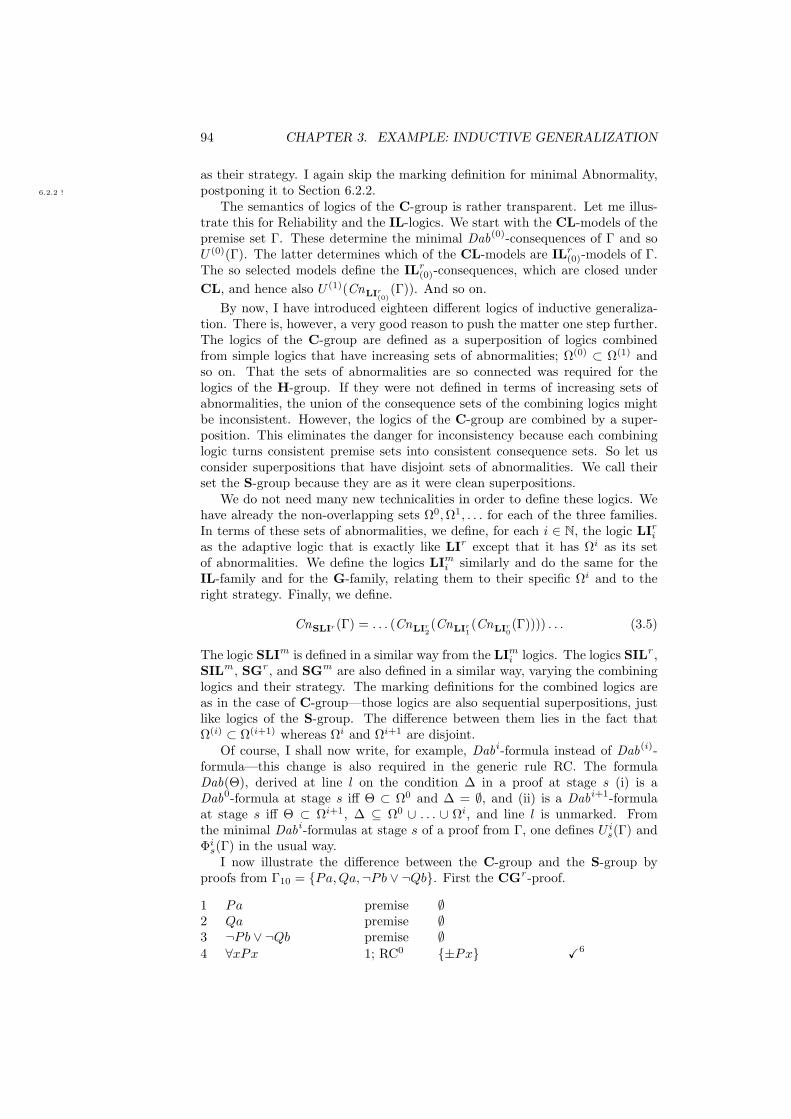
94 CHAPTER 3. EXAMPLE: INDUCTIVE GENERALIZATION
as their strategy. I again skip the marking definition for minimal Abnormality,postponing it to Section 6.2.2.6.2.2 !
The semantics of logics of the C-group is rather transparent. Let me illus-trate this for Reliability and the IL-logics. We start with the CL-models of thepremise set Γ. These determine the minimal Dab(0)-consequences of Γ and soU (0)(Γ). The latter determines which of the CL-models are ILr
(0)-models of Γ.The so selected models define the ILr
(0)-consequences, which are closed underCL, and hence also U (1)(CnLIr(0)
(Γ)). And so on.By now, I have introduced eighteen different logics of inductive generaliza-
tion. There is, however, a very good reason to push the matter one step further.The logics of the C-group are defined as a superposition of logics combinedfrom simple logics that have increasing sets of abnormalities; Ω(0) ⊂ Ω(1) andso on. That the sets of abnormalities are so connected was required for thelogics of the H-group. If they were not defined in terms of increasing sets ofabnormalities, the union of the consequence sets of the combining logics mightbe inconsistent. However, the logics of the C-group are combined by a super-position. This eliminates the danger for inconsistency because each combininglogic turns consistent premise sets into consistent consequence sets. So let usconsider superpositions that have disjoint sets of abnormalities. We call theirset the S-group because they are as it were clean superpositions.
We do not need many new technicalities in order to define these logics. Wehave already the non-overlapping sets Ω0, Ω1, . . . for each of the three families.In terms of these sets of abnormalities, we define, for each i ∈ N, the logic LIr
i
as the adaptive logic that is exactly like LIr except that it has Ωi as its setof abnormalities. We define the logics LIm
i similarly and do the same for theIL-family and for the G-family, relating them to their specific Ωi and to theright strategy. Finally, we define.
CnSLIr (Γ) = . . . (CnLIr2(CnLIr1
(CnLIr0(Γ)))) . . . (3.5)
The logic SLIm is defined in a similar way from the LImi logics. The logics SILr ,
SILm , SGr , and SGm are also defined in a similar way, varying the combininglogics and their strategy. The marking definitions for the combined logics areas in the case of C-group—those logics are also sequential superpositions, justlike logics of the S-group. The difference between them lies in the fact thatΩ(i) ⊂ Ω(i+1) whereas Ωi and Ωi+1 are disjoint.
Of course, I shall now write, for example, Dabi-formula instead of Dab(i)-formula—this change is also required in the generic rule RC. The formulaDab(Θ), derived at line l on the condition ∆ in a proof at stage s (i) is aDab0-formula at stage s iff Θ ⊂ Ω0 and ∆ = ∅, and (ii) is a Dabi+1-formulaat stage s iff Θ ⊂ Ωi+1, ∆ ⊆ Ω0 ∪ . . . ∪ Ωi, and line l is unmarked. Fromthe minimal Dabi-formulas at stage s of a proof from Γ, one defines U i
s(Γ) andΦi
s(Γ) in the usual way.I now illustrate the difference between the C-group and the S-group by
proofs from Γ10 = Pa,Qa,¬Pb ∨ ¬Qb. First the CGr -proof.
1 Pa premise ∅2 Qa premise ∅3 ¬Pb ∨ ¬Qb premise ∅4 ∀xPx 1; RC0 ±Px X6

3.5. COMBINED ADAPTIVE LOGICS 95
5 ∀xQx 2; RC0 ±Qx X6
6 ±Px ∨ ±Qx 1, 2, 3; RU ∅7 ∀x(Px ⊃ Qx) 1, 2; RC1 Px ∧ ±Qx X9
8 ∀x(Qx ⊃ Px) 1, 2; RC1 Qx ∧ ±Px X11
9 ±Px ∨ (Px ∧ ±Qx) 1, 2, 3; RU ∅10 Px ∧ ±Qx 9; RC0 ±Px X6
11 ±Qx ∨ (Qx ∧ ±Px) 1, 2, 3; RU ∅Remember the marking definition. We first mark for degree 0. This meansthat the marks with superscript 6 are added. So ±Px ∨ (Px ∧ ±Qx) and±Qx ∨ (Qx ∧ ±Px) are minimal Dab(1)-formulas, whence lines 7 and 8 aremarked.
Line 10 is only inserted to illustrate that ±Px ∨ (Px ∧ ±Qx) is a minimalDab1-consequence of Γ10 whereas Px∧±Qx is not (because line 10 is marked).
Next consider the SGr -proof, in which I do not repeat the premises.
4 ∀xPx 1; RC0 ±Px X6
5 ∀xQx 2; RC0 ±Qx X6
6 ±Px ∨ ±Qx 1, 2, 3; RU ∅7 ∀x(Px ⊃ Qx) 1, 2; RC1 Px ∧ ±Qx8 ∀x(Qx ⊃ Px) 1, 2; RC1 Qx ∧ ±Px9 ±Px ∨ (Px ∧ ±Qx) 1, 2, 3; RU ∅10 Px ∧ ±Qx 1, 5; RU ±Px X6
11 ±Qx ∨ (Qx ∧ ±Px) 1, 2, 3; RU ∅
The same lines are still marked in view of ±Px∨±Qx, which is a minimal Dab0-formula. However, ±Px ∨ (Px ∧ ±Qx) and ±Qx ∨ (Qx ∧ ±Px) are not Dab1-formulas because ±Px and ±Qx are not members of Ω1. Moreover, Px∧±Qx isnot a Dab1-formula either because line 10 is marked. The fact that Gr
1 has Ω1 asits set of abnormalities, rather than Ω(1), causes lines 7 and 8 to be unmarkedat stage 10 and actually causes ∀x(Px ⊃ Qx) and ∀x(Qx ⊃ Px) to be finalSGr -consequences of Γ10.
A warning has to be issued with respect to strategies. Where simple adap-tive logics were considered, the Minimal Abnormality strategy always offers aricher consequence set than Reliability. This does not hold for combined adap-tive logics that are sequential superpositions of simple adaptive logics. If the‘innermost’ simple adaptive logic has Minimal Abnormality as its strategy, itmay have a larger consequence set than its variant that has Reliability as itsstrategy. This larger consequence set may contain Dab-formulas of the nextinnermost simple adaptive logic. Some of these may not be derivable by theReliability strategy.31 So the strengthening of the innermost logic may causethe consequence set of the next innermost logic to be weaker. A simple example(with thanks to Mathieu Beirlaen) is offered by a premise set we have alreadyseen: Γ10 = Pa, Qa,¬Pb∨¬Qb. The SGm -consequence set of Γ10 is identical
31In Chapter 5 I shall prove Theorem 5.6.2, which states that the derivable Dab-formulasare determined by the lower limit logic only. This might confuse the reader who wouldreturn to the present chapter. The explanation is simple: every combining logic adds certaingeneralizations to its consequence set. This consequence set, say S, is the premise set of thenext combining adaptive logic, but is also closed under CL. Note that S may very well containDab-formulas (of the next combining logic) that are not derivable from the previous premiseset.

96 CHAPTER 3. EXAMPLE: INDUCTIVE GENERALIZATION
to the CL-consequence set of Γ10∪∀xPx∨∀xQx. This contains, for example,Pb∨Qb, and hence also (Pb∧¬Qb)∨(¬Pb∧Qb). The SGr -consequence set of Γ10
is identical to the CL-consequence set of Γ10 ∪ ∀x(Px ⊃ Qx), ∀x(Qx ⊃ Px).This contains, for example, ¬Pb ∧ ¬Qb. I shall consider the proofs in Section6.2.3.Section 6.2.3 nazien
This illustrates the difference between SGm and SGr and shows that theirconsequence sets are incommensurable for this premise set. SGm squeezes outmore at the level of the most general hypotheses, but what one obtains is onlya disjunction of generalizations as well as disjunctive predictions, even on theobject b. SGr proceeds more carefully, delivers nothing at all concerning gen-eralizations of degree 0, but delivers more concerning generalizations of degree1. Even very weak extensions of the premise set cause SGm and SGr to agree.That is not surprising. Adding a sufficient amount of new data will cause allour logics of inductive generalization to agree, as they should.
It seems wise to insert a table listing the 24 logics of inductive generalizationthat we met.
LI-family IL-family G-familysimple LIr LIm ILr ILm Gr Gm
H-group HLIr HLIm HILr HILm HGr HGm
C-group CLIr CLIm CILr CILm CGr CGm
S-group SLIr SLIm SILr SILm SGr SGm
The reader became acquainted with ampliative adaptive logics as well aswith three kinds of combined adaptive logics. Meanwhile, I have shown thatthere is a large variety of logics of inductive generalization. Some readers mightthink that one should simply apply the strongest logic of this set, but this is notalways the right choice. It is for example possible that the final consequencesassigned to a data set by a combined logic are generalizations of a low degree, ordisjunctions of them, whereas the final consequences assigned to the same dataset by the corresponding simple logic comprises more interesting generalizationsof a higher degree. Much will depend on the knowledge or presumptions aresearcher has about a certain domain. Much will also depend on whether theaim of the application is to act on the basis of a prediction, in which case it iswise to be careful, or to set up a set of interesting experiments in view of thepresent data, in which case very general hypotheses will soon be shown false iffalse they are.
Before moving on to background knowledge, let me answer a possible com-plaint. Some people will wonder whether all these logics have any use. Theymight argue that Reichenbach’s Straight Rule from [Rei38] even provides amethod for deriving probabilistic hypotheses and so can be downgraded to ap-ply to inductive generalizations as considered here. The idea is that one takesone’s past experiential data as representative for all possible data. In otherwords, one takes the universe to be constituted by facts that are similar tothose experienced. One takes them to occur in the universe with the frequen-cies that are present in our past experience, a matter disregarded in this chapter.As Reichenbach argued, in the end the Straight Rule leads to success if it is pos-sible to obtain success. So are the adaptive logics of inductive generalizationnot a useless complication?
Obviously, I would not have written this chapter if I did not think to have

3.6. HANDLING BACKGROUND KNOWLEDGE 97
an answer to that complaint. Go over all the premise sets introduced in thischapter. To almost none of them can the Straight Rule be applied. The StraightRule can be applied if all properties of all observed objects are known. It canbe applied, although a supplementary rule is then involved, if there is a setof objects of which all properties are known and every other observed objecthas properties that are a subset of the properties in the first set. The involvedsupplementary rule is that every partially known object agrees with a fullyknown object. Most premise sets we considered in this chapter require a morecomplex reasoning.
Where those restrictions are met, all adaptive logics introduced in this chap-ter lead to exactly the same result as the Straight Rule. To prove this is a bittedious, but the following insights help. In so restricted cases, the derivableDab-formulas have, for all twenty-four logics, one disjunct only. If that is so,Reliability and Minimal Abnormality lead to the same result. Next, it is notdifficult to see that, if the known objects are completely described, the simpleadaptive logics of the three families classify the same generalizations either asderivable at a stage and unmarked in all extensions or as not derivable at astage or marked in an extension. Finally, if the known objects are completelydescribed, none of the combined logics can offer anything more than the simplelogic on which it is based. So, indeed, the adaptive logics of this chapter differfrom each other only for premise sets that do not meet the restrictions.
So the question is whether premise sets that do not meet the restrictions areinteresting. Needless to say, premise sets that meet the restrictions are neveravailable as such. They are only obtained if it is determined beforehand whichproperties are qualified as relevant, if the set of these properties is sufficientlysmall, and if the properties in this set are easily observable, either as such orby performing certain experiments. Deciding beforehand which properties arequalified as relevant is the tricky matter here. One may be lucky by selecting, onthe basis of background knowledge or of a worldview, a set of ‘easily’ observableproperties that display a regularity. Whenever this is not the case, however, oneneeds the possibility to broaden one’s scope. In order to do so, one needs to beable to assess which other properties might play a role. The Straight Rule hasnothing to offer in this respect.
3.6 Handling Background Knowledge
The easiest way to handle background knowledge is by adding it to the availabledata, in other words to the premise set. Two problems lurk around the cornerthough. The first is that the background knowledge may be inconsistent, thesecond that it is falsified by the data. As this chapter is written from a classicoutlook, I shall largely disregard the first problem. Tackling it is beyond thescope of a chapter that is meant to introduce ampliative as well as combinedadaptive logics, but the reader will nose, in view of the previous chapter, inwhich way the problem should be tackled.
The possibility of falsification obviously cannot be neglected even within afully classical framework—no classical logician could locate anything deviant inPopper’s work. The trouble is that Popper’s advice to discard falsified theoriesis too simple. For more than thirty years—I mean [Lau77]—everyone who canread and has access to the literature should know that scientists often continue

98 CHAPTER 3. EXAMPLE: INDUCTIVE GENERALIZATION
to reason from falsified theories. They typically consider the falsifications asproblems but keep relying on other consequences of the falsified theory. Inother words, discarding falsified theories is not always a good advice because itwould leave one without any information about the domain.
It follows that two different cases need to be distinguished: those in whichwe discard a falsified theory altogether and those in which we only discard thefalsified consequences of the theory. In the first case, I shall say that one handlesthe theories strictly, in the second case that one handles them pragmatically.Note that a falsification may only be discovered after some reasoning. So weare in defeasible waters here.
A further distinction has to be made. Part of our background knowledgeconsists of separate statements whereas other parts are theories—for presentpurposes, any non-singleton set of statements will be considered to be a theory.Handling theories, whether strictly or pragmatically, will turn out to be a triflemore difficult than handling separate statements.
The picture is not complete yet. That the data falsify a piece of backgroundknowledge is the simple case. More often, however, the data falsify a set ofbackground knowledge without falsifying any single theory or any single separatestatement in the set. In such cases, it is important to take into account thatelements of our background knowledge may differ in plausibility. One will rejectthe piece of background knowledge that is least plausible anyway. So we needplausibilities or priorities or preferences—I shall take these words to have thesame meaning in the present context. Incidentally, this makes the matter evenmore defeasible. With all this in mind, let us go for it.
Priorities will be expressed within the object language. This has two advan-tages over the layered tuples of premises that are popular with some computerscientists. The tuples have the form 〈Γ0,Γ1, . . . , Γn〉 in which32 Γ0 comprisesthe certainties (the so-called real premises), Γ1 comprises the very plausiblestatements, Γ2 the less plausible statements, and so on up to Γn. The firstadvantage of expressing the priorities in the object language is that we have tohandle a single premise set instead of a tuple. The second advantage is that itresults in a richer framework. It enables one, for example, to express that eitherA has plausibility 1 or B has plausibility 2.
Priorities will be expressed by one or more symbols ¦ if they pertain tostatements and theories that are handled strictly and by one or more symbols ♦if they pertain to entities that are handled pragmatically. Let A be a statementof the predicative language. That A, in which no diamond occurs, is a premisemeans that A belongs to the data, to which certainty is attached. That ♦A,respectively ¦A, is a premise will express that A has the highest priority lowerthan certainty. That ♦♦A, respectively ¦ ¦A, is a premise expresses that A hasthe next highest priority, and so on. To simplify the notation, I shall write ♦nA,respectively ¦nA, to abbreviate A preceded by n diamonds (of the same sort).
Let me at once mention the way to handle a theory T = 〈Γ,CL〉 that haspriority n—given the context, I suppose that all theories are closed under CL.To handle T , we let ♦n(A1 ∧A2 ∧ . . . ∧Ak) | k ≥ 1;A1, A2, . . . , Ak ∈ Γn be asubset of the premise set; similarly for ¦ if the theory is handled strictly. If Γis a finite set of statements, we may just as well put all of these in conjunction
32The Γi in this expression have obviously nothing to do with the Γi I use elsewhere in thischapter to denote specific premise sets.

3.6. HANDLING BACKGROUND KNOWLEDGE 99
and prefix ♦n or ¦n to this conjunction.In order to avoid very complex systems in this introductory chapter, I shall
presuppose that all pieces of background knowledge, whether separate state-ments or theories, have a distinct priority. This unrealistic restriction will beremoved in Section 6.2.2. At any point in time, there will be at most finitelymany pieces of background knowledge. By the simplification just introducedeach of them has a specific priority, which is different from the priority of allother pieces of background knowledge. It follows that only finitely many prior-ities are involved. This completes the description of premise sets that containbackground knowledge.
Let us move on to the adaptive logics that handle the priorities. The under-lying idea of these logics is to add to the certainties first as much as possible ofthe highest priority level; to the result of this one adds as much as possible ofthe next priority level; and so on. From a technical point of view we upgradethe standard language to a modal one by adding the symbols ♦ and ¦. Themeaning of the modalities is fixed by a modal logic: a predicative version of thelogic K. The semantic metalanguage will contain the set of pseudo-constantsO—see Chapter 1 for the reasons to do so. Let WmO denote the set of wffs ofthe modal pseudo-language LmO.
A K-model M is a quintuple 〈W,w0,R, D, v〉 in which W is a set of worlds,w0 ∈ W , R is a binary relation on W , D a non-empty set and v an assignmentfunction. The assignment function v is as follows:33
C1.1 v : WO ×W → 0, 1C1.2 v : C ∪ O ×W → D (where D = v(α, w) | α ∈ C ∪ O; w ∈ W)C1.3 v : Pr ×W → ℘(Dr)
The valuation function, vM : WmO ×W → 0, 1, determined by the model Mis defined by:
C2.1 where A ∈ S, vM (A,w) = v(A, w)C2.2 vM (πrα1 . . . αr, w) = 1 iff 〈v(α1, w), . . . , v(αr, w)〉 ∈ v(πr, w)C2.3 vM (α = β, w) = 1 iff v(α, w) = v(β,w)C2.4 vM (¬A,w) = 1 iff vM (A,w) = 0C2.5 vM (A ∨B, w) = 1 iff vM (A,w) = 1 or vM (B, w) = 1C2.6 vM ((∃α)A(α), w) = 1 iff vM (A(β), w) = 1 for at least one β ∈ C ∪ OC2.7 vM (♦A,w) = 1 iff vM (A,w′) = 1 for at least one w′ such that Rww′.C2.8 vM (¦A,w) = 1 iff vM (A,w′) = 1 for at least one w′ such that Rww′.
All other logical symbols are explicitly defined in the usual way. A K-model Mverifies A ∈ Wm, abbreviated as M ° A, iff vM (A,w0) = 1. Γ ²K A (A is asemantic consequence of Γ) iff all K-models of Γ verify A. ²K A (A is K-valid)iff A is verified by all K-models.34
33I refer to the CL-semantics for the justification of the peculiarities of the semantic format.34For those familiar with modal logics, a bit of explanation seems useful to relate the style of
the semantics to different styles. One may define a function d that assigns to each w ∈ W itsdomain d(w) = v(α, w) | α ∈ C ∪O. If an element of an r-tuple of v(πr, w) does not belongto d(w), then the r-tuple does not have any effect on the valuation. So v(πr, w) ∈ ℘(d(w)r)”.Note that, if Rww′, the question whether v(α, w) is or is not a member of d(w′) is immaterialfor the value of vM (A, w). For example, the value of vM (♦Pa, w) is determined by the valuesof v(a, w′) and v(P, w′) for those w′ for which Rww′. The semantics may be rephrased asa counterpart semantics: a ∈ d(w) is a counterpart of b ∈ d(w′) just in case there is anα ∈ C ∪ O such that v(α, w) = a and v(α, w′) = b. An α ∈ C ∪ O may be seen as picking aspecific counterpart ‘path’ on W .

100 CHAPTER 3. EXAMPLE: INDUCTIVE GENERALIZATION
This seems the best point to add some comments on reading of the diamondsas expressing plausibility. The symbols ♦ and ¦ have exactly the same meaningin K. We nevertheless need both of them because they will be handled differentlyby the adaptive logics.
Some people are confused about the meaning of ¬♦¬A—the other may skipthe rest of this paragraph. The confusion is caused by the failure to distinguishbetween (i) “A is plausible” is not derivable from a given premise set and (ii) “Ais not plausible” is derivable from a given premise set. Put differently and interms of an example, ♦p is false in some models of q, ♦r, and so is not asemantic consequence of q, ♦r, but ♦p is true in other models of the premiseset, whence ¬♦p is not a semantic consequence of the premise set either. Notealso that ¬♦2A excludes neither A nor ♦iA for i 6= 2. In other words, that Ais not plausible to degree 2 does not exclude that it is true, or plausible to anyother degree.
To avoid unnecessary complications, I shall not spell out the proof theoryof the modal logic K but suppose that it is available. So let us turn to theadaptive logic that handles background knowledge in the desired way. It will bea combined adaptive logic, just like the logics from the C-group and the S-groupin Section 3.5. As the reader is already familiar with combined adaptive logics,I shall first present the logic and only thereafter discuss an example of a proof.
What counts as an abnormality is that a formula is plausible (to some degree)and nevertheless false. We have to take two kinds of priorities into account. Irecall that ¦ refers to the strict handling of background knowledge and ♦ to thepragmatic handling. Moreover, that something plausible is false is worse as itis more plausible. So we define a sequence of sets of abnormalities, for everyi ≥ 1,
Ωi = ∃(♦iA ∧ ¬A) | A ∈ A ∪ ∃(¦iB ∧ ¬B) | B ∈ Ws ,
in which A is the set of (non-modal) atoms from the second paragraph of Sectionplaats nazien
3.4. There is a very good reason for there to be two kinds of abnormalities. Thiswill become clear in a few paragraphs.
The logic K is combined with the sets of abnormalities and with the Reli-ability strategy, into an infinite sequence of simple adaptive logics Kr
i (i ≥ 1).Finally, we combine all simple Kr
i into Kr by a sequential superposition—notethe analogy with the definition of SGr .
CnKr (Γ) = . . . (CnKr3(CnKr
2(CnKr
1(Γ)))) . . . (3.6)
As the weakest priority will be represented by a finite number of diamonds inany premise set, Kr reduces to the combination of finitely many combininglogics in every application. I leave it to the reader to define the combined logicKm similarly.
The dynamic Kr -proofs (and Km -proofs) are defined by rules and a markingdefinition. The rules are exactly like those of the logics of the S-group in theprevious section. As was the case there, the rules of all combining logics maybe applied in any order in Kr -proofs.
Other things are also similar to Section 3.5. I shall write RCi in proofs, thusreferring to the specific logic Kr
i to which the rule belongs. The conditions ofthe formulas A1, . . . , An in RU as well as in RC may contain abnormalitiesfrom any Ωj and actually from several Ωj . The full conditions are carried overby those rules to the condition of B, as the rules indicate.

3.6. HANDLING BACKGROUND KNOWLEDGE 101
The marking definition is identical to Definition 3.5.3 but some parametersshould be adjusted. A disjunction of members of (the present) Ωi that is theformula of a line of a proof counts as a Dabi-formula iff it is derived on acondition ∆ ⊆ Ω1 ∪ . . . ∪ Ωi−1. U i
s(Γ) comprises the disjuncts of the minimalDabi-formulas at stage s of a proof. The only difference between Definition3.5.3 and the subsequent one is that we start from i = 1 and that i ≥ 1 in thesuperscript of U i
s(Γ).35
Definition 3.6.1 Marking for Reliability: Starting from i = 1, a line is i-marked at stage s iff, where ∆ is its condition, ∆ ∩ U i
s(Γ) 6= ∅.The marking definition for Minimal Abnormality is once more postponed plaats “once more”
to Chapter 6. So we go straight to the combination of the logic that handlesbackground knowledge with the one that inductively derives generalizations.It is easy to see which combination is needed. Where L is the logic handlinginductive generalization and the set of data and background knowledge is closedunder Kr , the desired combination is CnL(CnKr (Γ)).
Let us move to an example. Toy examples are obviously bound to beartificial. Let the data be Pa,¬Qa,¬Pb, Qc,Rc,¬Qd, let the backgroundknowledge comprise (i) a theory T1 = ∀x(Px ⊃ Rx),∀x(Rx ⊃ ¬Qx) that ishandled strictly and has priority 1 (single diamond), (ii) a singular statement∀x(Px ⊃ Qx) that is handled pragmatically and has priority 2, and (iii) a sin-gular statement ∀x(Rx ⊃ Px) that is handled strictly and has priority 3. Sothe premise set will comprise the nine formulas displayed in the following proof:
1 Pa premise ∅2 ¬Qa premise ∅3 ¬Pb premise ∅4 Qc premise ∅5 Rc premise ∅6 ¬Qd premise ∅7 ¦∀x(Px ⊃ Rx) premise ∅8 ¦∀x(Rx ⊃ ¬Qx) premise ∅9 ¦(∀x(Px ⊃ Rx) ∧ ∀x(Rx ⊃ ¬Qx)) premise ∅10 ♦2∀x(Px ⊃ Qx) premise ∅11 ¦3∀x(Rx ⊃ Px) premise ∅
As the only theory comprises finitely many non-logical axioms, it is suffi-cient to list the conjunction of these axioms preceded by the right number ofdiamonds. So lines 7 and 8 are obviously redundant.
Let us first see what becomes of T1. To keep the proof within the margins,?♦iA will abbreviate ∃(♦iA ∧ ¬A) and similarly for ¦.12 ∀x(Px ⊃ Rx) 7; RC1 ?¦∀x(Px ⊃ Rx)13 ∀x(Rx ⊃ ¬Qx) 8; RC1 ?¦∀x(Rx ⊃ ¬Qx)14 ∀x(Px ⊃ Rx) ∧ ∀x(Rx ⊃ ¬Qx) 9; RC1
?¦(∀x(Px ⊃ Rx) ∧ ∀x(Rx ⊃ ¬Qx))Each of the three derived formulas may be derived on different conditions aswell. Doing so or deriving other formulas from 7–9 by RC is rather pointless
35The reason for the difference is that Ω0 was not defined in the present context, viz. fiveparagraphs ago in the text.

102 CHAPTER 3. EXAMPLE: INDUCTIVE GENERALIZATION
because all of them will be marked. Theory T1 is obviously falsified by Rc andQc. So one may continue as follows.
15 ¬∀x(Rx ⊃ ¬Qx) 4, 5; RU ∅16 ?¦∀x(Rx ⊃ ¬Qx) 8, 15; RU ∅At stage 16, line 13 is marked and will remain marked forever. It is easily seenthat ?¦1(∀x(Px ⊃ Rx) ∧ ∀x(Rx ⊃ ¬Qx)) is derivable from 9 and 15. As soonas it is derived, line 14 is marked and will remain marked forever.
What about line 13 and what about other lines that may be added to theproof and at which formulas are derived from T1? The answer is very simple:they will all be marked. They all have a condition that comprises a formula ofthe form ¦1A ∧ ¬A and all such formulas are provably unreliable. This is asdesired. We wanted to handle T1 in a strict way: either all of it is added to thedata, in case T1 is compatible with the data, or all of it is discarded, in case thedata contradict T1. The strict handling is realized by devising Kr as a flip-floplogic with respect to the modality ¦.
So let me show that Kr is a flip-flop with respect to the modality ¦ and thatthis results in the strict handling of formulas and theories qualified with thatmodality. Note, first of all, that the discussion concerns a specific composinglogic of Kr , namely Kr
1. So let us concentrate on this. If no Dab1-formula is K-derivable from the premises, no line with a condition ∆ ⊂ Ω1 will be marked. Sothe Kr
1-consequences of the premise set coincide with the consequences deliveredby the upper limit logic, which is Triv. So I have to show that, if a Dab1-formulais K-derivable from the premises, then the Kr
1-consequences of the premise setcoincide with the consequences delivered by the lower limit logic, which is K.
Consider a proof in which a Dab1-formula has been derived, say
(¦A1 ∧ ¬A1) ∨ . . . ∨ (¦An ∧ ¬An) , (3.7)
and in which occurs a line at which B is derived by RC1 on the condition ∆ ⊆ Ω1
from a formula of a line with the empty condition. As B is derivable on thecondition ∆ from the premise set,
B ∨Dab1(∆)
is a K-consequence of the premise set.36 From this and (3.7) follows, by propo-sitional CL:
(¦A1 ∧ (¬A1 ∧B)) ∨ . . . ∨ (¦An ∧ (¬An ∧B)) ∨Dab1(∆)
and from this, again by propositional CL:
(¦A1 ∧ ¬(A1 ∨ ¬B)) ∨ . . . ∨ (¦An ∧ ¬(An ∨ ¬B)) ∨Dab1(∆) .
From this, as ¦Ai `K ¦(Ai ∨ ¬B), follows:
(¦(A1∨¬B)∧¬(A1∨¬B))∨ . . .∨(¦(An∨¬B)∧¬(An∨¬B))∨Dab1(∆) . (3.8)
If (3.8) is a minimal Dab1-consequence of the premise set Γ, then ∆ ⊆ U1(Γ).Suppose then that (3.8) is not a minimal Dab1-consequence of Γ. So there is a
36This is proved as Lemma 4.4.1.

3.6. HANDLING BACKGROUND KNOWLEDGE 103
minimal Dab1-consequence D of Γ which contains some but not all disjuncts of(3.8). If some members of ∆ are a disjunct of D, then ∆ ∩ U1(Γ) 6= ∅. If nomember of ∆ is a disjunct of D, then B is K-derivable from the premise set.37
What we learned is that, in the example proof we are constructing, everyline that has a condition of the form ¦C ∧ ¬C will be marked once the rightDab1-formulas have been derived (and I have shown the way in which such Dab1-formulas may be constructed). So let us not derive any further formulas fromT1, but move on to ♦2∀x(Px ⊃ Qx). Of course, the generalization ∀x(Px ⊃ Qx)is also falsified by the data, but it is handled pragmatically and this is what Iwant to illustrate now.
17 ∀x(Px ⊃ Qx) 10; RC2 ?♦2∀x(Px ⊃ Qx) X18
18 ?♦2∀x(Px ⊃ Qx) 1, 2, 10; RU ∅19 ♦2(Pd ⊃ Qd) 10; RU ∅20 Pd ⊃ Qd 19; RC2 ?♦2(Pd ⊃ Qd)21 ¬Pd 6, 20; RU ?♦2(Pd ⊃ Qd)
So notwithstanding the presence of Pa and ¬Qa, which jointly falsify ∀x(Px ⊃Qx), one may derive a consequence of ♦2∀x(Px ⊃ Qx), for example 19, andobtain a diamond-free formula from this on its ‘own’ condition, in the exam-ple ?♦2(Pd ⊃ Qd). This illustrates nicely what pragmatic handling comes to:a plausible background statement (or theory) is falsified, but one neverthelessrelies on non-falsified consequences of it.
The reader may wonder whether the derivability of the abnormality 19 doesnot result in U2(Γ) = Ω2—compare this to the fact that I showed that U1(Γ) =Ω1. Well, while Kr is a flip-flop with respect to the modality ¦, it is not withrespect to the modality ♦. I cannot prove this at this point, but I can indicatewhere the difference stems from. If the symbol ¦ in (3.8) is replaced by thesymbol ♦, the result is not a Dab-formula any more—please check again theway in which the Ωi are defined (some three pages before this one). Note alsothat the difference is related to the distinct way in which the diamonds occurin the Ωi, not to the difference in number of diamonds. Tr is a flip-flop withrespect to ¦2 just as much as with respect to ¦, but not with respect to any ♦i.
Finally consider ¦3∀x(Rx ⊃ Px). The involved generalization is not falsifiedby the data extended with non-falsified consequences of ∀x(Px ⊃ Qx). Sothings will proceed smoothly.
22 ∀x(Rx ⊃ Px) 11; RC3 ?¦3∀x(Rx ⊃ Px)23 ¬Rb 3, 22; RU ?¦3∀x(Rx ⊃ Px)24 Pc 5, 22; RU ?¦3∀x(Rx ⊃ Px)25 Pd ∨ ¬Rd 22; RU ?¦3∀x(Rx ⊃ Px)26 ¬Rd 21, 25; RU ?♦2(Pd ⊃ Qd), ?¦3∀x(Rx ⊃ Px)
All formulas derived at the unmarked lines 18–26 are finally derivable fromthe premise set (1–11). Of course, we are not home yet. We only derived theuseful consequences of the premise set (data plus plausible background knowl-edge). To this result, we now should apply a logic of inductive generalization.If this logic is Gr , we want the following combined consequence set.
CnGr (CnKr (Γ)) (3.9)37It is then derivable by propositional CL from every disjunct of D. Indeed, all of these
have the form ¦(Ai ∨ ¬B) ∧ ¬(Ai ∨ ¬B), which is equivalent to ¦(Ai ∨ ¬B) ∧ ¬Ai ∧B.

104 CHAPTER 3. EXAMPLE: INDUCTIVE GENERALIZATION
In other words, we first upgrade the data with the background knowledge andthen apply the logic of inductive generalization to this. In order to do so, wesimply continue within the same proof. Moreover, we may apply the rules allinvolved logics at any point in the proof. The marking definition is obvious. Itis identical to Definition 3.6.1, except that, after the lines have been marked forall the logics combined into Tr , they are marked in view of Gr . Please checkthat, for any premise set, the marking definition leads only to finitely many‘rounds’ of marking and that this remains so if the simple adaptive logic Gr isreplaced, for example by the combined SGr .
Before moving on to the next section, let me make sure that the reader keepsin mind the way in which Dab-formulas are defined in the context of the lastexample proof. Remember that Dab1-formulas are disjunctions of members ofΩ1, which is the ‘innermost’ or ‘lowest’ set of abnormalities in this case. Dab2-formulas are disjunctions of members of Ω2 that are derived at an unmarked lineon a condition that is a subset of Ω1. In the example proof, the only interestingDab2-formulas are derived on the empty condition because, as we have seen, alllines that have members of Ω1 in their condition are marked as soon as the rightDab1-formulas are derived. Dab3-formulas are disjunctions of members of Ω3
that are derived at an unmarked line on a condition that is a subset of Ω1∪Ω2. Inthe example proof, no Dab3-formulas are derivable, which means that ∀x(Rx ⊃Px) is not falsified by the data extended with non-falsified consequences of∀x(Px ⊃ Qx). As a result of all this, the logic of inductive generalization is notapplied to the original set of data, which is Pa,¬Qa,¬Pb, Qc, Rc,¬Qd, butto Pa,¬Qa,¬Pb,¬Rb, Pc,Qc, Rc,¬Pd,¬Qd,¬Rd.38
I do not claim that this enriched set will lead to more generalizations than theoriginal data set. One takes background knowledge into account not because onewants to obtain a richer set of generalizations, but because one wants to buildupon the theoretical insights (empirical generalizations and theories) gained byprevious generations. This obviously cannot be illustrated by toy examples. Noris the mechanism suitable in the case of toy examples. The mechanism is onlysuitable because we have a vast set of data, pertaining to a vast set of predicates.Background knowledge gives one a way to systematize these data, even if someof the generalizations and theories require exceptions, viz. pragmatic handling.Not relying on background knowledge leaves one with a mess of unstructureddata. This theme is continued in the next section.
Some readers may wonder that 24 logics of inductive generalization werepresented (and further ones are suggested), and only one logic to handle prior-itized background knowledge, which actually takes care of the strict as well asof the pragmatic handling of background knowledge. As announced I restrictedthe many ways in which background knowledge may be handled in order to keepthis introductory chapter as simple as possible.
3.7 Conjectures
Ampliative consequences derived by a logic of inductive generalization are jus-tified in view of a logical rationale, which is slightly different for every such
38Actually, much more effects of the background knowledge is present in the premise set towhich the logic of inductive generalization is applied, but these will have no effect on the newgeneralizations that will be derived.

3.7. CONJECTURES 105
logic. This rationale is fixed by the choice of the abnormalities and possibly byordering them in several sets and by the role these sets play in the combinedlogic. The derived generalizations are conjectures in the sense that the logicalrationale is not deduction. The logic is defeasible; it is also non-monotonic inthat the derived generalizations may be overruled by future data. In this sec-tion we shall deal with very different conjectures, for which there is at best anon-logical justification.
Suppose that, at some stage of a proof, A∨B ∨C is a minimal Dab-formula(at that stage), with A, B, and C abnormalities of the right kind. Each ofthe three abnormalities may prevent certain generalizations to be derivable. Aswe learn from Wisniewski’s erotetic logic, see for example [Wis95, Wis96], thedisjunction A∨B∨C invokes the question ?A, B,C, in words: Which of A, B,and C is the case? A full answer to this question might be A (or B or C), buteven ¬A (or ¬B or ¬C) would partially answer the question in that it reducesthe question to a simpler one.39
The effects of introducing ¬A in the proof are obvious: it enables one toderive B ∨ C. If A ∨ B ∨ C is the only Dab-formula in which A occurs, A willnot be a member of Us(Γ) if B ∨C is derived at stage s. So certain lines, whichwere marked at previous stages in view of the Dab-formula A ∨ B ∨ C, willbe unmarked at stage s of the proof. Put differently, by stating that certainabnormalities are false—remember that we are in a classical context—certaingeneralizations will become finally derivable.
If the person constructing the proof is not clumsy, ¬A is not derivable fromthe data. There may be several reasons for introducing ¬A. These reasons mayrelate to the state of the discipline, it may also relate to a world-view or to ametaphysical theory one subscribes to. But precisely because ¬A is not derivedfrom the data, it should not be put on the same foot as the data. In other words,¬A should not be introduced as a certainty, but as a statement that is assigneda certain plausibility but may be defeated by (present or) future experience.
The technical handling of this is obvious. One introduces ¬A with therequired priority. In other words one introduces the premise ¦i¬A with thesuitable i and handles it in the same way as one handles a piece of backgroundknowledge.40 So we do not need any new logic in this connection.
The reader might still have the feeling that some hocus pocus is going on. Solet me explain the latter explicitly. Consider a proof that contains the followinglines, in which A, B, and C are abnormalities of the logic Gr and A∨B ∨C isa minimal Dab-formula.
...11 A ∨B ∨ C . . . ∅12 ¦¬A Prem ∅13 ¬A 12; RC ¦¬A ∧A14 B ∨ C 11, 13; Ru ¦¬A ∧A
The fact that A ∨ B ∨ C is a minimal Dab-formula of Gr cannot cause lines13 and 14 to be marked. For one thing, A is not a member of the condition
39In technical terms, ?A, B, C together with ¬A implies the question ?B, C.40The restriction that all pieces of background knowledge (and formulas denying a cer-
tain abnormality) have a different priority was introduced in the present chapter to avoidcomplications. As promised, the general case will be discussed in Chapter 6.

106 CHAPTER 3. EXAMPLE: INDUCTIVE GENERALIZATION
of these lines. It is a conjunct of a member and that cannot result in the linesbeing marked. Moreover, in view of (3.9), the marking definition first markswith respect to the Kr -abnormalities, and only thereafter with respect to theGr -abnormalities. So if lines 13 and 14 are unmarked in view of Kr , B ∨ Cis a Dab-formula of Gr . Incidentally, the only case in which these lines maybe marked is where not only ¦¬A but also ¦¬B and ¦¬C are premises, or alsowhere A is a disjunct of another Dab-formula (of Gr ) and, for every disjunct Dof this Dab-formula, ¦¬D is a premise.
In some cases, one will not introduce ¬A, but rather one of the abnormalities,in the example A, B, and C. Of course the abnormality will again be introducedwith a certain plausibility. The effect is clear. If, for example, B is introducedas plausible and B is derived on the condition ¦B ∧ ¬B on a line that isunmarked in view of Kr , then both A and C will not be members of Us(Γ)from that stage s on (unless when they are also disjuncts of different minimalDab-formulas).41 As a result, certain generalizations will become derivable.42
One of the reasons for introducing some of the abnormalities with a cer-tain plausibility may be the researcher’s judgement on the relevance of certainpredicates. Suppose that someone takes there to be a lawful relation betweenP , Q, and R and considers other predicates are irrelevant for this relation. Ifa minimal Dab-formula in a Gr -proof contains a disjunct Px ∧ ±Sx, whereasother disjuncts contain only the predicates judged relevant, then consideringPx ∧ ±Sx as plausible is a way to express the irrelevance of S with respect tothe relation sought.
That scientists introduce abnormalities or negations of abnormalities with acertain plausibility partly explains that different research traditions will comeup with different theories. Such premises obviously do not release one fromgathering new information and from testing the obtained generalizations. How-ever, they allow researchers to arrive at conjectures that may later be modified,refined, or rejected. The existence of different research traditions will take careof the required search for potential falsifiers.
3.8 Some Comments in Conclusion
Many new kinds of adaptive logics were introduced in the present chapter. Alllogics were ampliative and some were combined. In subsequent chapters, weshall see that all these logics may be organized in a systematic way and thattheir properties may be studied in a unified way. The aim of this and thepreceding chapter was to illustrate the logics and their use, not to study themin a decent way.
A different kind of comment concerns the application of the logics. Thereader might have obtained the wrong impression that background knowledge,and especially the kind of conjectures introduced in the previous section, enableone to obtain generalizations that do not rely on empirical information. Thisimpression is wrong and two different aspects of the matter have to be keptapart.
41Obviously the occurrence of Us(Γ) refers to the logic of inductive generalization which isapplied after Kr is applied.
42It is instructive to modify the last example proof to the present case, to see that thematter is fully perspicuous.

3.8. SOME COMMENTS IN CONCLUSION 107
The first aspect concerns the specific defeasible character of all logics pre-sented in this chapter: any conclusion may be overruled by future empiricalevidence. The situation was very different in the previous chapter. There weconsidered a given theory that turned out inconsistent. The only problem wasto interpret the theory as consistently as possible. In the present chapter, newdata are bound to come up. So there is the supplementary problem to make surethat our generalizations and theories will survive future experience. The onlyway to do so is to test them. Popper is right that one should in the first placeperform those tests that will most likely lead to falsifications of our hypotheses.
The very different second aspect is that one needs to formulate hypothesesbefore testing them, and that one should rely on one’s past experience in orderto formulate them. This is where data and background knowledge comes in,and were world-views may provide one with further means of selection.
In Section 3.3, I offered some comments on the way in which LIr may guideresearch. More may be said about this and it should obviously be extended tothe other logics of inductive generalization. Moreover, one should realize thatthe intended research is in the first place part of the second aspect mentioned inthe previous paragraph. Of course, thus suggested observations and experimentswill already provide one with data that may falsify the hypotheses arrived at sofar. This does not mean, however, that they will always take care of the firstaspect discussed two paragraphs ago. More often than not, further observationsand experiments will be needed in view of the obtained generalizations.
Some friends, for example Atocha Aliseda, wondered whether the logics pre-sented in the present chapter were able to explain that a single observation is suf-ficient to derive certain generalizations and to consider them as well-established,whereas a diversity of observations is required before other generalizations willbe considered as established. It seems obvious to me that this difference de-pends on background knowledge. However, it is difficult to phrase the matterin a first-order context and I promised myself to restrict to first-order languagesin the present book.

108 CHAPTER 3. EXAMPLE: INDUCTIVE GENERALIZATION