Example-based Plastic Deformation of Rigid...
48
Example-based Plastic Deformation of Rigid Bodies Tae-Woo Lee 2019.04.04 Computer Graphics @ Korea University Ben Jones (Denver Univ.) et al. SIGGRAPH 2016
Transcript of Example-based Plastic Deformation of Rigid...

Example-based PlasticDeformation of Rigid Bodies
Tae-Woo Lee
2019.04.04
Computer Graphics @ Korea University
Ben Jones (Denver Univ.) et al.SIGGRAPH 2016
Tae-Woo Lee | 2019-04-22| # 2Computer Graphics @ Korea University
Index
• Abstract
• Introduction
• Related Work
• Method
• Authoring Simulation Assets
• Results and Discussion

Abstract

Tae-Woo Lee | 2019-04-22| # 4Computer Graphics @ Korea University
Abstract
An example-based plasticity model based on linear blend skinning
Deformation
Artists author simulation objects using familiar tools

Introduction

Tae-Woo Lee | 2019-04-22| # 6Computer Graphics @ Korea University
Introduction
• Large-scale destruction scene is used in physics-based animation
• The materials in these scenes are often man-made,carefully engineered and designed to be nearly rigid
• During failure, man-made materials such as steel and concreteexhibit plastic deformation and fracture
• Most of the existing approaches are based on continuum theory

Tae-Woo Lee | 2019-04-22| # 7Computer Graphics @ Korea University
Non-continuum Method Example(1/2)
• “Transformer 2 – breaking buildings”[Criswell (Industrial Light&Magic.) et al. / SIGGRAPH Conference 2010]
In advance, the object is broken to pieces of geometryand then integrate it seamlessly

Tae-Woo Lee | 2019-04-22| # 8Computer Graphics @ Korea University
Non-continuum Method Example(1/2)
• “Real-time deformation and fracture in a game environment”[Parker and O’Brien (Pixelux Entertainment) / SCA 2009]
Replaces the underlying geometry when destructive events occur,employ finite state machines and to hide temporal discontinuities
Tae-Woo Lee | 2019-04-22| # 9Computer Graphics @ Korea University
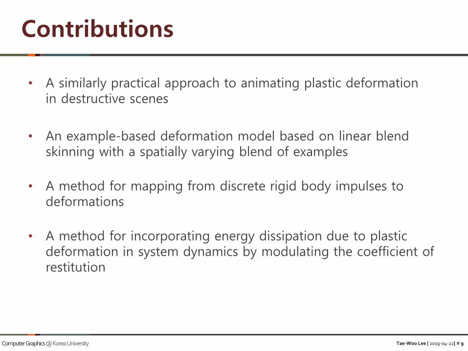
Contributions
• A similarly practical approach to animating plastic deformationin destructive scenes
• An example-based deformation model based on linear blend skinning with a spatially varying blend of examples
• A method for mapping from discrete rigid body impulses to deformations
• A method for incorporating energy dissipation due to plastic deformation in system dynamics by modulating the coefficient of restitution

Related Work

Tae-Woo Lee | 2019-04-22| # 11Computer Graphics @ Korea University
Related Work
Methods Based on Continuum Mechanics(1/2)
• Spring-mass system
“A peridynamic perspective on spring-mass fracture”[Levine (Clemson Univ.) et al. / SCA 2014]

Tae-Woo Lee | 2019-04-22| # 12Computer Graphics @ Korea University
Related Work
Methods Based on Continuum Mechanics(2/2)
• Lagrangian finite element method
“Simulating liquids and solid-liquid interactions withlagrangian meshes”[Clausen (California, Berkeley Univ.) et al. / SIGGRAPH 2013]

Tae-Woo Lee | 2019-04-22| # 13Computer Graphics @ Korea University
Related Work
Fracture Effect
• “Fracturing rigid materials”[Bao (Stanford Univ.) et al. / IEEE 2007]

Tae-Woo Lee | 2019-04-22| # 14Computer Graphics @ Korea University
Related Work
Denting and Bending
• “Efficient denting and bending of rigid bodies”[Patkar (Stanford Univ.) et al. / SCA 2014]

Tae-Woo Lee | 2019-04-22| # 15Computer Graphics @ Korea University
Related Work
Linear-Blend Skinning
• “Frame-based elastic models”[Gilles (British Columbia Univ.) et al. / SIGGRAPH 2011]

Tae-Woo Lee | 2019-04-22| # 16Computer Graphics @ Korea University
Related Work
Exampled-Based Simulation(1/2)
• “Drivenshape – a data-driven approach for shape deformation”[Kim and Vendrovsky (Rhythm and Hues Studios) / SCA 2008]
• “Sensitivity-optimized rigging for example-basedreal-time clothing synthesis”[Wang (Hangzhou normal Univ.) et al. / SIGGRAPH 2014]

Tae-Woo Lee | 2019-04-22| # 17Computer Graphics @ Korea University
Related Work
Exampled-Based Simulation(2/2)
• “Real-time example-based elastic deformation”[Koyama (Tokyo Univ.) et al. / SCA 2012]

Method

Tae-Woo Lee | 2019-04-22| # 19Computer Graphics @ Korea University
Method Overview(1/2)
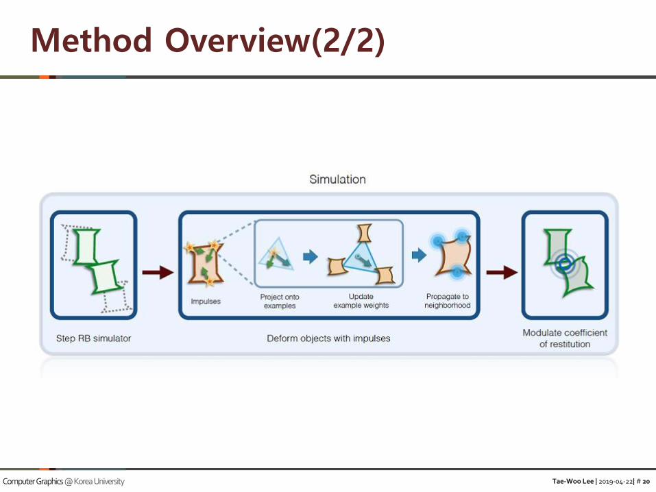
Tae-Woo Lee | 2019-04-22| # 20Computer Graphics @ Korea University
Method Overview(2/2)

Tae-Woo Lee | 2019-04-22| # 21Computer Graphics @ Korea University
Initial Setting(1/3)
• Artists begin by rigging their model with bones.
• Then, they use this rig to deform their input meshinto a set of characteristic example poses.
• Each object stores standard rigid body properties:
density, 𝜌, and mass, 𝓂 (both constant during simulation)
inertia tensor, 𝚰
linear position, x𝑐𝑜𝑚, and momentum p
orientation, 𝛀, and angular momentum, 𝐋
coefficient of restitution, 𝐶𝑟

Tae-Woo Lee | 2019-04-22| # 22Computer Graphics @ Korea University
Initial Setting(2/3)
• Geometry of object is modeled usinga tetrahedral mesh with 𝑁 vertices.
• The skinned vertex positions are determinedby the transformations of the 𝐵 bones.
• The user provides a set of 𝐸 example poses for the object,where each example contains a rotation and translationfor each bone.
Tae-Woo Lee | 2019-04-22| # 23Computer Graphics @ Korea University
Initial Setting(3/3)
• To track skinning properties over time, each object stores
undeformed mesh vertex positions, 𝐮 ∈ ℝ𝑁×3
skinned mesh vertex positions, x ∈ ℝ𝑁×3
skinning weights, 𝐖 ∈ ℝ𝑁×𝐵
example weights, 𝐄 ∈ ℝ𝑁×𝐸
deformation accumulator, ∆𝐄 ∈ ℝ𝑁×𝐸
example transformation, 𝐓 ∈ ℝ7𝐵×𝐸
• 𝐮, 𝐖 and 𝐓 are constantwhile the remaining properties change during simulation

Tae-Woo Lee | 2019-04-22| # 24Computer Graphics @ Korea University
Skinning
• What is skinning?
캐릭터의 뼈대에 물체(피부)를 연결하는 작업
• Skinning example
출처 : Vertex Skinning (in C++ & OpenGL)https://www.youtube.com/watch?v=0K2W7I9c4ms

Tae-Woo Lee | 2019-04-22| # 25Computer Graphics @ Korea University
Skinning Equation(1/2)
• Traditional linear blend skinning
x𝑖 = σ𝑏∈𝐵 𝐖𝑖𝑏𝐓𝑏𝐮𝑖
• skinned mesh vertex positions, x ∈ ℝ𝑁×3
• skinning weights, 𝐖 ∈ ℝ𝑁×𝐵
• example transformation, 𝐓 ∈ ℝ7𝐵×𝐸
• undeformed mesh vertex positions, 𝐮 ∈ ℝ𝑁×3
• bones – rig’s degrees of freedom
• 𝐓𝑏 : current transformation of bone, 𝑏
• To incorporate artist examples, if transformations blended linearly,
x𝑖 = σ𝑏∈𝐵 𝐖𝑖𝑏 σ𝑒=1𝐸 𝐄𝑖𝑒𝐓𝑏𝑒 u𝑖
• 𝐄 : example weights

Tae-Woo Lee | 2019-04-22| # 26Computer Graphics @ Korea University
Skinning Equation(2/2)
• Linearly blending the translations and interpolating rotations with,
x𝑖 = σ𝑏∈𝐵 𝐖𝑖𝑏QLERP 𝐄𝑖 , 𝐓𝑏 u𝑖
“Spherical blend skinning: a real-time deformation of articulated models”[Kavan and Zara (Czech Technical Univ.) / I3D 2005]
• To avoid extrapolation outside of the example space
each entry of 𝐄 is between 0 and 1 → ∀𝑖∀𝑒, 0 ≤ 𝐄𝑖𝑒 ≤ 1
each row of 𝐄 sums to 1 → σ𝑒 e𝑖𝑒 = 1
each row of 𝐄 stores barycentric coordinates thatdescribe how to combine the example transformations for vertex 𝑖

Tae-Woo Lee | 2019-04-22| # 27Computer Graphics @ Korea University
Impulse-Based Deformation
• Traditional deformable body simulation
Each vertex has own positional degrees of freedom
Elastoplastic response is computed by analyzing stresses
⟶ This approach is unsuitable
• An impulse 𝒋𝑖 at vertex 𝑖 is mapped to a change
in the barycentric coordinates in row 𝑖 of the matrix, 𝐄
• Using Barycentric coordinates
somewhat localized plastic deformations that we expect fromcolliding, otherwise rigid, bodies
• To ensure smooth deformation, use a smoothing kernel

Tae-Woo Lee | 2019-04-22| # 28Computer Graphics @ Korea University
Impulse-Based Deformation
Projection(1/2)
• First, Map the impulse to a desired change in position by
Δ𝐱𝑖 =Δ𝑡
𝑚max( 𝐣𝑖 − 𝛽, 0)
𝐣𝑖
𝐣𝑖
• Δ𝑡 : time step
• 𝑚 : mass of the object
• 𝛽 : plastic yield threshold
• Jacobian matrix with respect to change of example weights
𝐉𝑖 =𝜕𝐱𝑖
𝜕𝐄𝑖𝑒, 𝐉𝑖 ∈ ℝ3×𝐸
• “Fadbad++, flexible automatic differentiation using templatesand operator overloading in C++”[Ole Stauning and Claus Bendten / 2007]

Tae-Woo Lee | 2019-04-22| # 29Computer Graphics @ Korea University
Impulse-Based Deformation
Projection(2/2)
• Applying the Jacobian transpose
Δ𝐞𝑖 = 𝐉𝑖𝑇Δ𝐱𝑖
Δ𝐞𝑖 is the change in example weights at vertex 𝑖 anda non-physical quantity
“Virtual model control: an intuitive approach for bipedal locomotion”[Pratt (IHMC.) et al. / INT J ROBOT RES 2001]
• Alternative and appealing approach is
Δ𝐞𝑖 = α𝐉+Δ𝐱𝑖
𝛼 is user-defined scaling parameter
• Consequently, Our method uses
Δ𝐞𝑖 = α𝐉𝑖𝑇Δ𝐱𝑖
very fast to compute

Tae-Woo Lee | 2019-04-22| # 30Computer Graphics @ Korea University
Impulse-Based Deformation
Propagation and Application(1/2)
• Propagate the change to nearby vertices using a smoothing kernel
Rules out Euclidean distances⟶ Because our skinning weights are smooth by design
Using a few passes of Dijkstra’s algorithm
• Update each row of the matrix Δ𝐄 by
Δ𝐄𝑗 += 𝜙𝑥𝑗−𝑥𝑖
𝛾Δei
𝛾 > 0 is the radius of the kernel, the deformation radius
𝜙 represents a user tunable parameter
• Use the cubic kernel
𝜙 𝑥 = ൜2𝑥3 − 3𝑥2 + 1 ∶ 𝑥 < 10 ∶ 𝑜𝑡ℎ𝑒𝑟𝑤𝑖𝑠𝑒

Tae-Woo Lee | 2019-04-22| # 31Computer Graphics @ Korea University
Impulse-Based Deformation
Propagation and Application(2/2)
• Update the barycentric matrix by
𝐄 += (1 − λ)Δ𝐄
• Then, apply Δ𝐄 ∗= 𝜆, 𝑤ℎ𝑒𝑟𝑒 𝜆 ∈ [0,1)
⟶ 𝜆 is a user-tunable parameter that should vary with the inverseof the time-step. Namely, 𝜆 is the plasticity rate
• This approach has several advantages,
1 − 𝜆 σ𝑖=0∞ 𝜆𝑖 = 1 →
Total accumulated deformation is independent of 𝜆 ∈ [0,1)
Need to store only a single accumulation buffer Δ𝐄
Expose a single, fairly intuitive parameter; for values of 𝜆close to 0 the deformation happens very quickly

Tae-Woo Lee | 2019-04-22| # 32Computer Graphics @ Korea University
Impulse-Based Deformation
Comparison of Kernel Radius and Plasticity Rate

Tae-Woo Lee | 2019-04-22| # 33Computer Graphics @ Korea University
Impulse-Based Deformation
Dynamics
• Object dynamics are computed usingan unmodified rigid body simulator(Bullet-Physics)
• Perform triangle based collision detection
• The effective coefficient of restitution 𝐶𝑟
𝐶𝑟 ≔ min(𝐶𝑟∗ , 𝐶𝑟 + 𝜇Δ𝑡 , exp −𝑣 𝚫𝐄 𝑓 𝐶𝑟
∗)
• 𝐶𝑟∗ : minimum of the default value
• 𝜇, 𝑣 : the parameters that control the coefficient of restitution

Tae-Woo Lee | 2019-04-22| # 34Computer Graphics @ Korea University
Impulse-Based Deformation
Comparison of Restitution Modification

Authoring Simulation Assets

Tae-Woo Lee | 2019-04-22| # 36Computer Graphics @ Korea University
Authoring Algorithm

Tae-Woo Lee | 2019-04-22| # 37Computer Graphics @ Korea University
Simulation Analysis
• ”Bounded biharmonic weights for real-time deformation”[Jacobson (New York Univ.) et al. / SIGGRAPH 2011]⟶ Use skinning weight
• “Automatic construction of coarse, high-quality tetrahedraliza-tions that enclose and approximate surfaces for animation”[Stuart (Utah Univ.) et al. / MIG 2013]⟶ Pipeline makes use of the approximating tetrahedralization
• Other auxiliary structures⟶ Regular grid (Wall, Bar, Ground)

Tae-Woo Lee | 2019-04-22| # 38Computer Graphics @ Korea University
How to Make Bones

Tae-Woo Lee | 2019-04-22| # 39Computer Graphics @ Korea University
Artist Can Set Parameters
• Once the mesh is rigged,⟶ Artist manipulates the control handle
• Characteristic deformations are created⟶ Artist can perform a rigid body simulation
• Before the simulation, Artist sets six new parameters
𝛼 : the scaling constant for mapping from displacementsto changes in barycentric example-coordinates
𝛽 : the threshold for plastic deformation
𝛾 : the deformation radius
𝜆 : the plasticity rate
𝜇, 𝜈 : the parameters that control the coefficient of restitution

Results and Discussion

Tae-Woo Lee | 2019-04-22| # 41Computer Graphics @ Korea University
Pachinko Object Vertex Bone Example
Barrel 1790 12 3
Scene ∆𝒕 RB Solver Deformation Average FPS
seconds 4e-3 64.7 47.8 10.6
• Show the range of deformations that can be achieved frombarrels with identical material parameters and example poses
• The graph shows the per-frame computational cost of rigid body simulation and deformation computations for the scene

Tae-Woo Lee | 2019-04-22| # 42Computer Graphics @ Korea University
Hailstorm Object Vertex Bone Example
Car 4695 32, 48 6
Scene ∆𝒕 RB Solver Deformation Average FPS
seconds 4e-3 0.6 2.4 197.1
• How the colors vary over the surface and change over time

Tae-Woo Lee | 2019-04-22| # 43Computer Graphics @ Korea University
Car Crashes Object Vertex Bone Example
Car 4695 32 6
Scene ∆𝒕 RB Solver Deformation Average FPS
seconds 5e-3 17.3 8.8 13.79
• How the example weights vary over the objects
Tae-Woo Lee | 2019-04-22| # 44Computer Graphics @ Korea University
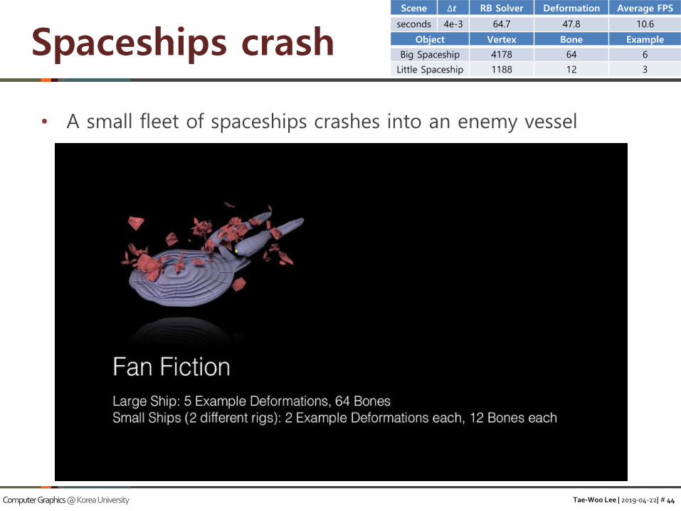
Spaceships crash Object Vertex Bone Example
Big Spaceship 4178 64 6
Little Spaceship 1188 12 3
Scene ∆𝒕 RB Solver Deformation Average FPS
seconds 4e-3 64.7 47.8 10.6
• A small fleet of spaceships crashes into an enemy vessel
Tae-Woo Lee | 2019-04-22| # 45Computer Graphics @ Korea University
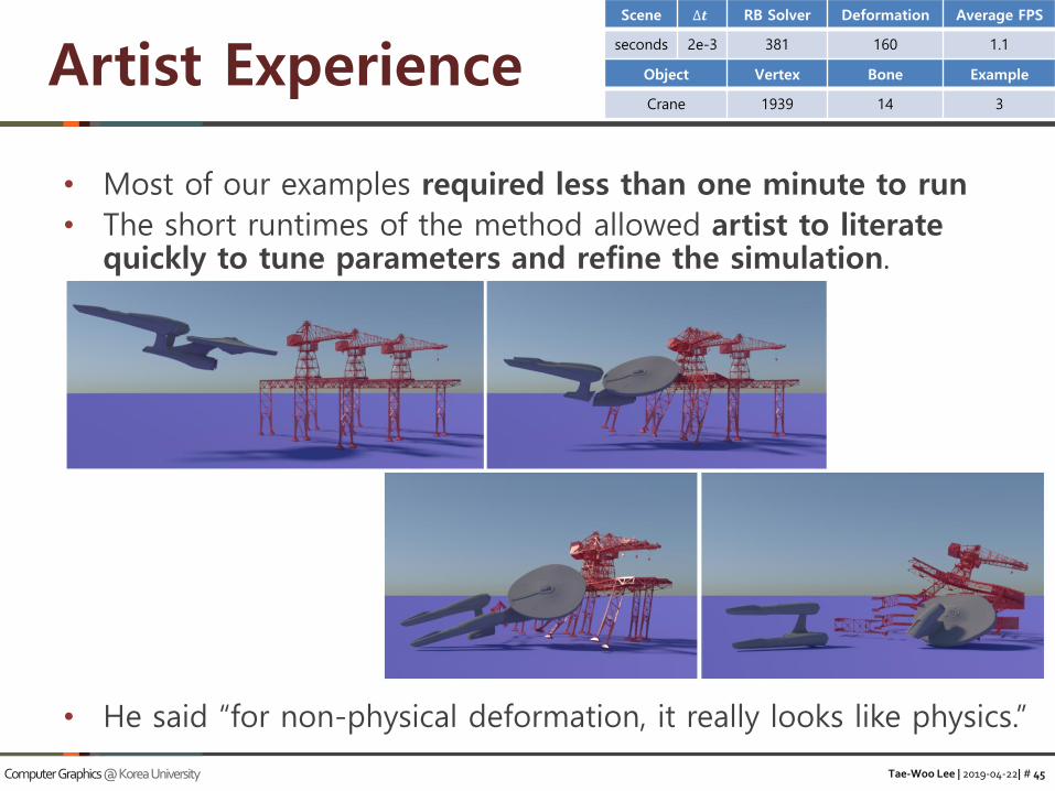
• Most of our examples required less than one minute to run
• The short runtimes of the method allowed artist to literatequickly to tune parameters and refine the simulation.
• He said “for non-physical deformation, it really looks like physics.”
Artist Experience Object Vertex Bone Example
Crane 1939 14 3
Scene ∆𝒕 RB Solver Deformation Average FPS
seconds 2e-3 381 160 1.1
Tae-Woo Lee | 2019-04-22| # 46Computer Graphics @ Korea University
Performance
• Depending on the scene,out method adds 42% to 59% overhead per timestep on average(excluding the scene of spaceships crash)
• Several of our examples run in real-time, while the rest are fastenough to allow artists to interactively tune parameters
• The examples in this paper were run on a 2013 Macbook Prowith an integrated GPU
• The projection and propagation were parallelized on the CPUwhile skinning was performed on the GPU

Tae-Woo Lee | 2019-04-22| # 47Computer Graphics @ Korea University
Summary
• Our method targets extreme destructive scenes
• The underlying examples have a complex relationshipwith the final animation
• A technique for animating the failure of near-rigidman-made materials
• Fast, artist friendly, easily implemented,integrates smoothly into existing pipeline!

Tae-Woo Lee | 2019-04-22| # 48Computer Graphics @ Korea University
Limitations and Future Work
• Automatically generated rig was only able to approximatethe shapes in the simulation output.⟶ Improved automatic rig generation
• Examples deliberately use a small number of example deformation
⟶ Reducing the burden on the artist
• Smoothness of the example weights or favoring using a single example over an average of all examples
⟶ Computing the example weights