Examining Your Data

LEARNING OBJECTIVES

Upon completing this chapter, you should be able to do the following:

• Select the appropriate graphical method to examine the characteristics of the data or relationships of interest.

• Assess the type and potential impact of missing data.

• Understand the different types of missing data processes.

• Explain the advantages and disadvantages of the approaches available for dealing with missing data.

• Identify univariate, bivariate, and multivariate outliers.

• Test your data for the assumptions underlying most multivariate techniques.

• Determine the best method of data transformation given a specific problem.

• Understand how to incmporate nonmetric variables as metric variables.

CHAPTER PREVIEW

Data examination is a time-consuming, but necessary, initial step in any analysis that researchers often overlook. Here the researcher evaluates the impact of missing data, identifies outliers, and tests for the assumptions underlying most multivariate techniques. The objective of these data examination tasks is as much to reveal what is not apparent as it is to portray the actual data, because the "hidden" effects are easily overlooked. For example, the biases introduced by nonran­dom missing data will never be known unless explicitly identified and remedied by the methods dis­cussed in a later section of this chapter. Moreover, unless the researcher reviews the results on a case-by-case basis, the existence of outliers will not be apparent, even if they substantially affect the results. Violations of the statistical assumption may cause biases or nonsignificance in the results that cannot be distinguished from the true results.

Before we discuss a series of empirical tools to aid in data examination, the introductory section of this chapter offers a summary of various graphical techniques available to the researcher as a means of representing data. These techniques provide the researcher with a set of simple yet comprehensive ways to examine both the individual variables and the relationships among them. The graphical techniques are not meant to replace the empirical tools, but rather provide a comple­mentary means of portraying the data and its relationships. As you will see, a histogram can graph­ically show the shape of a data distribution, just as we can reflect that same distribution with

From Chapter 2 of Multivariate Data Analysis, 7/e. Joseph F. Hair, Jr .• William C. Black. Barry J. Babin, Rolph E. Anderson. Copyright 0 2010 by Pearson Prentice Hall. All rights reserved.

Examining Your Data

skewness and kurtosis values. The empirical measures quantify the distribution's characteristics, whereas the histogram portrays them in a simple and visual manner. Likewise, other graphical tech­niques (i.e., scatterplot and boxplot) show relationships between variables represented by the corre­lation coefficient and means difference test, respectively.

With the graphical techniques addressed, the next task facing the researcher is how to assess and overcome pitfalls resulting from the research design (e.g., questionnaire design) and data col­lection practices. Specifically, this chapter addresses the following:

• Evaluation of missing data • Identification of outliers • Testing of the assumptions underlying most multivariate techniques

Missing data are a nuisance to researchers and primarily result from errors in data collection or data entry or from the omission of answers by respondents. Classifying missing data and the rea­sons underlying their presence are addressed through a series of steps that not only identify the impacts of the missing data, but that also provide remedies for dealing with it in the analysis. Outliers, or extreme responses, may unduly influence the outcome of any multivariate analysis. For this reason, methods to assess their impact are discussed. Finally, the statistical assumptions underlying most multivariate analyses are reviewed. Before applying any multivariate technique, the researcher must assess the fit of the sample data with the statistical assumptions underlying that multivariate technique. For example, researchers wishing to apply regression analysis would be par­ticularly interested in assessing the assumptions of normality, homoscedasticity, independence of error, and linearity. Each of these issues should be addressed to some extent for each application of a multivariate technique.

In addition, this chapter introduces the researcher to methods of incorporating nonmetric variables in applications that require metric variables through the creation of a special type of metric variable known as dummy variables. The applicability of using dummy variables varies with each data analysis project.

KEY TERMS

Before starting the chapter, review the key terms to develop an understanding of the concepts and ter­minology used. Throughout the chapter the key terms appear in boldface. Other points of emphasis in the chapter and key term cross-references are italicized.

AU-available approach Imputation method for missing data that computes values based on all-available valid observations, also known as the pairwise approach.

Boxplot Method of representing the distribution of a variable. A box represents the major portion of the distribution, and the extensions-called whiskers-reach to the extreme points of the dis­tribution. This method is useful in making comparisons of one or more variables across groups.

Censored data Observations that are incomplete in a systematic and known way. One example occurs in the study of causes of death in a sample in which some individuals are still living. Censored data are an example of ignorable missing data.

Comparison group See reference category. Complete case approach Approach for handling missing data that computes values based on

data from complete cases, that is, cases with no missing data. Also known as the listwise approach.

Data transformations A variable may have an undesirable characteristic, such as nonnormality, that detracts from its use in a multivariate technique. A transformation, such as taking the logarithm or square root of the variable, creates a transformed variable that is more suited to portraying the relationship. Transformations may be applied to either the dependent or independent variables, or

Examining Your Data

both. The need and specific type of transformation may be based on theoretical reasons (e.g., trans­forming a known nonlinear relationship) or empirical reasons (e.g., problems identified through graphical or statistical means).

Dummy variable Special metric variable used to represent a single category of a nonmetric variable. To account for L levels of a nonmetric variable, L - 1 dummy variables are needed. For example, gender is measured as male or female and could be represented by two dummy variables (X1 and X2). When the respondent is male, X1 = 1 and X2 = 0. Likewise, when the respondent is female, X1 = 0 and X2 = 1. However, when X1 = 1, we know that X2 must equal 0. Thus, we need only one variable, either X1 or X2, to represent the variable gender. H a nonmetric variable has three levels, only two dummy variables are needed. We always have one dummy variable less than the number of levels for the nonmetric variable. The omitted category is termed the reference category.

Effects coding Method for specifying the reference category for a set of dummy variables where the reference category receives a value of minus one ( -1) across the set of dummy variables. With this type of coding, the dummy variable coefficients represent group deviations from the mean of all groups, which is in contrast to indicator coding.

Heteroscedasticity See homoscedasticity. Histogram Graphical display of the distribution of a single variable. By forming frequency

counts in categories, the shape of the variable's distribution can be shown. Used to make a visual comparison to the normal distribution.

Homoscedasticity When the variance of the error terms (e) appears constant over a range of predictor variables, the data are said to be homoscedastic. The assumption of equal variance of the population errorE (where E is estimated from e) is critical to the proper application of many multivariate techniques. When the error terms have increasing or modulating variance, the data are said to be heteroscedastic. Analysis of residuals best illustrates this point

Ignorable missing data Missing data process that is explicitly identifiable and/or is under the control of the researcher. Ignorable missing data do not require a remedy because the missing data are explicitly handled in the technique used.

Imputation Process of estimating the missing data of an observation based on valid values of the other variables. The objective is to employ known relationships that can be identified in the valid values of the sample to assist in representing or even estimating the replacements for missing values.

Indicator coding Method for specifying the reference category for a set of dummy variables where the reference category receives a value of zero across the set of dummy variables. The dummy variable coefficients represent the category differences from the reference category. Also see effects coding.

Kurtosis Measure of the peakedness or flatness of a distribution when compared with a normal distribution. A positive value indicates a relatively peaked distribution, and a negative value indi­cates a relatively flat distribution.

Linearity Used to express the concept that the model possesses the properties of additivity and homogeneity. In a simple sense, linear models predict values that fall in a straight line by having a constant unit change (slope) of the dependent variable for a constant unit change of the inde­pendent variable. In the population model Y = b0 + b1X1 + e, the effect of a change of 1 in X1 is to add b1 (a constant) units to Y.

Missing at random (MAR) Classification of missing data applicable when missing values of Y depend on X, but not on Y. When missing data are MAR, observed data for Yare a truly random sample for the X values in the sample, but not a random sample of all Y values due to missing values of X.

Missing completely at random (MCAR) Classification of missing data applicable when missing values of Yare not dependent on X. When missing data are MCAR, observed values of Y are a truly random sample of all Y values, with no underlying process that lends bias to the observed data.

Examining Your Data

Missing data Information not available for a subject (or case) about whom other information is available. Missing data often occur when a respondent fails to answer one or more questions in a survey.

Missing data process Any systematic event external to the respondent (such as data entry errors or data collection problems) or any action on the part of the respondent (such as refusal to answer a question) that leads to missing data.

Multivariate graphical display Method of presenting a multivariate profile of an observation on three or more variables. The methods include approaches such as glyphs, mathematical transfor­mations, and even iconic representations (e.g., faces).

Normal distribution Purely theoretical continuous probability distribution in which the horiwn­tal axis represents all possible values of a variable and the vertical axis represents the probability of those values occurring. The scores on the variable are clustered around the mean in a symmet­rical, unimodal pattern known as the bell-shaped, or normal, curve.

Normal probability plot Graphical comparison of the form of the distribution to the normill distri­butioTL In the normal probability plot. the normal distribution is represented by a straight line angled at 45 degrees. The actual distribution is plotted against this line so that any differences are shown as devi­ations fium the straight line, making identification of differences quite apparent and interpretable.

Normality Degree to which the distribution of the sample data corresponds to a normill distributioTL Outlier An observation that is substantially different fium the other observations (i.e., has an extreme

value) on one or more characteristics (variables). At issue is its representativeness of the population. Reference category The category of a nonmetric variable that is omitted when creating dummy

variables and acts as a reference point in interpreting the dummy variables. In indicator coding, the reference category has values of zero (0) for all dummy variables. With effects coding, the ref­erence category has values of minus one (-1) for all dummy variables.

Residual Portion of a dependent variable not explained by a multivariate technique. Associated with dependence methods that attempt to predict the dependent variable, the residual represents the unexplained portion of the dependent variable. Residuals can be used in diagnostic procedures to identify problems in the estimation technique or to identify unspecified relationships.

Robustness The ability of a statistical technique to perform reasonably well even when the underlying statistical assumptions have been violated in some manner.

Scatterplot Representation of the relationship between two metric variables portraying the joint values of each observation in a two-dimensional graph.

Skewness Measure of the symmetry of a distribution; in most instances the comparison is made to a normal distributioTL A positively skewed distribution has relatively few large values and tails off to the right. and a negatively skewed distribution has relatively few small values and tails off to the left. Skewness values falling outside the range of -1 to + 1 indicate a substantially skewed distribution.

Variate Linear combination of variables formed in the multivariate technique by deriving empir­ical weights applied to a set of variables specified by the researcher.

INTRODUCTION

The tasks involved in examining your data may seem mundane and inconsequential, but they are an essential part of any multivariate analysis. Multivariate techniques place tremendous analytical power in the researcher's hands. But they also place a greater burden on the researcher to ensure that the statistical and theoretical underpinnings on which they are based also are supported. By examin­ing the data before the application of any multivariate technique, the researcher gains several criti­cal insights into the characteristics of the data:

• First and foremost. the researcher attains a basic understanding of the data and relationships between variables. Multivariate techniques place greater demands on the researcher to under­stand, interpret. and articulate results based on relationships that are more complex than

Examining Your Data

encountered before. A thorough knowledge of the variable interrelationships can aid immea­surably in the specification and refinement of the multivariate model as well as provide a reasoned perspective for interpretation of the results.

• Second, the researcher ensures that the data underlying the analysis meet all of the require­ments for a multivariate analysis. Multivariate techniques demand much more from the data in terms of larger data sets and more complex assumptions than encountered with univariate analyses. Missing data, outliers, and the statistical characteristics of the data are all much more difficult to assess in a multivariate context. Thus, the analytical sophistica­tion needed to ensure that these requirements are met forces the researcher to use a series of data examination techniques that are as complex as the multivariate techniques themselves.

Both novice and experienced researchers may be tempted to skim or even skip this chapter to spend more time in gaining knowledge of a multivariate technique(s). The time, effort, and resources devoted to the data examination process may seem almost wasted because many times no corrective action is warranted. The researcher should instead view these techniques as "investments in multi­variate insurance" that ensure the results obtained from the multivariate analysis are truly valid and accurate. Without such an ''investment" it is quite easy, for example, for several unidentified outliers to skew the results, for missing data to introduce a bias in the correlations between variables, or for nonnormal variables to invalidate the results. And yet the most troubling aspect of these problems is that they are "hidden;' because in most instances the multivariate techniques will go ahead and pro­vide results. Only if the researcher has made the ''investment" will the potential for catastrophic problems be recognized and corrected before the analyses are performed. These problems can be avoided by following these analyses each and every time a multivariate technique is applied. These efforts will more than pay for themselves in the long run; the occurrence of one serious and possi­bly fatal problem will make a convert of any researcher. We encourage you to embrace these tech­niques before problems that arise during analysis force you to do so.

GRAPHICAL EXAMINATION OF THE DATA

As discussed earlier, the use of multivariate techniques places an increased burden on the researcher to understand, evaluate, and interpret complex results. This complexity requires a thorough under­standing of the basic characteristics of the underlying data and relationships. When univariate analyses are considered, the level of understanding is fairly simple. As the researcher moves to more complex multivariate analyses, however, the need and level of understanding increase dramatically and require even more powerful empirical diagnostic measures. The researcher can be aided immea­surably in gaining a fuller understanding of what these diagnostic measures mean through the use of graphical techniques, portraying the basic characteristics of individual variables and relationships between variables in a simple "picture." For example, a simple scatterplot represents in a single pic­ture not only the two basic elements of a correlation coefficient, namely the type of relationship (positive or negative) and the strength of the relationship (the dispersion of the cases), but also a simple visual means for assessing linearity that would require a much more detailed analysis if attempted strictly by empirical means. Correspondingly, a boxplot illustrates not only the overall level of differences across groups shown in a t-test or analysis of variance, but also the differences between pairs of groups and the existence of outliers that would otherwise take more empirical analysis to detect if the graphical method was not employed. The objective in using graphical tech­niques is not to replace the empirical measures, but to use them as a complement to provide a visual representation of the basic relationships so that researchers can feel confident in their understanding of these relationships.

The advent and widespread use of statistical programs designed for the personal computer increased access to such methods. Most statistical programs provide comprehensive modules of

Examining Your Data

graphical techniques available for data examination that are augmented with more detailed statistical measures of data description. The following sections detail some of the more widely used techniques for examining the characteristics of the distribution, bivariate relationships, group differences, and even multivariate profiles.

Univariate Profiling: Examining the Shape of the Distribution

The starting point for understanding the nature of any variable is to characterize the shape of its distribution. A number of statistical measures are discussed in a later section on normality, but many times the researcher can gain an adequate perspective of the variable through a histogram. A histogram is a graphical representation of a single variable that represents the frequency of occur­rences (data values) within data categories. The frequencies are plotted to examine the shape of the distribution of values. H the integer values ranged from 1 to 10, the researcher could construct a histogram by counting the number of responses for each integer value. For continuous variables, categories are formed within which the frequency of data values is tabulated. H examination of the distribution is to assess its normality (see section on testing assumptions for details on this issue), the normal curve can be superimposed on the distribution to assess the correspondence of the actual distribution to the desired (normal) distribution. The histogram can be used to examine any type of metric variable.

For example, the responses for X6 from the HBAT database are represented in Figure 1. The height of the bars represents the frequencies of data values within each category. The normal curve is also superimposed on the distribution. As will be shown in a later section, empirical measures indicate that the distribution of A{; deviates significantly from the normal distribution. But how does it differ? The empirical measure that differs most is the kurtosis, representing the peakedness or flat­ness of the distribution. The values indicate that the distribution is flatter than expected. What does the histogram show? The middle of the distribution falls below the superimposed normal curve, while both tails are higher than expected. Thus, the distribution shows no appreciable skewness to one side or the other, just a shortage of observations in the center of the distribution. This compari­son also provides guidance on the type of transformation that would be effective if applied as a rem­edy for nonnormality. All of this information about the distribution is shown through a single histogram.

15

§ 10 0 u

5

6.0 7.0 8.0 9.0

Xt; Product Quality

Examining Your Data

Bivariate Profiling: Examining the Relationship Between Variables

Whereas examining the distribution of a variable is essential, many times the researcher is also interested in examining relationships between two or more variables. The most popular method for examining bivariate relationships is the scatterplot, a graph of data points based on two metric vari­ables. One variable defines the horizontal axis and the other variable defines the vertical axis. Variables may be any metric value. The points in the graph represent the corresponding joint values of the variables for any given case. The pattern of points represents the relationship between the variables. A strong organization of points along a straight line characterizes a linear relationship or correlation. A curved set of points may denote a nonlinear relationship, which can be accommo­dated in many ways (see later discussion on linearity). Or a seemingly random pattern of points may indicate no relationship.

Of the many types of scatterplots, one format particularly suited to multivariate techniques is the scatterplot matrix, in which the scatterplots are represented for all combinations of variables in the lower portion of the matrix. The diagonal contains histograms of the variables. Scatterplot matrices and individual scatterplots are now available in all popular statistical programs. A variant of the scatterplot is discussed in the following section on outlier detection, where an ellipse representing a specified confidence interval for the bivariate normal distribution is superimposed to allow for outlier identification.

Figure 2 presents the scatterplots for a set of five variables from the HBAT database (A{;, X7,

Xs, X12, and Xn). For example, the highest correlation can be easily identified as between X7 and X12,

Note: Values above the diagonal are bivariate mrrelations, with corresponding scatterplot below the diagonal. Diagonal portrays the distribution of each variable.

Examining Your Data

as indicated by the observations closely aligned in a well-defined linear pattern. In the opposite extreme, the correlation just above (X7 versus X8) shows an almost total lack of relationship as evidenced by the widely dispersed pattern of points and the correlation .001. Finally, an inverse or negative relationship is seen for several combinations, most notably the correlation of A{; and X13

(- .401). Moreover, no combination seems to exhibit a nonlinear relationship that would not be represented in a bivariate correlation.

The scatterplot matrix provides a quick and simple method of not only assessing the strength and magnitude of any bivariate relationship, but also a means of identifying any nonlinear patterns that might be hidden if only the bivariate correlations, which are based on a linear relationship, are examined.

Bivariate Profiling: Examining Group Differences

The researcher also is faced with understanding the extent and character of differences of one or more metric variables across two or more groups formed from the categories of a nonmetric vari­able. Assessing group differences is done through univariate analyses such as t-tests and analysis of variance and the multivariate techniques of discriminant analysis and multivariate analysis of vari­ance. Another important aspect is to identify outliers (described in more detail in a later section) that may become apparent only when the data values are separated into groups.

The graphical method used for this task is the boxplot, a pictorial representation of the data distribution of a metric variable for each group (category) of a nonmetric variable (see example in Figure 3). First, the upper and lower quartiles of the data distribution form the upper and lower boundaries of the box, with the box length being the distance between the 25th percentile and the 75th percentile. The box contains the middle 50 percent of the data values and the larger the box, the greater the spread (e.g., standard deviation) of the observations. The median is depicted by a solid line within the box. H the median lies near one end of the box, skewness in the opposite direction is indicated. The lines extending from each box (called whiskers) represent the distance to the small­est and the largest observations that are less than one quartile range from the box. Outliers (observa­tions that range between 1.0 and 1.5 quartiles away from the box) and extreme values (observations greater than 1.5 quartiles away from the end of the box) are depicted by symbols outside the whiskers. In using boxplots, the objective is to portray not only the information that is given in the

6

n.-----------------------------, 013 090

OSJ

022

10

013

5

4~----L-------~--------~----~

Less than 1year

1 to 5 years More than 5years

X1 Customer Type

2

Less than 1year

1 to5years

X1 Customer Type

Over 5years

Examining Your Data

statistical tests (Are the groups different?), but also additional descriptive information that adds to our understanding of the group differences.

Figure 3 shows the boxplots for X6 and X7 for each of the three groups of X1 (Customer Type). Before examining the boxplots for each variable, let us first see what the statistical tests tell us about the differences across these groups for each variable. For A{;, a simple analysis of variance test indicates a highly significant statistical difference (F value of 36.6 and a significance level of .000) across the three groups. For X7, however, the analysis of variance test shows no statistically significant difference (significance level of .419) across the groups of X1.

Using boxplots, what can we learn about these same group differences? As we view the boxplot of X6, we do see substantial differences across the groups that confirm the statistical results. We can also see that the primary differences are between groups 1 and 2 versus group 3. Essentially, groups 1 and 2 seem about equal. If we performed more statistical tests looking at each pair of groups separately, the tests would confirm that the only statistically significant differ­ences are group 1 versus 3 and group 2 versus 3. Also, we can see that group 2 has substantially more dispersion (a larger box section in the boxplot), which prevents its difference from group 1. The boxplots thus provide more information about the extent of the group differences of X6 than just the statistical test.

For X7, we can see that the three groups are essentially equal. as verified by the nonsignificant statistical test. We can also see a number of outliers in each of the three groups (as indicated by the notations at the upper portion of each plot beyond the whiskers). Although the outliers do not impact the group differences in this case, the researcher is alerted to their presence by the boxplots. The researcher could examine these observations and consider the possible remedies discussed in more detail later in this chapter.

Multivariate Profiles

To this point the graphical methods have been restricted to univariate or bivariate portrayals. In many instances, however, the researcher may desire to compare observations characterized on a multivariate profile, whether it be for descriptive purposes or as a complement to analytical procedures. To address this need, a number of multivariate graphical displays center around one of three types of graphs [10]. The first graph type is a direct portrayal of the data values, either by (a) glyphs, or metroglyphs, which are some form of circle with radii that correspond to a data value; or (b) multivariate profiles, which portray a bar like profile for each observation. A second type of multivariate display involves a mathematical transformation of the original data into a mathematical relationship, which can then be portrayed graphically. The most com­mon technique of this type is Andrew's Fourier transformation [1 ]. The final approach is the use of graphical displays with iconic representativeness, the most popular being a face [5]. The value of this type of display is the inherent processing capacity humans have for their interpre­tation. As noted by Chernoff [5]:

I believe that we learn very early to study and react to real faces. Our library of responses to faces exhausts a large part of our dictionary of emotions and ideas. We perceive the faces as a gestalt and our built-in computer is quick to pick out the rele­vant information and to filter out the noise when looking at a limited number of faces.

Facial representations provide a potent graphical format but also give rise to a number of con­siderations that affect the assignment of variables to facial features, unintended perceptions, and the quantity of information that can actually be accommodated. Discussion of these issues is beyond the scope of this chapter, and interested readers are encouraged to review them before attempting to use these methods [24, 25].

Examining Your Data

The researcher can employ any of these methods when examining multivariate data to provide a format that is many times more insightful than just a review of the actual data values. Moreover, the multivariate methods enable the researcher to use a single graphical portrayal to represent a large number of variables, instead of using a large number of the univariate or bivariate methods to portray the same number of variables.

MISSING DATA

Missing data, where valid values on one or more variables are not available for analysis, are a fact of life in multivariate analysis. In fact, rarely does the researcher avoid some form of missing data problem. The researcher's challenge is to address the issues raised by missing data that affect the generalizability of the results. To do so, the researcher's primary concern is to identify the patterns and relationships underlying the missing data in order to maintain as close as possible the original distribution of values when any remedy is applied. The extent of missing data is a secondary issue in most instances, affecting the type of remedy applied. These patterns and relationships are a result of a missing data process, which is any systematic event external to the respondent (such as data entry errors or data collection problems) or any action on the part of the respondent (such as refusal to answer) that leads to missing values. The need to focus on the reasons for missing data comes from the fact that the researcher must understand the processes leading to the missing data in order to select the appropriate course of action.

The lmpad of Missing Data

The effects of some missing data processes are known and directly accommodated in the research plan as will be discussed later in this section. More often, the missing data processes, particularly those based on actions by the respondent (e.g., nonresponse to a question or set of questions), are rarely known beforehand. To identify any patterns in the missing data that would characterize the missing data process, the researcher asks such questions as (1) Are the missing data scattered randomly throughout the observations or are distinct patterns identifi­able? and (2) How prevalent are the missing data? If distinct patterns are found and the extent of missing data is sufficient to warrant action, then it is assumed that some missing data process is in operation.

Why worry about the missing data processes? Can't the analysis be performed with the valid values we do have? Although it might seem prudent to proceed just with the valid values, both substantive and practical considerations necessitate an examination of the missing data processes.

• The practical impact of missing data is the reduction of the sample size available for analysis. For example, if remedies for missing data are not applied, any observation with missing data on any of the variables will be excluded from the analysis. In many multivariate analyses, par­ticularly survey research applications, missing data may eliminate so many observations that what was an adequate sample is reduced to an inadequate sample. For example, it has been shown that if 10 percent of the data is randomly missing in a set of five variables, on average almost 60 percent of the cases will have at least one missing value [17]. Thus, when complete data are required, the sample is reduced to 40 percent of the original size. In such situations, the researcher must either gather additional observations or find a remedy for the missing data in the original sample.

• From a substantive perspective, any statistical results based on data with a nonrandom miss­ing data process could be biased. This bias occurs when the missing data process "causes" certain data to be missing and these missing data lead to erroneous results. For example, what if we found that individuals who did not provide their household income tended to be almost exclusively those in the higher income brackets? Wouldn't you be suspect of the results

Examining Your Data

knowing this specific group of people were excluded? The effects of missing data are some­times termed hidden due to the fact that we still get results from the analyses even without the missing data. The researcher could consider these biased results as valid unless the underlying missing data processes are identified and understood.

The concern for missing data processes is similar to the need to understand the causes of nonresponse in the data collection process. Just as we are concerned about who did not respond during data collection and any subsequent biases, we must also be concerned about the nonresponse or miss­ing data among the collected data. The researcher thus needs to not only remedy the missing data if possible, but also understand any underlying missing data processes and their impacts. Yet, too often, researchers either ignore the missing data or invoke a remedy without regard to the effects of the miss­ing data. The next section employs a simple example to illustrate some of these effects and some simple, yet effective, remedies. Then, a four-step process of identifying and remedying missing data processes is presented. Finally, the four-step process is applied to a small data set with missing data.

A Simple Example of a Missing Data Analysis

To illustrate the substantive and practical impacts of missing data, Table 1 contains a simple example of missing data among 20 cases. As is typical of many data sets, particularly in survey research, the number of missing data varies widely among both cases and variables.

In this example, we can see that all of the variables (V1 to Vs) have some missing data, with V3 missing more than one-half (55%) of all values. Three cases (3, 13, and 15) have more

TABLE1 Hypothetical Example of Missing Data

Missing Data by Case

CaseiD v, v2 v3 v4 Vs Number Percent

1 1.3 9.9 6.7 3.0 2.6 0 0 2 4.1 5.7 2.9 2 40 3 9.9 3.0 3 60 4 .9 8.6 2.1 1.8 20 5 .4 8.3 1.2 1.7 20 6 1.5 6.7 4.8 2.5 20 7 .2 8.8 4.5 3.0 2.4 0 0 8 2.1 8.0 3.0 3.8 1.4 0 0 9 1.8 7.6 3.2 2.5 20

10 4.5 8.0 3.3 2.2 20 11 2.5 9.2 3.3 3.9 20 12 4.5 6.4 5.3 3.0 2.5 0 9 13 2.7 4 80 14 2.8 6.1 6.4 3.8 1 20 15 3.7 3.0 3 60 16 1.6 6.4 5.0 2.1 20 17 .5 9.2 3.3 2.8 20 18 2.8 5.2 5.0 2.7 20 19 2.2 6.7 2.6 2.9 20 20 1.8 9.0 5.0 2.2 3.0 0 0

Missing Data by Variable Total Missing Values Number 2 2 11 6 2 Number: 23 Percent 10 10 55 30 10 Percent: 23

Examining Your Data

than 50 percent missing data and only five cases have complete data. Overall, 23 percent of the data values are missing.

From a practical standpoint, the missing data in this example can become quite problematic in terms of reducing the sample size. For example, if a multivariate analysis was performed that required complete data on all five variables, the sample would be reduced to only the five cases with no missing data (cases 1, 7, 8, 12, and 20). This sample size is too few for any type of analysis. Among the remedies for missing data that will be discussed in detail in later sections, an obvious option is the elimination of variables and/or cases. In our example, assuming that the conceptual foundations of the research are not altered substantially by the deletion of a variable, eliminating V3

is one approach to reducing the number of missing data. By just eliminating V3, seven additional cases, for a total of 12, now have complete information. H the three cases (3, 13, 15) with exception­ally high numbers of missing data are also eliminated, the total number of missing data is now reduced to only five instances, or 7.4 percent of all values.

The substantive impact, however, can be seen in these five that are still missing data; all occur in V4. By comparing the values of V2 for the remaining five cases with missing data for V4 (cases 2, 6, 14, 16, and 18) versus those cases having valid V4 values, a distinct pattern emerges. The five cases with missing values for V4 have the five lowest values for V2, indicating that miss­ing data for V4 are strongly associated with lower scores on V2. This systematic association between missing and valid data directly affects any analysis in which V4 and V2 are both included. For example, the mean score for V2 will he higher if cases with missing data on V4 are excluded (mean= 8.4) than if those five cases are included (mean= 7.8). In this instance, the researcher must always scrutinize results including both v4 and v2 for the possible impact of this missing data process on the results.

As we have seen in the example, finding a remedy for missing data (e.g., deleting cases or variables) can be a practical solution for missing data. Yet the researcher must guard against apply­ing such remedies without diagnosis of the missing data processes. Avoiding the diagnosis may address the practical problem of sample size, but only cover up the substantive concerns. What is needed is a structured process of first identifying the presence of missing data processes and then applying the appropriate remedies. In the next section we discuss a four-step process to address both the practical and substantive issues arising from missing data.

A Four-Step Process for Identifying Missing Data and Applying Remedies

As seen in the previous discussions, missing data can have significant impacts on any analysis, par­ticularly those of a multivariate nature. Moreover, as the relationships under investigation become more complex, the possibility also increases of not detecting missing data processes and their effects. These factors combine to make it essential that any multivariate analysis begin with an examination of the missing data processes. To this end, a four-step process (see Figure 4) is pre­sented, which addresses the types and extent of missing data, identification of missing data processes, and available remedies for accommodating missing data into multivariate analyses.

STEP 1: DETERMINE THE TYPE OF MISSING DATA The first step in any examination of missing data is to determine the type of missing data involved. Here the researcher is concerned whether the missing data are part of the research design and under the control of the researcher or whether the "causes" and impacts are truly unknown. Let's start with the missing data that are part of the research design and can be handled directly by the researcher.

Ignorable Missing Data. Many times, missing data are expected and part of the research design. In these instances, the missing data are termed ignorable missing data, meaning that specific remedies for missing data are not needed because the allowances for missing data are inherent in the technique used [18, 22]. The justification for designating missing data as ignorable is that the miss­ing data process is operating at random (i.e., the observed values are a random sample of the total set

Examining Your Data

Step 1: Determine the Type of Missing Data

Apply specialized Yi techniques for

es - ignorable missing data

MAR

Is the missing data ignorable?

Delete cases and/or variables

with high missing data

No

Yes

No

Step 4: Select the Imputation Method

Do you want to replace the missing data with values?

Select the Data Application Method

Do you want to use only cases with complete data or use all

possible valid data?

Select the Data Application Method

Do you want to use known values or calculate replacement values

from the valid data?

Complete Data Only 1 Possible Data r Known Values

---L._--... Modeling­

Based Approaches

l Complete

Case Approach

All­Available­

Subsets Approach

Case Substitution

Hot and Cold Deck Imputation

Mean Substitution

FIGURE 4 A Four-Step Process for Identifying Missing Data and Applying Remedies

Regression­Based

Approach

Examining Your Data

of values, observed and missing) or explicitly accommodated in the technique used. There are three instances in which a researcher most often encounters ignorable missing data.

• The first example encountered in almost all surveys and most other data sets is the ignorable missing data process resulting from taking a sample of the population rather than gathering data from the entire population. In these instances, the missing data are those observations in a population that are not included when taking a sample. The purpose of multivariate tech­niques is to generalize from the sample observations to the entire population, which is really an attempt to overcome the missing data of observations not in the sample. The researcher makes these missing data ignorable by using probability sampling to select respondents. Probability sampling enables the researcher to specify that the missing data process leading to the omitted observations is random and that the missing data can be accounted for as sampling error in the statistical procedures. Thus, the missing data of the nonsampled observations are ignorable.

• A second instance of ignorable missing data is due to the specific design of the data collection process. Certain nonprobability sampling plans are designed for specific types of analysis that accommodate the nonrandom nature of the sample. Much more common are missing data due to the design of the data collection instrument, such as through skip patterns where respon­dents skip sections of questions that are not applicable.

For example, in examining customer complaint resolution, it might be appropriate to require that individuals make a complaint before asking questions about how complaints are handled. For those respondents not making a complaint, they do not answer the ques­tions on the process and thus create missing data. The researcher is not concerned about these missing data, because they are part of the research design and would be inappropriate to attempt to remedy.

• A third type of ignorable missing data occurs when the data are censored. Censored data are observations not complete because of their stage in the missing data process. A typical example is an analysis of the causes of death. Respondents who are still living cannot pro­vide complete information (i.e., cause or time of death) and are thus censored. Another inter­esting example of censored data is found in the attempt to estimate the heights of the U.S. general population based on the heights of armed services recruits (as cited in [18]). The data are censored because in certain years the armed services had height restrictions that varied in level and enforcement. Thus, the researchers face the task of estimating the heights of the entire population when it is known that certain individuals (i.e., all those below the height restrictions) are not included in the sample. In both instances the researcher's knowledge of the missing data process allows for the use of specialized methods, such as event history analysis, to accommodate censored data [18].

In each instance of an ignorable missing data process, the researcher has an explicit means of accommodating the missing data into the analysis. It should be noted that it is possible to have both ignorable and nonignorable missing data in the same data set when two different missing data processes are in effect.

Missing Data Processes That Are Not Ignorable. Missing data that cannot be classified as ignorable occur for many reasons and in many situations. In general, these missing data fall into two classes based on their source: known versus unknown processes.

• Many missing data processes are known to the researcher in that they can be identified due to procedural factors, such as errors in data entry that create invalid codes, disclosure restrictions (e.g., small counts in U.S. Census data), failure to complete the entire questionnaire, or even the morbidity of the respondent. In these situations, the researcher has little control over the missing data processes, but some remedies may be applicable if the missing data are found to be random.

Examining Your Data

• Unknown missing data processes are less easily identified and accommodated. Most often these instances are related directly to the respondent. One example is the refusal to respond to certain questions, which is common in questions of a sensitive nature (e.g., income or controversial issues) or when the respondent has no opinion or insufficient knowledge to answer the question. The researcher should anticipate these problems and attempt to mini­mize them in the research design and data collection stages of the research. However, they still may occur, and the researcher must now deal with the resulting missing data. But all is not lost. When the missing data occur in a random pattern, remedies may be available to mitigate their effect.

In most instances, the researcher faces a missing data process that cannot be classified as ignornble. Whether the source of this nonignorable missing data process is known or unknown, the researcher must still proceed to the next step of the process and assess the extent and impact of the missing data.

STEP 2: DETERMINE THE EXTENT OF MISSING DATA Given that some of the missing data are not ignorable, the researcher must next examine the patterns of the missing data and determine the extent of the missing data for individual variables, individual cases, and even overall. The primary issue in this step of the process is to determine whether the extent or amount of missing data is low enough to not affect the results, even if it operates in a nonrandom manner. H it is sufficiently low, then any of the approaches for remedying missing data may be applied. H the missing data level is not low enough, then we must first determine the randomness of the missing data process before selecting a remedy (step 3). The unresolved issue at this step is this question: What is low enough? In making the assessment as to the extent of missing data, the researcher may find that the deletion of cases and/or variables will reduce the missing data to levels that are low enough to allow for remedies without concern for creating biases in the results.

Assessing the Extent and Patterns of Missing Data. The most direct means of assessing the extent of missing data is by tabulating ( 1) the percentage of variables with missing data for each case and (2) the number of cases with missing data for each variable. This simple process identifies not only the extent of missing data, but any exceptionally high levels of missing data that occur for individual cases or observations. The researcher should look for any nonrandom patterns in the data, such as concentration of missing data in a specific set of questions, attrition in not completing the questionnaire, and so on. Finally, the researcher should determine the number of cases with no missing data on any of the variables, which will provide the sample size available for analysis if remedies are not applied.

With this information in hand, the important question is: Is the missing data so high as to warrant additional diagnosis? At issue is the possibility that either ignoring the missing data or using some remedy for substituting values for the missing data can create a bias in the data that will markedly affect the results. Even though most discussions of this issue require researcher judgment, the two guidelines in Rules of Thumb 1 apply.

RULES OF THUMB 1

How Much Missing Data Is Too Much?

• Missing data under 1 0 percent for an individual case or observation can generally be ignored, except when the missing data occurs in a specific nonrandom fashion (e.g., concentration in a specific set of questions, attrition at the end of the questionnaire, etc.) [19, 20]

• The number of cases with no missing data must be sufficient for the selected analysis technique if replacement values will not be substituted (imputed) for the missing data

Examining Your Data

If it is determined that the extent is acceptably low and no specific nonrandom patterns appear, then the researcher can employ any of the imputation techniques (step 4) without biasing the results in any appreciable manner. If the level of missing data is too high, then the researcher must consider specific approaches to diagnosing the randomness of the missing data processes (step 3) before proceeding to apply a remedy.

Deleting Individual Cases and/or Variables. Before proceeding to the formalized methods of diagnosing randomness in step 3, the researcher should consider the simple remedy of deleting offending case(s) and/or variable(s) with excessive levels of missing data. The researcher may find that the missing data are concentrated in a small subset of cases and/or variables, with their exclu­sion substantially reducing the extent of the missing data. Moreover, in many cases where a nonran­dom pattern of missing data is present, this solution may be the most efficient. Again, no firm guidelines exist on the necessary level for exclusion (other than the general suggestion that the extent should be "large"), but any decision should be based on both empirical and theoretical con­siderations, as listed in Rules of Thumb 2.

IDtimately the researcher must compromise between the gains from deleting variables and/or cases with missing data versus the reduction in sample size and variables to represent the concepts in the study. Obviously, variables or cases with 50 percent or more missing data should be deleted, but as the level of missing data decreases, the researcher must employ more judgment and "trial and error." As we will see when discussing imputation methods, assessing multiple approaches for deal­ing with missing data is preferable.

STEP 3: DIAGNOSE THE RANDOMNESS OF THE MISSING DATA PROCESSES Having determined that the extent of missing data is substantial enough to warrant action, the next step is to ascertain the degree of randomness present in the missing data, which then determines the appropriate remedies available. Assume for the purposes of illustration that information on two variables (X and Y) is collected. X has no missing data, but Y has some missing data. A nonrandom missing data process is present between X and Y when significant differences in the values of X occur between cases that have valid data for Y versus those cases with missing data on Y. Any analysis must explic­itly accommodate any nonrandom missing data process between X and Y or else bias is introduced into the results.

Levels of Randomness of the Missing Data Process. Of the two levels of randomness when assessing missing data, one requires special methods to accommodate a nonrandom component (Missing At Random, or MAR). A second level (Missing Completely At Random, or MCAR) is sufficiently random to accommodate any type of missing data remedy [18]. Although the titles of

RULES OF THUMB 2

Deletions Based on Missing Data

• Variables with as little as 15 percent missing data are candidates for deletion [15], but higher levels of missing data (20% to 30%) can often be remedied

• Be sure the overall decrease in missing data is large enough to justify deleting an individual variable or case

• Cases with missing data for dependent variable(s) typically are deleted to avoid any artificial increase in relationships with independent variables

• When deleting a variable, ensure that alternative variables, hopefully highly correlated, are avail­able to represent the intent of the original variable

• Always consider performing the analysis both with and without the deleted cases or variables to identify any marked differences

Examining Your Data

both levels seem to indicate that they reflect random missing data patterns, only MCAR allows for the use of any remedy desired. The distinction between these two levels is in the generalizability to the population, as described here:

• Missing data are termed missing at random (MAR) if the missing values of Y depend on X, but not on Y. In other words, the observed Y values represent a random sample of the actual Y values for each value of X, but the observed data for Y do not necessarily represent a truly ran­dom sample of all Y values. Even though the missing data process is random in the sample, its values are not generalizable to the population. Most often, the data are missing randomly within subgroups, but differ in levels between subgroups. The researcher must determine the factors determining the subgroups and the varying levels between groups.

For example, assume that we know the gender of respondents (the X variable) and are asking about household income (the Yvariable). We find that the missing data are random for both males and females but occur at a much higher frequency for males than females. Even though the missing data process is operating in a random manner within the gender variable, any remedy applied to the missing data will still reflect the missing data process because gen­der affects the ultimate distribution of the household income values.

• A higher level of randomness is termed missing completely at random (MCAR). In these instances the observed values of Yare truly a random sample of all Y values, with no underly­ing process that lends bias to the observed data. In simple terms, the cases with missing data are indistinguishable from cases with complete data.

From our earlier example, this situation would be shown by the fact that the missing data for household income were randomly missing in equal proportions for both males and females. In this missing data process, any of the remedies can be applied without making allowances for the impact of any other variable or missing data process.

Diagnostic Tests for Levels of Randomness. As previously noted, the researcher must ascer­tain whether the missing data process occurs in a completely random manner. When the data set is small, the researcher may be able to visually see such patterns or perform a set of simple calculations (such as in our simple example at the beginning of the chapter). However, as sample size and the num­ber of variables increases, so does the need for empirical diagnostic tests. Some statistical programs add techniques specifically designed for missing data analysis (e.g., Missing Value Analysis in SPSS), which generally include one or both diagnostic tests.

• The first diagnostic assesses the missing data process of a single variable Y by forming two groups: observations with missing data for Y and those with valid values of Y. Statistical tests are then performed to determine whether significant differences exist between the two groups on other variables of interest. Significant differences indicate the possibility of a nonrandom missing data process.

Let us use our earlier example of household income and gender. We would first form two groups of respondents, those with missing data on the household income question and those who answered the question. We would then compare the percentages of gender for each group. Hone gender (e.g., males) was found in greater proportion in the missing data group, we would suspect a nonrandom missing data process. H the variable being compared is metric (e.g., an attitude or perception) instead of categorical (gender), then t-tests are performed to determine the statistical significance of the difference in the variable's mean between the two groups. The researcher should examine a number of variables to see whether any consistent pattern emerges. Remember that some differences will occur by chance, but either a large number or a systematic pattern of differences may indicate an underlying nonrandom pattern.

• A second approach is an overall test of randomness that determines whether the missing data can be classified as MCAR. This test analyzes the pattern of missing data on all variables and

Examining Your Data

compares it with the pattern expected for a random missing data process. H no significant differences are found, the missing data can be classified as MCAR. H significant differences are found, however, the researcher must use the approaches described previously to identify the specific missing data processes that are nonrandom.

As a result of these tests, the missing data process is classified as either MAR or MCAR, which then determines the appropriate types of potential remedies. Even though achieving the level of MCAR requires a completely random pattern in the missing data, it is the preferred type because it allows for the widest range of potential remedies.

STEP 4: SELECT THE IMPUTATION METHOD At this step of the process, the researcher must select the approach used for accommodating missing data in the analysis. This decision is based primarily on whether the missing data are MAR or MCAR, but in either case the researcher has several options for imputation [14, 18, 21, 22]. Imputation is the process of estimating the missing value based on valid values of other variables and/or cases in the sample. The objective is to employ known relationships that can be identified in the valid values of the sample to assist in estimating the missing values. However, the researcher should carefully consider the use of imputation in each instance because of its potential impact on the analysis [8]:

The idea of imputation is both seductive and dangerous. It is seductive because it can lull the user into the pleasurable state of believing that the data are complete after all, and it is dangerous because it lumps together situations where the problem is sufficiently minor that it can be legitimately handled in this way and situations where standard estimators applied to the real and imputed data have substantial biases.

All of the imputation methods discussed in this section are used primarily with metric vari­ables; nonmetric variables are left as missing unless a specific modeling approach is employed. Nonmetric variables are not amenable to imputation because even though estimates of the missing data for metric variables can be made with such values as a mean of all valid values, no comparable measures are available for nonmetric variables. As such, nonmetric variables require an estimate of a specific value rather than an estimate on a continuous scale. It is different to estimate a missing value for a metric variable, such as an attitude or perception-even income-than it is to estimate the respondent's gender when missing.

Imputation of a MAR Missing Data Process. H a nonrandom or MAR missing data process is found, the researcher should apply only one remedy-the specifically designed modeling approach [ 18]. Application of any other method introduces bias into the results. This set of proce­dures explicitly incorporates the missing data into the analysis, either through a process specifi­cally designed for missing data estimation or as an integral portion of the standard multivariate analysis. The first approach involves maximum likelihood estimation techniques that attempt to model the processes underlying the missing data and to make the most accurate and reasonable estimates possible [12, 18]. One example is the EM approach [11]. It is an iterative two-stage method (theE and M stages) in which theE stage makes the best possible estimates of the miss­ing data and the M stage then makes estimates of the parameters (means, standard deviations, or correlations) assuming the missing data were replaced. The process continues going through the two stages until the change in the estimated values is negligible and they replace the missing data. This approach has been shown to work quite effectively in instances of nonrandom missing data processes, but has seen limited application due to the need for specialized software. Its inclusion in recent versions of the popular software programs (e.g., the Missing Value Analysis module of SPSS) may increase its use. Comparable procedures employ structural equation modeling to esti­mate the missing data [2, 4, 9], but detailed discussion of these methods is beyond the scope of this chapter.

Examining Your Data

The second approach involves the inclusion of missing data directly into the analysis, defining observations with missing data as a select subset of the sample. This approach is most applicable for dealing with missing values on the independent variables of a dependent relationship. Its premise has best been characterized by Cohen et al. [ 6]:

We thus view missing data as a pragmatic fact that must be investigated, rather than a disaster to be mitigated. Indeed, implicit in this philosophy is the idea that like all other aspects of sample data, missing data are a property of the population to which we seek to generalize.

When the missing values occur on a nonmetric variable, the researcher can easily define those observations as a separate group and then include them in any analysis. When the missing data are present on a metric independent variable in a dependence relationship, the observations are incmpo­rated directly into the analysis while maintaining the relationships among the valid values [6]. This procedure is best illustrated in the context of regression analysis, although it can be used in other dependence relationships as well. The first step is to code all observations having missing data with a dummy variable (where the cases with missing data receive a value of one for the dummy variable and the other cases have a value of zero as discussed in the last section of this chapter). Then, the missing values are imputed by the mean substitution method (see next section for a discussion of this method). Finally, the relationship is estimated by normal means. The dummy variable represents the difference for the dependent variable between those observations with missing data and those observations with valid data. The dummy variable coefficient assesses the statistical significance of this difference. The coefficient of the original variable represents the relationship for all cases with nonmissing data. This method enables the researcher to retain all the observations in the analysis for purposes of maintaining the sample size. It also provides a direct test for the differences between the two groups along with the estimated relationship between the dependent and independent variables.

The primary disadvantage for either of these two approaches is the complexity involved for researchers in implementation or interpretation. Most researchers are unfamiliar with these options, much less even the necessity for diagnosing missing data processes. Yet many of the remedies discussed in the next section for MCAR missing data are directly available from the statistical programs, thus their more widespread application even when inappropriate. Hopefully, the increas­ing availability of the specialized software needed, as well as the awareness of the implications for nonrandom missing data processes, will enable these more suitable methods to be applied where necessary to accommodate MAR missing data.

Imputation of a MCAR Missing Data Process. H the researcher determines that the missing data process can be classified as MCAR, either of two basic approaches be used: using only valid data or defining replacement values for the missing data. We will first discuss the two methods that use only valid data, and then follow with a discussion of the methods based on using replacement values for the missing data.

Imputation Using Only Valid Data. Some researchers may question whether using only valid data is actually a form of imputation, because no data values are actually replaced. The intent of this approach is to represent the entire sample with those observations or cases with valid data. As seen in the two following approaches, this representation can be done in several ways. The underlying assumption in both is that the missing data are in a random pattern and that the valid data are an adequate representation.

• Complete Case Approach: The simplest and most direct approach for dealing with missing data is to include only those observations with complete data, also known as the complete case approach. This method, also known as the LISTWISE method in SPSS, is available in all statistical programs and is the default method in many programs. Yet the complete case

Examining Your Data

approach has two distinct disadvantages. First, it is most affected by any nonrandom missing data processes, because the cases with any missing data are deleted from the analysis. Thus, even though only valid observations are used, the results are not generalizable to the popula­tion. Second, this approach also results in the greatest reduction in sample size, because miss­ing data on any variable eliminates the entire case. It has been shown that with only 2 percent randomly missing data, more than 18 percent of the cases will have some missing data. Thus, in many situations with even very small amounts of missing data, the resulting sample size is reduced to an inappropriate size when this approach is used. As a result, the complete case approach is best suited for instances in which the extent of missing data is small, the sample is sufficiently large to allow for deletion of the cases with missing data, and the relationships in the data are so strong as to not be affected by any missing data process.

• Using All-Available Data: The second imputation method using only valid data also does not actually replace the missing data, but instead imputes the distribution characteristics (e.g., means or standard deviations) or relationships (e.g., correlations) from every valid value. For example, assume that there are three variables of interest (Vh V2, and V3). To estimate the mean of each variable, all of the valid values are used for each respondent. H a respondent is missing data for V3, the valid values for V1 and V2 are still used to calculate the means. Correlations are calculated in the same manner, using all valid pairs of data. Assume that one respondent has valid data for only V1 and V2, whereas a second respon­dent has valid data for V2 and V3. When calculating the correlation between V1 and V2, the values from the first respondent will be used, but not for correlations of vl and v3 or v2 and V3. Likewise, the second respondent will contribute data for calculating the correla­tion of V2 and V3, but not the other correlations.

Known as the all-available approach, this method (e.g., the PAIRWISE option in SPSS) is primarily used to estimate correlations and maximize the pairwise information available in the sample. The distinguishing characteristic of this approach is that the char­acteristic of a variable (e.g., mean, standard deviation) or the correlation for a pair of vari­ables is based on a potentially unique set of observations. It is to be expected that the number of observations used in the calculations will vary for each correlation. The impu­tation process occurs not by replacing the missing data, but instead by using the obtained correlations on just the cases with valid data as representative for the entire sample.

Even though the all-available method maxinlizes the data utilized and overcomes the problem of missing data on a single variable elinlinating a case from the entire analysis, several problems can arise. First, correlations may be calculated that are "out of range" and inconsistent with the other correlations in the correlation matrix [17]. Any correlation between X andY is constrained by their correlation to a thinl variable Z, as shown in the following formula:

RangeofrXY = rxzTyz ± V(l - riz)(1 - Tfz)

The correlation between X and Y can range only from -1 to + 1 if both X and Y have zero correlation with all other variables in the correlation matrix. Yet rarely are the correla­tions with other variables zero. As the correlations with other variables increase, the range of the correlation between X and Y decreases, which increases the potential for the correla­tion in a unique set of cases to be inconsistent with correlations derived from other sets of cases. For example, if X and Y have correlations of .6 and .4, respectively, with Z, then the possible range of correlation between X and Y is .24 ± .73, or from -.49 to .97. Any value outside this range is mathematically inconsistent, yet may occur if the correlation is obtained with a differing number and set of cases for the two correlations in the all­available approach.

An associated problem is that the eigenvalues in the correlation matrix can become nega­tive, thus altering the variance properties of the correlation matrix. Although the correlation

Examining Your Data

matrix can be adjusted to eliminate this problem, many procedures do not include this adjust­ment process. In extreme cases, the estimated variance/covariance matrix is not positive defi­nite [17]. Both of these problems must be considered when selecting the all-available approach.

Imputation by Using Replacement Values. The second form of imputation involves replac­ing missing values with estimated values based on other information available in the sample. The principal advantage is that once the replacement values are substituted, all observations are avail­able for use in the analysis. The available options vary from the direct substitution of values to estimation processes based on relationships among the variables. The following discussion focuses on the four most widely used methods, although many other forms of imputation are available [18, 21, 22]. These methods can be classified as to whether they use a known value as a replacement or calculate a replacement value from other observations.

• Using Known Replacement Values: The common characteristic in these methods is to identify a known value, most often from a single observation, that is used to replace the missing data. The observation may be from the sample or even external to the sample. A primary consideration is identifying the appropriate observation through some measure of similarity. The observation with missing data is "matched" to a similar case, which pro­vides the replacement values for the missing data. The trade-off in assessing similarity is between using more variables to get a better "match" versus the complexity in calculating similarity. • Hot or Cold Deck Imputation. In this approach, the researcher substitutes a value from

another source for the missing values. In the "hot deck" method, the value comes from another observation in the sample that is deemed similar. Each observation with missing data is paired with another case that is similar on a variable(s) specified by the researcher. Then, missing data are replaced with valid values from the similar observation. "Cold deck'' imputation derives the replacement value from an external source (e.g., prior studies, other samples, etc.). Here the researcher must be sure that the replacement value from an external source is more valid than an internally generated value. Both variants of this method pro­vide the researcher with the option of replacing the missing data with actual values from similar observations that may be deemed more valid than some calculated value from all cases, such as the mean of the sample.

• Cw;e Substitution. In this method, entire observations with missing data are replaced by choosing another nonsampled observation. A common example is to replace a sampled household that cannot be contacted or that has extensive missing data with another house­hold not in the sample, preferably similar to the original observation. This method is most widely used to replace observations with complete missing data, although it can be used to replace observations with lesser amounts of missing data as well. At issue is the ability to obtain these additional observations not included in the original sample.

• Calculating Replacement Values: The second basic approach involves calculating a replace­ment value from a set of observations with valid data in the sample. The assumption is that a value derived from all other observations in the sample is the most representative replacement value. These methods, particularly mean substitution, are more widely used due to their ease in implementation versus the use of known values discussed previously. • Mean Substitution. One of the most widely used methods, mean substitution replaces the

missing values for a variable with the mean value of that variable calculated from all valid responses. The rationale of this approach is that the mean is the best single replacement value. This approach, although it is used extensively, has several disadvantages. First, it understates the variance estimates by using the mean value for all missing data. Second, the actual distribution of values is distorted by substituting the mean for the missing values.

Examining Your Data

Third, this method depresses the observed correlation because all missing data will have a single constant value. It does have the advantage, however, of being easily implemented and providing all cases with complete information. A variant of this method is group mean substitution, where observations with missing data are grouped on a second variable, and then mean values for each group are substituted for the missing values within the group.

• Regression Imputation. In this method, regression analysis is used to predict the missing values of a variable based on its relationship to other variables in the data set First, a pre­dictive equation is formed for each variable with missing data and estimated from all cases with valid data. Then, replacement values for each missing value are calculated from that observation's values on the variables in the predictive equation. Thus, the replacement value is derived based on that observation's values on other variables shown to relate to the missing value.

Although it has the appeal of using relationships already existing in the sample as the basis of prediction, this method also has several disadvantages. First, it reinforces the relation­ships already in the data. As the use of this method increases, the resulting data become more characteristic of the sample and less generalizable. Second, unless stochastic terms are added to the estimated values, the variance of the distribution is understated. Third, this method assumes that the variable with missing data has substantial correlations with the other vari­ables. H these correlations are not sufficient to produce a meaningful estimate, then other methods, such as mean substitution, are preferable. Fourth, the sample must be large enough to allow for a sufficient number of observations to be used in making each prediction. Finally, the regression procedure is not constrained in the estimates it makes. Thus, the predicted values may not fall in the valid ranges for variables (e.g., a value of 11 may be predicted for a 10-point scale) and require some form of additional adjustment

Even with all of these potential problems, the regression method of imputation holds promise in those instances for which moderate levels of widely scattered missing data are present and for which the relationships between variables are sufficiently established so that the researcher is confident that using this method will not affect the generalizability of the results.

The range of possible imputation methods varies from the conservative (complete data method) to those that attempt to replicate the missing data as much as possible (e.g., regression impu­tation or model-based methods). What should be recognized is that each method has advantages and disadvantages, such that the researcher must examine each missing data situation and select the most appropriate imputation method. Table 2 provides a brief comparison of the imputation method, but a quick review shows that no single method is best in all situations. However, some general sugges­tions (see Rules of Thumb 3) can be made based on the extent of missing data.

Given the many imputation methods available, the researcher should also strongly consider following a multiple imputation strategy, whereby a combination of several methods is used. In this approach, two or more methods of imputation are used to derive a composite estimate-usually the mean of the various estimates--for the missing value. The rationale is that the use of multiple approaches minimizes the specific concerns with any single method and the composite will be the best possible estimate. The choice of this approach is primarily based on the trade-off between the researcher's perception of the potential benefits versus the substantially higher effort required to make and combine the multiple estimates.

An Illustration of Missing Data Diagnosis with the Four-Step Process

To illustrate the four-step process of diagnosing the patterns of missing data and the application of possible remedies, a new data set is introduced (a complete listing of the observations and an electronic copy are available at www.pearsonhighered.com/hair and www.mvstats.com). This data set was collected during the pretest of a questionnaire used to collect data for the HBAT database.

Examining Your Data

TABLE 2 Comparison of Imputation Techniques for Missing Data

Imputation Method

Complete Data

All Available Data

Case Substitution

Advantages Disadvantages

Imputation Using Only Valid Data

• Simplest to implement

• Default for many statistical programs

• Maximizes use of valid data

• Results in largest sample size possible without replacing values

• Most affected by nonrandom processes

• Greatest reduction in sample size

• Lowers statistical power

• Varying sample sizes for every imputation

• Can generate "out of range" values for correlations and eigenvalues

Imputation Using Known Replacement Values

• Provides realistic replacement values (i.e., another actual observation) rather than calculated values

• Must have additional cases not in the original sample

• Must define similarity measure to identify replacement case

Hot and Cold Deck • Replaces missing Imputation data with actual

values from the most similar case or best known value

• Must define suitably similar cases or appropriate external values

Mean Substitution

Regression Imputation

Imputation by Calculating Replacement Values

• Easily implemented • Provides all cases with

complete information

• Reduces variance of the distribution

• Distorts distribution of the data • Depresses observed

correlations

• Employs actual • Reinforces existing relationships among relationships and the variables reduces generalizability

• Replacement values • Must have sufficient calculated based on relationships among an observation's own variables to generate values on other valid predicted values variables • Understates variance

• Unique set of unless error term added to predictors can be used replacement value for each variable with • Replacement values missing data may be "out of range"

Best Used When:

• Large sample size • Strong relationships

among variables • Low levels of

missing data

• Relatively low levels of missing data

• Moderate relationships among variables

• Additional cases are available • Able to identify appropriate

replacement cases

• Established replacement values are known, or

• Missing data process indicates variables upon which to base similarity

• Relatively low levels of missing data

• Relatively strong relationships among variables

• Moderate to high levels of missing data

• Relationships sufficiently established so as to not impact generalizability

• Software availability

Model-Based Methods for MAR Missing Data Processes

Model-Based Methods

• Accommodates both nonrandom and random missing data processes

• Best representation of original distribution of values with least bias

• Complex model specification by researcher

• Requires specialized software • Typically not available

directly in software programs (except EM method in SPSS)

• Only method that can accommodate nonrandom missing data processes

• High levels of missing data require least biased method to ensure generalizability

Examining Your Data

RULES OF THUMB 3

Imputation of Missing Data

• Under 10% Any of the imputation methods can be applied when missing data are this low, although the complete case method has been shown to be the least preferred

• 10% to 20% The increased presence of missing data makes the all-available, hot deck case substitution, and regression methods most preferred for MCAR data, whereas model-based methods are necessary with MAR missing data processes

• Over 20% Hit is deemed necessary to impute missing data when the level is over 20 percent, the preferred methods are: • The regression method for MCAR situations • Model-based methods when MAR missing data occur

The pretest involved 70 individuals and collected responses on 14 variables (9 metric variables, V1 to V9, and 5 nonmetric variables, V10 to V14). The variables in this pretest do not coincide directly with those in the HBAT data set, so they will be referred to just by their variable designation (e.g., V3).

In the course of pretesting, however, missing data occurred. The following sections detail the diagnosis of the missing data through the four-step process. A number of software programs add analyses of missing data, among them BMDP and SPSS. The analyses described in these next sections were performed with the Missing Value Analysis module in SPSS, but all of the analyses can be replicated by data manipulation and conventional analysis. Examples are provided at www.pearsonhighered.com/hair and www.mvstats.com.

STEP 1: DETERMINE THE TYPE OF MISSING DATA All the missing data in this example are unknown and not ignorable because they are due to nonresponse by the respondent As such, the researcher is forced to proceed in the examination of the missing data processes.

STEP 2: DETERMINE THE EXTENT OF MISSING DATA The objective in this step is to determine whether the extent of the missing data is sufficiently high enough to warrant a diagnosis of randomness of the missing data (step 3), or is it at a low enough level to proceed directly to the remedy (step 4). The researcher is interested in the level of missing data on a case and variable basis, plus the overall extent of missing data across all cases.

Table 3 contains the descriptive statistics for the observations with valid values, including the percentage of cases with missing data on each variable. Viewing the metric variables (V1 to V9),

we see that the lowest amount of missing data is six cases for V6 (9% of the sample), ranging up to 30 percent missing (21 cases) for vl. This frequency makes vl and v3 possible candidates for deletion in an attempt to reduce the overall amount of missing data. All of the nonmetric variables (V10 to V14) have low levels of missing data and are acceptable.

Moreover, the amount of missing data per case is also tabulated. Although 26 cases have no missing data, it is also apparent that 6 cases have 50 percent missing data, making them likely to be deleted because of an excessive number of missing values. Table 4 shows the missing data patterns for all the cases with missing data, and these six cases are listed at the bottom of the table. As we view the patterns of missing data, we see that all the missing data for the nonmetric variables occurs in these six cases, such that after their deletion there will be only valid data for these variables.

Even though it is obvious that deleting the six cases will improve the extent of missing data, the researcher must also consider the possibility of deleting a variable(s) if the missing data level is high. The two most likely variables for deletion are V1 and V3, with 30 percent and 24 percent missing data, respectively. Table 5 provides insight into the impact of deleting one or both by

Examining Your Data

TABLE3 Summary Statistics of Missing Data for Original Sample

Missing Data

Number of Standard Variable Cases Mean Deviation Number Percent

VI 49 4.0 .93 21 30 v2 57 1.9 .93 13 19 v3 53 8.1 1.41 17 24 v4 63 5.2 1.17 7 10 Vs 61 2.9 .78 9 13 v6 64 2.6 .72 6 9 v7 61 6.8 1.68 9 13 Va 61 46.0 9.36 9 13 Vg 63 4.8 .83 7 10 vlO 68 NA NA 2 3 vll 68 NA NA 2 3 v12 68 NA NA 2 3 Vn 69 NA NA 1 1 V14 68 NA NA 2 3

NA =Not applicable to nmunetric variables

Summary of Cases

Number of Missing Data per Case Number of Cases Percent of Sample

Total

0 1 2 3 7

26 15 19 4 6

70

37 21 27

6 9

100%

examining the patterns of missing data and assessing the extent that missing data will be decreased. For example, the first pattern (first row) shows no missing data for the 26 cases. The pattern of the second row shows missing data only on V3 and indicates that only one case has this pattern. The far right column indicates the number of cases having complete information if this pattern is eliminated (i.e., these variables de1eted or replacement values imputed). In the case of this first pattern, we see that the number of cases with complete data would increase by 1, to 27, by deleting V3 because only 1 case was missing data on only V3. H we look at the fourth row, we see that 6 cases are missing data on only Vh so that if we delete V1 32 cases will have complete data. Finally, row 3 denotes the pattern of miss­ing data on both V1 and V3, and if we de1ete both variables the number of cases with complete data will increase to 37. Thus, deleting just v3 adds 1 case with complete data, just deleting vl increases the total by 6 cases, and deleting both variables increases the cases with complete data by 11, to a total of 37.

For purposes of illustration, we will delete just Vh leaving V3 with a fairly high amount of missing data to demonstrate its impact in the imputation process. The result is a sample of 64 cases with now only eight metric variables. Table 6 contains the summary statistics on this reduced sam­ple. The extent of missing data decreased markedly just by deleting six cases (less than 10% of the sample) and one variable. Now, one-half of the sample has complete data, only two variables have more than 10 percent missing data, and the nonmetric variables now have all complete data. Moreover, the largest number of missing values for any case is two, which indicates that imputation should not affect any case in a substantial manner.

Examining Your Data

TABLE4 Patterns of Missing Data by case

Missing Data Patterns

case #Missing %Missing v, Vz v3 v4 Vs V& v7 Va Vg v,o v,, v12 v13 v,4 205 7.1 s 202 2 14.3 s s 250 2 14.3 s s 255 2 14.3 s s 269 2 14.3 s s 238 1 7.1 s 240 1 7.1 s 253 1 7.1 s 256 1 7.1 s 259 1 7.1 s 260 1 7.1 s 228 2 14.3 s s 246 1 7.1 s 225 2 14.3 s s 267 2 14.3 s s 222 2 14.3 s s 241 2 14.3 s s 229 1 7.1 s 216 2 14.3 s s 218 2 14.3 s s 232 2 14.3 s s 248 2 14.3 s s 237 1 7.1 s 249 1 7.1 s 220 1 7.1 s 213 2 14.3 s s 257 2 14.3 s s 203 2 14.3 s s 231 1 7.1 s 219 2 14.3 s s 244 1 7.1 s 227 2 14.3 s s 224 3 21.4 s s s 268 1 7.1 s 235 2 14.3 s s 204 3 21.4 s s s 207 3 21.4 s s s 221 3 21.4 s s s 245 7 50.0 s s s s s s s 233 7 50.0 s s s s s s s 261 7 50.0 s s s s s s s 210 7 50.0 s s s s s s s 263 7 50.0 s s s s s s s 214 7 50.0 s s s s s s s

Note: Only cases with missing data are shown.

S =missing data.

Having deleted six cases and one variable, the extent of missing data is still high enough to justify moving to step 3 and diagnosing the randomness of the missing data patterns. This analysis will be limited to the metric variables because the nonmetric variables now have no missing data.

Examining Your Data

TABLE 5 Missing Data Patterns

Missing Data Patterns

Number

Number of Complete Cases

if Variables Missing in

Pattern of Cases V, Vz V3 V4 Vs V& V7 Va Vg V,o V, V12 V13 V14 Are Not Used

26 1 4 6

2 2

2 2 3 2

2

X X X

X X

X

X X X

X

X X X X

X X

X X

X

X X

X X

X

X X X X X

X X X

X X X

X X X

X X

X X

X

X X X X X

X X X

X X

X X X X

X X X X

X

X X X X

X X

X X X X

X

X

X

X X

X

X X

26 27 37 32 34 27 30 30 27 35 37 29 32 31 27 29 27 31 40 27 28 40 39 47 38 40 34 37 38

Notes: Represents the number of cases with each missing data pattern. For example, reading down the column for the first three values (26, 1, and 4), 26 cases are not missing data on any variable. Then, one case is missing data on V3. Then, four cases are missing data on two variables (VI and V3).

STEP 3: DIAGNOSING THE RANDOMNESS OF THE MISSING DATA PROCESS The next step is an empirical examination of the patterns of missing data to determine whether the missing data are distrib­uted randomly across the cases and the variab1es. Hopefully the missing data will be judged MCAR. thus allowing a wider range of remedies in the imputation process. We will first employ a test of compar­ison between groups of missing and nonmissing cases and then conduct an overall test for randomness.

The first test for assessing randomness is to compare the observations with and without miss­ing data for each variable on the other variables. For example, the observations with missing data on V2 are placed in one group and those observations with valid responses for V2 are placed in another group. Then, these two groups are compared to identify any differences on the remaining metric variables (V3 through V9). Once comparisons have been made on all of the variables, new groups are

Examining Your Data

TABLE 6 Summary Statistics for Reduced Sample (Six cases and V1 Deleted)

Number of Cases

v2 54 v3 so v4 60 Vs 59 v6 63 v7 60 Vs 60 Vg 60 Vw 64 vll 64 v12 64 v13 64 v,4 64

Summary of Cases

Number of Missing Data per case

0

2

Total

Standard Mean Deviation

1.9 .86 8.1 1.32 5.1 1.19 2.8 .75 2.6 .72 6.8 1.68

46.0 9.42 4.8 .82

Number of Cases

32

18

14

64

Missing Data

Number Percent

10 16 14 22 4 6 5 8

2 4 6 4 6 4 6 0 0 0 0 0 0 0 0 0 0

Percent of Sample

so 28

22

100

formed based on the missing data for the next variable (V3) and the comparisons are performed again on the remaining variables. This process continues until each variable (V2 through V9; remem­ber vl has been excluded) has been examined for any differences. The objective is to identify any systematic missing data process that would be reflected in patterns of significant differences.

Table 7 contains the results for this analysis of the 64 remaining observations. The only noticeable pattern of significant t-values occurs for V2, for which three of the eight comparisons (V4, V5, and V ~ found significant differences between the two groups. Moreover, only one other

instance (groups formed on v4 and compared on v~ showed a significant difference. This analysis indicates that although significant differences can be found due to the missing data on one variable (V ~. the effects are limited to only this variable, making it of marginal concern. H later tests of ran­domness indicate a nonrandom pattern of missing data, these results would then provide a starting point for possible remedies.

The final test is an overall test of the missing data for being missing completely at random (MCAR). The test makes a comparison of the actual pattern of missing data with what would be expected if the missing data were totally randomly distributed. The MCAR missing data process is indicated by a nonsignificant statistical level (e.g., greater than .05), showing that the observed pattern does not differ from a random pattern. This test is performed in the Missing Value Analysis module of SPSS as well as several other software packages dealing with missing value analysis.

In this instance, Little's MCAR test has a significance level of .583, indicating a nonsignifi­cant difference between the observed missing data pattern in the reduced sample and a random pattern. This result, coupled with the earlier analysis showing minimal differences in a nonrandom

Examining Your Data

TABLE7 Assessing the Randomness of Missing Data Through Group Comparisons of Observations with Missing Versus Valid Data

Groups Fonned by Missing Data on: v2 v3 v4 Vs V& v7 Va Vg

v2 t-value .7 -2.2 -4.2 -2.4 -1.2 -1.1 -1.2 Significance .528 .044 .001 .034 .260 .318 .233 Number of cases (valid data) 54 42 so 49 53 51 52 so Number of cases (missing data) 0 8 10 10 10 9 8 10 Mean of cases (valid data) 1.9 8.2 5.0 2.7 2.5 6.7 45.5 4.8 Mean cases (missing data) 7.9 5.9 3.5 3.1 7.4 49.2 5.0

v3 t-value 1.4 1.1 2.0 .2 .0 1.9 .9 Significance .180 .286 .066 .818 .965 .073 .399 Number of cases (valid data) 42 so 48 47 49 47 46 48 Number of cases (missing data) 12 0 12 12 14 13 14 12 Mean of cases (valid data) 2.0 8.1 5.2 2.9 2.6 6.8 47.0 4.8 Mean cases (missing data) 1.6 4.8 2.4 2.6 6.8 42.5 4.6

v4 t-value 2.6 -.3 .2 1.4 1.5 .2 -2.4 Significance .046 .785 .888 .249 .197 .830 .064 Number of cases (valid data) so 48 60 55 59 56 56 56 Number of cases (missing data) 4 2 0 4 4 4 4 4 Mean of cases (valid data) 1.9 8.1 5.1 2.8 2.6 6.8 46.0 4.8 Mean cases (missing data) 1.3 8.4 2.8 2.3 6.2 45.2 5.4

Vs t-value -.3 .8 .4 -.9 -.4 .5 .6 Significance .749 .502 .734 .423 .696 .669 .605 Number of cases (valid data) 49 47 55 59 58 55 55 55 Number of cases (missing data) 5 3 5 0 5 5 5 5 Mean of cases (valid data) 1.9 8.2 5.2 2.8 2.6 6.8 46.2 4.8 Mean cases (missing data) 2.0 7.1 5.0 2.9 7.1 43.6 4.6

v7 t-value .9 .2 -2.1 .9 -1.5 .5 .4 Significance .440 .864 .118 .441 .193 .658 .704 Number of cases (valid data) 51 47 56 55 59 60 57 56 Number of cases (missing data) 3 3 4 4 4 0 3 4 Mean of cases (valid data) 1.9 8.1 5.1 2.9 2.6 6.8 46.1 4.8 Mean cases (missing data) 1.5 8.0 6.2 2.5 2.9 42.7 4.7

Vs t-value -1.4 2.2 -1.1 -.9 -1.8 1.7 1.6 Significance .384 .101 .326 .401 .149 .128 .155 Number of cases (valid data) 52 46 56 55 59 57 60 56 Number of cases (missing data) 2 4 4 4 4 3 0 4 Mean of cases (valid data) 1.9 8.3 5.1 2.8 2.6 6.8 46.0 4.8 Mean cases (missing data) 3.0 6.6 5.6 3.1 3.0 6.3 4.5

Vg t-value .8 -2.1 2.5 2.7 1.3 .9 2.4 Significance .463 .235 .076 .056 .302 .409 .066 Number of cases (valid data) so 48 56 55 60 56 56 60 Number of cases (missing data) 4 2 4 4 3 4 4 0 Mean of cases (valid data) 1.9 8.1 5.2 2.9 2.6 6.8 46.4 4.8 Mean cases (missing data) 1.6 9.2 3.9 2.1 2.2 6.3 39.5

Notes: Each cell contains six values: (1) t-value for the comparison of the means of the column variable across the groups fonned between group a (cases with valid data on the row variable) and group b (observations with missing data on the row variable; (2) significance of the t-value foc group comparisons; (3) and (4) number of cases foc group a (valid data) and group b (missing data); (5) and (6) mean of column variable foc group a (valid data on row variable) and group b (missing data on row variable).

Interpretation of the table: The upper right cell indicates that at-value foc the comparison of V9 between group a (valid data on Vi) and group b (missing data on Vi) is -1.2, which has a significance level of .233. The sample sizes of groups a and bare 50 and 10, respectively. Finally, the mean of group a (valid data on Vi) is 4.8, whereas the mean of group b (missing data on Vi) is 5.0.

Examining Your Data

pattern, allow for the missing data process to be considered MCAR. As a result, the researcher may employ any of the remedies for missing data, because no potential biases exist in the patterns of missing data.

STEP 4: SELECTING AN IMPUTATION METHOD As discussed earlier, numerous imputation meth­ods are available for both MAR and MCAR missing data processes. In this instance, the MCAR missing data process allows for use of any imputation methods. The other factor to consider is the extent of missing data. As the missing data level increases, methods such as the complete informa­tion method become less desirable due to restrictions on sample size, and the all-available method, regression, and model-based methods become more preferred.

The first option is to use only observations with complete data. The advantage of this approach in maintaining consistency in the correlation matrix is offset in this case, however, by its reduction of the sample to such a small size (32 cases) that it is not useful in further analyses. The next options are to still use only valid data through the all-available method or calculate replacement values through such methods as the mean substitution, the regression-based method, or even a model-building approach (e.g., EM method). Because the missing data are MCAR, all of these methods will be employed and then compared to assess the differences that arise between methods. They could also form the basis for a multiple imputation strategy where all the results are combined into a single overall result

Table 8 details the results of estimating means and standard deviations by four imputation methods (mean substitution, all-available, regression, and EM). In comparing the means, we find a general consistency between the methods, with no noticeable patterns. For the standard deviations, however, we can see the variance reduction associated with the mean substitution method. Across all variables, it consistently provides the smallest standard deviation, attributable to the substitution on the constant value. The other three methods again show a consistency in the results, indicative of the lack of bias in any of the methods since the missing data process was deemed MCAR.

Finally, Table 9 contains the correlations obtained from the complete case, all-available, mean substitution, and EM imputation approaches. In most instances the correlations are similar, but several substantial differences arise. First is a consistency between the correlations obtained with the all-available, mean substitution, and EM approaches. Consistent differences occur, however, between these values and the values from the complete case approach. Second, the notable differences are concentrated in the correlations with V2 and V3, the two variables with the greatest amount of missing data in the reduced sample (refer back to Table 6). These differences may

TABLES Comparing the Estimates of the Mean and Standard Deviation Across Four Imputation Methods

Estimated Means

Imputation Method v2 v3 v4 Vs V& v7 Va Vg

Mean Substitution 1.90 8.13 5.15 2.84 2.60 6.79 45.97 4.80 All Available 1.90 8.13 5.15 2.84 2.60 6.79 45.97 4.80 Regression 1.99 8.11 5.14 2.83 2.58 6.84 45.81 4.77 EM 2.00 8.34 5.17 2.88 2.54 6.72 47.72 4.85

Estimated Standard Deviations

Imputation Method v2 v3 v4 Vs V& v7 Va Vg

Mean Substitution .79 1.16 1.15 .72 .71 1.62 9.12 .79 All Available .86 1.32 1.19 .75 .72 1.67 9.42 .82 Regression .87 1.26 1.16 .75 .73 1.67 9.28 .81 EM .84 1.21 1.11 .69 .72 1.69 9.67 .88

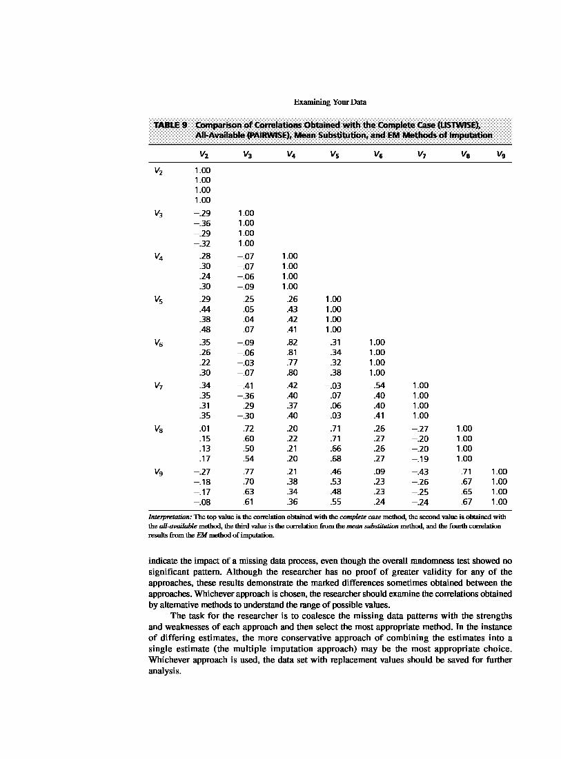
Examining Your Data

TABLE9 Comparison of Correlations Obtained with the Complete case (LISlWISE), All-Available (PAIRWISE), Mean Substitution, and EM Methods of Imputation

v2 v3 v4 Vs V& v7 Va Vg

v2 1.00 1.00 1.00 1.00

v3 -.29 1.00 -.36 1.00 -.29 1.00 -.32 1.00

v4 .28 -.07 1.00 .30 -.07 1.00 .24 -.06 1.00 .30 -.09 1.00

Vs .29 .25 .26 1.00 .44 .OS .43 1.00 .38 .04 .42 1.00 .48 .07 .41 1.00

v6 .35 -.09 .82 .31 1.00 .26 -.06 .81 .34 1.00 .22 -.03 .77 .32 1.00 .30 -.07 .80 .38 1.00

v7 .34 -.41 .42 -.03 .54 1.00 .35 -.36 .40 .07 .40 1.00 .31 -.29 .37 .06 .40 1.00 .35 -.30 .40 .03 .41 1.00

Va .01 .72 .20 .71 .26 -.27 1.00 .15 .60 .22 .71 .27 -.20 1.00 .13 .50 .21 .66 .26 -.20 1.00 .17 .54 .20 .68 .27 -.19 1.00

Vg -.27 .77 .21 .46 .09 -.43 .71 1.00 -.18 .70 .38 .53 .23 -.26 .67 1.00 -.17 .63 .34 .48 .23 -.25 .65 1.00 -.08 .61 .36 .55 .24 -.24 .67 1.00

Interpretation: The top value is the correlation obtained with the complete case method, the second value is obtained with the all-available method, the third value is the correlation from the mean substitution method, and the fourth correlation results from the EM method of imputation.

indicate the impact of a missing data process, even though the overall randomness test showed no significant pattern. Although the researcher has no proof of greater validity for any of the approaches, these results demonstrate the marked differences sometimes obtained between the approaches. Whichever approach is chosen, the researcher should examine the correlations obtained by alternative methods to understand the range of possible values.

The task for the researcher is to coalesce the missing data patterns with the strengths and weaknesses of each approach and then select the most appropriate method. In the instance of differing estimates, the more conservative approach of combining the estimates into a single estimate (the multiple imputation approach) may be the most appropriate choice. Whichever approach is used, the data set with replacement values should be saved for further analysis.

Examining Your Data

A RECAP OF THE MISSING VALUE ANALYSIS Evaluation of the issues surrounding missing data in the data set can be summarized in four conclusions:

1. The missing data process is MCAR. All of the diagnostic techniques support the conclusion that no systematic missing data process exists, making the missing data MCAR (missing completely at random). Such a finding provides two advantages to the researcher. First, it should not involve any hidden impact on the results that need to be considered when interpret­ing the results. Second, any of the imputation methods can be applied as remedies for the missing data. Their selection need not be based on their ability to handle nonrandom processes, but instead on the applicability of the process and its impact on the results.

2. Imputation is the most logical course of action. Even given the benefit of deleting cases and variables, the researcher is precluded from the simple solution of using the complete case method, because it results in an inadequate sample size. Some form of imputation is therefore needed to maintain an adequate sample size for any multivariate analysis.

3. Imputed correlations differ across techniques. When estimating correlations among the vari­ables in the presence of missing data, the researcher can choose from four commonly employed techniques: the complete case method, the all-available information method, the mean substitu­tion method, and the EM method. The researcher is faced in this situation, however, with differ­ences in the results among these methods. The all-available information, mean substitution, and EM approaches lead to generally consistent results. Notable differences, however, are found between these approaches and the complete information approach. Even though the complete information approach would seem the most "safe" and conservative, in this case it is not recom­mended due to the small sample used (only 26 observations) and its marked differences from the other two methods. The researcher should, if necessary, choose among the other approaches.

4. Multiple methods for replacing the missing data are available and appropriate. As already mentioned, mean substitution is one acceptable means of generating replacement values for the missing data. The researcher also has available the regression and EM imputa­tion methods, each of which give reasonably consistent estimates for most variables. The pres­ence of several acceptable methods also enables the researcher to combine the estimates into a single composite, hopefully mitigating any effects strictly due to one of the methods.

In conclusion, the analytical tools and the diagnostic processes presented in the earlier section provide an adequate basis for understanding and accommodating the missing data found in the pretest data. As this example demonstrates, the researcher need not fear that missing data will always preclude a multivariate analysis or always limit the generalizability of the results. Instead, the possibly hidden impact of missing data can be identified and actions taken to minimize the effect of missing data on the analyses performed.

OUTLIERS

Outliers are observations with a unique combination of characteristics identifiable as distinctly dif­ferent from the other observations. What constitutes a unique characteristic? Typically it is judged to be an unusually high or low value on a variable or a unique combination of values across several variables that make the observation stand out from the others. In assessing the impact of outliers, we must consider the practical and substantive considerations:

• From a practical standpoint, outliers can have a marked effect on any type of empirical analy­sis. For example, assume that we sample 20 individuals to determine the average household income. In our sample we gather responses that range between $20,000 and $100,000, so that the average is $45,000. But assume that the 21st person has an income of $1 million. H we include this value in the analysis, the average income increases to more than $90,000. Obviously, the outlier is a valid case, but what is the better estimate of the average household

Examining Your Data

income: $45,000 or $90,000? The researcher must assess whether the outlying value is retained or eliminated due to its undue influence on the results.

• In substantive terms, the outlier must be viewed in light of how representative it is of the population. Again, using our example of household income, how representative of the more wealthy segment is the millionaire? H the researcher feels that it is a small, but viable segment in the population, then perhaps the value should be retained. H, however, this millionaire is the only one in the entire population and truly far above everyone else (i.e., unique) and rep­resents an extreme value, then it may be deleted.

Outliers cannot be categorically characterized as either beneficial or problematic, but instead must be viewed within the context of the analysis and should be evaluated by the types of information they may provide. When beneficial, outliers-although different from the majority of the sample­may be indicative of characteristics of the population that would not be discovered in the normal course of analysis. In contrast, problematic outliers are not representative of the population, are counter to the objectives of the analysis, and can seriously distort statistical tests. Owing to the vary­ing impact of outliers, it is imperative that the researcher examine the data for the presence of outliers and ascertain their type of influence. Additionally, outliers should be placed in a framework particu­larly suited for assessing the influence of individual observations and determining whether this influ­ence is helpful or harmful.

Why do outliers occur? Outliers can be classified into one of four classes based on the source of their uniqueness:

• The first class arises from a procedural error, such as a data entry error or a mistake in coding. These outliers should be identified in the data cleaning stage, but if overlooked they should be eliminated or recorded as missing values.

• The second class of outlier is the observation that occurs as the result of an extraordinary event, which accounts for the uniqueness of the observation. For example, assume we are tracking average daily rainfall, when we have a hurricane that lasts for several days and records extremely high rainfall levels. These rainfall levels are not comparable to anything else recorded in the normal weather patterns. H included, they will markedly change the pattern of the results. The researcher must decide whether the extraordinary event fits the objectives of the research. H so, the outlier should be retained in the analysis. H not, it should be deleted.

• The third class of outlier comprises extraordinary observations for which the researcher has no explanation. In these instances, a unique and markedly different profile emerges. Although these outliers are the most likely to be omitted, they may be retained if the researcher feels they represent a valid element of the population. Perhaps they represent an emeiging element, or an untapped element previously not identified. Here the researcher must use judgment in the retention/deletion decision.

• The fourth and final class of outlier contains observations that fall within the ordinary range of values on each of the variables. These observations are not particularly high or low on the variables, but are unique in their combination of values across the variables. In these situ­ations, the researcher should retain the observation unless specific evidence is available that discounts the outlier as a valid member of the population.

Deteding and Handling Outliers

The following sections detail the methods used in detecting outliers in univariate, bivariate, and multivariate situations. Once identified, they may be profiled to aid in placing them into one of the four classes just described. Finally, the researcher must decide on the retention or exclusion of each outlier, judging not only from the characteristics of the outlier but also from the objectives of the analysis.

Examining Your Data

METHODS OF DETEcnNG OUTUERS Outliers can be identified from a univariate, bivariate, or multivariate perspective based on the number of variables (characteristics) considered. The researcher should utilize as many of these perspectives as possible, looking for a consistent pattern across perspectives to identify outliers. The following discussion details the processes involved in each of the three perspectives.

Univariate Detection. The univariate identification of outliers examines the distribution of observations for each variable in the analysis and selects as outliers those cases falling at the outer ranges (high or low) of the distribution. The primary issue is establishing the threshold for designa­tion of an outlier. The typical approach first converts the data values to standard scores, which have a mean of 0 and a standard deviation of 1. Because the values are expressed in a standardized format, comparisons across variables can be made easily.

In either case, the researcher must recognize that a certain number of observations may occur normally in these outer ranges of the distribution. The researcher should strive to identify only those truly distinctive observations and designate them as outliers.

Bivariate Detection. In addition to the univariate assessment, pairs of variables can be assessed jointly through a scat:terplot Cases that fall markedly outside the range of the other observations will be seen as isolated points in the scat:terplot Th assist in determining the expected range of observations in this two-dimensional portrayal, an ellipse representing a bivariate normal distribution's confidence interval (typically set at the 90% or 95% level) is superimposed over the scatterplot. This ellipse provides a graphical portrayal of the confidence limits and facilitates identification of the outliers. A variant of the scat:terplot is termed the influence plot, with each point varying in size in relation to its influence on the relationship.

Each of these methods provides an assessment of the uniqueness of each observation in rela­tionship to the other observation based on a specific pair of variables. A drawback of the bivariate method in general is the potentially large number of scatterplots that arise as the number of vari­ables increases. For three variables, it is only three graphs for all pairwise comparisons. But for five variables, it takes 10 graphs, and for 10 variables it takes 45 scatterplots! As a result, the researcher should limit the general use of bivariate methods to specific relationships between variables, such as the relationship of the dependent versus independent variables in regression. The researcher can then examine the set of scatterplots and identify any general pattern of one or more observations that would result in their designation as outliers.

Multivariate Detection. Because most multivariate analyses involve more than two vari­ables, the bivariate methods quickly become inadequate for several reasons. First, they require a large number of graphs, as discussed previously, when the number of variables reaches even mod­erate size. Second, they are limited to two dimensions (variables) at a time. Yet when more than two variables are considered, the researcher needs a means to objectively measure the multidimensional position of each observation relative to some common point. This issue is addressed by the Mahalanobis Jil measure, a multivariate assessment of each observation across a set of variables. This method measures each observation's distance in multidimensional space from the mean center of all observations, providing a single value for each observation no matter how many variables are considered. Higher Jil values represent observations farther removed from the general distribution of observations in this multidimensional space. This method, however, also has the drawback of only providing an overall assessment, such that it provides no insight as to which particular variables might lead to a high Jil value.

For interpretation purposes, the Mahalanobis Jil measure has statistical properties that allow for significance testing. The Jil measure divided by the number of variables involved (ff/dj) is approximately distributed as a t-value. Given the nature of the statistical tests, it is suggested that conservative levels of significance (e.g., .005 or .001) be used as the threshold value for designation as an outlier. Thus, observations having a ff/dfvalue exceeding 2.5 in small samples and 3 or 4 in

Examining Your Data

large samples can be designated as possible outliers. Once identified as a potential outlier on the Jil measure, an observation can be reexamined in terms of the univariate and bivariate methods discussed earlier to more fully understand the nature of its uniqueness.

OUTUER DESIGNATION With these univariate, bivariate, and multivariate diagnostic methods, the researcher has a complementary set of perspectives with which to examine observations as to their status as outliers. Each of these methods can provide a unique perspective on the observations and be used in a concerted manner to identify outliers (see Rules of Thumb 4).

When observations have been identified by the univariate, bivariate, and multivariate methods as possible outliers, the researcher must then select only observations that demonstrate real unique­ness in comparison with the remainder of the population across as many perspectives as possible. The researcher must refrain from designating too many observations as outliers and not succumb to the temptation of eliminating those cases not consistent with the remaining cases just because they are different.

OUTLIER DESCRIPTION AND PROFILING Once the potential outliers are identified, the researcher should generate profiles of each outlier observation and identify the variable(s) responsi­ble for its being an outlier. In addition to this visual examination, the researcher can also employ multivariate techniques such as discriminant analysis or multiple regression to identify the differ­ences between outliers and the other observations. H possible the researcher should assign the out­lier to one of the four classes described earlier to assist in the retention or deletion decision to be made next. The researcher should continue this analysis until satisfied with understanding the aspects of the case that distinguish the outlier from the other observations.

RETENTION OR DELETION OF THE OUTLIER After the outliers are identified, profiled, and categorized, the researcher must decide on the retention or deletion of each one. Many philoso­phies among researchers offer guidance as to how to deal with outliers. Our belief is that they should be retained unless demonstrable proof indicates that they are truly aberrant and not representative of any observations in the population. If they do portray a representative element or segment of the population, they should be retained to ensure generalizability to the entire population. As outliers are deleted, the researcher runs the risk of improving the multivariate analysis but limiting its generalizability. H outliers are problematic in a particular technique,

RULES OF THUMB 4

Outlier Detection

• Univariate methods: Examine all metric variables to identify unique or extreme observations • For small samples (80 or fewer observations), outliers typically are defined as cases with

standard scores of 2.5 or greater • For larger sample sizes, increase the threshold value of standard scores up to 4 • If standard scores are not used, identify cases falling outside the ranges of 2.5 versus 4 standard

deviations, depending on the sample size

• Bivariate methods: Focus their use on specific variable relationships, such as the independent versus dependent variables • Use scatterplots with confidence intervals at a specified alpha level

• Multivariate methods: Best suited for examining a complete variate, such as the independent variables in regression or the variables in factor analysis • Threshold levels for the filtdfmeasure should be conservative (.DOS or .001), resulting in values

of 2.5 (small samples) versus 3 or 4 in larger samples

Examining Your Data

many times they can be accommodated in the analysis in a manner in which they do not seri­ously distort the analysis.

An Illustrative Example of Analyzing Outliers

As an example of outlier detection, the observations of an HBAT database are examined for out­liers. The variables considered in the analysis are the metric variables X6 through X19, with the context of our examination being a regression analysis, where X19 is the dependent variable and X6 through X18 are the independent variables. The outlier analysis will include univariate, bivari­ate, and multivariate diagnoses. When candidates for outlier designation are found, they are examined, and a decision on retention or deletion is made.

OUTUER DETECTION The first step is examination of all the variables from a univariate perspec­tive. Bivariate methods will then be employed to examine the relationships between the dependent variable (X19) and each of the independent variables. From each of these scattetplots, observations that fall outside the typical distribution can be identified and their impact on that relationship ascer­tained. Finally, a multivariate assessment will be made on all of the independent variables collec­tively. Comparison of observations across the three methods will hopefully provide the basis for the deletion/retention decision.

Univariate Detection. The first step is to examine the observations on each of the vari­ables individually. Table 10 contains the observations with standardized variable values exceeding ±2.5 on each of the variables (X6 to X19). From this univariate perspective, only observations 7, 22, and 90 exceed the threshold on more than a single variable. Moreover, none of these observa­tions had values so extreme as to affect any of the overall measures of the variables, such as the mean or standard deviation. We should note that the dependent variable had one outlying observa­tion (22), which may affect the bivariate scattetplots because the dependent variable appears in each

TABLE 10 Univariate. Bivariate. and Multivariate Outlier Detection Results

UNIVARIATE OUTLIERS BIVARIATE OUTLIERS

Cases with Standardized Values Cases Outside the 95%

Exceeding ± 2.5 Confidence Interval Ellipse

X19 with:

x6 No cases x6 44,90 x7 13,22,90 x7 13,22,24,53,90 X a 8, 7 X a 22,87 Xg No cases Xg 2,22,45,52 xlO No cases xlO 22,24,85 xll 7 xll 2, 7,22,45 X12 90 X12 22,44,90 x13 No cases x13 22,57 X14 77 X14 22,77,84 X1s 6,53 X1s 6,22,53 X16 24 X16 22,24,48,62,92 Xn No cases Xn 22 X1a 7,84 X1a 2, 7,22,84 X19 22

aMahalanobis IY value based on the 13 HBAT peir:eptions (Xj, to X11J.

MULTIVARIATE OUTLIERS

Cases with a Value of D2/df Greater than 2.5

(df= 13)a

Case

98 36

40.0 36.9

ol!df

3.08 2.84

Examining Your Data

scatterplot. The three observations will be noted to see whether they appear in the subsequent bivariate and multivariate assessments.

Bivariate Detection. For a bivariate perspective, 13 scatterplots are formed for each of the independent variables (X6 through X18) with the dependent variable (X19). An ellipse representing the 95% confidence interval of a bivariate normal distribution is then superimposed on the scatter­plot. Figure 5 contains examples of two such scatterplots involving X6 and X7. As we can see in the scatterplot for X6 with X 19, the two outliers fall just outside the ellipse and do not have the most extreme values on either variable. This result is in contrast to the scatterplot of X7 with X19, where observation 22 is marlredly different from the other observations and shows the highest values on both X7 and X19. The second part of Table 10 contains a compilation of the observations falling outside this ellipse for each variable. Because it is a 95% confidence interval, we would expect some observations normally to fall outside the ellipse. Only four observations (2, 22, 24, and 90) fall outside the ellipse more than two times. Observation 22 falls outside in 12 of the 13 scatterplots, mostly because it is an outlier on the dependent variable. Of the remaining three observations, only observation 90 was noted in the univariate detection.

Multivariate Detection. The final diagnostic method is to assess multivariate outliers with the Maha1anobis Jil measure (see Table 10). This analysis evaluates the position of each observation com­pared with the center of all observations on a set of variables. In this case, all the metric independent

11

10 • 9

... t : I ... . .

• . . . 8 .

I . >< .. . . . . . .

7 • • . ' . • . . ..

6

5

4 4 5 6 7 8 9 10

X19

6

••

5

. . >< 4 .. . . . . . -· ·' . . • . •• . . .. . • .. . .. . • • •• . . .

3 .. • 2

4 5 6 7 8 9 10

X19

Examining Your Data

variables were used. The calculation of the U/dfvalue (df = 13) allows for identification of outliers through an approximate test of statistical significance. Because the sample has only 100 observations, a threshold value of 2.5 will be used rather than the value of 3.5 or 4.0 used in latge samples. With this threshold, two observations (98 and 36) are identified as significantly different It is interesting that these observations were not seen in earlier univariate and bivariate analyses but appear only in the multivariate tests. This result indicates they are not unique on any single variable but instead are unique in combination.

RETENTION OR DEI..ET10N OF THE OUTUERS As a result of these diagnostic tests, no observa­tions demonstrate the characteristics of outliers that should be eliminated. Each variable has some observations that are extreme, and they should be considered if that variable is used in an analysis. No observations are extreme on a sufficient number of variables to be considered unrepresentative of the population. In all instances, the observations designated as outliers, even with the multivari­ate tests, seem similar enough to the remaining observations to be retained in the multivariate analyses. However, the researcher should always examine the results of each specific multivariate technique to identify observations that may become outliers in that particular application.

TESTING THE ASSUMPTIONS OF MULTIVARIATE ANALYSIS

The final step in examining the data involves testing for the assumptions underlying the statisti­cal bases for multivariate analysis. The earlier steps of missing data analysis and outlier detec­tion attempted to clean the data to a format most suitable for multivariate analysis. Testing the data for compliance with the statistical assumptions underlying the multivariate techniques now deals with the foundation upon which the techniques make statistical inferences and results. Some techniques are less affected by violating certain assumptions, which is termed robustness, but in all cases meeting some of the assumptions will be critical to a successful analysis. Thus, it is necessary to understand the role played by each assumption for every multivariate technique.

The need to test the statistical assumptions is increased in multivariate applications because of two characteristics of multivariate analysis. First, the complexity of the relationships, owing to the typical use of a latge number of variables, makes the potential distortions and biases more potent when the assumptions are violated, particularly when the violations compound to become even more detrimental than if considered separately. Second, the complexity of the analyses and results may mask the indicators of assumption violations apparent in the simpler univariate analyses. In almost all instances, the multivariate procedures will estimate the multivariate model and pro­duce results even when the assumptions are severely violated. Thus, the researcher must be aware of any assumption violations and the implications they may have for the estimation process or the interpretation of the results.

Assessing Individual Variables Versus the Variate

Multivariate analysis requires that the assumptions underlying the statistical techniques be tested twice: first for the separate variables, akin to the tests for a univariate analysis, and second for the multivariate model variate, which acts collectively for the variables in the analysis and thus must meet the same assumptions as individual variables. This chapter focuses on the examination of indi­vidual variables for meeting the assumptions underlying the multivariate procedures. Discussions in this chapter address the methods used to assess the assumptions underlying the variate for each multivariate technique.

Examining Your Data

Four Important Statistical Assumptions

Multivariate techniques and their univariate counterparts are all based on a fundamental set of assump­tions representing the requirements of the underlying statistical theory. Although many assumptions or requirements come into play in one or more of the multivariate techniques, four of them potentially affect every univariate and multivariate statistical technique.

NORMAUTY The most fundamental assumption in multivariate analysis is normality, referring to the shape of the data distribution for an individual metric variable and its correspondence to the normal distribution, the benchmark for statistical methods. If the variation from the normal distri­bution is sujjiciently large, all resulting statistical tests are invalid, because normality is required to use the F and t statistics. Both the univariate and the multivariate statistical methods discussed in this text are based on the assumption of univariate normality, with the multivariate methods also assuming multivariate normality.

Univariate normality for a single variable is easily tested, and a number of corrective meas­ures are possible, as shown later. In a simple sense, multivariate normality (the combination of two or more variables) means that the individual variables are normal in a univariate sense and that their combinations are also normal. Thus, if a variable is multivariate normal, it is also uni­variate normal. However, the reverse is not necessarily true (two or more univariate normal vari­ables are not necessarily multivariate normal). Thus, a situation in which all variables exhibit univariate normality will help gain, although not guarantee, multivariate normality. Multivariate normality is more difficult to test [13, 23], but specialized tests are available in the techniques most affected by departures from multivariate normality. In most cases assessing and achieving univariate normality for all variables is sufficient, and we will address multivariate normality only when it is especially critical. Even though large sample sizes tend to diminish the detrimen­tal effects of nonnormality, the researcher should always assess the normality for all metric vari­ables included in the analysis.

Assessing the Impact of Violating the Normality Assumption. The severity of nonnormal­ity is based on two dimensions: the shape of the offending distribution and the sample size. As we will see in the following discussion, the researcher must not only judge the extent to which the variable's distribution is nonnormal, but also the sample sizes involved. What might be considered unacceptable at small sample sizes will have a negligible effect at larger sample sizes.

Impacts Due to the Shape of the Distribution. How can we describe the distribution if it differs from the normal distribution? The shape of any distribution can be described by two meas­ures: kurtosis and skewness. Kurtosis refers to the "peakedness" or ''flatness" of the distribution compared with the normal distribution. Distributions that are taller or more peaked than the normal distribution are termed leptokurtic, whereas a distribution that is flatter is termed platykurtic. Whereas kurtosis refers to the height of the distribution, skewness is used to describe the balance of the distribution; that is, is it unbalanced and shifted to one side (right or left) or is it centered and symmetrical with about the same shape on both sides? H a distribution is unbalanced, it is skewed. A positive skew denotes a distribution shifted to the left, whereas a negative skewness reflects a shift to the right

Knowing how to describe the distribution is followed by the issue of how to determine the extent or amount to which it differs on these characteristics? Both skewness and kurtosis have empirical measures that are available in all statistical programs. In most programs, the skewness and kurtosis of a normal distribution are given values of zero. Then, values above or below zero denote departures from normality. For example, negative kurtosis values indicate a platykurtic (flatter) distribution, whereas positive values denote a leptokurtic (peaked) distribution. Likewise, positive skewness values indicate the distribution shifted to the left, and the negative values denote a rightward shift. To judge the ''Are they large enough to worry aboutT' question for these values,

Examining Your Data

the following discussion on statistical tests shows how the kurtosis and skewness values can be transformed to reflect the statistical significance of the differences and provide guidelines as to their severity.

Impacts Due to Sample Size. Even though it is important to understand how the distribu­tion departs from normality in terms of shape and whether these values are large enough to war­rant attention, the researcher must also consider the affects of sample size. Sample size has the effect of increasing statistical power by reducing sampling error. It results in a similar effect here, in that larger sample sizes reduce the detrimental effects of nonnormality. In small samples of 50 or fewer observations, and especially if the sample size is less than 30 or so, significant depar­tures from normality can have a substantial impact on the results. For sample sizes of 200 or more, however, these same effects may be negligible. Moreover, when group comparisons are made, such as in AN OVA, the differing sample sizes between groups, if large enough, can even cancel out the detrimental effects. Thus, in most instances, as the sample sizes become large, the researcher can be less concerned about nonnormal variables, except as they might lead to other assumption violations that do have an impact in other ways (e.g., see the following discussion on homoscedasticity ).

Graphical Analyses of Normality. The simplest diagnostic test for normality is a visual check of the histogram that compares the observed data values with a distribution approximating the normal distribution (see Figure 1). Although appealing because of its simplicity, this method is problematic for smaller samples, where the construction of the histogram (e.g., the number of categories or the width of categories) can distort the visual portrayal to such an extent that the analysis is useless. A more reliable approach is the normal probability plot, which compares the cumulative distribution of actual data values with the cumulative distribution of a normal distribu­tion. The normal distribution forms a straight diagonal line, and the plotted data values are com­pared with the diagonal. H a distribution is normal, the line representing the actual data distribution closely follows the diagonal.

Figure 6 shows several departures from normality and their representation in the normal probability in terms of kurtosis and skewness. First, departures from the normal distribution in terms of kurtosis are easily seen in the normal probability plots. When the line falls below the diagonal, the distribution is flatter than expected. When it goes above the diagonal, the distribu­tion is more peaked than the normal curve. For example, in the normal probability plot of a peaked distribution (Figure 6d), we see a distinct S-shaped curve. Initially the distribution is flatter, and the plotted line falls below the diagonal. Then the peaked part of the distribution rap­idly moves the plotted line above the diagonal, and eventually the line shifts to below the diago­nal again as the distribution flattens. A nonpeaked distribution has the opposite pattern (Figure 6c). Skewness is also easily seen, most often represented by a simple arc, either above or below the diagonal. A negative skewness (Figure 6e) is indicated by an arc below the diagonal, whereas an arc above the diagonal represents a positively skewed distribution (Figure 6f). An excellent source for interpreting normal probability plots, showing the various patterns and interpretations, is Daniel and Wood [7]. These specific patterns not only identify nonnormality but also tell us the form of the original distribution and the appropriate remedy to apply.

Statistical Tests of Normality. In addition to examining the normal probability plot, one can also use statistical tests to assess normality. A simple test is a rule of thumb based on the skewness and kurtosis values (available as part of the basic descriptive statistics for a variable computed by all statistical programs). The statistic value (z) for the skewness value is calculated as:

skewness Z skewness = ----= {6=--

\f~

Normal Univariate probability plot distribution

. .

(a) Normal distribution

. .

Normal Univariate probability plot distribution

. .

(c) Nonpeaked distribution

. . .

Normal Univariate probability plot distribution

(e) Negative distribution

Plot of univariate distribution

Examining Your Data

. .

Normal Univariate probability plot distribution

(b) Uniform distribution

. . .

!\ Normal Univariate

probability plot distribution

(d) Peaked distribution

. . . .

Normal Univariate probability plot distribution

(f) Positive distribution

Cumulative normal distribution

RGURE 6 Nonnal Probabili'l;y Plots and Corresponding Univariate Distributions

where N is the sample size. A z value can also be calculated for the kurtosis value using the following formula:

kurtosis z kurtosis = !J

If either calculated z value exceeds the specified critical value, then the distribution is nonnormal in terms of that characteristic. The critical value is from a z distribution, based on the significance level we desire. The most commonly used critical values are ±2.58 (.0 1 significance level) and ±1.96, which corresponds to a .05 error level. With these simple tests, the researcher can easily assess the degree to which the skewness and peakedness of the distribution vary from the normal distribution.

Specific statistical tests for normality are also available in all the statistical programs. The two most common are the Shapiro-Wilks test and a modification of the Kolmogorov-Smimov test. Each calculates the level of significance for the differences from a normal distribution. The researcher

Examining Your Data

should always remember that tests of significance are less useful in small samples (fewer than 30) and quite sensitive in large samples (exceeding 1,000 observations). Thus, the researcher should always use both the graphical plots and any statistical tests to assess the actual degree of departure from normality.

Remedies for Nonnormality. A number of data transformations available to accommodate nonnormal distributions are discussed later in the chapter. This chapter confines the discussion to uni­variate normality tests and transformations. However, when we examine other multivariate methods, such as multivariate regression or multivariate analysis of variance, we discuss tests for multivariate normality as well. Moreover, many times when nonnormality is indicated, it also contributes to other assumption violations; therefore, remedying normality first may assist in meeting other statistical assumptions as well. (For those interested in multivariate normality, see references [13, 16, 25].)

HOMOSCEDASTICITY The next assumption is related primarily to dependence relationships between variables. Homoscedasticity refers to the assumption that dependent variable(s) exhibit equal levels of variance across the range of predictor variable(s). Homoscedasticity is desirable because the variance of the dependent variable being explained in the dependence relationship should not be concentrated in only a limited range of the independent values. In most situations, we have many different values of the dependent variable at each value of the independent variable. For this relationship to be fully captured, the dispersion (variance) of the dependent variable values must be relatively equal at each value of the predictor variable. H this dispersion is unequal across values of the independent variable, the relationship is said to be heteroscedastic. Although the dependent variables must be metric, this concept of an equal spread of variance across independent variables can be applied when the independent variables are either metric or nonmetric:

• Metric independent variables. The concept of homoscedasticity is based on the spread of dependent variable variance across the range of independent variable values, which is encoun­tered in techniques such as multiple regression. The dispersion of values for the dependent variable should be as large for small values of the independent values as it is for moderate and large values. In a scatterplot, it is seen as an elliptical distribution of points

• Nonmetric independent variables. In these analyses (e.g., ANOVA and MANOVA) the focus now becomes the equality of the variance (single dependent variable) or the variance/covari­ance matrices (multiple dependent variables) across the groups formed by the nonmetric inde­pendent variables. The equality of variance/covariance matrices is also seen in discriminant analysis, but in this technique the emphasis is on the spread of the independent variables across the groups formed by the nonmetric dependent measure.

In each of these instances, the purpose is the same: to ensure that the variance used in expla­nation and prediction is distributed across the range of values, thus allowing for a ''fair test" of the relationship across all values of the nonmetric variables. The two most common sources of heteroscedasticity are the following:

• Variable type. Many types of variables have a natural tendency toward differences in disper­sion. For example, as a variable increases in value (e.g., units ranging from near zero to millions) a naturally wider range of answers is possible for the larger values. Also, when percentages are used the natural tendency is for many values to be in the middle range, with few in the lower or higher values.

• Skewed distribution of one or both variables. In Figure 7a, the scatterplots of data points for two variables (V1 and V~ with normal distributions exhibit equal dispersion across all data values (i.e., homoscedasticity). However, in Figure 7b we see unequal dispersion (heteroscedasticity) caused by skewness of one of the variables (V3). For the different values of V3, there are different patterns of dispersion for V1.

. . •• . . , .. : '• , ·:F$.

' .... I • • -~"··' t,• ••• . , .. ,.

.. • .r ... . . ·' ..

vl (a) Homoscedasticity

Examining Your Data

. . . . . : .. . ... ~. ' . ... '" . ..,.. . . •. : .. .:tt;•

' , •• _, •t. • • - I ...... ·' • • r: . ..... : . '··· . ... . .

vl

•

(b) Heteroscedasticity

FIGURE 7 Scatterplats af Hamasa!dastic and Heterascedastic: Relationships

The result of heteroscedasticity is to cause the predictions to be better at some levels of the independent variable than at others. This variability affects the standard errors and makes hypothe­sis tests either too stringent or too insensitive. The effect of heteroscedasticity is also often related to sample size, especially when examining the variance dispersion across groups. For example, in ANOVA or MANOVA the impact ofheteroscedasticity on the statistical test depends on the sample sizes associated with the groups of smaller and larger variances. In multiple regression analysis, similar effects would occur in highly skewed distributions where there were disproportionate num­bers of respondents in certain ranges of the independent variable.

Graphical Tests of Equal Variance Dispersion. The test of homoscedasticity for two metric variables is best examined graphically. Departures from an equal dispersion are shown by such shapes as cones (small dispersion at one side of the graph, large dispersion at the opposite side) or diamonds (a large number of points at the center of the distribution). The most common application of graphical tests occurs in multiple regression, based on the dispersion of the dependent variable across the values of either the metric independent variables.

Boxplots work well to represent the degree of variation between groups formed by a categor­ical variable. The length of the box and the whiskers each portray the variation of data within that group. Thus, heteroscedasticity would be portrayed by substantial differences in the length of the boxes and whiskers between groups representing the dispersion of observations in each group.

Statistical Tests for Homoscedasticity. The statistical tests for equal variance dispersion assess the equality of variances within groups formed by nonmetric variables. The most common test, the Levene test, is used to assess whether the variances of a single metric variable are equal across any number of groups. H more than one metric variable is being tested, so that the compari­son involves the equality of variance/covariance matrices, the Box's M test is applicable. The Box's M test is available in both multivariate analysis of variance and discriminant analysis.

Remedies for Heteroscedasticity. Heteroscedastic variables can be remedied through data transformations similar to those used to achieve normality. As mentioned earlier, many times het­eroscedasticity is the result of nonnormality of one of the variables, and correction of the nonnor­mality also remedies the unequal dispersion of variance. A later section discusses data

Examining Your Data

transformations of the variables to "spread" the variance and make all values have a potentially equal effect in prediction.

LINEARITY An implicit assumption of all multivariate techniques based on correlational measures of association, including multiple regression, logistic regression, factor analysis, and structural equation modeling, is linearity. Because correlations represent only the linear association between variables, nonlinear effects will not be represented in the correlation value. This omission results in an underestimation of the actual strength of the relationship. It is always prudent to examine all rela­tionships to identify any departures from linearity that may affect the correlation.

Identifying Nonlinear Relationships. The most common way to assess linearity is to examine scatterplots of the variables and to identify any nonlinear patterns in the data. Many scatterplot pro­grams can show the straight line depicting the linear relationship, enabling the researcher to better identify any nonlinear characteristics. An alternative approach is to run a simple regression analysis and to examine the residuals. The residuals reflect the unexplained portion of the dependent variable; thus, any nonlinear portion of the relationship will show up in the residuals. A thinl approach is to explicitly model a nonlinear relationship by the testing of alternative model specifications (also know as curve fitting) that reflect the nonlinear elements.

Remedies for Nonlinearity. H a nonlinear relationship is detected, the most direct approach is to transform one or both variables to achieve linearity. A number of available transformations are discussed later in this chapter. An alternative to data transformation is the creation of new variables to represent the nonlinear portion of the relationship.

ABSENCE OF CORRELATED ERRORS Predictions in any of the dependence techniques are not per­fect, and we will rarely find a situation in which they are. However, we do attempt to ensure that any prediction errors are uncorrelated with each other. For example, if we found a pattern that suggests every other error is positive while the alternative error terms are negative, we would know that some unexplained systematic relationship exists in the dependent variable. H such a situation exists, we cannot be confident that our prediction errors are independent of the levels at which we are trying to predict. Some other factor is affecting the results, but is not included in the analysis.

Identifying Correlated Errors. One of the most common violations of the assumption that errors are uncorrelated is due to the data collection process. Similar factors that affect one group may not affect the other. H the groups are analyzed separately, the effects are constant within each group and do not impact the estimation of the relationship. But if the observations from both groups are combined, then the final estimated relationship must be a compromise between the two actual relationships. This combined effect leads to biased results because an unspecified cause is affecting the estimation of the relationship.

Another common source of correlated errors is time series data. As we would expect, the data for any time period is highly related to the data at time periods both before and afterward. Thus, any predic­tions and any prediction errors will necessarily be correlated. This type of data led to the creation of spe­cialized programs specifically for time series analysis and this pattern of correlated observations.

To identify correlated errors, the researcher must first identify possible causes. Values for a variable should be grouped or ordered on the suspected variable and then examined for any patterns. In our earlier example of grouped data, once the potential cause is identified the researcher could see whether differences did exist between the groups. Finding differences in the prediction errors in the two groups would then be the basis for determining that an unspecified effect was "causing" the correlated errors. For other types of data, such as time series data, we can see any trends or patterns when we order the data (e.g., by time period for time series data). This ordering variable (time in

Examining Your Data

this case), if not included in the analysis in some manner, would cause the errors to be correlated and create substantial bias in the results.

Remedies for Correlated Errors. Correlated errors must be corrected by including the omit­ted causal factor into the multivariate analysis. In our earlier example, the researcher would add a variable indicating in which class the respondents belonged. The most common remedy is the addi­tion of a variable(s) to the analysis that represents the omitted factor. The key task facing the researcher is not the actual remedy, but rather the identification of the unspecified effect and a means of representing it in the analysis.

OVERVIEW OF TESTING FOR STATISTICAL ASSUMPTIONS The researcher is faced with what may seem to be an impossible task: satisfy all of these statistical assumptions or risk a biased and flawed analysis. We want to note that even though these statistical assumptions are important, the researcher must use judgment in how to interpret the tests for each assumption and when to apply remedies. Even analyses with small sample sizes can withstand small, but significant, departures from normality. What is more important for the researcher is to understand the implications of each assumption with reganl to the technique of interest, striking a balance between the need to satisfy the assumptions versus the robustness of the technique and research context. The following guide­lines in Rules of Thumb 5 attempt to portray the most pragmatic aspects of the assumptions and the reactions that can be taken by researchers.

Data Transfonnations

Data transformations provide a means of modifying variables for one of two reasons: (1) to cor­rect violations of the statistical assumptions underlying the multivariate techniques or (2) to improve the relationship (correlation) between variables. Data transformations may be based on reasons that are either theoretical (transformations whose appropriateness is based on the nature of the data) or data derived (where the transformations are suggested strictly by an examination of the data). Yet in either case the researcher must proceed many times by trial and error, monitoring the improvement versus the need for additional transformations.

All the transformations described here are easily carried out by simple commands in the popular statistical packages. We focus on transformations that can be computed in this man­ner, although more sophisticated and complicated methods of data transformation are available (e.g., see Box and Cox [3]).

RULES OF THUMB 5

Testing Statistical Assumptions

• Normality can have serious effects in small samples (fewer than 50 cases), but the impact effec­tively diminishes when sample sizes reach 200 cases or more

• Most cases of heteroscedasticity are a result of nonnormality in one or more variables; thus, remedying normality may not be needed due to sample size, but may be needed to equalize the variance

• Nonlinear relationships can be well defined, but seriously understated unless the data are transformed to a linear pattern or explicit model components are used to represent the nonlinear portion of the relationship

• Correlated errors arise from a process that must be treated much like missing data; that is, the researcher must first define the causes among variables either internal or external to the dataset; if they are not found and remedied, serious biases can occur in the results, many times unknown to the researcher

Examining Your Data

TRANSFORMATIONS TO ACHIEVE NORMALITY AND HOMOSCEDASTICTY Data transforma­tions provide the principal means of correcting nonnormality and heteroscedasticity. In both instances, patterns of the variables suggest specific transformations. For nonnormal distributions, the two most common patterns are flat distributions and skewed distributions. For the flat distribu­tion, the most common transformation is the inverse (e.g., 1/Y or 1/X). Skewed distributions can be transformed by taking the square root, logarithms, squared, or cubed (X2 or X3

) terms or even the inverse of the variable. Usually negatively skewed distributions are best transformed by employing a squared or cubed transformation, whereas the logarithm or square root typically works best on positive skewness. In many instances, the researcher may apply all of the possible transformations and then select the most appropriate transformed variable.

Heteroscedasticity is an associated problem, and in many instances "curing" this problem will deal with normality problems as well. Heteroscedasticity is also due to the distribution of the vari­able(s). When examining the scatterplot, the most common pattern is the cone-shaped distribution. H the cone opens to the right, take the inverse; if the cone opens to the left, take the square root. Some transformations can be associated with certain types of data. For example, frequency counts suggest a square root transformation; proportions are best transformed by the arcsin transformation

(xiii!W = 2 arcsin~); and proportional change is best handled by taking the logarithm of

the variable. In all instances, once the transformations have been performed, the transformed data should be tested to see whether the desired remedy was achieved.

TRANSFORMATIONS TO ACHIEVE LINEARITY Numerous procedures are available for achieving linearity between two variables, but most simple nonlinear relationships can be placed in one of four categories (see Figure 8). In each quadrant, the potential transformations for both dependent

y :z y

y

(a)

(b)

y

(c)

(d)

Source: F. Mosteller and J. W. Tukey, Data Analysis and Regression. Reading, MA: Addison-Wesley, 1977.

Examining Your Data

and independent variables are shown. For example, if the relationship looks like Figure 8a, then either variable can be squared to achieve linearity. When multiple transformation possibilities are shown, start with the top method in each quadrant and move downward until linearity is achieved. An alternative approach is to use additional variables, termed polynomials, to represent the nonlin­ear components.

GENERAL GUIDEUNES FOR TRANSFORMATIONS Many possibilities exist for transforming the data to achieve the required statistical assumptions. Apart from the technical issues of the type of transformation, several points to remember when performing data transformations are presented in Rules of Thumb 6.

An Illustration of Testing the Assumptions Underlying Multivariate Analysis

To illustrate the techniques involved in testing the data for meeting the assumptions underlying multivariate analysis and to provide a foundation for use of the data, the data set from the HBAT database will be examined. In the course of this analysis, the assumptions of normality, homoscedasticity, and linearity will be covered. The fourth basic assumption, the absence of cor­related errors, can be addressed only in the context of a specific multivariate model. Emphasis will be placed on examining the metric variables, although the nonmetric variables will be assessed where appropriate.

NORMALITY The assessment of normality of the metric variables involves both empirical measures of a distribution's shape characteristics (skewness and kurtosis) and the normal proba­bility plots. The empirical measures provide a guide as to the variables with significant devia­tions from normality, and the normal probability plots provide a visual portrayal of the shape of the distribution. The two portrayals complement each other when selecting the appropriate transformations.

Table 11 and Figure 9 contain the empirical measures and normal probability plots for the metric variables in our data set. Our first review concerns the empirical measures reflecting the shape of the distribution (skewness and kurtosis) as well as a statistical test for normality (the

RULES OF THUMB 6

Transforming Data

• To judge the potential impact of a transformation, calculate the ratio of the variable's mean to its standard deviation: • Noticeable effects should occur when the ratio is less than 4 • When the transformation can be performed on either of two variables, select the variable with

the smallest ratio

• Transformations should be applied to the independent variables except in the case of het­eroscedasticity

• Heteroscedasticity can be remedied only by the transformation of the dependent variable in a dependence relationship; if a heteroscedastic relationship is also nonlinear, the dependent vari­able, and perhaps the independent variables, must be transformed

• Transformations may change the interpretation of the variables; for example, transforming variables by taking their logarithm translates the relationship into a measure of proportional change (elasticity); always be sure to explore thoroughly the possible interpretations of the transformed variables

• Use variables in their original (untransformed) format when profiling or interpreting results

TABLE 11 Distributional Characteristics, 'R!sting for Normality, and Possible Remedies

SHAPE DESCRIPTORS

Skewness Kurtosis Tests of Normality Applicable Remedies

Description of the Significance Variable Statistic zvalue Statistic zvalue Statistic Significance Distribution Transformation After Remedy

Firm Characteristics

x6 -.245 -1.01 -1.132 -2.37 .109 .005 Almost uniform Squared term .015 distribution

X7 .660 2.74 .735 1.54 .122 .001 Peaked with Logarithm .037 positive skew

X a -.203 -.84 -.548 -1.15 .060 .2ooa Normal distribution Xg -.136 -.56 -.586 -1.23 .051 .2ooa Normal distribution x,o .044 .18 -.888 -1.86 .065 .200a Normal distribution x,, -.092 -.38 -.522 -1.09 .060 .2ooa Normal distribution x12 .377 1.56 .410 .86 .111 .004 Slight positive skew None

and peakedness x,3 -.240 -1.00 -.903 -1.89 .106 .007 Peaked Cubed term .022 x,4 .008 .03 -.445 -.93 .064 .2ooa Normal distribution x,s .299 1.24 .016 .03 .074 .2ooa Normal distribution x,6 -.334 -1.39 .244 .51 .129 .000 Negative skewness Squared term .066 x11 .323 1.34 -.816 -1.71 .1 01 .013 Peaked, positive Inverse .187

skewness x,s -.463 -1.92 .218 .46 .084 .082 Normal distribution

Performance Measures

X,g .078 .32 -.791 -1.65 .078 .137 Normal distribution X2o .044 .18 -.089 -.19 .077 .147 Normal distribution X21 -.093 -.39 -.090 -.19 .073 .2ooa Normal distribution X22 -.132 -.55 -.684 -1.43 .075 .180 Normal distribution

"Lower bound of true significance.

Note: The z values are derived by dividing the statistics by the appropriate standard errors of .241 (skewness) and .478 (kurtosis). The equations for calculating the standard errors are given in the text.

Examining Your Data

1.00 1.00

• • .75 . 75 . . .. . . .50 .50

25 25

0.00 0.00 0.00 25 .50 .75 1.00 0.00 25 .50 .75 1.00

~ Product Quality X7 E-Commerce Activities

1.00 1.00

.75 .75

.50 .50

25 25

• 0.00 0.00

0.00 25 .50 .75 1.00 0.00 25 .50 .75 1.00 X 12 Salesforce Image X 13 Competitive Pricing

1.00 1.00

.75 .75

.50 .50

25 25

0.00 0.00 0.00 25 .50 .75 1.00 0.00 25 .50 .75 1.00

X16 Order & Billing x17 Price Flexibility

modified Kolmogorov-Smimov test). Of the 17 metric variables, only 6 (X6, X7, X12, X13, X16, and X17) show any deviation from normality in the overall normality tests. When viewing the shape characteristics, significant deviations were found for skewness (X7) and kurtosis (A{;). One should note that only two variables were found with shape characteristics significantly different from the normal curve, while six variables were identified with the overall tests. The overall test provides no insight as to the transformations that might be best, whereas the shape characteristics provide guide­lines for possible transformations. The researcher can also use the normal probability plots to iden­tify the shape of the distribution. Figure 9 contains the normal probability plots for the six

Examining Your Data

variables found to have the nonnormal distributions. By combining information, from the empirical and graphical methods, the researcher can characterize the nonnormal distribution in anticipation of selecting a transformation (see Table 11 for a description of each nonnormal distribution).

Table 11 also suggests the appropriate remedy for each of the variables. Two variables (X6 and X16) were transformed by taking the square root. X7 was transformed by logarithm, whereas X17 was squared and X13 was cubed. Only X12 could not be transformed to improve on its distributional characteristics. For the other five variables, their tests of normality were now either nonsignificant (X16 and X17) or markedly improved to more acceptable levels (X6, X7,

and X13). Figure 10 demonstrates the effect of the transformation on X17 in achieving normal­ity. The transformed X17 appears markedly more normal in the graphical portrayals, and the statistical descriptors are also improved. The researcher should always examine the transformed variables as rigorously as the original variables in terms of their normality and distribution shape.

In the case of the remaining variable (X12), none of the transformations could improve the normality. This variable will have to be used in its original form. In situations where the normality of the variables is critical, the transformed variables can be used with the assurance that they meet the assumptions of normality. But the departures from normality are not so extreme in any of the original variables that they should never be used in any analysis in their original form. H the tech­nique has a robustness to departures from normality, then the original variables may be preferred for the comparability in the interpretation phase.

HOMOSCEDASTICITY All statistical packages have tests to assess homoscedasticity on a univari­ate basis (e.g., the Levene test in SPSS) where the variance of a metric variable is compared across levels of a nonmetric variable. For our purposes, we examine each of the metric variables across the five nonmetric variables in the data set. These analyses are appropriate in preparation for analysis of variance or multivariate analysis of variance, in which the nonmetric variables are the independent variables, or for discriminant analysis, in which the nonmetric variables are the dependent measures.

Table 12 contains the results of the Levene test for each of the nonmetric variables. Among the performance factors, only A4 (Region) has notable problems with heteroscedasticity. For the 13 firm characteristic variables, only X6 and X17 show patterns of heteroscedasticity on more than one of the nonmetric variables. Moreover, in no instance do any of the nonmetric vari­ables have more than two problematic metric variables. The actual implications of these instances of heteroscedasticity must be examined whenever group differences are examined using these nonmetric variables as independent variables and these metric variables as depend­ent variables. The relative lack of either numerous problems or any consistent patterns across one of the nonmetric variables suggests that heteroscedasticity problems will be minimal. H the assumption violations are found, variable transformations are available to help remedy the vari­ance dispersion.

The ability for transformations to address the problem of heteroscedasticity for X17, if desired, is also shown in Figure 10. Before a logarithmic transformation was applied, heteroscedastic conditions were found on three of the five nonmetric variables. The transformation not only corrected the nonnormality problem, but also eliminated the problems with heteroscedasticity. It should be noted, however, that several transformations "fixed" the normality problem, but only the logarithmic transformation also addressed the heteroscedasticity, which demonstrates the relationship between normality and heteroscedasticity and the role of transforma­tions in addressing each issue.

The tests for homoscedasticity of two metric variables, encountered in methods such as mul­tiple regression, are best accomplished through graphical analysis, particularly an analysis of the residuals.

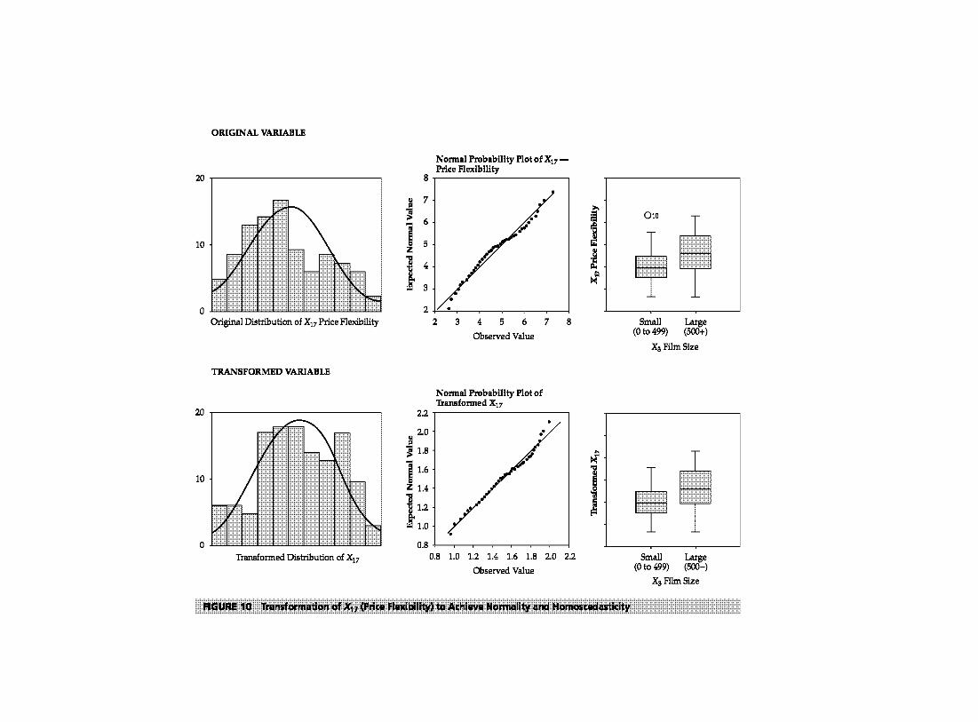
ORIGINAL VARIABLE

20 .-------------------------,

10

0-'----'---'---'-----'--"---'----'--'---'----''----' Original Distribution of X17 Price Flexibility

TRANSFORMED VARIABLE

20 .-------------------------,

10

0-'----'---'---'-----'--"---'----'--'---'----''----' Transformed Distribution of x17

Normal Probability Plot of X17 -Price Flexibility

8 .----------------------,

Cll 7 ::I

~ - 6

~ 5 :z:

l 4

~ 3

•• f'"

2 , •

2.2

2.0 ~ ~ 1.8

11.6 = :z: 1.4

1 1.2

!:\o

2 3 4 5 6 7

Observed Value

Normal Probability Plot of Transformed x17

.· ?

8

0.8 +----r---..-----.----,...---r-~r---l 0.8 1.0 1.2 1.4 1.6 1.8 2.0 2.2

Observed Value

~ :e ~ ~ ><~

" >< "0

J ~

FIGURE 10 Transformation of X17 (Price Flexibility) to Achieve Normality and Homoscedasticity

010

$ Small

(0 to 499) Large (500+)

X3 Fi!mSize

Small Large (0 to 499) (500+)

X3 FilmSize

Distribution Characteristics Before and After Transformation

SHAPE DESCRIPTORS Test of Normality

Skewness Kurtosis

Variable Form Statistic I z value• Statistic I z value• Statistic Significance

Original X17 .323 I 1.34 -.816 I -1.71 .1 01 .013

Transformed X17° -.121 I .50 -.803 I -1.68 .080 .117 "The z values are derived by dividing the statistics by the appropriate standard errors of .241 (skewness) and .478 (kurtosis). The equations for

calculating the standard errors are given in the text.

b Logarithmic transformation.

Levene Test Statistic

Xs x1 Xz X3 ~ Distribution

Variable Form Customer Type Industry Type Firm Size Region System

Original X17 5.56** 2.84 4.19* 16.21** .62

Transformed X17 2.76 2.23 1.20 3.11** .01

• Significant at .05 significance level.

•• Significant at .01 significance level.

FIGURE 10 Continued

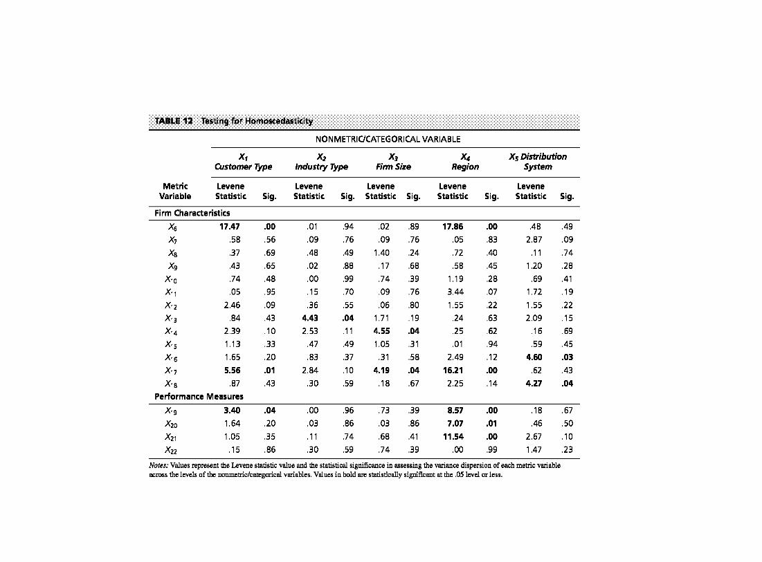
TABLE 12 Testing for Homoscedasticity

NONMETRIC/CATEGORICAL VARIABLE

x1 x2 X3 X4 X5 Distribution Customer Type Industry Type Firm Size Region System

Metric Levene Levene Levene Levene Levene Variable Statistic Sig. Statistic Sig. Statistic Sig. Statistic Sig. Statistic Sig.

Firm Characteristics

x6 17.47 .00 .01 .94 .02 .89 17.86 .00 .48 .49

X7 .58 .56 .09 .76 .09 .76 .05 .83 2.87 .09

X a .37 .69 .48 .49 1.40 .24 .72 .40 .11 .74

Xg .43 .65 .02 .88 .17 .68 .58 .45 1.20 .28

x,o .74 .48 .00 .99 .74 .39 1.19 .28 .69 .41

x,, .05 .95 .15 .70 .09 .76 3.44 .07 1.72 .19

x12 2.46 .09 .36 .55 .06 .80 1.55 .22 1.55 .22

x,3 .84 .43 4.43 .04 1. 71 .19 .24 .63 2.09 .15

x,4 2.39 .1 0 2.53 .11 4.55 .04 .25 .62 .16 .69

x,s 1.13 .33 .47 .49 1.05 .31 .01 .94 .59 .45

x,6 1.65 .20 .83 .37 .31 .58 2.49 .12 4.60 .03

x,7 5.56 .01 2.84 .1 0 4.19 .04 16.21 .00 .62 .43

x,s .87 .43 .30 .59 .18 .67 2.25 .14 4.27 .04

Performance Measures

X,g 3.40 .04 .00 .96 .73 .39 8.57 .00 .18 .67

X2o 1.64 .20 .03 .86 .03 .86 7.07 .01 .46 .50

X21 1.05 .35 .11 .74 .68 .41 11.54 .00 2.67 .1 0

X22 .15 .86 .30 .59 .74 .39 .00 .99 1.47 .23

Notes: Values represent the Levene statistic value and the statistical significance in assessing the variance dispersion of each metric variable across the levels of the non.metric/categorical variables. Values in bold are statistically significant at the .05 level or less.

Examining Your Data

LINEARITY The final assumption to be examined is the linearity of the relationships. In the case of individual variables, this linearity relates to the patterns of association between each pair of variables and the ability of the correlation coefficient to adequately represent the relationship. H nonlinear relationships are indicated, then the researcher can either transform one or both of the variables to achieve linearity or create additional variables to represent the nonlinear components. For our purposes, we rely on the visual inspection of the relationships to determine whether non­linear relationships are present. The reader can also refer to Figure 2, the scatterplot matrix containing the scatterplot for selected metric variables in the data set. Examination of the scatter­plots does not reveal any apparent nonlinear relationships. Review of the scatterplots not shown in Figure 2 also did not reveal any apparent nonlinear patterns. Thus, transformations are not deemed necessary. The assumption of linearity will also be checked for the entire multivariate model, as is done in the examination of residuals in multiple regression.

SUMMARY The series of graphical and statistical tests directed toward assessing the assumptions underlying the multivariate techniques revealed relatively little in terms of violations of the assump­tions. Where violations were indicated, they were relatively minor and should not present any seri­ous problems in the course of the data analysis. The researcher is encouraged always to perform these simple, yet revealing, examinations of the data to ensure that potential problems can be iden­tified and resolved before the analysis begins.

INCORPORATING NONMETRIC DATA WITH DUMMY VARIABLES

A critical factor in choosing and applying the correct multivariate technique is the measurement properties of the dependent and independent variables. Some of the techniques, such as discrimi­nant analysis or multivariate analysis of variance, specifically require nonmetric data as dependent or independent variables. In many instances, metric variables must be used as independent vari­ables, such as in regression analysis, discriminant analysis, and canonical correlation. Moreover, the interdependence techniques of factor and cluster analysis generally require metric variables. To this point, all discussions assumed metric measurement for variables. What can we do when the variables are nonmetric, with two or more categories? Are nonmetric variables, such as gender, marital status, or occupation, precluded from use in many multivariate techniques? The answer is no, and we now discuss how to incorporate nonmetric variables into many of these situations that require metric variables.

The researcher has available a method for using dichotomous variables, known as dummy variables, which act as replacement variables for the nonmetric variable. A dummy variable is a dichotomous variable that represents one category of a nonmetric independent variable. Any non­metric variable with k categories can be represented ask- 1 dummy variables. The following exam­ple will help clarify this concept.

First, assume we wish to include gender, which has two categories, female and male. We also have measured household income level by three categories (see Table 13). To represent the nonmetric variable gender, we would create two new dummy variables (X1 and X2), as shown in Table 13. X1 would represent those individuals who are female with a value of 1 and would give all males a value of 0. Likewise, X2 would represent all males with a value of 1 and give females a value of 0. Both variables (X1 and X~ are not necessary, however, because when X1 = 0, gender must be female by definition. Thus, we need include only one of the variables (X1 or X~ to test the effect of gender.

Correspondingly, if we had also measured household income with three levels, as shown in Table 13, we would first define three dummy variables (X3, X.. and X5). In the case of gender, we would not need the entire set of dummy variables, and instead use k- 1 dummy variables, where k

Examining Your Data

TABLE 13 Representing Nonmetric Variables with Dummy Variables

Nonmetric Variable with Two Categories (Gender)

Gender

Female

Male

Dummy Variables

X1 = 1, elseX1 = 0

X2 = 1, elseX2 = 0

Nonmetric Variable with Three Categories (Household Income Level)

Household Income Level

if <$15,000

if >$15,000 & ~$25,000 if>$25,000

Dummy Variables

X3 = 1, elseX3 = 0

x4 = 1, else x4 = 0 X5 = 1, elseX5 = 0

is the number of categories. Thus, we would use two of the dummy variables to represent the effects of household income.

In constructing dummy variables, two approaches can be used to represent the categories, and more importantly, the category that is omitted, known as the reference category or comparison group.

• The first approach is known as indicator coding, uses three ways to represent the household income levels with two dummy variables, as shown in Table 14. An important consideration is the reference category or comparison group, the category that received all zeros for the dummy variables. For example, in regression analysis, the regression coefficients for the dummy variables represent deviations from the comparison group on the dependent variable. The deviations represent the differences between the dependent variable mean score for each group of respondents (represented by a separate dummy variable) and the comparison group. This form is most appropriate in a logical comparison group, such as in an experiment In an experiment with a control group acting as the comparison group, the coefficients are the mean differences on the dependent variable for each treatment group from the control group. Any time dummy variable coding is used, we must be aware of the comparison group and remem­ber the impacts it has in our interpretation of the remaining variables.

• An alternative method of dummy variable coding is termed effects coding. It is the same as indicator coding except that the comparison group (the group that got all zeros in indicator coding) is now given the value of -1 instead of 0 for the dummy variables. Now the coeffi­cients represent differences for any group from the mean of all groups rather than from the omitted group. Both forms of dummy variable coding will give the same results; the only dif­ferences will be in the interpretation of the dummy variable coefficients.

Dummy variables are used most often in regression and discriminant analysis, where the coef­ficients have direct interpretation. Their use in other multivariate techniques is more limited, espe­cially for those that rely on correlation patterns, such as factor analysis, because the correlation of a binary variable is not well represented by the traditional Pearson correlation coefficient. However, special considerations can be made in these instances.

TABLE 14 Alternative Dummy Variable Coding Patterns for a Three-category Nonmetric Variable

Pattern 7 Pattern2 Pattern3

Household Income Level x, x2 x, x2 x, x2 If <$15,000 1 0 1 0 0 0 If >$15,000 & ~$25,000 0 1 0 0 1 0 If >$25,000 0 0 0 1 0 1

Examining Your Data

Summary Researchers should examine and explore the nature of the data and the relationships among variables before the application of any of the multivariate techniques. This chapter helps the researcher to do the following:

Select the appropriate graphical method to examine the characteristics of the data or relationships of interest. Use of multivariate techniques places an increased bunJen on the researcher to understand, evaluate, and interpret the more complex results. It requires a thor­ough understanding of the basic characteristics of the underlying data and relationships. The first task in data examination is to determine the character of the data. A simple, yet powerful, approach is through graphical dis­plays, which can portray the univariate, bivariate, and even multivariate qualities of the data in a visual format for ease of display and analysis. The starting point for understand­ing the nature of a single variable is to characterize the shape of its distribution, which is accomplished with a his­togram. The most popular method for examining bivariate relationships is the scatterplot, a graph of data points based on two variables. Researchers also should examine multi­variate profiles. Three types of graphs are used. The first graph type is a direct portrayal of the data values, either by glyphs that display data in circles or multivariate profiles that provide a barlike profile for each observation. A second type of multivariate display involves a transformation of the original data into a mathematical relationship, which can then be portrayed graphically. The most common technique of this type is the Fourier transformation. The third graphi­cal approach is iconic representativeness, the most popular being the Chernoff face.

Assess the type and potential impact of missing data. Although some missing data can be ignored, missing data is still one of the most troublesome issues in most research settings. At its best, it is a nuisance that must be remedied to allow for as much of the sample to be analyzed as possible. In more problematic situations, however, it can cause serious biases in the results if not correctly identified and accommodated in the analysis. The four-step process for identifying missing data and applying remedies is as follows:

1. Determine the type of missing data and whether or not it can be ignored.

2. Determine the extent of missing data and decide whether respondents or variables should be deleted.

3. Diagnose the randomness of the missing data. 4. Select the imputation method for estimating missing

data.

Understand the different types of missing data processes. A missing data process is the underlying cause for missing data, whether it be something involv­ing the data collection process (poorly worded ques­tions, etc.) or the individual (reluctance or inability to answer, etc.). When missing data are not ignorable, the missing data process can be classified into one of two types. The first is MCAR, which denotes that the effects of the missing data process are randomly dis­tributed in the results and can be remedied without incurring bias. The second is MAR, which denotes that the underlying process results in a bias (e.g., lower response by a certain type of consumer) and any rem­edy must be sure to not only "fix" the missing data, but not incur bias in the process.

Explain the advantages and disadvantages of the approaches available for dealing with missing data. The remedies for missing data can follow one of two approaches: using only valid data or cal­culating replacement data for the missing data. Even though using only valid data seems a reasonable approach, the researcher must remember that doing so assures the full effect of any biases due to non­random (MAR) data processes. Therefore, such approaches can be used only when random (MCAR) data processes are present, and then only if the sam­ple is not too depleted for the analysis in question (remember, missing data excludes a case from use in the analysis). The calculation of replacement values attempts to impute a value for each missing value, based on criteria ranging from the sample's overall mean score for that variable to specific characteris­tics of the case used in a predictive relationship. Again, the researcher must first consider whether the effects are MCAR or MAR, and then select a remedy balancing the specificity of the remedy ver­sus the extent of the missing data and its effect on generalizability.

Identify univariate, bivariate, and multivariate outliers. Outliers are observations with a unique com­bination of characteristics indicating they are distinctly different from the other observations. These differences can be on a single variable (univariate outlier), a relation­ship between two variables (bivariate outlier), or across an entire set of variables (multivariate outlier). Although the causes for outliers are varied, the primary issue to be resolved is their representativeness and whether the observation or variable should be deleted or included in the sample to be analyzed.

Examining Your Data

Test your data for the assumptions underlying most multivariate techniques. Because our analyses involve the use of a sample and not the population, we must be concerned with meeting the assumptions of the statistical inference process that is the foundation for all multivariate statistical techniques. The most important assumptions include normality, homoscedasticity, lin­earity, and absence of correlated errors. A wide range of tests, from graphical portrayals to empirical measures, is available to determine whether assumptions are met. Researchers are faced with what may seem to be an impossible task: satisfy all of these statistical assump­tions or risk a biased and flawed analysis. These statisti­cal assumptions are important, but judgment must be used in how to interpret the tests for each assumption and when to apply remedies. Even analyses with small sample sizes can withstand small, but significant, depar­tures from normality. What is more important for the researcher is to understand the implications of each assumption with regard to the technique of interest, striking a balance between the need to satisfy the assumptions versus the robustness of the technique and research context.

Determine the best method of data transformation given a specific problem. When the statistical assump­tions are not met, it is not necessarily a ''fatal" problem that prevents further analysis. Instead, the researcher may be able to apply any number of transformations to the data in question that will solve the problem and enable the assumptions to be met. Data transformations provide a means of modifying variables for one of two reasons: (1) to correct violations of the statistical assumptions

Questions 1. Explain how graphical methods can complement the empir­

ical measures when examining data. 2. List potential underlying causes of outliers. Be sure to include

attributions to both the respondent and the researcher. 3. Discuss why outliers might be classified as beneficial and

as problematic. 4. Distinguish between data that are missing at random

(MAR) and missing completely at random (MCAR). Explain how each type affects the analysis of missing data.

Suggested Readings

underlying the multivariate techniques, or (2) to improve the relationship (correlation) between variables. Most of the transformations involve modifying one or more vari­ables (e.g., compute the square root, logarithm, or inverse) and then using the transformed value in the analysis. It should be noted that the underlying data are still intact, just their distributional character is changed so as to meet the necessary statistical assumptions.

Understand how to incorporate nonmetric variables as metric variables. An important consideration in choosing and applying the correct multivariate technique is the measurement properties of the dependent and independent variables. Some of the techniques, such as discriminant analysis or multivariate analysis of vari­ance, specifically require nonmetric data as dependent or independent variables. In many instances, the multivari­ate methods require that metric variables be used. Yet nonmetric variables are often of considerable interest to the researcher in a particular analysis. A method is avail­able to represent a nonmetric variable with a set of dichotomous variables, known as dummy variables, so that it may be included in many of the analyses requiring only metric variables. A dummy variable is a dichoto­mous variable that has been converted to a metric distri­bution and represents one category of a nonmetric independent variable.

Considerable time and effort can be expended in these activities, but the prudent researcher wisely invests the necessary resources to thoroughly examine the data to ensure that the multivariate methods are applied in appro­priate situations and to assist in a more thorough and insightful intetpretation of the results.

5. Describe the conditions under which a researcher would delete a case with missing data versus the conditions under which a researcher would use an imputation method.

6. Evaluate the following statement: In order to run most mul­tivariate analyses, it is not necessary to meet all the assump­tions of normality, linearity, homoscedasticity, and independence.

7. Discuss the following statement: Multivariate analyses can be run on any data set, as long as the sample size is adequate.

A list of suggested readings illustrating the issues in examining data in specific applications is available on the Web at www.pearsonhighered.com/hair or www.mvstats.com.

Examining Your Data

References 1. Anderson, Edgar. 1969. A Semigraphical Method for the

Analysis of Complex Problems. Technometrics 2 (August): 387-91.

2. Arbuckle, J. 1996. Full Information Estimation in the Presence of Incomplete Data. In Advanced Structural Equation Modeling: Issues and Techniques, G. A. Marcoulides and R. E. Schumacher (eds.). Mahwah, NJ: LEA.

3. Box, G. E. P., and D. R. Cox. 1964. An Analysis of Transformations. Journal of the Royal Statistical Society B 26: 211--43.

4. Brown, R. L. 1994. Efficacy of the Indirect Approach for Estimating Structural Equation Models with Missing Data: A Comparison of Five Methods. Structural Equation Modeling 1: 287-316.

5. Chernoff, Herman. 1978. Graphical Representation as a Discipline. In Graphical Representation of Multivariate Data, Peter C. C. Wang (ed.). New York: Academic Press, pp. 1-11.

6. Cohen, Jacob, Stephen G. West, Leona Aiken, and Patricia Cohen. 2002. Applied Multiple Regression/Correlation Analysis for the Behavioral Sciences, 3rd ed. Hillsdale, NJ: Lawrence Erlbaum Associates.

7. Daniel, C., and F. S. Wood. 1999. Fitting Equations to Data, 2nd ed. New York: Wiley-Interscience.

8. Dempster, A. P., and D. B. Rubin. 1983. Overview. In Incomplete Data in Sample Surveys: Theory and Annotated Bibliography, Vol. 2., Madow, Olkin, and Rubin (eds.). New York: Academic Press.

9. Duncan, T. E., R. Omen, and S. C. Duncan. 1994. Modeling Incomplete Data in Exercise Behavior Using Structural Equation Methodology. Journal of Sport and Exercise Psychology 16: 187-205.

10. Feinberg, Stephen. 1979. Graphical Methods in Statistics. American Statistician 33 (November): 165-78.

11. Graham, J. W., and S. W. Donaldson. 1993. Evaluating Interventions with Differential Attrition: The Importance of Nonresponse Mechanisms and Use of Follow-up Data. Journal of Applied Psychology 78: 119-28.

12. Graham, J. W., S. M. Hofer, and D. P. MacKinnon. 1996. Maximizing the Usefulness of Data Obtained with Planned

Missing Value Patterns: An Application of Maximum Likelihood Procedures. Multivariate Behavioral Research 31(2): 197-218.

13. Gnanedesikan, R. 1977. Methods for Statistical Analysis of Multivariate Distributions. New York: Wiley.

14. Heitjan, D. F. 1997. Annotation: What Can Be Done About Missing Data? Approaches to Imputation. American Journal of Public Health 87(4): 548--50.

15. Hertel, B. R. 1976. Minimizing Error Variance Introduced by Missing Data Routines in Survey Analysis. Sociological Methods and Research 4: 459-74.

16. Johnson, R. A., and D. W. Wichern. 2002. Applied Multivariate Statistical Analysis. 5th ed. Upper Saddle River, NJ: Prentice Hall.

17. Kim, J. 0., and J. Curry. 1977. The Treatment of Missing Data in Multivariate Analysis. Sociological Methods and Research 6: 215--41.

18. Little, Roderick J. A., and Donald B. Rubin. 2002. Statistical Analysis with Missing Data. 2nd ed. New York: Wiley.

19. Malhotra, N. K. 1987. Analyzing Marketing Research Data with Incomplete Information on the Dependent Variables. Journal of Marketing Research 24: 74--84.

20. Raymonds, M. R., and D. M. Roberts. 1987. A Comparison of Methods for Treating Incomplete Data in Selection Research. Educational and Psychological Measurement 47: 13--26.

21. Roth, P. L. 1994. Missing Data: A Conceptual Review for Applied Psychologists. Personnel Psychology 47: 537--60.

22. Schafer, J. L. 1997. Analysis of Incomplete Multivariate Data. London: Chapman and Hall.

23. Stevens, J. 2001. Applied Multivariate Statistics for the Social Sciences, 4th ed. Hillsdale, NJ: Lawrence Erlbaum Publishing.

24. Wang, Peter C. C. (ed.). 1978. Graphical Representation of Multivariate Data. New York: Academic Press.

25. Weisberg, S. 1985. Applied Linear Regression. New York: Wiley.

26. Wilkinson, L. 1982. An Experimental Evaluation of Multivariate Graphical Point Representations. In Human Factors in Computer Systems: Proceedings. New York: ACM Press, pp. 202-9.