Examination of polarization coupling in a plucked musical instrumentstring via experiments and simulationsAlexander Brauchler, Pascal Ziegler, and Peter Eberhard*

Institute of Engineering and Computational Mechanics, University Stuttgart, Pfaffenwaldring 9, 70569 Stuttgart, Germany

Received 2 April 2020, Accepted 4 June 2020

Abstract – In this article, the transient motion of a realistically plucked guitar string is studied experimentallyand numerically in both transversal polarizations. The frequency dependent damping and suitable initial con-ditions are identified in the experiment and used in a simulation. For this reason an experimental set-up con-sisting of a string, an excitation mechanism and two laser Doppler vibrometers is developed. The excitationmechanism performs a realistic and reproducible plucking motion with a plectrum. Two laser Doppler vibrom-eters are used to measure the string oscillation transversally in two polarizations. The experimental set-upmakes it possible to measure the string’s motion under reproducible conditions and, hence, at different positionsfor the same oscillation. This capability renders the identification of suitable initial conditions, i.e., initial dis-placement and velocity as well as the pre-tension, for a string model possible. Furthermore, a finite elementmodel for the string is developed that takes into account the oscillation in both transversal planes of polariza-tion and the coupling between them. Finally, the model results are in good agreement with the measurements.With help of the numerical model it can be vividly shown that the coupling between the polarizations of theoscillation is due to a torsional movement of the string on the saddle.

Keywords: Guitar string vibration, Musical instruments, Realistic plucking, LDV measurement,Experimental study, Numerical study

1 Introduction

The acoustic guitar is a popular string instrument inwhich the sound results from a mechanical process begin-ning with the oscillation of the plucked string. The soundof the string is influenced by several physical effects like dis-persion and damping which are difficult to describe andconsider. Dispersion results from the bending stiffness ofthe string and shifts the overtones to relatively higher fre-quencies. Moreover, the frequency dependent damping ofthe string influences the oscillation to a large extend [1].

The basic mathematical model for a vibrating string isthe one-dimensional wave equation which can be found inmany textbooks. Usually, this is extended by additionalterms to include physical effects like damping or dispersion[2–4]. A comparison of different stiff string models can befound in Ducceschi and Bilbao [5]. Besides finite differencesimulations of these stiff string models [6, 7] digital wave-guide models are a common approach [8, 9].

Specifically for the guitar, the work of Woodhouse is tomention [1, 10]. In these publications three numericalmodels, namely frequency-domain, time-domain and modalsuperposition methods, for the acoustic guitar are compared

to each other and to experiments. However, the results com-pared to the experiment were not satisfying for a transientmeasurement of the string oscillation.

Recent sophisticated string models contain the afore-mentioned physical features and show very realistic resultswhen compared to experiments. For example one study isengaged in piano modeling and is using a Timoshenko beammodel which shows a good result for the string motionwhen compared to an experiment [11]. The piano stringsare struck and not plucked and only one transversalpolarization of the string oscillation is excited and includedin the model. Furthermore, contacts with the fretboard ofa guitar are included in models and the simulation resultsare shown to be in very good agreement with experiments[12, 13]. However, to make a comparison with an experi-mental measurement possible, the string was excited usinga copper wire in those studies. This method produces simpleinitial conditions for a numerical model but they are notrealistic.

Moreover, many publications exist on the purely experi-mental measurement of the string oscillation. The methodsto measure the oscillation include the electromagneticpickup [14], an electrodynamic method [15], or electric field

*Corresponding author: peter.eberhard@itm.uni-stuttgart.de

This is an Open Access article distributed under the terms of the Creative Commons Attribution License (https://creativecommons.org/licenses/by/4.0),which permits unrestricted use, distribution, and reproduction in any medium, provided the original work is properly cited.

Acta Acustica 2020, 4, 9

Available online at:

�A. Brauchler et al., Published by EDP Sciences, 2020

https://acta-acustica.edpsciences.org

https://doi.org/10.1051/aacus/2020008

SCIENTIFIC ARTICLE

sensing methods [16] which are applicable to a steel stringonly. In other publications optical measurement techniqueslike opto-switch sensors [17], high-speed cameras [18], orlaser Doppler vibrometers (LDVs) [19] are used. On theother hand, publications are not only concerned with thestring oscillation but also with the player and the pluckingmotion which has a great influence on the instrumentssound. There have been studies about the plucking actioninvestigating the motion of the plectrum and the string ina harpsichord for different plectrum shapes and pluckingstrengths [20, 21]. Another study is concerned about theplucking of a harp [22]. Nevertheless, these studies areessentially experimental and do not include a numericalmodel for the string oscillation after the excitation.

Previous studies found two eigenfrequencies very closeto each other for the string oscillation close to the bridgeof an instrument [1]. This effect can be explained by thetwo polarization planes of the string’s oscillation havingslightly different effective lengths and, hence, differenteigenfrequencies. In Bank and Karjalainen [23] it is stated,that the guitar bridge acts as a mechanical coupling devicefor the two planes of polarization in the string oscillationand causes this effect.

The aim and novel contribution of this study is, to com-bine the previous findings with a realistically plucked stringin a reproducible experiment and a well suited numericalmodel to approximate the plucked string motion in bothtransversal polarizations. Furthermore, the coupling of thetwo transversal polarizations through a plain half-roundsaddle is examined. To reach this goal, damping parametersand complex initial conditions for the numerical modelmust be identified from an experiment for one particularstring. Therefore, an experimental set-up with an excitationmechanism that yields a reproducible and realistic pluckingmotion is developed. The results of the numerical model arecompared with the experimental results of the realisticallyplucked string. The novel contribution is not only themethod to identify the initial conditions for the entire stringusing a most realistic, reproducible excitation and theirapplication to the numerical string model, but also theexamination of the polarization coupling in a very vividway through the numerical model. Finally, this procedureresults in a very good agreement of numerical simulationand experimental measurement.

2 Experimental study

The sound of an acoustic guitar results from an interac-tion between the guitar body and the string through thebridge. In this work the string shall be examined withoutany influence from the guitar body. This is why a singlestring is mounted on guitar-like saddles without a body.The experiment is carried out firstly to reproducibly mea-sure the oscillation of the string under realistic pluckingconditions. Secondly, the frequency dependent dampingratio shall be identified, and thirdly, the coupling of thetwo polarizations of the string is examined. Furthermore,suitable initial conditions for a simulation are identified.

2.1 Experimental set-up

In the center of the experiment is a bare steel string ofan electrical guitar set (Harley Benton Valuestrings 010)with diameter d = 0.43 mm (third string), which is high-lighted in blue in Figure 1. It is clamped between two equalbrass saddles assembled in a guitar typical distance ofL = 0.65 m. The string can be tuned to the desired tensionwith a machine head from a guitar. The measurement iscarried out with two LDVs of type Polytec OFV 303. Oneof them measures velocity and displacement of the stringat a certain position in horizontal direction while the otherone measures the vertical displacement and velocity at thesame position. The LDVs allow an accurate measurementof even very small displacements of the string in bothtransversal polarizations.

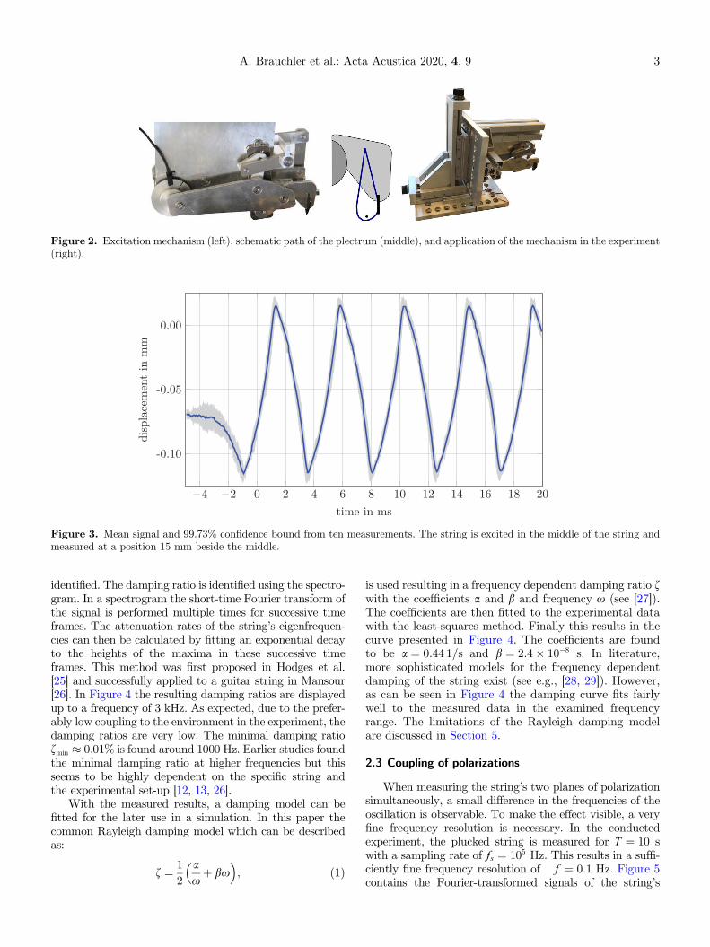
Another central part of the experimental set-up is theexcitation mechanism displayed in Figure 2. The mechan-ism was built to replicate a human-like plucking of thestring with a plectrum [24]. For the experiments throughoutthis paper a thin standard plectrum with thicknessdpl = 0.46 mm is used. The motor driven mechanism con-sists of five parts transforming the circular motion into arealistic plucking movement. Furthermore, the mechanismyields reproducibility in intensity, point of action anddirection of the motion [24]. To realize a fine adjustableplucking position and strength the mechanism is mountedon a horizontally and vertically movable mechanical adjus-ter. Figure 3 shows the mean value and the uncertainty often measured displacement signals of the vertical LDV. Itis clearly visible that the excitation mechanism produceswell-reproducible signals. Reproducible excitation yieldsthe advantage that the string can be excited multiple timesat the same position while the measurement can be carriedout at different positions.

2.2 Identification of damping

Besides measuring the string oscillation at differentpositions, the frequency dependent damping ratio shall be

Figure 1. Experimental set-up of the string with two LDVs andautomatic excitation mechanism.

A. Brauchler et al.: Acta Acustica 2020, 4, 92

identified. The damping ratio is identified using the spectro-gram. In a spectrogram the short-time Fourier transform ofthe signal is performed multiple times for successive timeframes. The attenuation rates of the string’s eigenfrequen-cies can then be calculated by fitting an exponential decayto the heights of the maxima in these successive timeframes. This method was first proposed in Hodges et al.[25] and successfully applied to a guitar string in Mansour[26]. In Figure 4 the resulting damping ratios are displayedup to a frequency of 3 kHz. As expected, due to the prefer-ably low coupling to the environment in the experiment, thedamping ratios are very low. The minimal damping ratiofmin � 0.01% is found around 1000 Hz. Earlier studies foundthe minimal damping ratio at higher frequencies but thisseems to be highly dependent on the specific string andthe experimental set-up [12, 13, 26].

With the measured results, a damping model can befitted for the later use in a simulation. In this paper thecommon Rayleigh damping model which can be describedas:

f ¼ 12

axþ bx

� �; ð1Þ

is used resulting in a frequency dependent damping ratio fwith the coefficients a and b and frequency x (see [27]).The coefficients are then fitted to the experimental datawith the least-squares method. Finally this results in thecurve presented in Figure 4. The coefficients are foundto be a ¼ 0:44 1=s and b ¼ 2:4� 10�8 s. In literature,more sophisticated models for the frequency dependentdamping of the string exist (see e.g., [28, 29]). However,as can be seen in Figure 4 the damping curve fits fairlywell to the measured data in the examined frequencyrange. The limitations of the Rayleigh damping modelare discussed in Section 5.

2.3 Coupling of polarizations

When measuring the string’s two planes of polarizationsimultaneously, a small difference in the frequencies of theoscillation is observable. To make the effect visible, a veryfine frequency resolution is necessary. In the conductedexperiment, the plucked string is measured for T ¼ 10 swith a sampling rate of fs ¼ 105 Hz. This results in a suffi-ciently fine frequency resolution of �f ¼ 0:1 Hz. Figure 5contains the Fourier-transformed signals of the string’s

Figure 2. Excitation mechanism (left), schematic path of the plectrum (middle), and application of the mechanism in the experiment(right).

Figure 3. Mean signal and 99.73% confidence bound from ten measurements. The string is excited in the middle of the string andmeasured at a position 15 mm beside the middle.

A. Brauchler et al.: Acta Acustica 2020, 4, 9 3

velocity in horizontal and vertical polarization. Besides theexpected similarity in the upper plot, it is clearly visible inthe lower plot that the frequencies of the two planes ofpolarization deviate from each other by about 0.2 Hz atthe first eigenfrequency.

Another effect is visible when the orbit diagram display-ing the vertical oscillation over the horizontal oscillation isexamined. Figure 6 shows the transient development of theorbit diagram via four cycles of the oscillation within thefirst second of free oscillation. Together with a dampingeffect it is clearly visible that the shape of the orbit varieswith time. The shape variation can be explained by disper-sion and the small frequency difference between the twoplanes of polarization.

In literature, multiple possible causes for the frequencydifference are found. Firstly, nonlinear behavior due to large

amplitudes might couple the polarizations and add furtherfrequencies to the spectrum [26, 30]. Secondly, the saddlemight influence the strings oscillation due to coupling ofthe saddle’s vibration with the string’s vibration [30].Furthermore, a stick-slip movement owing to friction or atorsional movement of the string of the string on the saddlemight cause the observed effect [1, 26].

In all presented measurements the amplitudes of thestring oscillation are always smaller than the string’s dia-meter and, therefore, nonlinear effects are very small.Although nonlinear effects like phantom partials cannotbe ruled out completely for higher overtones they are veryunlikely to cause the observed effect. Moreover, as exam-ined in literature, there is influence of large displacementon the orbit of the string but displacements would haveto be larger by at least one order of magnitude to see that

Figure 4. Identified damping ratios over frequency for several experiments and fitted Rayleigh damping curve.

Figure 5. Fourier transformed velocity signal in the two planes of polarization.

A. Brauchler et al.: Acta Acustica 2020, 4, 94

influence [30]. Consequently, nonlinear effects are insignifi-cant and can be ruled out as the cause for the observedbehavior. If a complete guitar was examined, it would beevident that the oscillation of the bridge influences the oscil-lation of the string. However, in the presented experimentthe saddles are very rigid compared to the string and addi-tional experiments showed clearly that the amplitude of thesaddle’s vibration is at least two orders of magnitudesmaller than the amplitude of the vibration of the string.So in the further numerical investigation, the vibration ofthe saddles is neglected.

Hence, only stick-slip friction and torsion of the stringremain as possible causes for the frequency deviationbetween the polarizations. Both effects would influence thefrequency mainly in horizontal direction due to horizontalmovement on the saddle. Yet, preliminary simulationssuggested that a string slipping over the saddle causes adifferent damping behavior than the one observed in theexperiments. As the string underwent a slipping movementon the saddle, a high damping in the beginning of the oscil-lation occured and after a small number of cycles the stringwould stick on the saddle. Therefore, for a stick-slip move-ment a decaying frequency difference between the twoplanes of polarization was observed. On the contrary, themeasured string oscillation shows a constant frequencydifference and very small damping for a long measurement(T ¼ 10 s) from the beginning until the end. Consideringthis, the research hypothesis that a torsional movement ofthe string on the saddle, rather than slipping, causes thefrequency difference between the two planes of polarizationis concluded. In the following, a numerical model is proposedthat is capable of showing vividly that a torsional movement

of the string, in fact, causes this behavior while excluding allother possible influences and, hence, this confirms theresearch hypothesis.

3 Numerical model

A realistic string model should include physical effectslike damping and dispersion as well as both transversalpolarizations of the string oscillation and the couplingbetween them. Dispersion describes the frequency depen-dent wave velocity due to bending stiffness of the stringleading to slightly higher overtones in reality than the idealharmonic overtones [2]. The classical wave equation whichdates back to D’Alembert does not cover these phenomena.Furthermore, most publications are only modeling a one-dimensional string oscillation, but the experimental resultsdescribed in Section 4 make clear that both transversalpolarizations are necessary for a model of a realisticallyplucked string. Here, a finite element (FE) model of thestring is developed using mainly Euler-Bernoulli beamelements in the commercial software Abaqus [31].

3.1 Mechanical model

In the following, the FE model is described taking notonly physical effects like geometrical stiffness and dispersioninto account, but also both planes of polarization and thecoupling between them. To include the effect of torsionalmovement of the string on the saddle, the string model con-sists of three parts as can be seen in Figure 7. As the string isplucked in the middle, symmetry is used and a half model iscreated which consists of the main part of the string and atailpiece discretized with beam elements of type AbaqusB31. In these elements, the Euler–Bernoulli beam model isused which has proven to be a good model for bare steelguitar strings [5, 12]. A Timoshenko beam model wouldbe another option and was investigated by the authors butis avoided here due to numerical issues that might ariseand because the Timoshenko model only has physicaladvantages for thicker strings as for example used in a piano[5, 32].

The distribution of eigenfrequencies of a string is depen-dent on the tension. This stiffening effect due to tension isincluded in Abaqus when using geometric nonlinearities.Then, also nonlinear effects owing to large displacementsare included automatically. As a steel string is used in theexperiment, typical material properties for steel are usedin the model with Young’s modulus E ¼ 210 GPa, Poissonratio m ¼ 0:3 and density q ¼ 7900 kg=m3. During thedynamic simulation a Hilber–Hughes–Taylor implicit timeintegrator is used with a maximum time step of�t ¼ 10�5 s [31].

The dimension of the main string and the tailpiece aredirectly taken from the measured string. This results in alength lmain ¼ 325 mm of the main part and the lengthltail ¼ 55 mm for the tailpiece. A round cross section withthe string’s diameter d ¼ 0:43 mm is assumed. Both partsof the string are sufficiently fine meshed by 128 elements

Figure 6. Transient development of the measured orbitdiagram at four points in time close to the middle of the string.

A. Brauchler et al.: Acta Acustica 2020, 4, 9 5

in the half string and 100 elements in the tailpiece.Although the cross section of the string is included in themathematical model through the moment of inertia, andtorsional stress can be calculated, geometrically the dia-meter of the beam model is zero. Thus, it is not possible todescribe a string performing a torsional motion with thesebeam elements. This is why a small third section describingthe part of the string which is in contact with the saddle ismodeled and discretized with volume elements of type Aba-qus C3D8R. The volume elements yield the advantage thatthey discretize a three dimensional continuum and, hence,this three dimensional continuum can perform a rotationalmovement instead of just calculating torsional stress as isdone in the beam elements. Of course it would be possibleto discretize the whole string with volume elements but justthe small section of length lvol ¼ 1 mm must already be dis-cretized with 10 160 elements. The three parts of the stringmodel are connected via kinematic constraints binding thetwo lateral degrees of freedom of the adjacent node of thebeam element section to the area of the volume elementsection. Figure 7 shows a schematical visualization of themodel with an exaggerated volume part. The boundaryconditions at the end of the tailpiece, the right end (middle)of the string and the artificial contact boundary conditionare displayed as well in the figure.

On that contact piece discretized with volume elementsa small area is defined as contact area with the saddle con-sisting of only six nodes. In this small area the two transla-tional degrees of freedom orthogonal to the string axis areconstrained. For a small rotation, this boundary conditionis similar to the string sticking on the saddle. At the endof the tailpiece, which is bended in the same angle ofu = 15� as in the experiment, all degrees of freedom are con-strained. It is needless to say that this model comes acrossquite artificially but with this model it is certainly possibleto isolate the effect of a torsional movement of the string onthe saddle which might cause the frequency difference and,hence, the specific development of the orbit plot discussedin Section 2.3.

3.2 Simulation procedure

The goal of the simulation is to reproduce the stringoscillation after the excitation. Therefore, suited initialconditions consisting of an initial displacement and aninitial velocity as well as a pre-tension have to be appliedto the model [22]. In Abaqus it is not possible to apply theinitial conditions and the pre-tension directly in the samecomputation step. This is why three pre-simulation stepsare carried out.

To begin with, the tension is not applied directly but viaa longitudinal force on the model that results in a tension.This force can be well approximated by:

F L ¼ qp LDf 0ð Þ2; ð2Þwhere the length L, the diameter D, the density q and thefundamental frequency f0 are easy to measure from theexperiment [14]. In the simulation the fixed longitudinalboundary condition is removed at the end of the tailpieceand the longitudinal force is applied there. The force isapplied with the angle u = 15� to reach the desired tail-piece angle matching the one in the experiment. A staticsimulation step is carried out to find the new equilibrium.When the step is finished, the displacements are stored andall degrees of freedom at the supported node are restrainedsuch that the string cannot move longitudinally anymore.

After the first simulation step is carried out, the initialdisplacement cannot be directly imposed on the nodes ofthe model anymore. This is why a transversal force isapplied on the model in a second static simulation step atthe excited node such that the required displacement ofthe string is obtained. In this case, direction and magnitudeof the force are approximated from the results of the experi-ment. Furthermore, the initial velocity field at the timeinstant when the free oscillation of the string begins, isobtained. This velocity field identified in Section 4 isapplied directly to each node in a subsequent dynamic time-step. After finishing these three pre-simulation steps theactual free oscillation of the string can be simulated.

4 Experimental identification of initialconditions

Next, the plucking procedure is examined to identifysuitable initial conditions. The main issue here is, findingthe time instance where the contact between plectrumand string ends and the free oscillation begins. As a startingpoint the orbit diagram at a position very close to theexcited position displayed in Figure 8 is regarded. In thisstudy the string is plucked in the middle. Measuring exactlyat the plucking position is technically not feasible becausethe excitation mechanism does not leave room for the laserrays. However, the string’s behavior at a position very closeto the plucking position is assumed to be very similar tothat exactly at the plucking point.

The movement of the string during the plucking proce-dure can be divided into four phases as highlighted inFigure 8. In the beginning, the string sticks to the plectrum(phase 1). After the sticking phase the string and the plec-trum show alternately sticking and slipping behavior (phase2). In the third phase the string detaches from the plectrumand finally starts the free oscillation in the fourth phase.In the beginning the string undergoes a slow, nearly hori-zontal movement indicating that the string is moving withthe plectrum. Here the plectrum is only slightly bent. Afterthis phase in which the string sticks to the plectrum, stick-ing and slipping are alternating as the plectrum is further

Figure 7. Schematical visualization of the half-string FE modelincluding the coupling between beam and volume elements.

A. Brauchler et al.: Acta Acustica 2020, 4, 96

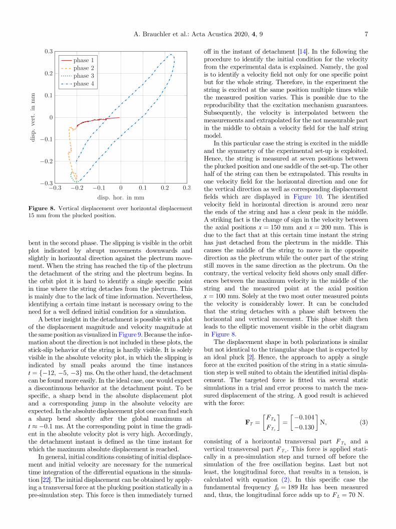
bent in the second phase. The slipping is visible in the orbitplot indicated by abrupt movements downwards andslightly in horizontal direction against the plectrum move-ment. When the string has reached the tip of the plectrumthe detachment of the string and the plectrum begins. Inthe orbit plot it is hard to identify a single specific pointin time where the string detaches from the plectrum. Thisis mainly due to the lack of time information. Nevertheless,identifying a certain time instant is necessary owing to theneed for a well defined initial condition for a simulation.

A better insight in the detachment is possible with a plotof the displacement magnitude and velocity magnitude atthe same position as visualized in Figure 9. Because the infor-mation about the direction is not included in these plots, thestick-slip behavior of the string is hardly visible. It is solelyvisible in the absolute velocity plot, in which the slipping isindicated by small peaks around the time instancest ¼ �12; �5; �3f g ms. On the other hand, the detachmentcan be found more easily. In the ideal case, one would expecta discontinuous behavior at the detachment point. To bespecific, a sharp bend in the absolute displacement plotand a corresponding jump in the absolute velocity areexpected. In the absolute displacement plot one canfind sucha sharp bend shortly after the global maximum att � �0:1 ms. At the corresponding point in time the gradi-ent in the absolute velocity plot is very high. Accordingly,the detachment instant is defined as the time instant forwhich the maximum absolute displacement is reached.

In general, initial conditions consisting of initial displace-ment and initial velocity are necessary for the numericaltime integration of the differential equations in the simula-tion [22]. The initial displacement can be obtained by apply-ing a transversal force at the plucking position statically in apre-simulation step. This force is then immediately turned

off in the instant of detachment [14]. In the following theprocedure to identify the initial condition for the velocityfrom the experimental data is explained. Namely, the goalis to identify a velocity field not only for one specific pointbut for the whole string. Therefore, in the experiment thestring is excited at the same position multiple times whilethe measured position varies. This is possible due to thereproducibility that the excitation mechanism guarantees.Subsequently, the velocity is interpolated between themeasurements and extrapolated for the not measurable partin the middle to obtain a velocity field for the half stringmodel.

In this particular case the string is excited in the middleand the symmetry of the experimental set-up is exploited.Hence, the string is measured at seven positions betweenthe plucked position and one saddle of the set-up. The otherhalf of the string can then be extrapolated. This results inone velocity field for the horizontal direction and one forthe vertical direction as well as corresponding displacementfields which are displayed in Figure 10. The identifiedvelocity field in horizontal direction is around zero nearthe ends of the string and has a clear peak in the middle.A striking fact is the change of sign in the velocity betweenthe axial positions x ¼ 150 mm and x ¼ 200 mm. This isdue to the fact that at this certain time instant the stringhas just detached from the plectrum in the middle. Thiscauses the middle of the string to move in the oppositedirection as the plectrum while the outer part of the stringstill moves in the same direction as the plectrum. On thecontrary, the vertical velocity field shows only small differ-ences between the maximum velocity in the middle of thestring and the measured point at the axial positionx ¼ 100 mm. Solely at the two most outer measured pointsthe velocity is considerably lower. It can be concludedthat the string detaches with a phase shift between thehorizontal and vertical movement. This phase shift thenleads to the elliptic movement visible in the orbit diagramin Figure 8.

The displacement shape in both polarizations is similarbut not identical to the triangular shape that is expected byan ideal pluck [2]. Hence, the approach to apply a singleforce at the excited position of the string in a static simula-tion step is well suited to obtain the identified initial displa-cement. The targeted force is fitted via several staticsimulations in a trial and error process to match the mea-sured displacement of the string. A good result is achievedwith the force:

FT ¼ F Th

F T v

� �¼ �0:104

�0:130

� �N; ð3Þ

consisting of a horizontal transversal part FTh and avertical transversal part FTv . This force is applied stati-cally in a pre-simulation step and turned off before thesimulation of the free oscillation begins. Last but notleast, the longitudinal force, that results in a tension, iscalculated with equation (2). In this specific case thefundamental frequency f0 ¼ 189 Hz has been measuredand, thus, the longitudinal force adds up to FL ¼ 70 N.

Figure 8. Vertical displacement over horizontal displacement15 mm from the plucked position.

A. Brauchler et al.: Acta Acustica 2020, 4, 9 7

5 Comparison of simulation and experiment

In this section simulation results are shown and com-pared to the measurements. To begin with, Figure 11 dis-plays the spectrograms of the measured signal and thesimulated one at the measured point close to the middle.The eigenfrequencies of the simulation agree with the mea-sured ones. Additionally, both spectrograms have in com-mon that the highest amplitudes correspond to the lowodd eigenfrequencies. As the string is plucked in the middle,one would expect the even overtones to vanish completely.While this happens in the simulation, the experimentalresult contains even overtones although with very lowamplitudes. It is worth to note that in some cases, e.g. at

the sixth overtone, the amplitude of the even overtones isascending during the first half of a second. The even over-tones existing in the experiment might be caused by smallnonlinear effects and because the plectrum might not hitexactly the middle of the string. Furthermore, the identifi-cation of the damping ratios for the simulation seems to besuccessful although limitations of the Rayleigh dampingmodel are visible. While the first odd eigenfrequencies fitwell, the eigenfrequency at 1:7 kHz in the measurement isdecayed under the threshold of �90 dB/Hz after 0:7 s whileit is still visible after 0:8 s in the simulation. On the otherhand the eigenfrequencies above 2 kHz need roughly twicethe time in the experiment that they need in the simulationto decay under the threshold.

Figure 10. Extrapolated velocity field of the string in horizontal and vertical direction, the measured points are marked.

Figure 9. Magnitude of displacement (top) and magnitude of velocity (bottom) of the string measured close to the plucking position.

A. Brauchler et al.: Acta Acustica 2020, 4, 98

Secondly, the capability of the numerical model toapproximate the torsional movement of the string on thesaddle is examined. It is expected, that the torsional move-ment of the string on the saddle is causing a transientvariation of the string’s orbit. Figure 12 shows the firsttwo eigenmodes of the numerical string model. In the figurethe volume part of the string which is artificially bound tothe saddle is displayed as a close up. The first mode is the

horizontal first string eigenmode and the second mode isthe first string eigenmode in vertical direction.

It is visible by the orientation of the mesh, that a torsionoccurs for the horizontal mode. However, the torsion isdisplayed exaggeratedly. For the identified initial condi-tions the string is rotated around the longitudinal axis bya= 0.27� at the position where the volume part of the stringis artificially bound to the saddle. For an ideal string it

Figure 11. Spectrogram of the measured signal (left) and of the simulated signal (right).

Figure 12. First eigenmodes of the numerical half-string model in horizontal plane (top) and vertical (bottom). The part on thesaddle is magnified for both modes.

A. Brauchler et al.: Acta Acustica 2020, 4, 9 9

would be expected that the modes in both polarizationsoccur at the same eigenfrequency but, in fact, they areparted by a frequency difference�fg ¼ 0:25 Hz. This is verysimilar to the frequency difference between the two planes ofpolarization observed in the experiment (see Fig. 5). InFigure 13 the orbit diagrams of four cycles within thefirst second of simulation are shown. When compared toFigure 6, the similarity of the transient variation of the orbitis evident. As the frequency difference between the two

polarizations is slightly larger in the simulation, the effectof the orbit’s shape variation takes place quicker.

Finally, the transient results shall be analyzed. There-fore, the transient velocity in both polarizations close tothe plucked position is visualized. Figure 14 displays thetransient velocity horizontally and vertically in the first20 ms after the excitation. As described in Section 4, thesimulation begins at the point where the string detachesfrom the plectrum. The simulated oscillation is very similarto the experimental results in frequency, amplitude, andshape of the oscillation in both polarizations. Consequently,the identification of the initial conditions was successful. Itis noteworthy that the only parameter that is fitted in themodel is the direction and magnitude of the force thatcauses the initial displacement. All other parameters aredirectly identified from the experimental results.

Furthermore, Figure 15 displays the velocity after morethan half a second. The amplitude and frequency of thesimulated curve are still satisfying in this plot. Hence, notonly the initial condition but also the dispersion are wellapproximated in the model. Although the shape of thesimulated curve still fits well to the experiments, the limita-tions of the Rayleigh damping model are visible in the tran-sients when looking at the overtones. As stated above, thefrequency difference between the two planes of polarizationis slightly larger in the simulation than in the experimentand, hence, the simulated oscillation in vertical directionhas a small phase shift compared to the experimental one.The highest amplitudes in the vertical velocity of experi-ment and simulation are split by 0:4 ms. When takingthe first measured eigenfrequency fvmeas ¼ 227 Hz this addsup to a frequency difference of �fv ¼ 0:1 Hz between thesignals. Therefore, the transients show again, that the fre-quency difference in the simulation is �fv ¼ 0:1 Hz largerthan in the measurement.

Figure 13. Transient development of the simulated orbitdiagram at four points in time.

Figure 14. Velocity of experiment (blue) and simulation (red) in comparison directly after plucking in the middle. The string ismeasured 15 mm beside the middle.

A. Brauchler et al.: Acta Acustica 2020, 4, 910

6 Conclusion

In this paper, the motion of a realistically plucked guitarstring has been studied experimentally and numerically inboth transversal polarizations. Several mechanical effectshave to be taken into account. First and foremost, thestring’s damping is crucial for the sound of a string.Secondly, especially if the transient behavior is of interest,the stiffness of the string and the resulting dispersion hasto be taken into account. Furthermore, with a realisticplucking motion it is very unlikely that only one transversalpolarization of the string oscillation is excited. That leads tothe need of both, an experiment with a string that can bemeasured in both polarizations and a numerical model thatincludes two transversal polarizations. Finally, the stringhas to be measured at different positions for the sameoscillation to understand the behavior of the string as awhole.

Therefore, an experimental set-up has been developedthat yields the possibility of high-fidelity measurements ofthe string oscillation in both polarizations. An excitationmechanism has been developed that produces a realisticand well reproducible plucking motion. This made it possi-ble not only to measure the string’s motion but also toexamine the mechanically complex plucking motion indetail. This capability renders the identification of suitableinitial conditions for a numerical string model possible.These initial conditions consisting of initial displacementand velocity have been identified for a realistic pluckingmotion. Moreover, the frequency dependent damping ratioof the string has been identified in the experiment.

The finite element software Abaqus has been used tomodel a string consisting of three parts. A multi-step simu-lation procedure is carried out to apply the initial conditions.Together with the experimental set-up this sophisticatednumerical model leads to a very good approximation ofthe string oscillation in both transversal polarizations for a

realistically plucked string. That is to say, the numericalmodel approximates the behavior of the string very welldirectly after the excitation. Even for an extended simula-tion time, the correlation remains very good. After morethan half a second, i.e. more than 100 cycles, both shapeand amplitude still correlate very well.

The model could be successfully used to vividly approx-imate the coupling between the oscillations in the twoplanes of polarization. This coupling could be traced backto a torsional movement of the string on the saddle whichcauses a small frequency difference between the verticaland the horizontal oscillation.

Conflict of interest

The authors state that there are no competing intereststo declare.

Funding

This research did not receive any specific grant fromfunding agencies in the public, commercial, or not-for-profitsectors.

References

1. J. Woodhouse: On the synthesis of Guitar Plucks. ActaAcustica United With Acustica 90 (2004) 928–944.

2. P.M. Morse, K.U. Ingard: Theoretical Acoustics. PrincetonUniversity Press, Princeton, 1968.

3. S. Bilbao: Numerical Sound Synthesis: Finite DifferenceSchemes and Simulation in Musical Acoustics. John Wiley &Sons, Hoboken, 2009.

4.A. Paté, J. Le Carrou, B. Fabre: Predicting the decay time ofsolid body electric guitar tones. The Journal of the AcousticalSociety of America 135 (2014) 3045–3055.

Figure 15. Velocity of experiment (blue) and simulation (red) in comparison after 660 ms. The string is measured 15 mm beside themiddle.

A. Brauchler et al.: Acta Acustica 2020, 4, 9 11

5.M. Ducceschi, S. Bilbao: Linear stiff string vibrations inmusical acoustics: Assessment and comparison of models.The Journal of the Acoustical Society of America 140 (2016)2445–2454.

6.A. Chaigne, A. Askenfelt: Numerical simulations of pianostrings. I. A physical model for a struck string using finitedifference methods. The Journal of the Acoustical Society ofAmerica 95 (1994) 1112–1118.

7.N. Giordano: Finite-difference modeling of the piano. TheJournal of the Acoustical Society of America 119 (2006)3291–3291. https://doi.org/10.1121/1.4808919.

8. J. Bensa, S. Bilbao, R. Kronland-Martinet, J.O. Smith:The simulation of piano string vibration: From physicalmodels to finite difference schemes and digital waveguides.The Journal of the Acoustical Society of America 114 (2003)1095–1107.

9. É. Ducasse: On waveguide modeling of stiff piano strings.The Journal of the Acoustical Society of America 118 (2005)1776–1781.

10. J. Woodhouse: Plucked guitar transients: Comparison ofmeasurements and synthesis. Acta Acustica United WithAcustica 90 (2004) 945–965.

11. J. Chabassier, A. Chaigne, P. Joly: Modeling and simulationof a grand piano. The Journal of the Acoustical Society ofAmerica 134 (2013) 648–665.

12. C. Issanchou, S. Bilbao, J. Le Carrou, C. Touzé, O. Doaré: Amodal-based approach to the nonlinear vibration of stringsagainst a unilateral obstacle: Simulations and experiments inthe pointwise case. Journal of Sound and Vibration 393(2017) 229–251.

13. C. Issanchou, J. Le Carrou, C. Touzé, B. Fabre, O. Doaré:String/frets contacts in the electric bass sound: Simulationsand experiments. Applied Acoustics 129 (2018) 217–228.

14.M. Zollner: Physik der Elektrogitarre (in German). Digital-druckfabrik, Leipzig, 2014.

15.A. Askenfelt, E.V. Jansson: From touch to string vibrations.III: String motion and spectra. The Journal of the AcousticalSociety of America 93 (1993) 2181–2196.

16. J. Pakarinen, M. Karjalainen: An apparatus for measuringstring vibration using electric field sensing, in ProceedingsStockholm Music Acoustics Conference. 2003. pp. 739–742.

17. J. Le Carrou, D. Chadefaux, L. Seydoux, B. Fabre: A low-cost high-precision measurement method of string motion.Journal of Sound and Vibration 333 (2014) 3881–3888.

18.N. Plath: High-speed camera displacement measurement(HCDM) technique of string vibration, in Proceedings of theStockholm Music Acoustics Conference. 2013. pp. 188–192.

19. J. Le Carrou, F. Gautier, N. Dauchez, J. Gilbert: Modellingof sympathetic string vibrations. Acta Acustica United WithAcustica 91 (2005) 277–288.

20.A. Paté, J. Le Carrou, A. Givois, A. Roy: Influence ofplectrum shape and jack velocity on the sound of theharpsichord: An experimental study. The Journal of theAcoustical Society of America 141 (2017) 1523–1534.

21.D. Chadefaux, J. Le Carrou, S. Le Conte, M. Castellengo.Analysis of the harpsichord plectrum-string interaction, in:Proceedings of the Stockholm Music Acoustics Conference(SMAC). 2013.

22.D. Chadefaux, J. Le Carrou, B. Fabre: A model of harpplucking. The Journal of the Acoustical Society of America133 (2013) 2444–2455.

23. B. Bank, M. Karjalainen: Passive admittance matrix model-ing for guitar synthesis, in Proc. Conf. on Digital AudioEffects, Graz. 2010. pp. 3–8.

24.M. Hanss, P. Bestle, P. Eberhard: A reproducible excitationmechanism for analyzing electric guitars. PAMM 15 (2015)45–46.

25. C.H. Hodges, J. Power, J. Woodhouse: The use of thesonogram in structural acoustics and an application to thevibrations of cylindrical shells. Journal of Sound andVibration 101 (1985) 203–218.

26.H. Mansour, The Bowed String and its Playability: Theory,Simulation and Analysis. PhD thesis, McGill UniversityLibraries, Montreal, QC, 2016.

27. R.D. Cook, D.S. Malkus, M.E. Plesha, R.J. Witt: Conceptsand Applications of Finite Element Analysis. John Wiley &Sons, New York, 2002.

28. C. Valette: Mechanics of Musical Instruments, ChapterThe mechanics of vibrating strings. Springer, New York,1995. pp. 115–183.

29. C. Desvages, S. Bilbao, M. Ducceschi: Improved frequency-dependent damping for time domain modelling of linearstring vibration, in Proceedings of Meetings on AcousticsICA, Vol. 1, Acoustical Society of America. 2016.

30.V. Debut, J. Antunes, M. Marques, M. Carvalho: Physics-based modeling techniques of a twelve-string Portugueseguitar: A non-linear time-domain computational approach forthe multiple-strings/bridge/soundboard coupled dynamics.Applied Acoustics 108 (2016) 3–18.

31.Abaqus: Analysis User’s Guide. Simulia, Providence, 2014.32. J. Chabassier, S. Imperiale: Stability and dispersion analysis

of improved time discretization for simply supportedprestressed Timoshenko systems. Application to the stiffpiano string. Wave Motion 50 (2013) 456–480.

Cite this article as: Brauchler A, Ziegler P & Eberhard P. 2020. Examination of polarization coupling in a plucked musicalinstrument string via experiments and simulations. Acta Acustica, 4, 9.

A. Brauchler et al.: Acta Acustica 2020, 4, 912