exam notes COA

7/30/2019 exam notes COA

http://slidepdf.com/reader/full/exam-notes-coa 1/36

CS 143 Final Exam Notes

Disks

o A typical disk

Platter diameter: 1-5 in

Cylinders: 100 – 2000

Platters: 1 – 20

Sectors per track: 200 – 500

Sector size: 512 – 50K

Overall capacity: 1G – 200GB

( sectors / track ) × ( sector size ) × ( cylinders ) × ( 2 × number of platters )

o Disk access time

Access time = (seek time) + (rotational delay) + (transfer time)

Seek time – moving the head to the right track

Rotational delay – wait until the right sector comes below the head

Transfer time – read/transfer the data

o Seek time

Time to move a disk head between tracks Track to track ~ 1ms

Average ~ 10 ms

Full stroke ~ 20 ms

o Rotational delay

Typical disk:

3600 rpm – 15000 rpm

Average rotational delay

1/2 * 3600 rpm / 60 sec = 60 rps; average delay = 1/120 sec

o Transfer rate

Burst rate

(# of bytes per track) / (time to rotate once)



Sustained rate

Average rate that it takes to transfer the data

(# of bytes per track) / (time to rotate once + track-to-track seek time)

o

Abstraction by OS Sequential blocks – No need to worry about head, cylinder, sector

Access to random blocks – Random I/O

Access to consecutive blocks – Sequential I/O

o Random I/O vs. Sequential I/O

Assume

10ms seek time

5ms rotational delay

10MB/s transfer rate

Access time = (seek time) + (rotational delay) + (transfer time)

Random I/O

Execute a 2K program – Consisting of 4 random files (512 each)

( ( 10ms ) + ( 5ms ) + ( 512B / 10MB/s ) ) × 4 files = 60ms

Sequential I/O

Execute a 200K program – Consisting of a single file

( 10ms ) + ( 5ms ) + ( 200K / 10MB/s) = 35ms

o Block modification

Byte-level modification not allowed

Can be modified by blocks

Block modification

Read the block from disk

2. Modify in memory

3. Write the block to disk

o Buffer, buffer pool

Keep disk blocks in main memory

Avoid future read



Header slots in the beginning, pointing to tuples stored at the end of the block

o Long Tuples

Spanning

Splitting tuples – Split the attributes of tuples into different blocks

o Sequential File – Tuples are ordered by some attributes (search key)

o Sequencing Tuples

Inserting a new tuple

Easy case – One tuple has been deleted in the middle

Insert new tuple into the block

Difficult case – The block is completely full

May shift some tuples into the next block, if there are space in the next block

If there are no space in the next block, use the overflow page

Overflow page

Overflow page may over flow as well

Use points to point to additional overflow pages

May slow down performance, because this uses random access

Any problem?

PCTFREE in DBMS

Keeps a percentage of free space in blocks, to reduce the number of overflow

pages

Not a SQL standard

Indexing

o Basic idea – Build an “index” on the table

An auxiliary structure to help us locate a record given to a “key”

Example: User has a key (40), and looks up the information in the table with the

key

o Indexes to learn

Tree-based index

Index sequential file



Dense index vs. sparse index

Primary index (clustering index) vs. Secondary index (non-clustering index)

B+ tree

Hash table Static hashing

Extensible hashing

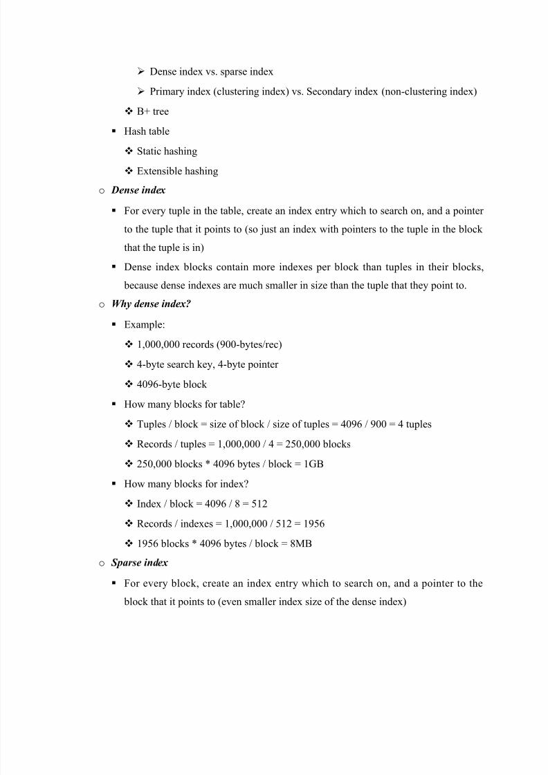
o Dense index

For every tuple in the table, create an index entry which to search on, and a pointer

to the tuple that it points to (so just an index with pointers to the tuple in the block

that the tuple is in)

Dense index blocks contain more indexes per block than tuples in their blocks, because dense indexes are much smaller in size than the tuple that they point to.

o Why dense index?

Example:

1,000,000 records (900-bytes/rec)

4-byte search key, 4-byte pointer

4096-byte block

How many blocks for table? Tuples / block = size of block / size of tuples = 4096 / 900 = 4 tuples

Records / tuples = 1,000,000 / 4 = 250,000 blocks

250,000 blocks * 4096 bytes / block = 1GB

How many blocks for index?

Index / block = 4096 / 8 = 512

Records / indexes = 1,000,000 / 512 = 1956

1956 blocks * 4096 bytes / block = 8MB

o Sparse index

For every block, create an index entry which to search on, and a pointer to the

block that it points to (even smaller index size of the dense index)



In real world, this reduces the index size dramatically, because there may be many

tuples in one block, for which sparse index only creates on index entry to those

tuples

o Sparse 2nd level

For every index block, create an index entry which to search on, and a pointer to

the index block that it points to (an index on the index, which further reduces in

size)

Can create multiple level of indexes (multi-level index)

o Terms

Index sequential file (Index Sequential Access Method)

Search key (≠ primary key)

Dense index vs. Sparse index

Multi-level index

o Duplicate keys

Dense index, one way to implement – Create an index entry for each tuple

Dense index, typical way – Create an index entry for each unique tuple

o Updates on the index?

Insertion (empty) – First follow the link structure to identify where the tuple should

be located (found with enough space)

Insertion (overflow) – Create an overflow block with a pointer from the original

block, which adds the entry 15 into the overflow block

Insertion (redistribute)

Try to move blocks to other adjacent blocks

Update any changes to the indexes as needed

o Deletion (one tuple)

See which index block the tuple is located

If the first entry of the block is not deleted, no update to index necessary

If the first entry of the block is deleted, update the index appropriately



o Deletion (entry block)

If the entire block is deleted, the index entry can be deleted

Move all index entries within the block up to compact space

o Primary index – Index that is created over the set of attributes that the table is

stored (also called clustering index)

o Secondary index

Index on a non-search-key

Unordered tuples – Non-sequential file

Sparse index make sense?

Does not make sense because the files are not not in sequence

Dense index on first level

Sparse index from the second level

o Duplicate values & secondary indexes

One option – Dense index for every tuple that exist

Buckets

Blocks that holds pointers to the same index keys

Intermediary level between the index and the tables

o Traditional index

Advantage

Simple

Sequential blocks

Disadvantage

Not suitable for updates

Becomes ugly (loses sequenality and balance) over time

B+ tree

o B+ tree

Most popular index structure in RDBMS

Advantage

Suitable for dynamic updates



Balanced

Minimum space usage guarantee

Disadvantage

Non-sequential index blocks

o B+ tree example

N pointers, (n-1) keys per node

Keys are sorted within a node

Balanced: all leaves at same level

o Same non-leaf node (n = 3)

At least n/2 pointers (except root)

At least 2 pointers in the root

o Nodes are never too empty

Use at least

Non-leaf: n/2 pointers

Leaf: (n-1)/2 +1 pointers

o Insert into B+ tree (simple case)

o Insert into B+ tree (leaf overflow)

Split the leaf, insert the first key of the new node

Move the second half to a new node

Insert the first key of the new node to the parent

o Insert into B+ tree (non-leaf overflow)

Find the middle key

Move everything on the right to a new node

Insert (the middle key, the pointer to the new node) into the parent

o Insert into B+ tree (new root node)

Insert (the middle key, the pointer to the new node) into the new root

o Delete from B+ tree (simple case)

Underflow (n = 4)

Non-leaf < n/2 = 2 pointers



Leaf < (n-1)/2 +1 = 3 pointers

o Delete from B+ tree (coalesce with sibling)

Move the node across to its sibling if there are rooms available

o Delete from B+ tree (re-distribute)

Grab a key from the sibling and move it to the underflowing node

o Delete from B+ tree (coalesce at non-leaf)

Push down the parent key into the child node

Get the mid-key from parent

Push down one of the grand-parent keys into the neighboring parent key

Point the child key to the push-down grand-parent key

o Delete from B+ tree (redistribute at non-leaf)

Combine the parent and the neighboring keys to make one full node

Push down one of the grand-parent keys

Push up one of the neighboring parent keys

o B+ tree deletions in practice

Coalescing is often not implemented

Too hard and not worth it!

o Question on B+ tree

SELECT *

FROM Student

WHERE sid > 60

Very efficient on B+ tree

Not efficient with hash tables

o Index creation in SQL

CREATE INDEX ON <table> (<attr>, <attr>, …)

i.e.,

CREATE INDEX ON

Student (sid)

Creates a B+ tree on the attributes



Speeds up lookup on sid

Clustering index (in DB2)

CREATE INDEX ON

Student (sid) CLUSTER

Tuples are sequenced by sid

Hash table

o What is a hash table?

Hash table

Hash function

Divide the integer by the key

h(k): key →integer [0…n]

i.e., h(‘Susan’) = 7

Array for keys: T[0…n]

Given a key k , store it in T[h(k)]

Properties

Uniformity – entries are distributed across the table uniformly

Randomness – even if two keys are very similar, the hash values will eventually

be different

o Why hash table?

Direct access

saved space – Do not reserve a space for every possible key

o Hashing for DBMS (static hashing)

Search key → h(key), which points to a (key, record) in disk blocks (buckets)

o Record storage

Can store as whole record or store as key and pointer, which points to the record

o Overflow

Size of the table is fixed, thus there is always a chance that a bucket would

overflow

Solutions:



Overflow buckets (overflow block chaining) – link to an additional overflow

bucket

More widely used

Open probing – go to the next bucket and look for space

Not used very often anymore

o How many empty slots to keep?

50% to 80% of the blocks occupied

If less than 50% used

Waste space

Extra disk look-up time with more blocks that needs to be looked up

If more than 80% used Overflow likely to occur

o Major problem of static hashing

How to cope with growth?

Data tends to grow in size

Overflow blocks unavoidable

o Extensible hashing

Two ideas

Use i of b bits output by hash function

Use the prefix of the first i bits of a string of b-bits in length (i.e., use the first

3 bits of a 5-bit hash value)

Use directory that maintains pointers to hash buckets (indirection)

Maintain a directory and do some indirection

Possible problems

When there are many duplicates, because there are more copies than digits (?)

Still need to use overflow buckets

No space occupancy guarantee when values are extremely skewed, thus needing

a very good hash function



Efficient for equality operator (=), but not efficient for range operators (>, <,

etc.)

Bucket merge

Bucket merge condition

Bucket i’s are the same

First (i-1) bits of the hash key are the same

Directory shrink condition

All bucket i’s are smaller than the directory i

Summary

Can handle growing files

No periodic reorganizations

• Indirection

Up to 2 disk accesses to access a key

• Directory doubles in size

Not too bad if the data is not too large

Extendible Hashing

o Data Structure

Use the first i of b bits output by the hash function to identify each record

Use a directory that maintains pointers to hash buckets (indirection)

o Queries and Updates

To locate the bucket, look up the first i bits and traverse the directory using those

bits

To insert into a bucket, use the first i bits and traverse the directory using those bits

to the appropriate bucket

If there is space in the bucket, insert the record into the bucket

If there is no space in the bucket, and the i digit of the bucket address table is

equal to the bucket i digit

Only one entry in the bucket address table points to the bucket



Increase both the i digit of the bucket address table and the i digit of the

bucket by 1, and split the bucket into two, and insert into the appropriate

bucket

If there is no space in the bucket, and the i digit of the bucket address table is

greater then the i digit of the bucket

More than one entry in the bucket address table points to the bucket

Redirect one of the entries in the bucket address table to point to a new

bucket, and increase the i digit current bucket by 1

Join Algorithms

o Givens

10 tuples/block

Number of tuples in R (|R|) = 10,000

Number of blocks for table R (BR ) = |R| / (tuples/block) = 10,000 / 10 = 1,000

blocks in R

Number of tuples in R (|S|) - 5,000

Number of blocks for table S (BS) = |S| / (tuples/block) = 5,000 / 10 = 500 blocks in

S

Number of buffer blocks in main memory (M) = 102

o Block Nested-Loop Join

Steps:

Read a number of blocks into main memory (using M – 1 blocks)

Read the blocks of another table one by one into main memory (using one

block)

Compare and output the joined tuples (using 1 block)

Repeat until done

Example:

Since main memory is too small to hold either table, we should use the memory

to hold as many blocks of the larger table, and leave the smaller table on the

outside.

Main memory usage



102 main memory blocks – 100 blocks (S), 1 block (R), 1 block (writing output)

I/O count:

For S, read 100 blocks into memory at a time =

100

500= 5

For R, read 1 block into memory at a time = 1,000

Total I/O = 500000,1100

500

2+⋅

=+⋅

−S R

S B B

M

B= 5,500

o Merge Join

Steps:

If the tables are already sorted, can proceed straight into the merging and

compare part of the algorithm

If the tables are not sorted, sort each table first using merge sort, then merge and

compare the two tables

To sort:

o Read M blocks into main memory, sort them, then output it to a resultant

partition

o Repeat until done

To merge:

o Read the first blocks of the first M partitions (if less than or equal to M

partitions), or the first blocks of the first M – 1 partitions (if more than M

partitions, with one block for writing the output) into main memory, sort

them, then output it to a resultant partition

o Repeat until done

Example:

Main memory usage

M blocks are used in the splitting stage

In the first pass of the merging stage (while sorting the tables), M blocks are

used to store the blocks from the table

In the second pass and on of the merging stage (while sorting the tables), M

– 1 blocks are used to store the blocks from the table



Sorting the R table

Number of partitions =

102

000,1= 10

Splitting pass

Resulting in 10 partitions

Merging pass

Resulting in one sorted table

I/O for sorting = number of passes * (2 * number of blocks in the table = 2 *

(2 * 1,000) = 4,000

Sorting the S table

Number of partitions =

102

500= 5

Splitting pass

Resulting in 10 partitions

Merging pass

Resulting in one sorted table

I/O for sorting = number of passes * (2 * number of blocks in the table = 2 *

(2 * 500) = 2,000

Merging

I/O for merging = BR + BS = 1,000 + 500 = 1,500

Total I/O = Sorting + Merging = (4,000 + 2,000) + 1,500 = 7,500

o Hash Join

Steps:

Hashing (bucketizing)

Split the tables into M – 1 buckets

Joining

Read buckets from each table into main memory and see which tuples in the

buckets match

Example:



o For every R tuples, disk I/O = C + J (assume that disk blocks are not

clustered)

Example:

Given: J = 0.1, BI (number of index blocks) = 90

Load index into main memory (because index will be accessed multiple times,

and it is smaller than the main memory size) = BI = 90

Therefore, the index lookup variable C is 0, because the whole index is in

main memory.

For every tuple in R, look up the tuple in S = |R| * (C + J)

For every block in R = BR

Total I/O = BI + (BR + |R| * (C + J)) = 90 + (1,000 + 10,000 (0 + 0.1)) = 2,090

Example:

Given: J = 1, BI = 200

Main memory usage:

Cannot load index into main memory, because it is bigger than the number of

buffer blocks in main memory

Load as many index blocks into main memory

102 blocks – 1 block for reading R table, 1 block for reading S table, 1 block

for writing output, 1 block for index node, 98 blocks for index leaf nodes

Therefore, the index lookup variable C ≈ 0.5 (98/199 and 101/199 for the

two cases), since only the root of the index and 98 leaf nodes can be in the

main memory

Total I/O = BI + (BR + |R| * (C + J)) = 99 + (1,000 + 10,000 * (0.5 + 1)) =

16,099

Relational Design Theory

o Problems with redundancy: Update anomalies

Modification anomaly – A situation in which the modification of a row of a table

creates an inconsistency with another row

i.e., modifying the class that a student is taking



Deletion anomaly – A situation in which the deletion of one row of a table results

in the deletion of an unintended information

i.e., deleting a class may also delete information about a student (if that is the

last entry of the student in the database)

Insertion anomaly – A situation in which the insertion of a row in a table creates an

inconsistency with other rows

i.e., inserting a new class must also include student information for students in

that class

o Functional Dependency

Definition: Given A1, A2, ..., An, we can uniquely determine B1, B2, ..., Bm

Trivial functional dependency: A →B, and B ⊆ A

Completely non-trivial functional dependency: A →B, X ∩ Y = ∅

Logical implication

Example: R ( A, B, C, G, H I )

Functional dependencies:

o A →B

o A →C

o CG →H

o CG →I

o B →H

Conclusions:

o A →BCH, because A →ABCH

o CG →HI, because CG →CGHI

o AG →I, because AG →ABCGHI

o A does not →I, because A →BCH

Canonical cover

Functional dependencies

A →BC

B →C



A →B

AB →C

Is A →BC necessary?

No, because A →B, and B →C, so A →BC, thus A →BC is not necessary Is AB →C necessary?

No, because B →C, so AB →is not necessary

Canonical cover may not be unique

Most of the time, people directly find a canonical cover by intuition

Closure (of attribute set)

CLOSURE OF X: X+. the set of all attributes functionally determined by X

Algorithm for closure computation:

start with T = X

repeat until no change in T

if T contains LHS of a FD, add RHS of the FD to T

Example:

F =

o A →B

o A →C

o CG →H

o CG →I

o B →H

{A}+ = {A, B, C, H}

{AG}+ = {A, B, C, G, H, I}

Example: StudentClass

{sid}+ = sid, name,

Key & functional dependency

Notes:

A key determines a tuple

Functional dependency determines other attributes



X is a key of R if

X →all attributes of R (ie, X+ = R)

No subset of X satisfies the prior property mentioned above (i.e., X is

minimal)

o Decomposition

Notes:

To obtain a "good" schema, we often split a table into smaller ones

Split table R(A1, ..., An) into R1(A1, ..., Ai) and R2(Aj, ..., An)

{A1, ... An} = {A1, .., Ai} UNION {Aj, ..., An}

Why do we need common attributes?

So we can put the tables back together to form the original table Lossless decomposition

Definition

We should not lose any information by decomposing R

R = R1 NJ R2

Example:

cnum sid name

143 1 James143 2 Jane

325 2 Jane

What if we use the following schema? R1 ( cnum, sid ), R2 ( cnum, name )

o Not lossless decomposition, we get additional answers not in the original

table

What if we use the following schema? R1 ( cnum, sid ), R2 ( sid, name )

o It is a lossless decomposition, because sid → name, so the common

attribute uniquely determines a tuple in the R2 table

When is decomposition lossless?

Common attribute should uniquely determine a tuple in at least one table

R ( X, Y, Z ) →R1 ( X, Y ), R2 ( Y, Z ) is loss iff either Y →Z or Y →X



Example: ClassInstructor ( dept, cnum, instructor, office, fax )

FDs:

o dept, cnum →instructor

o

instructor →officeo office →fax

Decomposed tables:

o R1 ( dept, cnum, instructor, office )

R3 ( instructor, office )

R4 ( dept, cnum, instructor )

o R2 ( office, fax )

o Boyce-Codd Normal Form (BCNF)

Definition: R is in BCNF with regard to F, iff for every non-trivial X → Y, X

contains a key

No redundancy due to FD

Algorithm:

For any R in the schema

If (X → holds on R AND

X → Y is non-trivial AND

X does not contain a key), then

1) Compute X (X : closure of X)

2) Decompose R into R1 (X+) and R2 (X, Z)

// X becomes common attributes

// Z: all attributes in R except X+

Repeat until no more decomposition

Example: StudentAdvisor ( sid, sname, advisor )

FDs:

o sid →sname

o sid →advisor



Is it BCNF?

o Dependency-preserving decomposition

FD is a kind of constraint

Checking dependency preserving decomposition Example: R ( office, fax ), office →fax

A local checking operation: look up office in the table, and make sure the

newly inserted fax number is the same

Example: R1 ( A, B ), R2 ( B, C ), A →B, B →C, A →C

Check for each part of the tuple corresponding to each table to make sure that

it does not violate any constraints

Do not need to check A→

C because it is implied where A→

B and B→

C Example: R1 ( A, B ), R2 ( B, C ), A →C

Have to join tables together to make sure that the attributes are not duplicated

BCNF does not guarantee dependency preserving decomposition

Example: R ( street, city, zip ), street, city →zip, zip →city

Use violating FD to split up table

o R1 ( zip, city )

o R2 ( zip, street )

Have to join the two tables together in order to check whether street, city →

zip

o Third-Normal Form (3NF)

Definition: R is in 3NF regards to F iff for every non-trivial X → Y, either

1. X contains a key, or

2. Y is a member of key

Theorem: There exist a decomposition in 3NF that is a dependency-preservingdecomposition

May have redundancy, because of the relaxed condition

o Multivalue dependency (MVD)

Example: Class(cnum, ta, sid). Every TA is for every student



Table:

cnum: 143, TA: tony, james, sid: 100, 101, 103

cnum: 248, TA: tony, susan, sid: 100, 102

cnum ta sid-------------------------------

143 tony 100

143 tony 101

143 tony 103

143 james 100

143 james 101

143 james 103

248 tony 100

248 tony 102

248 susan 100

248 susan 102

Where does the redundancy come from?

In each class, every TA appears with every student

o For C1, if TA1 appears with S1, TA2 appears with S2, then TA1 also

appears with S2

Definition: X →> R

For every tuple u, v in R

if u[x] = v[x], then there exist a tuple w such that

1. w[X] = u[X] = v[X]

2. w[Y] = u[Y]

3. w[Z] = v[Z]

where Z is all attributes in R except (X, Y)

MVD requires that tuples of a certain form exist

X →> Y means that if two tuples in R agree on X, we can swap Y values of the

tuples and the two new tuples should still exist in R.



Complementation rule: Given X →> Y, if Z is all attributes in R except (X, Y), then

X →> Z

MVD as a generalization of FD

If X →Y, then X →> Yo Fourth Normal Form (4NF)

Definition: R is in 4NF iff for every non-trivial MVD X →> Y, X contains a key

Since every FD is a MVD, 4NF implies BCNF

Decomposition algorithm for 4NF

For any R in the schema

If non-trivial X →> Y holds on R, and if X does not have a key

Decompose R into R1(X, Y) and R2(X, Z)// X is common attributes

where Z is all attributes in R except X

Repeat until no more decomposition

o Summary

4NF →BCNF →3NF

4NF

Remove redundancies from MVD, FD

Not dependency preserving

BCNF

No redundancies from FD

Not dependency preserving

3NF

May have some edundancies

Dependency preserving. BCNF may not lead to a unique decomposition when there the dependency graph

cannot be represented using a tree structure

Transactions and concurrency control

Transaction – Sequence of SQL statements that is considered as a unit



Example:

Transfer $1M from Susan to Jane

S1:

UPDATE Account

SET balance = balance – 1,000,000

WHERE owner = ‘Susan’

S2:

UPDATE Account

SET balance = balance + 1,000,000

WHERE owner = ‘Jane’

Increase Tony’s salary by $100 and by 40%

S1:

UPDATE Employee

SET salary = salary + 100

WHERE name = ‘Tony’

S2:

UPDATE Employee

SET salary = salary * 1.4

WHERE name = ‘Tony

Transactions and ACID property

ACID property

Atomicity: “ALL-OR-NOTHING”

o Either ALL OR NONE of the operations in a transaction is executed.

o If the system crashes in the middle of a transaction, all changes by the

transaction are "undone" during recovery.

Consistency: If the database is in a consistent state before a transaction, the

database is in a consistent state after the transaction

Isolation: Even if multiple transactions are executed concurrently, the result

is the same as executing them in some sequential order



o Each transaction is unaware of (is isolated from) other transaction running

concurrently in the system

Durability

o If a transaction committed, all its changes remain permanently even after

system crash

With AUTOCOMMIT mode OFF

Transaction implicitly begins when any data in DB is read or written

All subsequent read/write is considered to be part of the same transaction

A transaction finishes when COMMIT or ROLLBACK statement is executed

o COMMIT: All changes made by the transaction is stored permanently

o ROLLBACK: Undo all changes made by the transaction

With AUTOCOMMIT mode ON

Every SQL statement becomes one transaction is committed

Serializable schedule

Example in handout

Schedule A

o T1

Read(A); A ← A + 100;Write(A);

Read(B); B ← B + 100;

Write(B);

o T2

Read(A); A ← A x 2;

Write(A);

Read(B); B←

B x 2;Write(B);

o Result = 250 vs. 250, database is still in a consistent state

Schedule B (switch the order that the transactions are executed)



o T2

Read(A); A ← A x 2;

Write(A);

Read(B); B ← B x 2;

Write(B);

o T1

Read(A); A ← A + 100;

Write(A);

Read(B); B ← B + 100;

Write(B);


It is the job of the application to make sure that the transactions gets to the

database in the correct order

Schedule C (inter-mingled statements)

o T1

Read(A); A ← A + 100;

Write(A);

o T2

o Read(A); A ← A x 2;

Write(A);

o T1

Read(B); B ← B + 100;

Write(B);

o T2


Write(B);


Schedule D (inter-mingled statements)



o T1

Read(A); A ← A + 100;

Write(A);

o T2


Write(A);


Write(B);

o T1

Read(B); B ← B + 100;

Write(B);

o Result = 250 vs. 150, database is NOT in a consistent state

Schedule E (inter-mingled statements)

o T1

Read(A); A ← A + 100;

Write(A);

o T2


Write(A);


Write(B);

o T1

Read(B); B ← B + 100;

Write(B);


Simplifying assumption

The "validity" of a schedule may depend on the initial state and the particular

actions that transactions take

o It is difficult to consider all transaction semantics



We want to identify "valid" schedules that give us the "consistent" state

regardless of

o the initial state

o 2) transaction semantics

We only look at database read and write operation and check whether a

particular schedule is valid or not.

o Read/write: input/output from/to database

o The only operations that can screw up the database

o Much simpler than analyzing the application semantics

Notation

Sa = r1(A) w1(A) r1(B) w1(B) r2(A) w2(A) r2(B) w2(B)

o Subscript 1 means transaction 1

o r(A) means read A

o w(A) means write to A

Schedule A: Sa = r1(A) w1(A) r1(B) w1(B) r2(A) w2(A) r2(B) w2(B)

o SERIAL SCHEDULE: all operations are performed without any

interleaving

Schedule C: Sc = r1(A) w1(A) r2(A) w2(A) r1(B) w1(B) r2(B) w2(B)o COMMENTS: Sc is good because Sc is "equivalent" to a serial schedule

Schedule D: Sc = r1(A) w1(A) r2(A) w2(A) r2(B) w2(B) r1(B) w1(B)

o Dependency in the schedule

w1(A) and r2(A): T1 -> T2

w2(B) and r1(B): T2 -> T1

o Cycle. T1 should precede T2 and T2 should precede T1

o Cannot be rearranged into a serial schedule

o Is not "equivalent" to any serial schedule

Conflicting actions: A pair of actions that may give different results if swapped

Conflict equivalence: S1 is conflict equivalent to S2 if S1 can be rearranged into

S2 by a series of swaps of non-conflicting actions



Conflict serializability: S1 is conflict serializable if it is conflict equivalent to

some serial schedule

A “good” schedule

Precedence graph P(S)

Nodes: transactions in S

Edges: Ti →Tj if

o pi(A), qj(A) are actions in S

o 2) pi(A) precedes qj(A)

o 3) At least one of pi, qj is a write

P(S) is acyclic ⇔S is conflict serializable

Summary: Good schedule: conflict serializable schedule

Conflict serializable <=> acyclic precedence graph

Recoverable/cascadeless schedule

Recoverable schedule: Schedule S is RECOVERABLE if Tj reads a data item

written by Ti, the COMMIT operation of Ti appears before the COMMIT

operation of Tj

Cascadeless schedule: A single transaction abort leads to a series of transactionrollback

o Transaction

Sequence of SQL statements that is considered as a unit

Motivation

Crash recover

Concurrency

Transactions and ACID property

ACID property

Atomicity: “ALL-OR-NOTHING”

o Either ALL OR NONE of the operations in a transaction is executed.



o If the system crashes in the middle of a transaction, all changes by the

transaction are "undone" during recovery.

Consistency: If the database is in a consistent state before a transaction, the

database is in a consistent state after the transaction

Isolation: Even if multiple transactions are executed concurrently, the result

is the same as executing them in some sequential order

o Each transaction is unaware of (is isolated from) other transaction running

concurrently in the system

Durability

o If a transaction committed, all its changes remain permanently even after

system crash

Main questions:

What execution orders are "valid"?

o We first need to understand what execution orders are okay

Serializability, Recoverability, Cascading rollback

How can we allow only "valid" execution order?

o Concurrency control mechanism

Serializable and conflict serializable schedules

Simplifying assumption

We only look at database read and write operation and check whether a

particular schedule is valid or not.

o Read/write: input/output from/to database

o The only operations that can screw up the database

o Much simpler than analyzing the application semantics

Definition: All operations are performed without any interleaving

Is r1(A) w1(A) r2(A) w2(A) r1(B) w1(B) r2(B) w2(B) a serializable

schedule?

o No, r1(B) w1(B) of transaction 1 went after r2(A) w2(A) of transaction 2,

which makes transaction 1 and transaction 2 interleaving

Dependencies in the schedule



Example: r1(A) w1(A) r2(A) w2(A) r2(B) w2(B) r1(B) w1(B)

o w1(A) and r2(A): T1 → T2

w2(B) and r1(B): T2 →T1

Cycle. T1 should precede T2 and T2 should precede T1

Cannot be rearranged into a serial schedule

Is not "equivalent" to any serial schedule

Some sequence of operations cause dependency

A schedule is bad if we have a cycle in the dependency graph

Without a cycle, the schedule is "equivalent" to a serial schedule

Conflicting actions: A pair of actions that may give different results if swapped

Conflict equivalence: S1 is conflict equivalent to S2 if S1 can be rearranged into

S2 by a series of swaps of non-conflicting actions

Conflict serializability: S1 is conflict serializable if it is conflict equivalent to

some serial schedule

A “good” schedule

Precedence graph P(S)

Nodes: transactions in S

Edges: Ti →Tj if

o pi(A), qj(A) are actions in S

o 2) pi(A) precedes qj(A)

o 3) At least one of pi, qj is a write

P(S) is acyclic ⇔S is conflict serializable

Recoverable and cascadeless schedules

Recoverable schedule: Schedule S is recoverable if Tj reads a data item written

by Ti, the commit operation of Ti appears before the COMMIT operation of Tj

Cascadeless schedule: A schedule S is cascadeless if Tj is a data item written by

Ti the commit operation of Ti appears before Tj read

Cascading rollback: T2 depends on data from T1, and if T1 is aborted, T2 is

aborted



Dirty reads – data is read from an uncommitted transaction

Relationship between different schedules?

Serial →conflict serializable

Serial →recoverable Serial →cascadeless

Serial guarantees read/write/commit actions of one transaction are all

grouped together, thus transactions are cascadeless

Cascadeless →recoverable

The commit action is guaranteed to be before the read/write actions

Example: w1(A) w1(B) w2(A) r2(B) c1 c2

Not serial

Conflict serializable

Recoverable

Not cascadeless

Example: w1(A) w1(B) w2(A) c1 r2(B) c2

Not serial

Conflict serializable

Recoverable

Cascadeless

o Two-phase locking

Main objective: Achieve serializable and cascadeless schedule

Why do we have cascading rollback? How can we avoid it?

Dirty read

Basic idea:

Before T1 writes, T1 obtains a lock

2) T1 releases the lock only when T1 commits

3) No one else can access the tuple/object when T1 has the lock

What should T2 do before read?

Obtain a lock before a read. Release it after the read



Potential locking protocol

Rules

Rule (1): Ti lock a tuple before any read/write

Rule (2): If Ti holds the lock on A, Tj cannot access A (j != i)

Rule (3): After write, release the lock at commit, after read, release the lock

immediately

Does it guarantee conflict-serializability?

Example:

o T1 T2

r(A)

w(A)

w(A)

o Is it conflict serializable?

No, because are dependencies between r1(A) and w2(A), and w2(A) and w1(A)

o How can we avoid this problem?

Keep the lock until the end of the transaction

Rigorous Two Phase Locking Protocol

Rules: Rule (1): Ti locks a tuple before any read/write


Rule (3): Release all locks at the commit

Theorem: Rigorous 2PL ensures conflict-serializable and cascadeless schedule.

Rigorous 2PL schedule: schedules that can be produced by rigorous 2PL

schedule

Two Phase Locking Protocol: Less strict locking protocol than rigorous 2PL Rules

Rule (1): Ti lock a tuple before any read/write


Rule (3): Two stages:



o growing stage: Ti may obtain locks, but may not release any lock

o shrinking stage: Ti may release locks, but my not obtain any lock

Theorem: 2PL ensures a serializable schedule

Shared & exclusive lock Separate locks for read and write

Shared lock:

Lock for read

Multiple transactions can obtain the same shared lock

Exclusive lock

Lock for write

If Ti holds an exclusive lock for A, no other transaction can obtain a

shared/exclusive lock on A

r(A), r(A): allowed, w(A), r(A): disallowed

Before read, Ti requests a shared lock

Before write, Ti requests an exclusive lock

The remainder is the same as 2PL or rigorous 2PL

Compatibility matrix

Shared Exclusive (trying to get lock)

Shared Yes No

Exclusive No No

Rigorous 2PL with shared lock → conflict serializable and cascadeless 2PL

with shared lock →conflict serializable

One more problem: Phantom

Tuples are inserted into a table during a transaction

Does it follow rigorous 2PL?

o Yes

Why do we get this result?

o T1 reads the "entire table" not just e3



o Before T1 reads e3, T1 should lock everything before e3 (ie, e1), so that

"scanned part" of the table does not change

T1 has to worry about "non-existing" tuple: PHANTOM PHENOMENON

Solution:

o When T1 reads tuples in table R, do not allow insertion into R by T2

o T2 may update existing tuples in R, as long as it obtains proper exclusive

locks

The problem is from insertion of NEW tuples that T1 cannot lock

INSERT LOCK on table

o Before insertion, Ti gets an exclusive insert lock for the table

o (2) Before read, Ti gets a shared insert lock for the table

Same compatibility matrix as before

NOTE: Ti should still obtain shared/exclusive lock for every tuple it

reads/writes

o Transactions in SQL

To be filled in…

exam notes COA

Documents

Transcript of exam notes COA