1

EXAKT

SKF

Phase 1, Session 2

Principles

2

The CBM Decision supported by EXAKT

Given the condition today, the asset mgr. takes one of three decisions:

1. Intervene immediately and conduct maintenance on an equipment at this time, or to

2. Plan to conduct maintenance within a specified time, or to

3. Defer the maintenance decision until the next CBM observation

3

The conventional CBM decision method from Nowlan & Heap, (Moubray)

Co

nd

itio

n

Working age

P-F Interval

Detectable indication of a failing process

Detection of the potential failure

CBM inspection interval:

Potential failure, P

< P-F Interval

Net P-F Interval

Functional failure, F

4

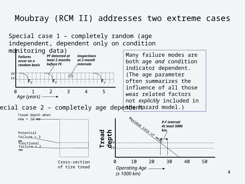
Moubray (RCM II) addresses two extreme cases

F2 F3 F1

0 2 3 4 51

Failures occur on a random basis

Inspections at 2 month intervals

PF detected at least 2 months before FF.

PFFF

Age (years)

Special case 1 – completely random (age independent, dependent only on condition monitoring data)

0 20 30 40 5010Operating Age(x 1000 km)

PF

FFTre

ad

d

ep

thSpecial case 2 – completely age dependent

P-F intervalAt least 5000 km

Maximum rate of wear

Tread depth when new = 12 mm

Potential failure = 3 mm

Functional failure = 2 mm

Cross-section of tire tread

Many failure modes are both age and condition indicator dependent. (The age parameter often summarizes the influence of all those wear related factors not explicitly included in the hazard model.)

5

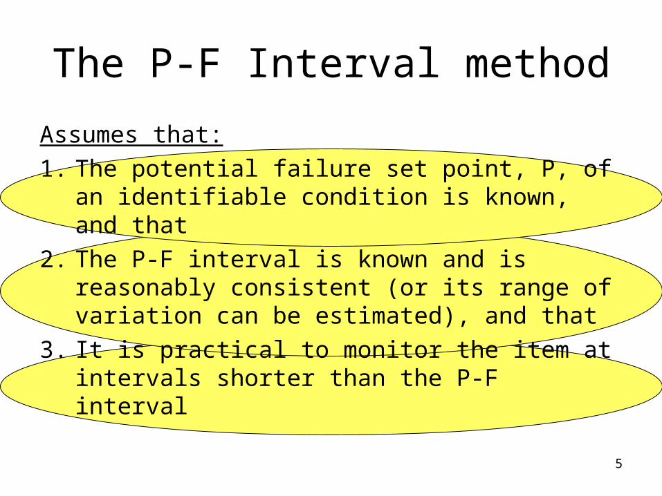
The P-F Interval method

Assumes that:

1. The potential failure set point, P, of an identifiable condition is known, and that

2. The P-F interval is known and is reasonably consistent (or its range of variation can be estimated), and that

3. It is practical to monitor the item at intervals shorter than the P-F interval

6

EXAKT has two ways of deciding whether an item is in a “P” state

1. A decision based solely on failure probability.

2. A decision based on the combination of failure probability and the quantifiable consequences of the failure, and

7

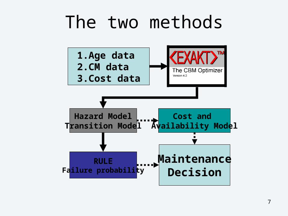
The two methods

1. Age data2. CM data3. Cost data

Hazard ModelTransition Model

RULEFailure probability

MaintenanceDecision

Cost and Availability Model

8

Assumptions and models used in EXAKT

9

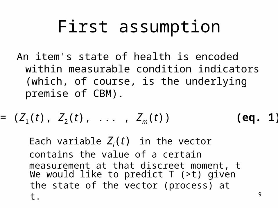
First assumption

An item's state of health is encoded within measurable condition indicators (which, of course, is the underlying premise of CBM).

Z(t) = (Z1(t), Z2(t), ... , Zm(t)) (eq. 1)

Each variable Zi(t) in the vector contains the value of

a certain measurement at that discreet moment, t

We would like to predict T (>t) given the state of the vector (process) at t.

10

2nd assumption

),,,(,0,0

),,);(,(

21

)(1

1

m

tZm

iiet

tZth

where β is the shape parameter, η is the scale parameter, and γ is the coefficient vector for the condition monitoring variable (covariate) vector. The parameters β, η, and γ, will need to be estimated in the numerical solution.

11

3rd assumption

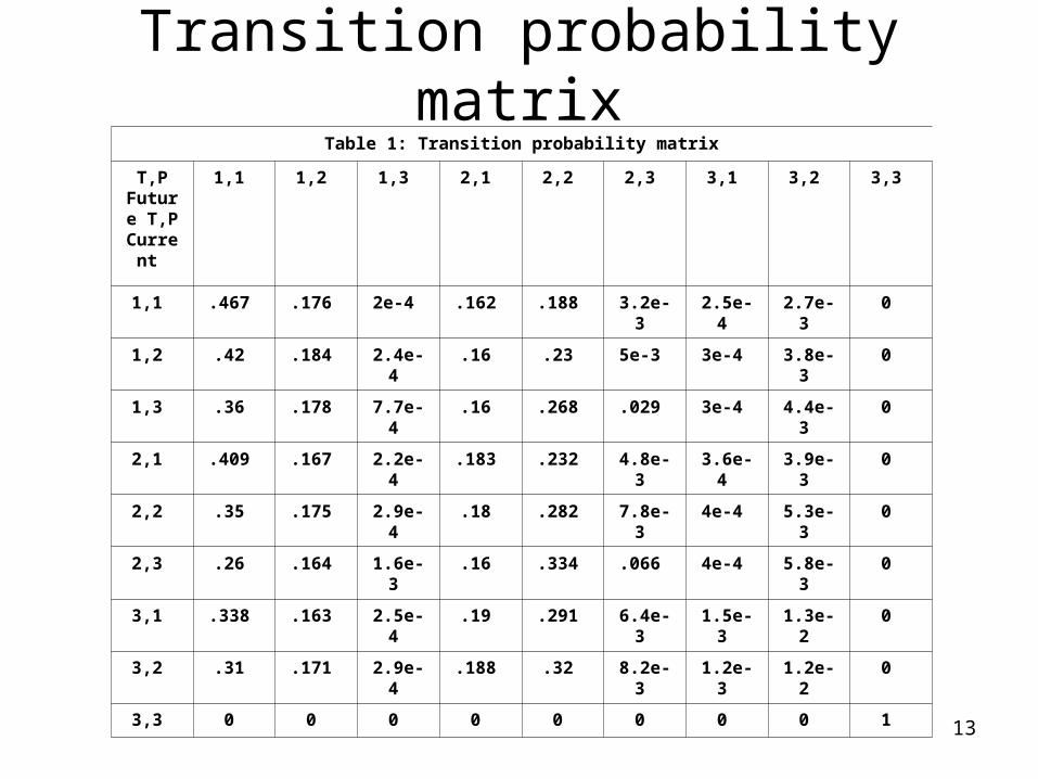
In EXAKT, it is assumed that Z(d)(t) follows a non-homogeneous Markov failure time model described by the transition probabilities

Lij(x,t)=P(T>t, Z(d)(t)= Rj(z)|T>x, Z(d)(x)= Ri

(z)) (eq. 3)

where:x is the current working age,t (t > x) is a future working age, andi and j are the states of the covariates at x and t respectivelyZ(d)(t) is the vector of “representative” values of each condition indicator.

It is the probability that the item survives until t and the state of Z(d)(t) is j given that the item survives until x and the previous state, Z(d)(x) , was i. The transition behavior can then be displayed in a Markov chain transition probability matrix, for example, that of the next slide.

12

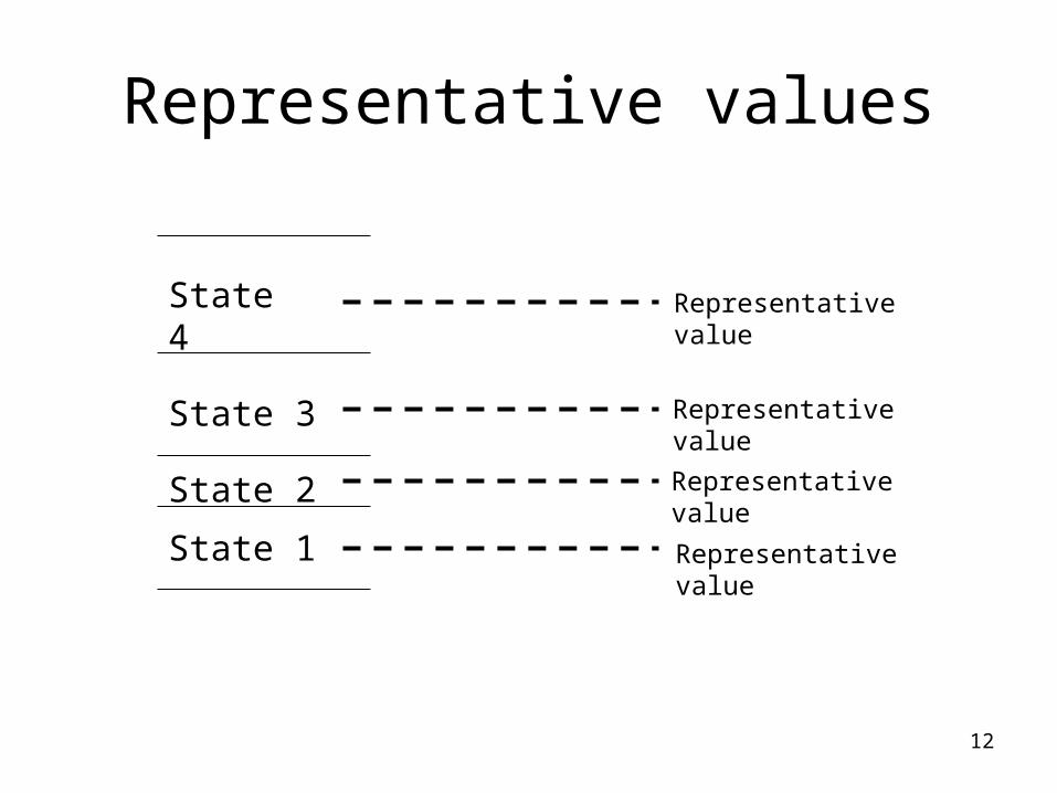
Representative values

State 4

State 3

State 2

State 1

Representative value

Representative value

Representative value

Representative value

13

Transition probability matrixTable 1: Transition probability matrix

T,P Future

T,P Curren

t

1,1 1,2 1,3 2,1 2,2 2,3 3,1 3,2 3,3

1,1 .467 .176 2e-4 .162 .188 3.2e-3 2.5e-4 2.7e-3 0

1,2 .42 .184 2.4e-4 .16 .23 5e-3 3e-4 3.8e-3 0

1,3 .36 .178 7.7e-4 .16 .268 .029 3e-4 4.4e-3 0

2,1 .409 .167 2.2e-4 .183 .232 4.8e-3 3.6e-4 3.9e-3 0

2,2 .35 .175 2.9e-4 .18 .282 7.8e-3 4e-4 5.3e-3 0

2,3 .26 .164 1.6e-3 .16 .334 .066 4e-4 5.8e-3 0

3,1 .338 .163 2.5e-4 .19 .291 6.4e-3 1.5e-3 1.3e-2 0

3,2 .31 .171 2.9e-4 .188 .32 8.2e-3 1.2e-3 1.2e-2 0

3,3 0 0 0 0 0 0 0 0 1

14

4th assumptionThe combined PHM and transition

models

For a short interval of time, values of transition probabilities can be approximated as:

Lij(x,x+Δx)=(1-h(x,Ri(z))Δx) • pij(x,x+ Δx) (eq. 6)

Equation 6 means that we can, in small steps, calculate the future probabilities for the state of the covariate process Z(d)(t). Using the hazard calculated (from Equation 2) at each successive state we determine the transition probabilities for the next small increment in time, from which we again calculate the hazard, and so on.

15

Making CBM decisions

Two ways

16

CBM decisions based on probability

The conditional reliability function can be expressed as:

( ) ( ( ) ) ( )ijj

R t x i P T t T x Z x i L x t (eq. 7)

The “conditional reliability” is the probability of survival to t given that

1.failure has not occurred prior to the current time x, and

2.CM variables at current time x are Ri(z)

Equation 7 points out that the conditional reliability is equal to the sum of the conditional transition probabilities from state i to all possible states.

17

Remaining useful life (RUL)

Once the conditional reliability function is calculated we can obtain the conditional density from its derivative. We can also find the conditional expectation of T - t, termed the remaining useful life (RUL), as                                                                       

(eq. 8)( ( )) ( ( ))t

E T t T t Z t R x t Z t dx

In addition, the conditional probability of failure in a short period of time Δt can be found as

tZtttRtZttTTtP dd ,|1,|

For a maintenance engineer, predictive information based on current CM data, such as RUL and probability of failure in a future time period, can be valuable for risk assessment and planning maintenance.

(eq. 9)

18

CBM decisions based on economics and probability

Control-limit policy: perform preventive maintenance at Td if Td < T; or

perform reactive maintenance at T if Td ≥ T,

Where:Td=inf{t≥0:Kh(t,Z(d)(t))≥d}

Where:K is the cost penalty associated with functional failure, h(t,Z(d)(t) is the hazard, and d (> 0) is the risk control limit for performing preventive maintenance. Here risk is defined as the functional failure cost penalty K times the hazard rate.

(Eq. 10)

19

The long-run expected cost of maintenance (preventive and reactive) per unit of working age will be:

)(

)(

)(

)())(1()(

dW

dKQC

dW

dQCdQCd pfp

(eq. 11)

where Cp is the cost of preventive maintenance, Cf = Cp+K is the cost of

reactive maintenance, Q(d)=P(Td≥T) is the probability of failure prior to a

preventive action, W(d)=E(min{Td,T}) is the expected time of

maintenance (preventive or reactive).

20

Best CBM policy

Let d* be the value of d that minimizes the right-hand side of Equation 11. It corresponds to T* = Td*. Makis and Jardine in ref. 3 have shown that for a non-decreasing hazard function h(t,Z(d)(t), rule T* is the best possible replacement policy (ref. 4).

Equation 10 can be re-written for the optimal control limit policy as:

T*=Td*=inf{t≥0:Kh(t,Z(d)(t))≥d*} (eq. 12)

For the PHM model with Weibull baseline distribution, it can be interpreted as (ref. 2))

1

min{ 0 ( ) ( 1) ln }m

i ii

T t Z t t

ln dK

(eq. 13)

Where

The numerical solution to Equation 13, which is described in detail in (Ref. 7) and (Ref. 8).

)(

)(

)(

)())(1()(

dW

dKQC

dW

dQCdQCd pfp

21

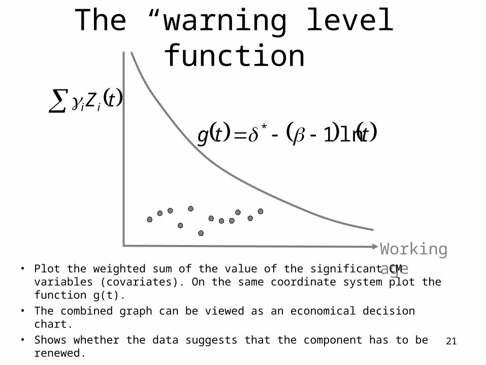
The “warning level” function

Working age

tZ ii

ttg ln1*

• Plot the weighted sum of the value of the significant CM variables (covariates). On the same coordinate system plot the function g(t).

• The combined graph can be viewed as an economical decision chart.

• Shows whether the data suggests that the component has to be renewed.

22

5th assumptionIn the decision chart, we approximate the value of

tZm

i

dii

1

tZm

iii

1

by

Decision chart

23

Numercal example

A CBM program on a fleet of Nitrogen compressors monitors the failure mode “second stage piston ring failure”. Real time data from sensors and process computers are collected in a PI historian. Work orders record the as-found state of the rings at maintenance.

The next four slides illustrate 4 EXAKT optimal CBM decisions

24

Decision 1- Only Probability

25

Decision 2-Probability and cost minimization

26

Decision 3-Probability and availability maximization

27

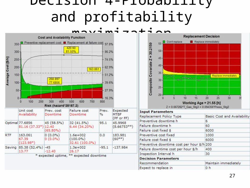
Decision 4-Probability and profitability maximization