Exact Maximum Likelihood Estimation of

Structured or Unit Root Multivariate

Time Series Models∗

Guy Melard† Roch Roy‡ Abdessamad Saidi§

CRM-3129June 2004

∗The authors thank Saıd Nsiri for helpful comments. This work has been partly funded by the co-operation betweenthe Commissariat general aux Relations internationales, Communaute Francaise Wallonie-Bruxelles and the Government ofthe Province of Quebec, with a grant from the Action de Recherche Concertee 96/01/201, Communaute Francaise Wallonie-Bruxelles, and IAP-network of the Belgian federal Government contract P51/24. It was also supported by grants from theNatural Science and Engineering Research Council of Canada, the Network of Centres of Excellence on The Mathematicsof Information Technology and Complex Systems (MITACS) and the Fonds quebecois de la recherche sur la nature et lestechnologies (FQRNT).

†ISRO and Faculty of Social Sciences, Politics and Economics, Universite Libre de Bruxelles, Campus Plaine, C.P. 210, Bddu Triomphe, B-1050 Bruxelles, Belgium (e-mail: gmelard@ulb.ac.be).

‡Departement de mathematiques et de statistique and Centre de recherches mathematiques, C.P. 6128, succ. Centre-ville,Montreal, Quebec, H3C 3J7, Canada (e-mail: royr@dms.umontreal.ca).

§Departement de mathematiques et de statistique, Universite de Montreal, C.P. 6128, succ. Centre-ville, Montreal, Quebec,H3C 3J7, Canada (e-mail: saidiabd@dms.umontreal.ca).

Abstract

The exact likelihood function of a Gaussian vector autoregressive-moving average (VARMA)model is evaluated in two non standard cases: (a) a parsimonious structured form, such asobtained in the echelon form structure or the scalar component model (SCM) structure; (b) apartially non stationary (unit root) model in error-correction form. The starting point is Shea’salgorithm (1987, 1989) for standard stationary and invertible VARMA models. Our algorithmalso provides the parameter estimates and their standard errors. The small sample propertiesof our algorithm were studied by Monte Carlo methods. Examples with real data are provided.

Keywords: Gaussian likelihood estimation, ARMA echelon form, Scalar component model,Cointegrated model, Kalman filter, Chandrasekhar-type recursions.

Resume

La fonction de vraisemblance gaussienne exacte d’un modele autoregressif-moyenne mobile vec-toriel (VARMA) est evalue dans deux cas non standard : (a) une representation parcimonieusestructuree comme la representation ARMA echelon ou celle des modeles a composantes scalaires(SCM) ; (b) la representation a correction d’erreur d’un modele partiellement non stationnaire(a racine unitaire). Le point de depart est l’algorithme de Shea (1987, 1989) pour l’estimationd’un modele VARMA standard, stationnaire et inversible. Notre algorithme fournit aussi lesestimations des parametres et leurs ecarts-type. Les proprietes de notre algorithme pour decourtes series ont ete etudiees par des methodes de Monte Carlo. Des exemples avec des don-nees reelles sont presentees.

1 Introduction

The purpose of this paper is to extend the exact maximum likelihood estimation procedure for the Gaus-sian vector autoregressive-moving average (VARMA) model when the model is stated in a parsimoniousstructured form or when the process has unit roots.

Stationary VARMA models of order (p, q) and dimension k are characterized by a large number ofparameters which are the k × k elements of the p + q coefficients plus the k(k + 1)/2 elements of theinnovation covariance matrix. Some elements of the coefficient matrices may be specified (e.g. to equalzero) without effect on the computational procedure. Detailed algorithms have been provided independentlyby Solo (1984), Dugre et al. (1986), Shea (1987, 1989), Mittnik (1991), Mauricio (1995, 1997, 2002) andothers. The original procedure given by Tunnicliffe Wilson (1973) and Reinsel (1979) was not based on theexact likelihood but rather on its conditional form where the first values of the innovations are assumed tobe known, instead of being determined conditionally on the observed series. Some other slightly improvedprocedures have been suggested by Hillmer and Tiao (1979) (see also Tiao and Box, 1981), and Nichollsand Hall (1979). More recently, that approach has been transformed by Mauricio (1995, 1997) into an exactand computationally efficient algorithm. Asymptotically, all these estimation methods are equivalent buttheir small sample properties known by Monte Carlo studies in the univariate case (Ansley and Newbold,1980) are quite different. Although the autoregressive (AR) coefficients are estimated roughly with thesame success, the moving average (MA) parameters suffer from a higher bias when the exact likelihoodis not used. Some of the exact algorithms make use of a state space form and the fast Chandrasekhar-type equation recursions of Morf et al. (1974) (see also Lindquist, 1974, and Rissanen, 1973). The latterrecursions were first advocated for that purpose in the case of univariate time series by Caines and Rissanen(1974) and Pearlman (1980), and implemented in that case by Melard (1984) and Shea (1984). The generalprinciple of using the state space approach and the Kalman filter for evaluating the likelihood of time seriesmodels goes back to Schweppe (1965) but the innovations form has first been used by Rissanen and Barbosa(1969) and Aasnaes and Kailath (1973), see also Ansley (1979), Melard (1985) and Brockwell and Davis(1991). Less computationally efficient estimation procedures for VARMA models rely on the Kalman filterbut they are also useful in the case of missing data, see Ansley and Kohn (1983).

Since the number of parameters of VARMA models is large, several problems arise: (a) the statisticalprecision of the estimators is low, hence the possibility of interpreting the fitted model is reduced; (b) thenumerical optimization procedure is more prone to failure; (c) the computation time is large. The severityof the problems is higher when mixed models are used (i.e. models with both an autoregressive, or AR,and a moving average, or MA, polynomials). In the univariate case, it is known that the accuracy of theestimates suffers in the case of near canceling roots in the AR and MA polynomials. With multivariatemodels, the plausibility of near equal roots increases with k, p and q.

The remedy which has been found is to obtain a more parsimonious specification. This is easier saidthan done. Many parsimonious specification procedures have been proposed since the initial stepwise modelbuilding approach of Tiao and Box (1981). Its seems that two approaches emerge at the present time, (a)the echelon form structure implied by Kronecker indices, and (b) the scalar component model structure(SCM) of Tiao and Tsay (1989). In addition, several other specification procedures have been proposedrecently, based upon a canonical ARMA echelon form (Tsay, 1991, Poskitt, 1992, Nsiri and Roy, 1992,1996).

It will be shown in Section 2 that the echelon form and the SCM share the same general appearance,despite the fact that the two specification procedures are not equivalent and generally do not give riseto the same model specification. Tsay (1989b) has argued that the SCM may lead to more parsimoniousparameterizations but there is little theoretical justification nor a large scale empirical study which confirmsthat conjecture yet.

Therefore, we shall handle both approaches simultaneously. Tsay (1989b) described an estimationprocedure on an example which unfortunately cannot be generalized. Indeed, he made use of an algorithmfor standard VARMA models, by multiplying both sides of the equation of the echelon form representationby a matrix which depends on the parameters, therefore leading to a two-stage method. Reinsel (1997)

1

has given a description of several procedures for estimating VARMA model. One of these procedures is forVARMA models under linear restrictions with a specialization to VARMA models in the echelon canonicalform. However, the procedure is not based on the exact likelihood but rather on its conditional version.Therefore, the procedure may suffer from common known problems of conditional maximum likelihoodespecially in the case of short series and when the roots of the MA operator are near the unit circle.This is very frequent with univariate time series and there is no reason why things should improve in themultivariate case. For instance, in the example given by Reinsel (1997, p. 164), the MA polynomial isnearly noninvertible. Dufour and Jouini (2003) have proposed a two-stage linear procedure for estimatingstationary and invertible VARMA echelon form models.

As we have explained earlier, the evaluation of the likelihood is based on recurrence equations. Theseequations need initial values which need to be determined. When a state space approach is invoked, theseinitial conditions are related to the stable solution of the state space model, for instance some Ricattiequation for the covariance matrix of the state vector in the case where the Kalman filter is used. In theunivariate case, the determination of these initial conditions has been the weakest point of the algorithm ofGardner et al. (1980). A much better solution has been found by Akaike (1978) and Jones (1980), and alsoby Melard (1984) who has proposed to make use of the autocorrelations of the ARMA models computedwith the algorithm of Tunnicliffe Wilson (1979). The latter is an improvement over the direct approach ofMcLeod (1975). Demeure and Mullis (1990) developed a simpler algorithm. In the multivariate case, noequivalent procedure has been found yet in order to obtain the initial conditions. Shea (1987, 1989) makesuse essentially of the direct procedure first described formally by Ansley (1980), for computing the serialcovariance matrices of a VARMA process, even without the improvement suggested by Kohn and Ansley(1982). Nevertheless, some progress has been obtained recently with the contributions of Mittnik (1990,1993) and Tunnicliffe Wilson (1993). Harti, Melard and Pham (2004) have provided an algorithm whichseems to be superior, at least for high dimensional vectors. See also Soderstrom et al. (1998).

The case of a VARMA process with unit roots (also called a co-integrated VARMA process) is generallyhandled through an error correction form (Engle and Granger, 1987). It is supposed that the determinant ofthe autoregressive polynomial has one or several roots equal to 1 and the other roots lying outside of the unitcircle. It is equivalent to saying that the autoregressive polynomial evaluated at point 1 is a singular matrix.The error correction factor is generally of reduced rank and is often parameterized as a product of tworectangular matrices. The parameters of the model are the autoregressive coefficients of the error-correctionform (related but not identical with those of the corresponding VARMA representation), the moving averagecoefficients, the two rectangular matrices (although there may be some normalization in order to obtain aunique representation) and the innovation covariance matrix. The parameters are generally estimated usingleast squares (in the pure autoregressive case, Ahn and Reinsel, 1990), approximated least squares (e.g.Poskitt and Lutkepohl, 1995) or conditional maximum likelihood (Reinsel, 1997, Yap and Reinsel, 1995).However, the small sample properties of these methods are not good for the moving average coefficients, atleast. Yap and Reinsel (1995) discuss full-rank and reduced-rank estimation of the error-correction form ofthe model, both using a Gaussian conditional maximum likelihood approach. They obtain the asymptoticproperties in both cases and consider the likelihood ratio test for testing the number d of unit roots. Theyobserve that, although the addition of the MA terms does not alter the asymptotic distribution of thelikelihood ratio test statistic, finite sample performance of the test is affected by the MA terms.

In this paper, we describe computational procedures for the evaluation of the exact likelihood of par-simonious stationary VARMA models and partially nonstationary unit root VARMA models. In the caseof a VARMA model written under a parsimonious echelon form or as a SCM, this implies mainly thatthe zero-lag coefficients are no longer the unit matrix but invertible matrices. Under the SCM form, thezero-lag coefficient is supposed to be obtained using the original canonical correlation approach. Twoprocedures are given, one based on the Kalman filter which remains useful in the case where at least oneobservation is missing (although we do not include a detailed treatment) and the other one based on theChandrasekhar-type recursions, which is slightly more efficient. In the case of a unit root VARMA model,the parameters which are estimated are those of the error correction form. A transformation of the datais used and it does depend on the parameters.

2

To summarize, it happens that the two parsimonious structured forms and the unit root model havesomewhat related features as far as the evaluation of the exact Gaussian likelihood is concerned. In ourimplementation, we have therefore treated the three cases together and added them to a procedure designedfor stationary VARMA models in standard form. We have used the published program of Shea (1989) asa starting point. It is based on Chandrasekhar-type recursions. We have kept the approximate form of thelikelihood proposed called ‘switching to constant recurrences’ by Gardner et al. (1980). Note however thatthe conditional method which is advertised by Shea (1989) does not work as such and has been modified.

Empirical evidence is shown on two aspects. First, examples given by Tiao and Tsay (1989), Reinsel(1997), Yap and Reinsel (1995) have been fitted using the new procedure: the mink and muskrat data,the flour price data, the quarterly AAA corporate bonds and commercial paper series (Haugh and Box,1977), the U.S. monthly housing data (Hillmer and Tiao, 1979), the U.S. monthly interest rates (Stock andWatson, 1988) and a simulated series (Nsiri and Roy, 1996). Second, limited Monte Carlo comparisonsbetween our procedure and the conditional procedure described by Reinsel (1997), based on the accuracy ofthe estimators are presented in two cases: the echelon form and the unit root ARMA model. The models inthese examples have been previously fitted using a conditional maximum likelihood method or a two-stagemethod within which not all the parameters have been estimated by exact maximum likelihood.

The paper is subdivided as follows. In Section 2, we summarize the concept of a structured VARMAmodel in relation to a specification procedure, with the main emphasis on the echelon form based onKronecker indices and the SCM. In Section 3, we describe partially nonstationary unit root VARMAmodels and explain how they can be transformed in standard stationary VARMA models. In Section 4,we derive the recurrence equations with respect to time and the initial conditions which contribute to theevaluation of the exact likelihood of VARMA models of that type. In Section 5, we describe briefly thenew implementations. In Section 6, we handle some examples drawn from the literature. In Section 7, aMonte Carlo simulation study is conducted, establishing the superiority of the exact maximum likelihoodmethod over the conditional one. Section 8 is devoted to concluding remarks.

2 Structured VARMA models

In the usual VARMA setup, we suppose that the k-dimensional process {Yt : t ∈ Z} is a solution of thefollowing recurrence equation:

Yt −p∑

h=1

ΦhYt−h = εt −q∑

h=1

Θhεt−h, (2.1)

where {εt} is the innovation process, a sequence of independent and identically distributed (iid) randomvectors with mean 0 and an invertible covariance matrix Σ. Denote by B, the lag operator, such thatBhYt = Yt−h, the autoregressive and moving average polynomials by Φ(z) = Ik − Φ1z − ... − Φpz

p, andΘ(z) = Ik − Θ1z − ... − Θqz

q. We suppose that the VARMA model is identifiable (e.g. Hannan, 1969;Hannan and Deistler, 1988, Chap. 2) and invertible, that is the roots of det{Θ(z)} are greater than one inmodulus. In the stationary case, the roots of det{Φ(z)} must also be outside the unit disk.

In the sequel, we assume normality for the distribution of the innovations but with non-Gaussianinnovations whose density satisfies some regularity conditions, the quasi-likelihood estimators obtained bymaximising the Gaussian likelihood have the same asymptotic properties as in the Gaussian case (e.g.Brockwell and Davis, 1991, Chap. 8).

2.1 The ARMA echelon form representation

More generally, consider a k-dimensional process {Yt : t ∈ Z}, which is wide-sense stationary, purelynon-deterministic and centered. If {εt : t ∈ Z} denotes the innovation process of {Yt }, then we have

Yt = εt +∑i≥1

Ψi εt−i, (2.2)

3

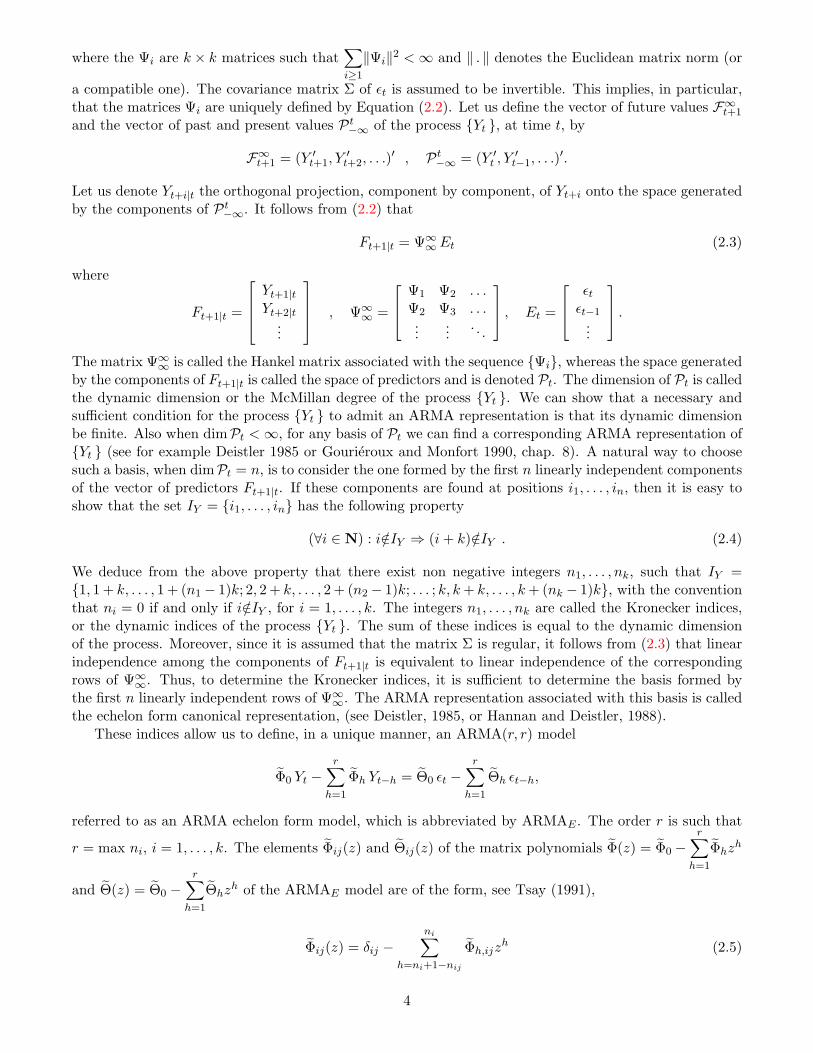
where the Ψi are k × k matrices such that∑i≥1

‖Ψi‖2 < ∞ and ‖ . ‖ denotes the Euclidean matrix norm (or

a compatible one). The covariance matrix Σ of εt is assumed to be invertible. This implies, in particular,that the matrices Ψi are uniquely defined by Equation (2.2). Let us define the vector of future values F∞

t+1

and the vector of past and present values Pt−∞ of the process {Yt }, at time t, by

F∞t+1 = (Y ′

t+1, Y′t+2, . . .)

′ , Pt−∞ = (Y ′

t , Y ′t−1, . . .)

′.

Let us denote Yt+i|t the orthogonal projection, component by component, of Yt+i onto the space generatedby the components of Pt

−∞. It follows from (2.2) that

Ft+1|t = Ψ∞∞ Et (2.3)

where

Ft+1|t =

Yt+1|tYt+2|t

...

, Ψ∞∞ =

Ψ1 Ψ2 . . .Ψ2 Ψ3 . . ....

.... . .

, Et =

εt

εt−1...

.

The matrix Ψ∞∞ is called the Hankel matrix associated with the sequence {Ψi}, whereas the space generated

by the components of Ft+1|t is called the space of predictors and is denoted Pt. The dimension of Pt is calledthe dynamic dimension or the McMillan degree of the process {Yt }. We can show that a necessary andsufficient condition for the process {Yt } to admit an ARMA representation is that its dynamic dimensionbe finite. Also when dimPt < ∞, for any basis of Pt we can find a corresponding ARMA representation of{Yt } (see for example Deistler 1985 or Gourieroux and Monfort 1990, chap. 8). A natural way to choosesuch a basis, when dimPt = n, is to consider the one formed by the first n linearly independent componentsof the vector of predictors Ft+1|t. If these components are found at positions i1, . . . , in, then it is easy toshow that the set IY = {i1, . . . , in} has the following property

(∀i ∈ N) : i/∈IY ⇒ (i + k)/∈IY . (2.4)

We deduce from the above property that there exist non negative integers n1, . . . , nk, such that IY ={1, 1 + k, . . . , 1 + (n1 − 1)k; 2, 2 + k, . . . , 2 + (n2 − 1)k; . . . ; k, k + k, . . . , k + (nk − 1)k}, with the conventionthat ni = 0 if and only if i/∈IY , for i = 1, . . . , k. The integers n1, . . . , nk are called the Kronecker indices,or the dynamic indices of the process {Yt }. The sum of these indices is equal to the dynamic dimensionof the process. Moreover, since it is assumed that the matrix Σ is regular, it follows from (2.3) that linearindependence among the components of Ft+1|t is equivalent to linear independence of the correspondingrows of Ψ∞

∞. Thus, to determine the Kronecker indices, it is sufficient to determine the basis formed bythe first n linearly independent rows of Ψ∞

∞. The ARMA representation associated with this basis is calledthe echelon form canonical representation, (see Deistler, 1985, or Hannan and Deistler, 1988).

These indices allow us to define, in a unique manner, an ARMA(r, r) model

Φ0 Yt −r∑

h=1

Φh Yt−h = Θ0 εt −r∑

h=1

Θh εt−h,

referred to as an ARMA echelon form model, which is abbreviated by ARMAE . The order r is such that

r = max ni, i = 1, . . . , k. The elements Φij(z) and Θij(z) of the matrix polynomials Φ(z) = Φ0 −r∑

h=1

Φhzh

and Θ(z) = Θ0 −r∑

h=1

Θhzh of the ARMAE model are of the form, see Tsay (1991),

Φij(z) = δij −ni∑

h=ni+1−nij

Φh,ijzh (2.5)

4

and

Θij(z) = δij −ni∑

h=ni+1−mij

Θh,ijzh, (2.6)

where the Φh,ij and Θh,ij are real parameters,

nij =

{min(ni + 1, nj) if j < i ,min(ni, nj) otherwise ,

and

mij =

{ni + 1 if i > j and ni < nj ,ni otherwise .

Given that Φ0 = Θ0, relation (2.6) can be equivalently written as (see Nsiri and Roy, 1992),

Θij(z) = Φ0,ij −ni∑

h=1

Θh,ijzh.

Once we know the Kronecker indices n1, . . . , nk of the process {Yt }, we can define the ARMAE model(ARMA echelon form model) by employing relations (2.5) and (2.6). The i–th equation of this model isgiven by

Φ0,i.Yt −ni∑

h=1

Φh,i.Yt−h = Θ0,i.εt −ni∑

h=1

Θh,i.εt−h (2.7)

where Φh,i. and Θh,i. respectively denote the i–th row of the matrices Φh and Θh. The relation (2.7) canbe written in the “refined” form

Φ0,i.Yt −pi∑

h=1

Φh,i.Yt−h = Θ0,i.εt −qi∑

h=1

Θh,i.εt−h,

where pi and qi are such that Φpi,i. 6= 0 and Θqi,i. 6= 0, and thus we have max (pi, qi) = ni.The echelon form structure leads to

(Φ0 −p∑

j=1

ΦjBj)Yt = (Θ0 −

q∑j=1

ΘjBj)εt, (2.8)

where Φ0 = Θ0 is a lower triangular matrix with 1’s along the main diagonal. In addition, when a refinedARMA echelon form is obtained, there are some linear constraints, generally that some coefficients areequal to zero, thereby reducing the number of parameters that need to be estimated. Note that (2.8) canbe transformed in (2.1), by letting Φj = Φ−1

0 Φj , j = 1, ..., p, Θh = Φ−10 Θh, h = 1, ..., q.

2.2 The scalar component model

Another way to write down a canonical form is given by the so-called scalar component model (SCM)approach. Let us consider a VARMA(p, q) process satisfying (2.1). A linear combination X

(1)t = v′1Yt

follows a SCM(p1,q1) model where p1 ≤ p and q1 ≤ q, if v′1Φp1 6= 0, v′1Φj = 0 for j = p1 + 1, ..., p, andv′1Θq1 6= 0, v′1Θj = 0 for j = q1 + 1, ..., q. Hence

v′1Yt −p1∑

j=1

v′1ΦjYt−j = v′1εt −q1∑

j=1

v′1Θjεt−j .

5

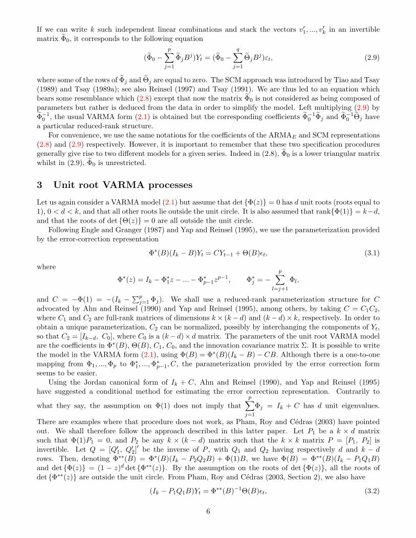
If we can write k such independent linear combinations and stack the vectors v′1, ..., v′k in an invertible

matrix Φ0, it corresponds to the following equation

(Φ0 −p∑

j=1

ΦjBj)Yt = (Φ0 −

q∑j=1

ΘjBj)εt, (2.9)

where some of the rows of Φj and Θj are equal to zero. The SCM approach was introduced by Tiao and Tsay(1989) and Tsay (1989a); see also Reinsel (1997) and Tsay (1991). We are thus led to an equation whichbears some resemblance which (2.8) except that now the matrix Φ0 is not considered as being composed ofparameters but rather is deduced from the data in order to simplify the model. Left multiplying (2.9) byΦ−1

0 , the usual VARMA form (2.1) is obtained but the corresponding coefficients Φ−10 Φj and Φ−1

0 Θj havea particular reduced-rank structure.

For convenience, we use the same notations for the coefficients of the ARMAE and SCM representations(2.8) and (2.9) respectively. However, it is important to remember that these two specification proceduresgenerally give rise to two different models for a given series. Indeed in (2.8), Φ0 is a lower triangular matrixwhilst in (2.9), Φ0 is unrestricted.

3 Unit root VARMA processes

Let us again consider a VARMA model (2.1) but assume that det {Φ(z)} = 0 has d unit roots (roots equal to1), 0 < d < k, and that all other roots lie outside the unit circle. It is also assumed that rank{Φ(1)} = k−d,and that the roots of det {Θ(z)} = 0 are all outside the unit circle.

Following Engle and Granger (1987) and Yap and Reinsel (1995), we use the parameterization providedby the error-correction representation

Φ∗(B)(Ik −B)Yt = CYt−1 + Θ(B)εt, (3.1)

where

Φ∗(z) = Ik − Φ∗1z − ...− Φ∗

p−1zp−1, Φ∗

j = −p∑

l=j+1

Φl,

and C = −Φ(1) = −(Ik −∑p

j=1 Φj). We shall use a reduced-rank parameterization structure for Cadvocated by Ahn and Reinsel (1990) and Yap and Reinsel (1995), among others, by taking C = C1C2,where C1 and C2 are full-rank matrices of dimensions k× (k− d) and (k− d)× k, respectively. In order toobtain a unique parameterization, C2 can be normalized, possibly by interchanging the components of Yt,so that C2 = [Ik−d, C0], where C0 is a (k− d)× d matrix. The parameters of the unit root VARMA modelare the coefficients in Φ∗(B), Θ(B), C1, C0, and the innovation covariance matrix Σ. It is possible to writethe model in the VARMA form (2.1), using Φ(B) = Φ∗(B)(Ik −B)− CB. Although there is a one-to-onemapping from Φ1, ...,Φp to Φ∗

1, ...,Φ∗p−1, C, the parameterization provided by the error correction form

seems to be easier.Using the Jordan canonical form of Ik + C, Ahn and Reinsel (1990), and Yap and Reinsel (1995)

have suggested a conditional method for estimating the error correction representation. Contrarily to

what they say, the assumption on Φ(1) does not imply thatp∑

j=1

Φj = Ik + C has d unit eigenvalues.

There are examples where that procedure does not work, as Pham, Roy and Cedras (2003) have pointedout. We shall therefore follow the approach described in this latter paper. Let P1 be a k × d matrixsuch that Φ(1)P1 = 0, and P2 be any k × (k − d) matrix such that the k × k matrix P = [P1, P2] isinvertible. Let Q = [Q′

1, Q′2]′ be the inverse of P , with Q1 and Q2 having respectively d and k − d

rows. Then, denoting Φ∗∗(B) = Φ∗(B)(Ik − P2Q2B) + Φ(1)B, we have Φ(B) = Φ∗∗(B)(Ik − P1Q1B)and det {Φ(z)} = (1 − z)d det {Φ∗∗(z)}. By the assumption on the roots of det {Φ(z)}, all the roots ofdet {Φ∗∗(z)} are outside the unit circle. From Pham, Roy and Cedras (2003, Section 2), we also have

(Ik − P1Q1B)Yt = Φ∗∗(B)−1Θ(B)εt, (3.2)

6

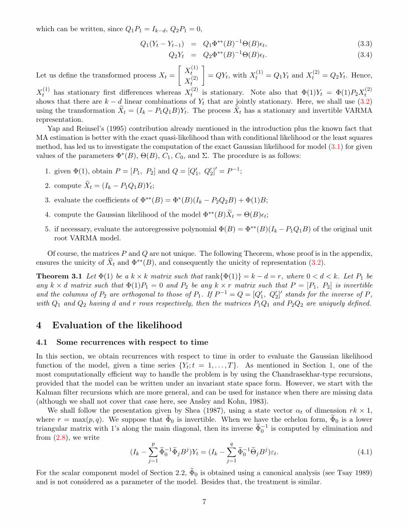
which can be written, since Q1P1 = Ik−d, Q2P1 = 0,

Q1(Yt − Yt−1) = Q1Φ∗∗(B)−1Θ(B)εt, (3.3)Q2Yt = Q2Φ∗∗(B)−1Θ(B)εt. (3.4)

Let us define the transformed process Xt =

[X

(1)t

X(2)t

]= QYt, with X

(1)t = Q1Yt and X

(2)t = Q2Yt. Hence,

X(1)t has stationary first differences whereas X

(2)t is stationary. Note also that Φ(1)Yt = Φ(1)P2X

(2)t

shows that there are k − d linear combinations of Yt that are jointly stationary. Here, we shall use (3.2)using the transformation Xt = (Ik − P1Q1B)Yt. The process Xt has a stationary and invertible VARMArepresentation.

Yap and Reinsel’s (1995) contribution already mentioned in the introduction plus the known fact thatMA estimation is better with the exact quasi-likelihood than with conditional likelihood or the least squaresmethod, has led us to investigate the computation of the exact Gaussian likelihood for model (3.1) for givenvalues of the parameters Φ∗(B), Θ(B), C1, C0, and Σ. The procedure is as follows:

1. given Φ(1), obtain P = [P1, P2] and Q = [Q′1, Q′

2]′ = P−1;

2. compute Xt = (Ik − P1Q1B)Yt;

3. evaluate the coefficients of Φ∗∗(B) = Φ∗(B)(Ik − P2Q2B) + Φ(1)B;

4. compute the Gaussian likelihood of the model Φ∗∗(B)Xt = Θ(B)εt;

5. if necessary, evaluate the autoregressive polynomial Φ(B) = Φ∗∗(B)(Ik−P1Q1B) of the original unitroot VARMA model.

Of course, the matrices P and Q are not unique. The following Theorem, whose proof is in the appendix,ensures the unicity of Xt and Φ∗∗(B), and consequently the unicity of representation (3.2).

Theorem 3.1 Let Φ(1) be a k × k matrix such that rank{Φ(1)} = k − d = r, where 0 < d < k. Let P1 beany k × d matrix such that Φ(1)P1 = 0 and P2 be any k × r matrix such that P = [P1, P2] is invertibleand the columns of P2 are orthogonal to those of P1. If P−1 = Q = [Q′

1, Q′2]′ stands for the inverse of P ,

with Q1 and Q2 having d and r rows respectively, then the matrices P1Q1 and P2Q2 are uniquely defined.

4 Evaluation of the likelihood

4.1 Some recurrences with respect to time

In this section, we obtain recurrences with respect to time in order to evaluate the Gaussian likelihoodfunction of the model, given a time series {Yt; t = 1, . . . , T}. As mentioned in Section 1, one of themost computationally efficient way to handle the problem is by using the Chandrasekhar-type recursions,provided that the model can be written under an invariant state space form. However, we start with theKalman filter recursions which are more general, and can be used for instance when there are missing data(although we shall not cover that case here, see Ansley and Kohn, 1983).

We shall follow the presentation given by Shea (1987), using a state vector αt of dimension rk × 1,where r = max(p, q). We suppose that Φ0 is invertible. When we have the echelon form, Φ0 is a lowertriangular matrix with 1’s along the main diagonal, then its inverse Φ−1

0 is computed by elimination andfrom (2.8), we write

(Ik −p∑

j=1

Φ−10 ΦjB

j)Yt = (Ik −q∑

j=1

Φ−10 ΘjB

j)εt. (4.1)

For the scalar component model of Section 2.2, Φ0 is obtained using a canonical analysis (see Tsay 1989)and is not considered as a parameter of the model. Besides that, the treatment is similar.

7

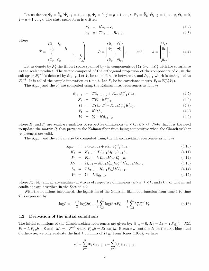
Let us denote Φj = Φ−10 Φj , j = 1, . . . , p, Φj = 0, j = p + 1, . . . , r, Θj = Φ−1

0 Θj , j = 1, . . . , q, Θj = 0,j = q + 1, . . . , r. The state space form is written

Yt = h′αt + εt (4.2)αt = Tαt−1 + Rεt−1, (4.3)

where

T =

Φ1 Ik

Φ2 Ik...

. . . Ik

Φr 0k · · · 0k

, R =

Φ1 −Θ1

Φ2 −Θ2...

Φr −Θr

, and h =

Ik

0k...

0k

. (4.4)

Let us denote by F t1 the Hilbert space spanned by the components of {Y1, Y2, ..., Yt} with the covariance

as the scalar product. The vector composed of the orthogonal projection of the components of αt in thesub-space F t−1

1 is denoted by αt|t−1. Let Vt be the difference between αt and αt|t−1 which is orthogonal toF t−1

1 . It is called the sample innovation at time t. Let Ft be its covariance matrix Ft = E(VtV′t ).

The αt|t−1 and the Ft are computed using the Kalman filter recurrences as follows

αt|t−1 = T αt−1|t−2 + Kt−1F−1t−1Vt−1, (4.5)

Kt = TPt−1hF−1t−1, (4.6)

Pt = TPt−1T′ + Kt−1F

−1t−1K

′t−1, (4.7)

Ft = h′Pth, (4.8)Vt = Yt − h′αt|t−1, (4.9)

where Kt and Pt are auxiliary matrices of respective dimensions rk × k, rk × rk. Note that it is the needto update the matrix Pt that prevents the Kalman filter from being competitive when the Chandrasekharrecurrences are valid.

The αt|t−1 and the Ft can also be computed using the Chandrasekhar recurrences as follows

αt|t−1 = T αt−1|t−2 + Kt−1F−1t−1Vt−1, (4.10)

Kt = Kt−1 + TLt−1Mt−1L′t−1h, (4.11)

Ft = Ft−1 + h′Lt−1Mt−1L′t−1h, (4.12)

Mt = Mt−1 −Mt−1L′t−1hF−1

t h′Lt−1Mt−1, (4.13)Lt = TLt−1 −Kt−1F

−1t−1h

′Lt−1, (4.14)Vt = Yt − h′αt|t−1, (4.15)

where Kt, Mt, and Lt are auxiliary matrices of respective dimensions rk× k, k× k, and rk× k. The initialconditions are described in the Section 4.2.

With the notations introduced, the logarithm of the Gaussian likelihood function from time 1 to timeT is expressed by

logL = −Tk

2log(2π)− 1

2

T∑t=1

log(detFt)−12

T∑t=1

V ′t F−1

t Vt. (4.16)

4.2 Derivation of the initial conditions

The initial conditions of the Chandrasekhar recurrences are given by: α1|0 = 0, K1 = L1 = TP1|0h + RΣ,F1 = h′P1|0h + Σ and M1 = −F−1

1 where P1|0h = E(αtα′t)h. Because h contains Ik on the first block and

0 otherwise, we only evaluate the first k columns of P1|0. From Jones (1980), we have

αit =

p∑j=i

ΦjYt+i−j−1 −q∑

j=i

Θjεt+i−j−1,

8

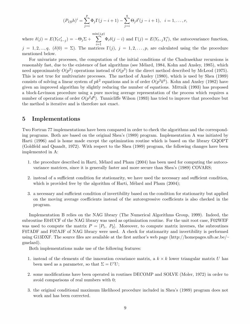
(P1|0h)i =p∑

j=i

ΦjΓ(j − i + 1)−q∑

j=i

Θjδ′(j − i + 1), i = 1, . . . , r,

where δ(j) = E(Ytε′t−j) = −ΘjΣ +

min(j,p)∑i=1

Φiδ(j − i) and Γ(j) = E(Yt−jY′t ), the autocovariance function,

j = 1, 2, ..., q, (δ(0) = Σ). The matrices Γ(j), j = 1, 2, . . . , p, are calculated using the the procedurementioned below.

For univariate processes, the computation of the initial conditions of the Chadrasekhar recursions isreasonably fast, due to the existence of fast algorithms (see Melard, 1984, Kohn and Ansley, 1985), whichneed approximately O(p2) operations instead of O(p3) for the direct method described by McLeod (1975).This is not true for multivariate processes. The method of Ansley (1980), which is used by Shea (1989)consists of solving a linear system of pk2 equations and is of order O(p3k6). Kohn and Ansley (1982) havegiven an improved algorithm by slightly reducing the number of equations. Mittnik (1993) has proposeda block-Levinson procedure using a pure moving average representation of the process which requires anumber of operations of order O(p2d6). Tunnicliffe Wilson (1993) has tried to improve that procedure butthe method is iterative and is therefore not exact.

5 Implementations

Two Fortran 77 implementations have been compared in order to check the algorithms and the correspond-ing programs. Both are based on the original Shea’s (1989) program. Implementation A was initiated byHarti (1996) and is home made except the optimization routine which is based on the library GQOPT(Goldfeld and Quandt, 1972). With respect to the Shea (1989) program, the following changes have beenimplemented in A:

1. the procedure described in Harti, Melard and Pham (2004) has been used for computing the autoco-variance matrices, since it is generally faster and more secure than Shea’s (1989) COVARS;

2. instead of a sufficient condition for stationarity, we have used the necessary and sufficient condition,which is provided free by the algorithm of Harti, Melard and Pham (2004);

3. a necessary and sufficient condition of invertibility based on the condition for stationarity but appliedon the moving average coefficients instead of the autoregressive coefficients is also checked in theprogram.

Implementation B relies on the NAG library (The Numerical Algorithms Group, 1999). Indeed, thesubroutine E04UCF of the NAG library was used as optimization routine. For the unit root case, F02WEFwas used to compute the matrix P = [P1, P2]. Moreover, to compute matrix inverses, the subroutinesF07ADF and F07AJF of NAG library were used. A check for stationarity and invertibility is performedusing G13DXF. The source files are available at the first author’s web page (http://homepages.ulb.ac.be/˜gmelard).

Both implementations make use of the following features:

1. instead of the elements of the innovation covariance matrix, a k × k lower triangular matrix U hasbeen used as a parameter, so that Σ = U ′U ;

2. some modifications have been operated in routines DECOMP and SOLVE (Moler, 1972) in order toavoid comparisons of real numbers with 0;

3. the original conditional maximum likelihood procedure included in Shea’s (1989) program does notwork and has been corrected.

9

The empirical results presented here were obtained using implementation B but those of implementationA are very close. The simulations described in Section 7 were produced using implementation B. For ourvector of parameters, the optimization procedure gives the observed Fisher information (or Hessian) matrixof the estimators. Their estimated standard errors are computed by inverting the observed Hessian matrixat the final estimate of the parameters.

6 Empirical comparisons

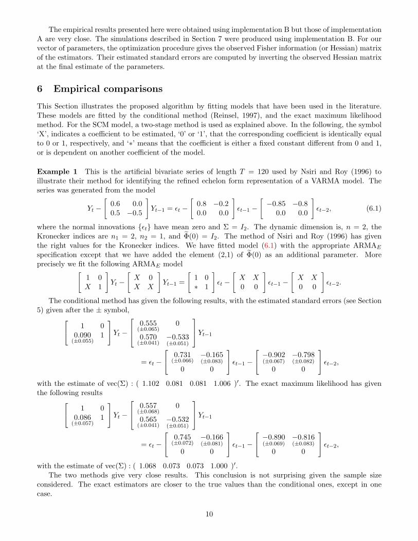
This Section illustrates the proposed algorithm by fitting models that have been used in the literature.These models are fitted by the conditional method (Reinsel, 1997), and the exact maximum likelihoodmethod. For the SCM model, a two-stage method is used as explained above. In the following, the symbol‘X’, indicates a coefficient to be estimated, ‘0’ or ‘1’, that the corresponding coefficient is identically equalto 0 or 1, respectively, and ‘∗’ means that the coefficient is either a fixed constant different from 0 and 1,or is dependent on another coefficient of the model.

Example 1 This is the artificial bivariate series of length T = 120 used by Nsiri and Roy (1996) toillustrate their method for identifying the refined echelon form representation of a VARMA model. Theseries was generated from the model

Yt −[

0.6 0.00.5 −0.5

]Yt−1 = εt −

[0.8 −0.20.0 0.0

]εt−1 −

[−0.85 −0.8

0.0 0.0

]εt−2, (6.1)

where the normal innovations {εt} have mean zero and Σ = I2. The dynamic dimension is, n = 2, theKronecker indices are n1 = 2, n2 = 1, and Φ(0) = I2. The method of Nsiri and Roy (1996) has giventhe right values for the Kronecker indices. We have fitted model (6.1) with the appropriate ARMAE

specification except that we have added the element (2,1) of Φ(0) as an additional parameter. Moreprecisely we fit the following ARMAE model[

1 0X 1

]Yt −

[X 0X X

]Yt−1 =

[1 0∗ 1

]εt −

[X X0 0

]εt−1 −

[X X0 0

]εt−2.

The conditional method has given the following results, with the estimated standard errors (see Section5) given after the ± symbol, 1 0

0.090(±0.055)

1

Yt −

0.555(±0.065)

0

0.570(±0.041)

−0.533(±0.051)

Yt−1

= εt −

0.731(±0.066)

−0.165(±0.083)

0 0

εt−1 −

−0.902(±0.067)

−0.798(±0.082)

0 0

εt−2,

with the estimate of vec(Σ) : ( 1.102 0.081 0.081 1.006 )′. The exact maximum likelihood has giventhe following results 1 0

0.086(±0.057)

1

Yt −

0.557(±0.068)

0

0.565(±0.041)

−0.532(±0.051)

Yt−1

= εt −

0.745(±0.072)

−0.166(±0.081)

0 0

εt−1 −

−0.890(±0.069)

−0.816(±0.083)

0 0

εt−2,

with the estimate of vec(Σ) : ( 1.068 0.073 0.073 1.000 )′.The two methods give very close results. This conclusion is not surprising given the sample size

considered. The exact estimators are closer to the true values than the conditional ones, except in onecase.

10

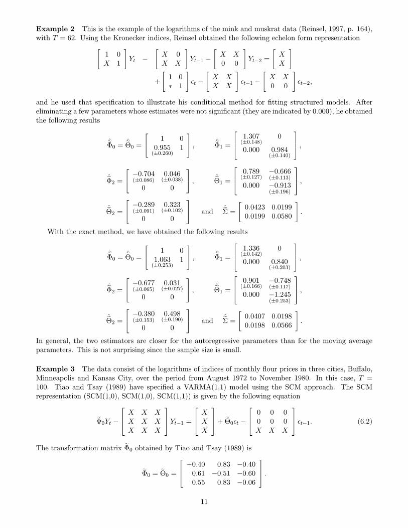
Example 2 This is the example of the logarithms of the mink and muskrat data (Reinsel, 1997, p. 164),with T = 62. Using the Kronecker indices, Reinsel obtained the following echelon form representation[

1 0X 1

]Yt −

[X 0X X

]Yt−1 −

[X X0 0

]Yt−2 =

[XX

]

+

[1 0∗ 1

]εt −

[X XX X

]εt−1 −

[X X0 0

]εt−2,

and he used that specification to illustrate his conditional method for fitting structured models. Aftereliminating a few parameters whose estimates were not significant (they are indicated by 0.000), he obtainedthe following results

ˆΦ0 = ˆΘ0 =

1 00.955

(±0.260)1

,ˆΦ1 =

1.307(±0.148)

0

0.000 0.984(±0.140)

,

ˆΦ2 =

−0.704(±0.086)

0.046(±0.038)

0 0

,ˆΘ1 =

0.789(±0.127)

−0.666(±0.113)

0.000 −0.913(±0.196)

,

ˆΘ2 =

−0.289(±0.091)

0.323(±0.102)

0 0

and ˆΣ =

[0.0423 0.01990.0199 0.0580

].

With the exact method, we have obtained the following results

ˆΦ0 = ˆΘ0 =

1 01.063

(±0.253)1

,ˆΦ1 =

1.336(±0.142)

0

0.000 0.840(±0.203)

,

ˆΦ2 =

−0.677(±0.065)

0.031(±0.027)

0 0

,ˆΘ1 =

0.901(±0.166)

−0.748(±0.117)

0.000 −1.245(±0.253)

,

ˆΘ2 =

−0.380(±0.153)

0.498(±0.190)

0 0

and ˆΣ =

[0.0407 0.01980.0198 0.0566

].

In general, the two estimators are closer for the autoregressive parameters than for the moving averageparameters. This is not surprising since the sample size is small.

Example 3 The data consist of the logarithms of indices of monthly flour prices in three cities, Buffalo,Minneapolis and Kansas City, over the period from August 1972 to November 1980. In this case, T =100. Tiao and Tsay (1989) have specified a VARMA(1,1) model using the SCM approach. The SCMrepresentation (SCM(1,0), SCM(1,0), SCM(1,1)) is given by the following equation

Φ0Yt −

X X XX X XX X X

Yt−1 =

XXX

+ Θ0εt −

0 0 00 0 0X X X

εt−1. (6.2)

The transformation matrix Φ0 obtained by Tiao and Tsay (1989) is

Φ0 = Θ0 =

−0.40 0.83 −0.400.61 −0.51 −0.600.55 0.83 −0.06

.

11

Probably because the package which they used for model fitting did not cope with the presence of Φ0,they used a two-stage approach. More precisely, after the computation of the matrix Φ0 and given thatthe transformation Xt = Φ0Yt does not alter the parameter specification, they fitted the model for thetransformed series Xt. Replacing in their results Xt by Φ0Yt, we obtain −0.40 0.83 −0.40

0.61 −0.51 −0.600.55 0.83 −0.06

Yt −

−0.364 0.741 −0.3400.531 −0.271 −0.7220.774 0.136 0.352

Yt−1 =

−0.02−0.16

0.26

+

−0.40 0.83 −0.400.61 −0.51 −0.600.55 0.83 −0.06

εt −

0 0 00 0 0

1.518 −1.332 −0.069

εt−1.

Using the exact method of this paper, we obtain the following fitted model −0.40 0.83 −0.400.61 −0.51 −0.600.55 0.83 −0.06

Yt −

−0.362 0.738 −0.3450.494 −0.235 −0.7330.825 0.075 0.374

Yt−1 =

−0.007−0.124

0.215

+

−0.40 0.83 −0.400.61 −0.51 −0.600.55 0.83 −0.06

εt −

0 0 00 0 0

1.421 −1.256 −0.062

εt−1.

The results are close but not identical because the so-called exact estimation method of SCA (Lui and Hu-dak, 1986) computes, in fact, the exact likelihood for an autoregressive model, not for an ARMA model.

Example 4 We consider the bivariate time series of seasonally adjusted monthly U.S. housing dataconsisting of housing starts and housing sold during the period from 1965 to 1974 (Hilmer and Tiao, 1979),with T = 120. The error correction form model specified by Reinsel (1997, p. 206) is

(1−B)Yt =

[XX

] [1 X

]Yt−1 + εt (6.3)

and he obtained the following estimates

C1 =

[−0.523

0.141

], C2 =

[1 −1.872

], Σ =

[26.59 5.975.97 9.87

].

The model fitted by the exact (conditionally on the first observation) Gaussian maximum likelihood methodgives the following results

C1 =

−0.517(±0.082)

0.142(±0.048)

, C2 =[

1 −1.872(±0.086)

], Σ =

[26.69 6.036.03 9.87

].

This is not surprising because the two methods are generally close for estimating pure VAR models evenif the sample size is small.

Example 5 The data consists of the quarterly AAA corporate bonds and commercial paper series from1953 to 1970 (Haugh and Box, 1977; Reinsel, 1997, p. 306), where T = 72. The model specified in errorcorrection form by Reinsel (1997, p. 213) is

(1−B)Yt =

[XX

] [1 X

]Yt−1 +

[X XX X

](1−B)Yt−1 +

[X XX X

](1−B)Yt−2 + εt.

12

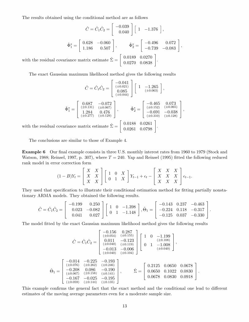
The results obtained using the conditional method are as follows

C = C1C2 =

[−0.039

0.040

] [1 −1.376

],

Φ∗1 =

[0.628 −0.0601.186 0.507

], Φ∗

2 =

[−0.496 0.072−0.739 −0.083

],

with the residual covariance matrix estimate Σ =

[0.0189 0.02700.0270 0.0838

].

The exact Gaussian maximum likelihood method gives the following results

C = C1C2 =

−0.041(±0.021)

0.085(±0.044)

[1 −1.265

(±0.063)

],

Φ∗1 =

0.687(±0.131)

−0.072(±0.067)

1.284(±0.277)

0.476(±0.129)

, Φ∗2 =

−0.465(±0.152)

0.073(±0.065)

−0.691(±0.310)

−0.038(±0.128)

,

with the residual covariance matrix estimate Σ =

[0.0188 0.02610.0261 0.0798

].

The conclusions are similar to those of Example 4.

Example 6 Our final example consists in three U.S. monthly interest rates from 1960 to 1979 (Stock andWatson, 1988; Reinsel, 1997, p. 307), where T = 240. Yap and Reinsel (1995) fitted the following reducedrank model in error correction form

(1−B)Yt =

X XX XX X

[1 0 X0 1 X

]Yt−1 + εt −

X X XX X XX X X

εt−1.

They used that specification to illustrate their conditional estimation method for fitting partially nonsta-tionary ARMA models. They obtained the following results.

C = C1C2 =

−0.199 0.2500.023 −0.0820.041 0.027

[1 0 −1.3980 1 −1.148

], Θ1 =

−0.143 0.237 −0.463−0.224 0.118 −0.317−0.125 0.037 −0.330

.

The model fitted by the exact Gaussian maximum likelihood method gives the following results

C = C1C2 =

−0.156(±0.054)

0.287(±0.155)

0.011(±0.040)

−0.123(±0.119)

−0.013(±0.040)

−0.006(±0.104)

1 0 −1.199

(±0.108)

0 1 −1.008(±0.040)

,

Θ1 =

−0.014(±0.076)

−0.225(±0.262)

−0.193(±0.246)

−0.208(±0.067)

0.086(±0.158)

−0.190(±0.141)

−0.167(±0.059)

−0.025(±0.144)

−0.195(±0.135)

, Σ =

0.2125 0.0650 0.06780.0650 0.1022 0.08300.0678 0.0830 0.0918

.

This example confirms the general fact that the exact method and the conditional one lead to differentestimates of the moving average parameters even for a moderate sample size.

13

7 Some Monte Carlo results

In this Monte Carlo study, we mainly investigate the finite sample properties of both the conditionalmethod and the Gaussian exact maximum likelihood method. We compare their performances and wecheck the adequacy of their standard errors. In order to do that, we realized two different experimentsto illustrate the results in each of the two cases: ARMA echelon and unit root models. The standardARMA case was omitted because it was widely studied by Shea (1989). In the first experiment we considera bivariate ARMAE(1,4) model that satisfies both the stationarity and invertibility conditions. In thesecond experiment we consider a trivariate partially non-stationary ARMA(1,4) model with one unit root(d =1). The two series lengths considered were 50 and 100. For each of these two experiments and for eachof the two series lengths, the G05HDF subroutine of the NAG library (NAG, 1995) was used to generateGaussian series from the corresponding standard VARMA data generating process (Barone, 1987, and Shea,1988). Then, suitable transformations were applied to obtain the series from the non standard VARMAprocesses, For each replication, the two estimation methods (exact and conditional) were performed usingthe implementations of Section 5.

In order to perform a valid comparison, for both experiments, we kept only the first 100 replicationsfor which

(i) the optimization procedure E04UCF of the NAG library reaches an optimal solution for both methods(conditional and exact), i.e. E04UCF ended without error indicators or warnings for both methods;

(ii) for both methods, the optimal solution obtained satisfies the stationarity and invertibility conditions.

Moreover, to insure that initial values of the parameters do not affect our conclusions, those values forboth methods were taken equal to the true parameter values.

For each parameter, the following results are reported:

(1) MEAN: the average of the estimates over the replications;

(2) OSD: the Observed Standard Deviation that is defined as the square root of the average over thereplications of the variances obtained by the optimization procedure;

(3) ESD: the Empirical Standard Deviation across the replications.

7.1 Experiment 1

In the first experiment, we generate data from the following ARMAE model

Yt −[

0.9 0.00.2 0.9

]Yt−1 = εt −

[0.0 0.00.0 0.1

]εt−3 −

[0.9 −0.80.0 0.0

]εt−4,

where the innovations {εt} have mean zero and Σ = I2. The main purpose is to fit the following ARMAE

model [1 0X 1

]Yt −

[X 0X X

]Yt−1 =

[1 0∗ 1

]εt −

[0 00 X

]εt−3 −

[X X0 0

]εt−4, (7.1)

for each replication. Of course, the (2, 1)-element of Φ0 is a parameter in the model. The results arereported in Table 1. The latter is presented as a 3×1 block matrix, the first block gives the true parametervalues and the second and third ones present the results of the two estimation methods (conditional andexact) for the sample sizes 50 and 100 respectively. For each estimated coefficient, we provide the MEAN,OSD and ESD based on 100 independent realizations. For the coefficients that are not estimated such asthe elements of Φ0 except (2,1), or the element (1,2) of Φ1 and some elements in Θ3, and Θ4, the MEANcorresponds to the true value and we put a dash for the OSD and ESD. The lower triangular matrix Ubeing estimated instead of Σ, we provide the results for the elements of U . Since Σ = I2 in this model, the

14

true U is also equal to I2. The OSD and ESD are presented only for the lower part of U . To underlinethe differences between the two methods, the conditional and exact estimates averages that are far apartor far from the true value were put in bold.

Inspection of Table 1 reveals that, for both sample sizes, the averages obtained from the exact methodare closer to the true values than those obtained by the conditional method. The greatess differencesbetween the two methods appear for the (1, 1)-element of Θ4 and the (2, 1)-element of Θ3. The conditionalmethod is particularly inefficient for estimating Θ4. Note that for both methods, as the sample sizeincreases, the averages become closer to the true values. Moreover, for the series length T = 100, thebias of the exact estimates are smaller than those of the conditional ones. Note also that for the largersample size (T = 100), the OSD and ESD are close for all parameters. However, with T = 50, for a fewparameters, the OSD and ESD differ when the exact method is performed. Experiments for other samplesizes were considered but the results are not reported. They indicate that the OSD and ESD are muchcloser as the sample size increases.

The true model

Φ0 Φ1 Θ3 Θ4 U1 0 .900 0 0 0 .900 -.800 1.000 0

.000 1 .200 .900 0 .100 0 0 .000 1.000The estimated model

Size Method Φ0 Φ1 Θ3 Θ4 U

50 COND MEAN 1 0 .858 0 0 0 .640 -.746 1.166 0-.057 1 .173 .880 0 .078 —- —- .094 1.054

OSD —- —- .065 —- —- —- .134 .149 .116 0.159 —- .140 .043 —- .125 —- —- .155 .106

ESD —- —- .075 0 —- —- .166 .194 .168 —-.127 —- .111 .044 —- .136 —- —- .246 .192

EXACT MEAN 1 0 .874 0 0 0 .813 -.854 .998 0-.057 1 .171 .883 0 .108 —- —- -.009 .927

OSD —- —- .056 —- —- —- .233 .150 .130 0.117 —- .105 .035 —- .127 —- —- .154 .098

ESD —- —- .065 0 —- —- .141 .145 .120 —-.119 —- .106 .040 —- .141 —- —- .167 .010

100 COND MEAN 1 0 .880 0 0 0 .741 -.775 1.112 0-.020 1 .190 .891 0 .085 —- —- .059 1.050

OSD —- —- .039 —- —- —- .082 .086 .076 0.089 —- .080 .023 —- .075 —- —- .105 .074

ESD —- —- .040 0 —- —- .119 .117 .092 —-.079 —- .069 .025 —- .080 —- —- .143 .133

EXACT MEAN 1 0 .887 0 0 0 .900 -.825 .990 0-.019 1 .189 .893 0 .102 —- —- -.004 .983

OSD —- —- .035 —- —- —- .116 .078 .077 0.073 —- .063 .019 —- .073 —- —- .107 .071

ESD —- —- .034 0 —- —- .062 .077 .063 —-.069 —- .064 .022 —- .067 —- —- .106 .072

Table 1. Comparison of the conditional (COND) and EXACT likelihood estimation methods forthe bivariate ARMA echelon model (7.1) based on 100 replications for each of the two sample sizes.For each estimated parameter, we report the mean of the 100 estimates (MEAN), the observedstandard deviation (OSD) and the empirical standard deviation (ESD).

7.2 Experiment 2

In this experiment, we generate data from a partially non-stationary ARMA(1,4) model with one unit root

Yt −

0.602 0.433 0.1100.121 0.660 0.0660.103 0.166 0.838

Yt−1 = εt −

0.6 0 0.20 0.9 0

−0.4 −0.4 0.8

εt−4,

15

where the innovations {εt} have zero mean and

Σ =

1.0 0.5 0.40.5 1.0 0.70.4 0.7 1.0

, so U =

1 0 00.5 0.866 00.4 0.577 0.712

.

The true modelC1 C0 Θ4 U

-.398 .433 -.800 .600 0 .200 1.000 0 0.121 -.340 -.480 0 .900 0 .500 .897 0.103 .166 -.400 -.400 .800 .400 .577 .712

The estimated model

Size Method C1 C0 Θ4 U

50 COND MEAN -.430 .411 -.811 .573 0 .172 .992 0 0.119 -.430 -.488 0 .742 0 .548 .897 0.157 .131 -.411 -.091 .432 .367 .454 .816

OSD .109 .133 .217 .122 —- .116 .103 —- —-.112 .141 .134 —- .088 —- .145 .090 —-.114 .138 .149 .162 .140 .147 .132 .080

ESD .138 .169 .231 .136 —- .134 .096 —- —-.162 .177 .158 —- .099 —- .138 .110 —-.119 .144 .169 .198 .200 .171 .167 .108

EXACT MEAN -.414 .419 -.798 .587 0 .253 .957 0 0.123 -.401 -.484 0 .862 0 .510 .834 0.143 .135 -.452 -.551 .980 .394 .566 .582

OSD .101 .126 .167 .137 —- .146 .105 —- —-.100 .132 .105 —- .086 —- .136 .092 —-.105 .128 .150 .220 .254 .147 .122 .095

ESD .112 .150 .210 .147 —- .150 .097 —- —-.120 .141 .144 —- .060 —- .121 .095 —-.117 .143 .173 .228 .204 .155 .141 .092

100 COND MEAN -.409 .437 -.793 .598 0 .179 1.001 0 0.129 -.371 -.472 0 .799 0 .533 .901 0.132 .155 -.409 -.151 .520 .393 .492 .806

OSD .068 .084 .055 .068 —- .073 .071 —- —-.065 .086 .034 —- .048 —- .099 .062 —-.072 .088 .085 .096 .102 .099 .089 .053

ESD .071 .092 .053 .074 —- .079 .074 —- —-.076 .094 .039 —- .060 —- .109 .061 —-.072 .100 .101 .136 .140 .108 .100 .071

EXACT MEAN -.410 .446 -.800 .611 0 .229 .980 0 0.119 -.352 -.478 0 .894 0 .510 .854 0.122 .152 -.404 -.495 .931 .392 .585 .642

OSD .063 .079 .045 .066 —- .075 .072 —- —-.051 .071 .022 —- .035 —- .096 .063 —-.065 .082 .076 .114 .121 .101 .085 .057

ESD .065 .088 .038 .073 —- .078 .075 —- —-.059 .080 .018 —- .032 —- .103 .054 —-.072 .091 .083 .130 .145 .109 .081 .064

Table 2.Comparison of the conditional (COND) and EXACT likelihood estimation methods for the trivari-ate nonstationary ARMA(1,4) model (7.2) based on 100 replications for each of the two sample sizes. Foreach estimated parameter, we report the mean of the 100 estimates (MEAN), the observed standarddeviation (OSD) and the empirical standard deviation (ESD).

We can easily check that the matrices C1 and C0 that characterize the error-correction form are givenby

C1 =

−0.398 0.4330.121 −0.3400.103 0.166

and C0 =

[−0.80−0.48

].

16

We fit the following error-correction form model

Wt = Yt − Yt−1 =

X XX XX X

[1.0 0.0 X0.0 1.0 X

]Yt−1 + εt −

X 0 X0 X 0X X X

εt−4. (7.2)

The first observation Y0 was set equal to zero. The likelihood function is conditional on this first observation.The results are reported in Table 2 whose presentation is similar to Table 1. For each sample size andeach method, we report the average estimates of the matrices C1, C0, Θ4, and U and their respectiveOSD and ESD. The main conclusions are similar to those of Experiment 1. The exact method performsbetter than the conditional one for both sample sizes. The difference between the two methods is speciallystriking for Θ4 at both series lengths. In particular, the true value of the (3, 2)-element is −0.400 whilstthe conditional estimates averages are −0.091 at T = 50 and −0.151 at T = 100. The corresponding exactestimates averages are respectively −0.551 and −0.495.

8 Conclusions

This paper describes algorithms for exact maximum likelihood estimation of parsimonious VARMA modelsand partially nonstationary unit root VARMA. The main difference between the VARMA echelon and thestandard VARMA representation is that a triangular matrix Φ(0) is substituted to the identity matrix inthe autoregressive and moving average polynomials and that constraints of nullity are imposed to somecoefficients. The constraints do not have an impact on the likelihood function itself. However, the presenceof Φ(0) modifies the evaluation of the likelihood but the change is smaller than it could be anticipated.

Similarly, the coverage of unit root or cointegrated VARMA models for excat maximum likelihoodestimation (conditional, of course on the the first observation of the vector series) require some minorchanges in the code. In the two cases, these features are not available in the existing software packages.

We have been able to fit several models shown in the literature and to investigate in a small Monte Carlostudy the effect of the use of the exact likelihood instead of the conditional likelihood. In particular, withshort series of 50 and 100 observations, the difference between the conditional and the exact estimationscan be quite large especially for high-order moving average parameters.

There should be no problem to handle unit root VARMA models in structured form although it is notcurrently implemented. A VARMA cointegrated model in echelon form can be specified using the methodof Poskitt and Lutkepohl (1995) with Kronecker indices estimated using Bartel and Lutkepohl (1997).Another procedure for obtaining a parsimonious cointegration representation is due to Hunter and Dislis(1994).

Appendix

Proof of Theorem 3.1. The singular value decomposition of Φ(1) yields that

Φ(1) = UDV ′ = [u1, u2, ..., uk]

d1 0 0 . . . 00 d2 0 0

0 0 d3. . .

......

. . . . . . 00 0 . . . 0 dk

v′1...v′r...

v′k

,

where U and V are k × k orthogonal matrices.The null space of Φ(1), i.e., the set of vectors x such that Φ(1)x = 0, is the space generated by the

columns of the matrix G = [vr+1, ..., vk]. Now let P1 and P ∗1 be any k × d matrices such that Φ(1)P1 = 0

17

and Φ(1)P ∗1 = 0. Since P1 and P ∗

1 are full rank matrices, there exist full rank d × d matrices α and α∗

such thatP1 = Gα and P ∗

1 = Gα∗.

Hence, we haveP ∗

1 = P1α−1α∗.

In a similar way, consider k × r matrices P2 and P ∗2 such that P = [P1, P2] and P ∗ = [P ∗

1 , P ∗2 ] are

invertible, and the column vectors of P2 and P ∗2 are orthogonal to those of P1 and P ∗

1 respectively. Ofcourse, the space spanned by the column vectors of M = [v1, ..., vr] is orthogonal to the one spanned bythose of G. Hence, there exist full rank r × r matrices β and β∗ such that

P2 = Mβ and P ∗2 = Mβ∗.

Thus,P ∗

2 = P2β−1β∗.

Let Q =

[Q1

Q2

]= P−1 and Q∗ =

[Q∗

1

Q∗2

]= (P ∗)−1, we can easily check that

Q∗ =

[(α∗)−1αQ1

(β∗)−1βQ2

].

Now turning back to the product P ∗1 Q∗

1, we have that

P ∗1 Q∗

1 = P1α−1α∗(α∗)−1αQ1 = P1Q1.

In a similar way we can check that P ∗2 Q∗

2 = P2Q2, which completes the proof.

References

Aasnaes, H. B., and Kailath, T. (1973). An innovation approach to least-squares estimation - Part VII:Some applications of vector autoregressive moving average models. IEEE Transactions on AutomaticControl 18, 601-607.Ahn, S. K., and Reinsel, G. C. (1990). Estimation for partially nonstationary multivariate autoregressivemodels. Journal of the American Statistical Association 85, 813-823.Akaike, H. (1978). Covariance matrix computation of the state variable of stationary Gaussian process.Annals of the Institute of Statistical Mathematics 30, 499-504.Ansley, C. F. (1979). An algorithm for the exact likelihood of a mixed autoregressive-moving averageprocess.Biometrika 66, 59-65.Ansley, C. F. (1980). Computation of the theoretical autocovariance function for a vector ARMA pro-cess.Journal of Statistical Computation and Simulation 12, 15-24.Ansley, C. F., and Newbold, P. (1980). Finite sample properties of estimators for autoregressive-movingaverage models. Journal of Econometrics 13, 159-183.Ansley, C. F., and Kohn, R. (1983). Exact likelihood of vector autoregressive-moving average process withmissing or aggregated data. Biometrika 70, 275-278.Barone, P. (1987). A method for generating independent realization of a multivariate normal stationaryand invertible ARMA(p, q) process. Journal of Time Series Analysis 8, 125-130.Bartel, H. and Lutkepohl, H. (1997). Estimating the Kronecker indices of cointegrated echelon formVARMA models. Econometrics Journal 1, C76-C99.Brockwell, P. J., and Davis, R. A. (1987). Time Series: Theory and Methods. New York: Springer-Verlag.Caines, P. E., and Rissanen, J. (1974). Maximum likelihood estimation of parameters in multivariateGaussian stochastic processes. IEEE Transactions on Information Theory 20, 102-104.

18

Deistler M., (1985). General structure and parametrization of ARMA and state-space systems and itsrelation to statistical problems, in E.J. Hannan, P.R. Krishnaiah, M.M. Rao, Eds. Handbouk of Statistics,Vol. 5. Amesterdam: North-Holland, pp. 257-277.Demeure, C. J., and Mullis, C. T. (1989). The Euclid algorithm and the fast computation of cross-covariance and autocovariance sequences. IEEE Transactions on Acoustics, Speech, and Signal Process-ing 37, 545-552.Dufour, J. M., and Jouini, T. (2003). Asymptotic distribution of a simple linear estimator for VARMAmodels in echelon form. In Statistical Modeling and Analysis for Complex Data Problems (Duchesne, P.,and Remillard, B., Eds.). Kluwer: The Netherland. To appear.Dugre, J. P., Scharf, L. L., and Gueguen, C. (1986). Exact likelihood for stationary vector autoregressivemoving average processes. IEEE Transactions on Signal Processing 11, 105-118.Engle, R. F., and Granger, C. W. J. (1987). Co-integration and error correction: representation, estimationand testing. Econometrica 55, 251-276.Gardner, G., Harvey, A. C., and Phillips, G. D. A. (1980). An algorithm for exact maximum likelihoodestimation of autoregressive-moving average models by means of Kalman filtering. Journal of the RoyalStatistical Society C, 29, 311-322.Goldfeld, S. M., and Quandt, R. E. (1972). Nonlinear Methods in Econometrics. Amesterdam: North-HollandGourieroux, C., and Monfort, A. (1990). Series temporelles et modeles dynamiques. Paris: Economica.Hannan, E. J. (1969). The identification of vector mixed autoregressive moving average systems. Biometrika 57,223-225.Hannan, E. J., and Deistler, M. (1988), The Statistical Theory of Linear Systems. New York: Wiley.Harti M. (1996). Algorithmes pour l’estimation par pseudo-maximum de vraisemblance exacte pour desmodeles VARMA sous forme classique et sous forme structuree. Unpublished Ph.D. Thesis. Institut deStatistique et de Recherche Operationnelle, Universite Libre de Bruxelles.Harti, M., Melard, G., and Pham D. T. (2004). Computing covariances for scalar and vector ARMAprocesses. In preparation.Haugh, L. D., and Box, G. E. P. (1977). Identification of dynamic regression (distributed lag) modelsconnecting two series. Journal of the American Statistical Association 72, 121-130.Hillmer, S. C., and Tiao, G. C. (1979). Likelihood function of stationary multiple autoregressive movingaverage models. Journal of the American Statistical Association 74, 652-660.Hunter, J., and Dislis, C. (1994). A parsimonious representation and VARMA estimator for cointegration.Working paper.Jones, R. H. (1980). Maximum likelihood fitting of ARMA models to time series with missing observations.Technometrics 22, 389-395.Kohn, R., and Ansley, C. F. (1982). A note on obtaining the theoretical autocovariances of an ARMAprocess. Journal of Statistical Computation and Simulation 15, 273-283.Kohn, R., and Ansley, C. F. (1985). Computing the likelihood and its derivatives for a Gaussian ARMAmodel. Journal of Statistical Computation and Simulation 22, 229-263.Lindquist, A. (1974). A new algorithm for optimal filtering of discrete time stationary processes. SIAMJournal on Control and Optimization 12, 736-746.Lui, L.-M. and Hudak, G.B. (1986). The SCA Statistical System Analysis: Reference Manual for Fore-casting and Time series Analysis. Chicago: Scientific Computing Associates.Mauricio, J. A. (1995). Exact maximum likelihood estimation of stationary vector ARMA models. Journalof the American Statistical Association 90, 282-291.Mauricio, J. A. (1997). The exact likelihood function of stationary vector autoregressive moving averagemodel. Journal of the Royal Statistical Society C, 46, 157-171.Mauricio, J. A. (2002). An algorithm for the exact likelihood of a stationary vector autoregressive-movingaverage model. Journal of Time Series Analysis 23, 473-486.McLeod, A. I. (1975). Derivation of the theoretical autocovariance function of autoregressive-movingaverage time series. Journal of the Royal Statistical Society C, 24, 255-256.

19

Melard, G. (1984). Algorithm AS197: A fast algorithm for the exact likelihood of autoregressive-movingaverage models. Journal of the Royal Statistical Society C, 33, 104-114.Melard, G. (1985). Analyse de donnees chronologiques, Seminaire de mathematiques superieures, Seminairescientifique OTAN (NATO Advanced Study Institute), Montreal: Presses de l’Universie de Montreal.Mittnik, S. (1990). Computation of theoretical autocovariance matrices of multivariate autoregressivemoving average time series. Journal of the Royal Statistical Society B, 52, 151-155.Mittnik, S. (1991). Derivation of the unconditional state-covariance matrix for exact maximum-likelihoodestimation of ARMA models. Journal of Economic Dynamics and Control 15, 731-740.Mittnik, S. (1993). Computing theoretical autocovariances of multivariate autoregressive moving averagemodels by using a block Levinson method. Journal of the Royal Statistical Society B, 55, 435-440.Moler, C. B. (1972). Algorithm 423: Linear equation solver. Commun Association for Computing Machin-ery 15, 274.Morf, M., Sidhu, G. S., and Kailath, T. (1974). Some new alorithms for recursive estimation on constant,linear, discrete-time systems. IEEE Transactions on Automatic Control 19, 315-323.Nicholls, D. F., and Hall, A. D. (1979). The exact likelihood function of multivariate autoregressive movingaverage models. Biometrika 66, 259-264.Nsiri, S., and Roy, R. (1992). On the identification of ARMA echelon form models. Canadian Journal ofStatistics 20, 369-386.Nsiri, S., and Roy, R. (1996). Identification of refined ARMA echelon form models for multivariate timeseries. Journal of Multivariate Analysis 56, 207-231.Pearlman, J. G. (1980). An algorithm for the exact likelihood of a high-order autoregressive-moving averageprocess. Biometrika 67, 232-233.Pham, D. T., Roy R. and Cedras, L. (2003). Tests for non-correlation of two cointegrated ARMA timeseries. Journal of Time Series Analysis 24, 553-577.Poskitt, D. S. (1992). Identification of echelon canonical form for vector linear processes using least squares.Annals of Statistics 20, 195-215.Poskitt, D. S. and Lutkepohl, H. (1995). Consistent specification of cointegrated autoregressive moving-average systems. Preprint, Humbolt University, Berlin.Reinsel, G. C. (1979). FIML estimation of the dynamic simultaneous equations model with ARMA dis-turbances. Journal of Econometrics 9, 263-281.Reinsel, G. C. (1997). Elements of Multivariate Time Series Analysis, Second Edition. New York: Springer-Verlag.Rissanen, J. (1973). Algorithm for triangular decomposition of block Hankel and Toeplitz matrices withapplication to factoring positive matrix polynomials. Mathematics of Computation 27, 147-154.Rissanen, J., and Barbosa, L. (1969). Properties of infinite covariance matrices and stability of optimumpredictors. Information Sciences 1, 221-236.Schweppe, F. C. (1965). Evaluation of likelihood functions for Gaussian signals. IEEE Transactions onInformation Theory 11, 61-70.Shea, B. L. (1984). Maximum likelihood estimation of multivariate ARMA processes via the Kalman filter,in Anderson O. D., Ed, Time Series Analysis: Theory and Practice, Vol. 5. Amsterdam: North-Holland,pp. 91-101.Shea, B. L. (1987). Estimation of multivariate time series. Journal of Time Series Analysis 8, 95-109.Shea, B. L. (1988). A note on the generation of independent realisations of a vector autoregressive movingaverage process. Journal of Time Series Analysis 9, 403-410.Shea, B. L. (1989). The exact likelihood of a vector autoregressive moving average model. Journal of theRoyal Statistical Society C, 38, 161-184.Solo, V. (1984). The exact likelihood for a multivariate ARMA model. Journal of Multivariate Analysis 15,164-173.Soderstrom, T., Jezek, J. and , Kucera V. (1998). An efficient and versatile algorithm for computing thecovariance function of an ARMA process. IEEE Transactions on Signal Processing 46, 1591-1600.

20

Stock, J. C. and Watson, M. W. (1988). Testing for common trends. Journal of the American StatisticalAssociation 83, 1097-1107.The Numerical Algorithms Group (1999). Fortran 77 Library Mark 19 Manual. Oxford: NAG Ltd.Tiao, G. C., and Box, G. E. P. (1981). Modeling multiple time series with applications. Journal of theAmerican Statistical Association 76, 802-816.Tiao, G. C., and Tsay, R. S. (1989). Model specification in multivariate time series. Journal of the RoyalStatistical Society B, 51, 157-213.Tong, D. Q. (1991). Methodes d’estimation de parametres de modeles autoregressifs multivaries”. Unpub-lished Ph.D. Thesis. Universite Joseph Fourier, Grenoble.Tsay, R. S. (1989a). Identifying multivariate time series models. Journal of Time Series Analysis 10,357-372.Tsay, R. S. (1989b). Parsimonious parametrization of vector autoregressive moving average models. Jour-nal of Business and Economic Statistics 7, 327-341.Tsay, R. S. (1991). Two canonical forms for vector ARMA processes. Statistica Sinica 1, 247-269.Tunnicliffe Wilson, G. (1973). The estimation of parameters in multivariate time series models. Journalof the Royal Statistical Society B, 35, 76-85.Tunnicliffe Wilson, G. (1979). Some efficient computational procedures for high order ARMA models.Journal of Statistical Computation and Simulation bf 8, 303-309.Tunnicliffe Wilson, G. (1993). Developments in multivariate covariance generation and factorization. inSubba Rao, T., Ed., Developments in Time Series Analysis: in honor of Maurice B. Priestley. London:Chapman and Hall, pp. 26-36.Yap, S. F., and Reinsel, G. C. (1995), ”Estimation and testing for unit roots in partially nonstationaryvector autoregressive moving average models. Journal of the American Statistical Association 90, 253-267.

21