NASA Technical Memorandum 112202

Exact Integrations ofPolynomials and SymmetricQuadrature Formulas overArbitrary Polyhedral Grids

Yen Liu and Marcel Vinokur, Ames Research Center, Moffett Field, California

June 1997

National Aeronautics and

Space Administration

Ames Research CenterMoffett Field, California 94035-1000

Exact Integrations of Polynomials and Symmetric Quadrature Formulas

over Arbitrary Polyhedral Grids

Yen Liu and Marcel Vinokur

Ames Research Center

Summary

This paper is concerned with two important elements in the high-order accurate spatial discretization

of finite volume equations over arbitrary grids. One element is the inte_ation of basis functions over

arbitrary domains, which is used in expressing various spatial inte_als in terms of discrete unknowns. The

other consists of quadrature approximations to those integrals. Only polynomial basis functions applied

to polyhedral and polygonal grids are treated here. Non-triangular polygonal faces are subdivided into a

union of planar triangular facets, and the resulting triangulated polyhedron is subdivided into a union of

tetrahedra. The straight line segTnent, triangle, and tetrahedron are thus the fundamental shapes that are

the building blocks for all integrations and quadrature approximations. Integrals of products up to the fifthorder are derived in a unified manner for the three fundamental shapes in terms of the position vectors of

vertices. Results are given both in terms of tensor products and products of Cartesian coordinates. The exact

polynomial integrals are used to obtain symmetric quadrature approximations of any degree of precision up to

five for arbitrary integTals over the three fundamental domains. Using a coordinate-free formulation, simple

and rational procedures are developed to derive virtually all quadrature formulas, including some previously

unpublished. Four symmetry groups of quadrature points are introduced to derive Gauss formulas, while

their limiting forms are used to derive Lobatto formulas. Representative Gauss and Lobatto formulas are

tabulated. The relative efficiency of their application to polyhedral and polygonal grids is detailed. The

extension to higher degrees of precision is discussed.

I. Introduction

Two of the current themes in computational physics are high-order accurate methods and the employ-

ment of arbitrary grids. We are interested in using these ideas in the discretization of integral conservation

laws. As applied to a finite domain, these state that the rate of change of a conserved quantity inside a

domain is equal to integrated effects over its boundary, and possibly its net creation inside the domain. For

three-dimensional problems, the domain is a volume element, and the boundary is a closed surface. For

two-dimensional problems, the dimensions of the geometric elements are reduced by one.

A general procedure for obtaining a high-order accurate discretization of equations on a given arbitrary

grid would involve the following steps:

1. A set of basis functions is chosen to represent the solution in some local region. This region is usually

the finite conservation domain, but it could be centered with respect to part of the boundary of the con-

servation domain. The basis functions are normally chosen as polynomials, but other readily integrable

or differentiable functions can also be used.

2. A set of discrete unknowns in the neighborhood of the representation re,on is chosen to reconstruct

the local representation of the solution. These can be symmetrically located or directionally biased.

. The coefficients in the representation are evaluated in terms of the conservative unknowns. This requires

the integration of the basis functions over the conservation domain. In the most general case, a least-

squares algebraic problem with constraints must be solved.

. The boundary terms, and possible source terms, are evaluated for the conservation domain. If the bound-

ary functions are linear, and the boundary is analytically defined, the evaluation could be performed

in closed form, provided that the basis functions are integrable. In general, a high-order quadrature in

terms of point values is required. The solution at a boundary point could involve spatial derivatives

(requiring the differentiation of the basis functions) if transport terms are present. It will also generally

involve non-linear functions of the states on the two sides of the boundary.

The present paper is restricted to a discussion of two important elements in such a procedure. They are the

integration of the basis functions over arbitrary domains and quadrature approximations to general integrals

over such domains.

An arbitrary grid is defined by specifying a set of points and the lines connecting those points. For three

dimensions, the precise surfaces that form cell boundaries must also be specified. These lines and surfaces

should be defined so as to make the integration of basis functions and quadrature approximations easily

performed. (An exception could be for lines and surfaces at specified global domain boundaries, where more

complex evaluations for certain analytical shapes may be tolerated.) One therefore normally connects the

points by straight lines, although piecewise straight lines may be necessary when employing dual grids. In

two dimensions, this produces plane polygonal domains in general. For three dimensions, the finite domains

are arbitrary polyhedra, with polygonal faces of different type. For other than triangles, the faces are in

general non-planar. If the surface of a quadrilateral face is defined as a ruled surface, the integrations of

certain basis functions can be performed analytically, but the resulting expressions are extremely complex.

Also, quadrature approximations would be very difficult to obtain. It is therefore best to subdivide each

non-triangular face into a union of planar triangular facets. Efficient volume integrations can be obtained

by subdividing the resulting triangulated polyhedron into a union of tetrahedra. The face triangulations

define the shapes of the boundary surfaces, and therefore affect the answers for the surface and volume

integrations. However, once the shapes of the boundary surfaces are defined, the subdivision into tetrahedra

is just a matter of convenience in performing the volume integrations, and would not affect the final answers.

The most efficient subdivision of a polygonal face, in terms of minimizing the number of triangular facets,

can always be accomplished without introducing any additional interior points. But an efficient subdivision

of a triangulated polyhedron into tetrahedra may require the introduction of interior vertices or interior

edges. The straight line seooznent, triangle, and tetrahedron are thus the fundamental shapes that are the

building blocks for all integrations and quadrature approximations.

The simplest basis functions are polynomials, and this paper will be restricted to their integration over

the fundamental domains. Other basis functions can be more appropriate for certain classes of problems, and

will be considered in a future publication. A coordinate-free formulation using vector and tensor notation is

employed, thus simplifying the derivations, and permitting a unified presentation for the three fundamental

shapes. In this formulation, any function is expressed as a generalized Taylor series in terms of tensor products

of the position vector, whose origin can be arbitrarily defined. The integration of a general polynomial thus

involves the integration of tensor products of various order over the fundamental domains. It is possible to

express the answers for all three fundamental shapes by a unified formula for a tensor product of a given

order. Such expressions are given for products up to the fifth order, and higher-order formulas can be easily

derived by the same procedure. When the order of the tensor product is greater than the number of vertices

defining the fundamental shape, the expression is no longer unique. Some terms in the unified formulas

can then be written in terms of others. We thus obtain simplified formulas for the line segment starting

with thethirdorder,thetriangleforthefourthorder,andthetetrahedronforthefifthorder.Forpracticalapplications,expressionsforgenericmonomialsin termsof Cartesiancoordinatesarealsogiven.Fromtheseonecaneasilyobtaintheexpressionforanyspecificmonomial.

Symmetricquadratureapproximationsto integralsoverann-dimensionalsimplex,includingtrianglesandtetrahedra,havereceivedmuchattentionin recentyears.A compilationof formulasis foundin thebookby Stroud(ref. 1),with referencesto theoriginalpapersgiventherein.Someadditionalformulasarefoundin GrundmannandMSller(ref. 2). Formulas for triangles were also given by Cowper (ref. 3)

and Lyness and Jespersen (ref. 4), and for tetrahedra by Yu (ref. 5) and Keast (ref. 6). Some of the

derivations of these formulas involved algebraic methods, based on roots of orthogonal polynomials, and

were often of an ad hoc nature. Using our coordinate-free formulations, we develop very simple and rational

procedures to derive all of the above formulas, and also some useful ones that are new to our knowledge.

The exact polynomial integrals are used to obtain quadrature approximations of various degrees of precision

for arbitrary integrals over the fundamental domains. For isolated fundamental shapes, the most efficient

formulas, minimizing the number of quadrature points, are those in which the locations of the quadrature

points are unspecified. By analog-y with the one-dimensional cases, the formulas are referred as Gauss, even

for triangles and tetrahedra. For the latter two shapes, due to the non-linearity of the equations, there

may be more than one Gauss formula for a given degree of precision, and some could possess properties not

shared by the one-dimensional formulas. Quadrature points could be located outside or on the boundaries,

and some of the coefficients or weights could be negative, which may be unsuitable in some applications.

Under some conditions, it may be desirable to employ formulas that involve one or more free parameters.

While they are less efficient for isolated fundamental shapes, the parameters can be chosen so that all the

weights are positive, if this is necessary. A more important role for the free parameter(s) is to place some

or all the quadrature points on shape boundaries (vertices, edges, or faces). Such formulas are referred as

Lobatto, again by analog-y with the one-dimensional case. When the original finite domains are part of a grid

consisting of arbitrary polyhedra or polygons, these boundary elements are shared by several fundamental

shapes. Depending on the type of the polyhedra or polygons, the degree of precision, the amount of storage

available, and the parallelization of a code, a Lobatto formula may be more efficient than a Gauss formula.

We therefore present both Gauss and Lobatto formulas of various degrees of precision. Note that besides

the evaluations of boundary terms and possible source terms, quadrature approximations are useful when

calculating integrals over the conservation domain for those basis functions that are not readily integrable.

The type of term being evaluated will also play a role in choosing between a Gauss or Lobatto formula.

II. Exact Integrals of Polynomials for the Fundamental Shapes

Let r denote the position vector of a point in space with respect to an arbitrary origin. Using tensor

notation, an arbitrary function f(r) can be expanded about the origin in terms of tensor products as a

generalized Taylor series

1 1:(r) = :(0) + r- (vf)0 + 7 rr: (vv/)0 + i (vvv/)0 + .--. (i)

In our procedure for obtaining a high-order accurate discretization of equations, steps (3) and (4) require

the integration of f(r) over the conservation domain and its boundaries, in which the evaluations of the

integrals of the tensor products of r of various order over the fundamental domains are required. Let n be

the number of vertices defining the fundamental shape. The line segment (n = 2) is defined by the points

ri and r2, and has the len_h

L = Ir2 - ri[. (2a)

Similarly,thetriangle(n= 3) is defined by the points rl, r2, and r3, and has the area

1

S = _](r2- rl) x (r3 - r2)l,

and the tetrahedron (n = 4) is defined by the points rl, r2, r3, and r4, and has the volume

1

V = _J(r2 - rl) × (r3 - rl). (r4 - rl)].

(2b)

(2c)

In order to derive the formulas for the integrals of the tensor products, instead of employing the conven-

tional simplex coordinates, it is simpler for our purposes to use the independent parametric representations

for the three fundamental shapes shown in figure l(a-c). Here the parameters u, v, and w range from 0 to

1. A point on the line segznent is given by

r-- rl(1 - u) + r2u, (3a)

and the differential element dL is

A point on the triangular face is given by

dL= O-_u du=Ldu. (3b)

r = r1(1- u) +r2u(1 - v) +r3uv, (4a)

and the differential element is

x du dv = 2Su du dv.

Similarly, a point in the tetrahedron is given by

(4b)

r ----rl(1 -- u) 4- r2u(1 -- v) 4- r3uv(1 - w) 4- r4uvw, (5a)

and the differential element is

d V = a-_uxo'--_'Or O_w dudvdw = 6Vu2vdudvdw. (5b)

Using the above changes of variables, the spatial integrals can be transformed to integrals in the parameter

space. The derivations can be simplified considerably by making use of certain symmetries. For example, in

evaluating f rrrdV, since the final result must be symmetric in the four vertices, the coefficients of rlrlrl

and r2r2r2 must be the same, etc. Similarly, since products of powers of u, v and w commute, it follows

that the coefficients of rirlr2 and rlr2rl must be the same, etc. As a result, the integrations only involve

a few independent integrals in the parameter space. The formulas for the exact integrals of tensor products

over the three fundamental domains can be expressed in a unified manner in terms of tensor products of the

position vectors of the vertices. The final results up to the fifth order are

r2rr )1 dS = S = ½1(r2- x (r3- rl)l1 rdV V _[( 2 - rl) x (r3 - rl).(r4- rl)l

i 'r (i)r dS =- ridV n .

(6a)

(6b)

dL

f rr dS - --dV

dL

f rrr dS =dV

dL

rrrr dS =dV

dL

f rrrrr dS =dV

nl +' j

1 [E E E rirjrk + E E (ririrj + "" ') + 2 _ ririri] (6d)n(n+l)(n+2) _ J k i j

1

n(n + 1)(n + 2)(n + 3) [EzEEr_rjrkrt ÷ EEE (r_rir2r_ +'" ")j k l _ j k

+ E E(rmrj_J +" ")+ 2_ E(rm_,_j +...) + 6E r_ririri] (6e)i j i j i

1 ) ZZZZ r,l,krlrmn(n + 1)(n+ 2)(n + 3)(n + j k

+ E EE E(rir_rjrkr, ÷'") ÷ E E E(r,r_rjrjrk ÷.-.)i j k 1 i j k

+2 E E E (r_ririrjrk +'" ") +2 E E (riririrjrj +'" ")i j k _ J

i ._ i V

(6f)

Here the range for each summation is from 1 to n. In eqs. (6d) to (6f), we have only indicated one term

in some of the summations, the others being obtained from the independent permutations of the indices.

For example, there are three terms in the second summation in eq. (6d), namely, r_rirj, rirjri, and rjriri.

Similarly, there are six, three, and four terms in the second to fourth summations in eq. (6e), and ten, fifteen,

ten, ten, and five terms in the second to sixth summations in eq. (6f), respectively. The above formulas

can be simplified when the order of the tensor products is greater than n. It can then be shown that the

contribution of all the summations involving an even number of indices is equal to that of the summations

involving an odd number of indices. Thus for the line segment (n = 2), eq. (6d) can be replaced by

/ 2 2)[_,i EErirjrk+2Eririri]L. (7a)rrrdL = n(n + l)(n + j k i

For the line segment (n = 2) and the triangle (n = 3), eq. (6e) can be replaced by

/ dL 2 [EEE(ririrjrk+...)+6Eriririri](L). (7b)rrrrds = n(n+l)(n+2)(n+3) i j k i

Finally, for all three shapes, eq. (6f) can be replaced by

rrrrrdS=n(n+l)(n+2)(n+3)(n+4)[ EEEE_'r,_ r'r"dV • j k l m

+ E E E(_,,,rjrjr_ + ...) + 2EE E(r, rmrjr_ + .--) + 24E _,r,rmrd •i j k i j k

In practical calculations, the position vector is usually expressed in terms of Cartesian coordinates. Let

< >=Z( )' (s)i

denote the sum over the vertices of the fundamental shape. For example, < xy >= xlyl + x2y2 for a line

se_ent. From eqs. (6) and (7), we can easily derive the following relations for the integrals of generic

monomials in Cartesian coordinates:

zdS =-<z> (9a)dV n

xy dS = n(n + x >< y > + < xy >] S (9b)dV V

dL 1xyz dS n(n + 1)(n + 2) [< x >< y >< z >dV

dL

x2yz dS =dV

+ < x >< yz > + < y >< xz > + < z >< xy > +2 < xyz >]

n(n-t- 1)(n + 2)(n+ 3) [(< x >2 + < x 2 >)(< y >< z > + < yz >)

+2 < y > (< x >< xz > + < x2z >) +2 < z > (< x >< xy > + < x2y >)

+2<xy><xz>+4<x><xyz>+6<x2yz>] S .V

(9c)

(9d)

When the order of the monomial is greater than n, the relations can be simplified, and one obtains

f 2 [< z >< y >< z > +2 < zyz >] L (10a)xyzdL = n(n + 1)(n + 2)

dL 2 [< x >2< yz > + < x 2 >< y >< z >x2Yz dS = n(n + 1)(n + 2)(n + 3)

+2<x>(<y><xz>+<z><xy>)+6<x2yz>](S) (10b)

dL

f 2 [< z >3< y >< z >x3yz dS = n(n + 1)(n + 2)(n +3)(n+ 4)dV

+ 6 < x > (< xy >< xz > + < x >< xyz > + < y >< x2z > + < z >< x2y >)

+ 3(< x >< x 2 >< yz > + < y >< x 2 >< xz > + < z >< x 2 >< xy >)

+ 12 < x 3 >< Y >< z > +24 < x3yz >] (10c)

dL

2 [<x>2<y>2<z> +<x 2 ><y2 ><z>x2y2z dS = n(n + 1)(n + 2)(n + 3)(n + 4)dV

+2(< x >< y2 ><xz > + <y ><x 2 ><yz >-+- <z ><xy >2 -Jr"<x>2<y2 z> + <y >2<x2z >)

q-4(<x ><xy><yz > + < y >< xy ><xz > --F < x >< z ><xy 2 >-4- < y >< z ><x2y >)

+8<x><y><xyz>+24<x2y2z>] . (lOd)

Expressions for inte_als of other monomials in Cartesian coordinates may be obtained by appropriate

substitution into the above formulas, and simplifying where possible.

III. High-Order Quadrature Approximations for the Fundamental Shapes

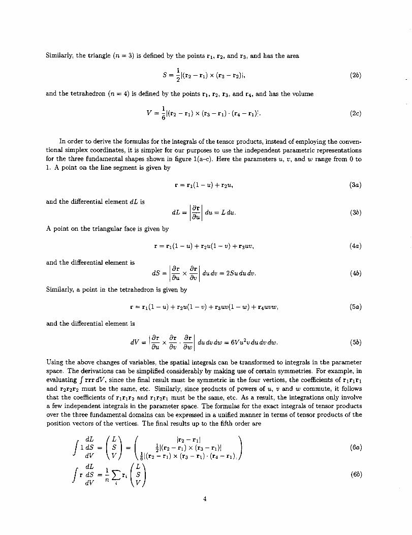
Quadrature approximation for integrals of an arbitrary function f over the fundamental domains are of

the form

[ /(r) dS = wj(rq) S , (ha)J dV V

where rq is a quadrature point and the coefficient wq is the corresponding weight. The approximation has

a degree of precision d if it is exact for all polynomials of degree equal to or less than d. Here we consider

only approximations which are symmetric with respect to the vertices. The quadrature points then fall into

symmetry groups, each of which is associated with a single weight. The quadrature approximation then

takes the form

1(;)f f(r) dS = Z f(rqg) (llb)dV q

where rqg is a quadrature point belonging to symmetry group g. The symmetry is most clearly evidentwhen viewed from the centroid of each fundamental shape. We therefore find it useful to introduce a

parameterization based on the centroid, rather than the conventional simplex coordinates, to classify the

quadrature points.

Let _ denote the position vector with respect to the centroid of the fundamental shape. Therefore

= r - r c, (12)

where

defines the centroid. It is easy to show that

1rC - n E r_ (13)

r_ = o. (14)i

From the above equation, it follows that in evaluating the integrals of tensor products of f, all summations

in which any index appears once also vanish. For the line segment, since _1 = -_2, we then obtain

/rdL=/_dL=/f_f_rdL=O.

The remaining eqs. (6) and (7) in terms of centroid based position vectors reduce to

f dSi dV =0

dL

/ _ dSdV

f .s_ dV

_ dS =

f _iii dV =

..... dSrrrrr dV =

(15a)

(15b)

-- n(n + 1) _. _i_i (15c)

2 (S) (15d)= n(n + 1)(n+ 2) Er_riri V

n(n + 1)(n + 2)(n + 3) Z. ii_i_¢

_(n + 1)(n + 2)(_ + a) [ _(_,ej_j +...) + 6_ _,e_e,_,l V (15/)j i

n(n + 1)(n + 2)(n + 3)(n + 4) E r_r_r_rir_ • (15g)

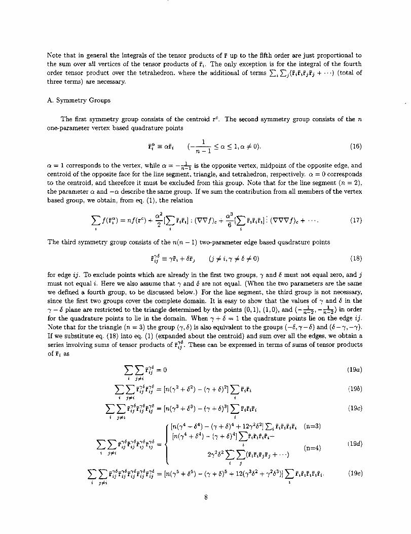
Notethat in general the integrals of the tensor products of f up to the fifth order are just proportional to

the sum over all vertices of the tensor products of _i. The only exception is for the integral of the fourth

order tensor product over the tetrahedron, where the additional of terms _":_i_'_j(rir_rjrj +'" ") (total of

three terms) are necessary.

A. Symmetry Groups

The first symmetry group consists of the centroid r c. The second symmetry group consists of the n

one-parameter vertex based quadrature points

1r-P-afi (---<a<l,a#0).n_l- - (16)

a = 1 corresponds to the vertex, while a = -_-1 is the opposite vertex, midpoint of the opposite edge, and

centroid of the opposite face for the line segment, triangle, and tetrahedron, respectively, a = 0 corresponds

to the centroid, and therefore it must be excluded from this group. Note that for the line segment (n = 2),

the parameter a and -a describe the same group. If we sum the contribution from all members of the vertex

based group, we obtain, from eq. (1), the relation

0c2 _3

_-_ f(T_) ----nf(r c) + T[_"_ _i_=] : (VVf)c + -_-[E _iTi_i] " (VVVf)c + -.-. (17)

The third symmetry group consists of the n(n - 1) two-parameter edge based quadrature points

,_ - 7h + 6_j (j # i, 7 # 6 # 0) (18)

for edge ij. To exclude points which are already in the first two groups, 7 and _ must not equal zero, and j

must not equal i. Here we also assume that 7 and 6 are not equal. (When the two parameters are the same

we defined a fourth group, to be discussed below.) For the line segment, the third group is not necessary,

since the first two groups cover the complete domain. It is easy to show that the values of 7 and 6 in the

7 - 6 plane are restricted to the triangle determined by the points (0, 1), (1,0), and ( 1 ! ) in ordern-2' n-2

for the quadrature points to lie in the domain. When 7 + 6 = 1 the quadrature points lie on the edge ij.

Note that for the triangle (n = 3) the group (7,/5) is also equivalent to the groups (-6, 7 - 6) and (6 - 7, -7).

If we substitute eq. (18) into eq. (1) (expanded about the centroid) and sum over all the edges, we obtain a

series involving sums of tensor products of t'Y*ij. These can be expressed in terms of sums of tensor products

of _i as

z_,XT"_=_j = 0 (19a)i j#i

-_ _'_='_z_., i.__ij = [n(72 + 62) - (7 + 6)2]_ _di (19b)i j#i i

z..., i3 ,_ '-i3 = [n(73 + 63) - (7 + 6)3] _ ririr, _19c)i j-#i i

{ [n(74 + _4) _ (7 + 6)4 + 127 _6_] _, hh_,_, (n=3)_/_ _-_ff'_=.'_6='_6 [n(74 + 64) -- (7 + ¢5)4] _-_ffiririri+

+ ...)j

_ij xij "ij "ij Lij = [n( "/5 + 65) -- ('T + 6) 5 + 12(7362 + 'T2_3)] _ ririririri. (19e)

i 3#i i

In deriving the above equations, we made use of the same simplifications that were employed to obtain

eqs. (7). The fourth symmetry group is a degenerate case of the third symmetry group when 3' = 6 _=/3,

and consists of the n(n - 1)/2 one-parameter edge based quadrature points

P_ --/3(Pi+ Pj) (j>i, 1 </3< 1n- 2 - - _'/3 # 0). (20)

/3 = ½ corresponds to the midpoint of the edge ij. This _oup is not necessary for the triangle (n = 3), sincethe vertex based group already includes this case. We therefore show results for the tetrahedron (n = 4) only.

For this case the parameter 13 and -/3 describe the same group. The relevant tensor product summations

over the edges can then be expressed as

i j>i

_V" P.P. = 2__Z _'_'i j>i i

i3 ij ij

i j>i

E E rijrijrijr'J = _'[E E (FiFifjrj + "" ") -4 E r,r,rir,]i j>i i j i

rijrijrijrijrij = O.

i j>i

(21a)

(215)

(21c)

(21d)

(21_)

The conventional simplex coordinate #i are defined by

where

r = E#ir_, (22a)i

E #i = 1. (225).

It is easy to establish the relations between our centroidal parameterization and the conventional simplex

coordinates for the four symmetry _oups as follows:

1For r c : /zi = - (for all i)

n

1 + (n - 1)ar_-: /zi

n

m = _ (j # i)n

1 + (n - 1)7 -_w6ij : ,ui =

/zj =

n

1 - 7 + (n- 1)6

n

1 -7-6

n

1 + (n - 2)_#i = #5 -

1- 2/3P,k--

n

n

(k # i, k # j)

(k#i,k#j)

(23)

(24a)

(24b)

(25a)

(255)

(25c)

(26a)

(26b)

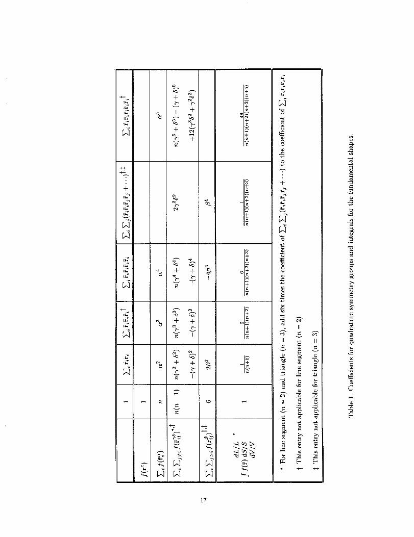
Theresultscontainedineqs.(15),(17),(19),and(21)canbesummarizedin table1. It showscoefficientsmultiplyingthevarioustensorproductsummationsforeachofthesymmetrygroups,aswellastheintegralof f([) over the fundamental domains. Note that for n = 2 or 3, the column _i _-'_q(ririrjrj +'") isnot applicable, but six times the coefficients in that column must be added to the coefficients in column

_-_i r_rir_f_. All s)nnmetric quadrature formulas of any degree of precision up to five can be derived from this

table. The number of independent terms (columns) required for a given degree of precision depends on the

fundamental shape. For the line element, the degree of precision d of the quadrature approximation equals

one plus two times the number of independent terms. For the other two shapes, an approximation of degree

of precision d has d independent terms, except for the tetrahedron, where we have d + 1 terms if d _> 4.

In a Gauss quadrature formula, the parameters defining a symmetry group are unspecified. Then the

number of unknowns associated with a group is one (the weight) plus the number of parameters defining the

group. The number of quadrature points belonging to a symmetry group is a function of the fundamental

shape. The efficiency of a particular symmetry group in forming a Gauss quadrature approximation is

measured by the number of quadrature points per unknown. These are tabulated for the four symmetry

groups and three fundamental shapes in table 2. For the line element, the two symmetry groups are equally

efficient, but for the other two shapes the efficiency is a function of the symmetry group, with the centroid

being the most efficient and the two-parameter edged based group being the least efficient. The latter group

is not required to derive the most efficient Gauss quadrature formulas when the degree of precision is no

greater than five. But that group is important in obtaining efficient Lobatto formulas, as will be shown

below. Using tables 1 and 2 we can derive Gauss quadrature formulas for the three fundamental shapes by

equating the total number of unknowns to the number of independent terms. There may be more than one

combination of symmetry groups satisfying this condition. The combination giving the most efficient formula

will be referred to as the Gauss quadrature formula. Since the parameters occur nonlinearly for d _> 2, there

may be more than one solution for a particular combination of symmetry groups. This will be found to be

true for one case even after discarding solutions that locate quadrature points outside the domains. For the

triangle and tetrahedron, the formulas may contain negative weight coefficients.

While the Gauss quadrature formulas are the most efficient for isolated fundamental shapes, they may

not be appropriate if positive weight coefficients are desired or if the shapes are part of a grid in which their

boundaries (vertices, edges, or faces) are shared by several neighbors. In these cases it may be more efficient to

employ limiting forms of the symmetry groups in which the points lie on the boundary elements. Quadrature

formulas using these special symmetry groups will be referred to as Lobatto. These new symmetry groups

-e face centroids _./, and one-parameter edge points -_ Theyconsist of the vertices -v edge midpoints rq,ri, rij.are defined as

and

-v - (2r)r i --r_ witha=l;

i_j - _ with a -- -½, vertex k opposite edge ij, for triangle; (28a)

- f_ with/3-- ½, for tetrahedron; (28b)

_{ -- ri-_ with a = -½, vertex i opposite face f, for tetrahedron; (29)

_j - _ (30)q with_/=e,_=l-e.

In order to determine the relative efficiency of these new symmetry groups, we need the relations among the

fundamental elements (vertices, edges, faces, and cells) which make up an arbitrary polygon or polyhedron.

For a polygonal face (or plane polygon in two dimensions), which can always be triangulated without

introducing interior vertices, we define

v = number of vertices. (31a)

10

and

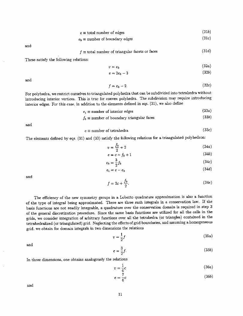
e -- total number of edges

eb = number of boundary edges

f -- total number of triangular facets or faces

These satisfy the following relations:

and

(31b)

(31c)

(31d)

v = eb (32a)

e = 2eb -- 3 (32b)

f = eb -- 2. (32C)

For polyhedra, we restrict ourselves to triangulated polyhedra that can be subdivided into tetrahedra without

introducing interior vertices. This is true for convex polyhedra. The subdivision may require introducing

interior edges. For this case, in addition to the elements defined in eqs. (31), we also define

ei - number of interior edges (33a)

fb =--number of boundary triangular faces (33b)

and

c - number of tetrahedra (33c)

The elements defined by eqs. (31) and (33) satisfy the following relations for a triangulated polyhedron:

and

fb (34a)

e = c+ h + 1 (34b)

eb= (34c)

ei = e - eb (34d)

f --- 2c + --.fb (34e)2

The efficiency of the new symmetry groups in a Lobatto quadrature approximation is also a function

of the type of integral being approximated. There are three such inte_als in a conservation law. If the

basis functions are not readily integrable, a quadrature over the conservation domain is required in step 3

of the general discretization procedure. Since the same basis functions are utilized for all the cells in the

grids, we consider integration of arbitrary functions over all the tetrahedra (or triangles) contained in the

tetrahedralized (or triangulated) grid. Neglecting the effects of _id boundaries, and assuming a homogeneous

grid, we obtain for domain integrals in two dimensions the relations

1 (35a)v = _f

and3

In three dimensions, one obtains analogously the relations

1

7

e_ c

and

(35b)

(36a)

(36b)

11

f = 2c. (36e)

The second type of integral is a source integral. This involves integrating an arbitrary non-linear function

over a polyhedral (or polygonal) cell. The relations among the geometric elements are given by eqs. (32)

and (34). The third type of integral is a boundary integral. For each function evaluation at a boundary

point, several additional projections onto the boundary normals or tangents may be required. We assume

that the computational cost of these projections can be neglected compared to the computational cost of

the function evaluation. For two-dimensional problems the boundaries are line segments, and the Gauss

formula is to be preferred. For three-dimensional problems, the required relations for the boundary of a

triangulated polyhedra are given by eqs. (34b) and (34c). The data for each boundary symmetry group

obtained from eqs. (32), (34), (35), and (36) is tabulated for the three types of Lobatto integrals in table 3.

For completeness, we have also repeated the information for the group r c and _. All Lobatto formulas can

be obtained using tables 1 and 3, where entries in table 1 are replaced by their limiting values as indicated

in eqs. (27) to (30). For a given degree of precision, there are now many more combinations of symmetry

groups to evaluate as possible candidates. Again, we may find several or no solutions, and will discard those

with quadrature points outside the domains.

The last column in table 3 deserves further comments. For a given polyhedron, increasing the number

of interior edges increases the total number of tetrahedral cells, faces, and edges, but the total number of

vertices remains the same. Therefore, the net result is to increase the total total number of quadrature

points for every symmetry group except the group r_.-v Whenever possible, one should triangulate polygonal

faces and subdivide the triangulated polyhedron in such a way as to minimize the number of interior edges,

which also minimize the number of tetrahedral cells. We illustrate this point with some simple examples. A

tetragonal pyramid with a planar base, which has five vertices, can only be subdivided into two tetrahedra

with no interior edge. But a trigonal bipyramid, which also has five vertices, can be subdivided into two

tetrahedra with no interior edge, or three tetrahedra with one interior edge. The former subdivision is to be

preferred, since it results in fewer total number of quadrature points. There are two important shapes with

six vertices. An octahedron can only be subdivided into four tetrahedra with one interior edge. A trigonal

prism can be subdivided into three or four tetrahedra, depending on the triangulation of the quadrilateral

faces. It is easy to prove that an arbitrary trigonal prismatic grid can always be triangulated so as to result

in three tetrahedra per prism with no interior edge. Another example is a structured grid consisting of

hexahedra with quadrilateral faces. As shown by Rizzi (ref. 7), there exists a triangulation of the faces

which permits subdivision into five tetrahedra with no interior edge. One of the five is twice the size of the

other four. Kordulla and Vinokur (ref. 8) recommended a subdivision into six tetrahedra, by introducing

a main diagonal as a common interior edge. Although the latter produces a more uniform subdivision, the

former is preferred. In summary, polyhedra consisting of less than four tetrahedra will not require an interior

edge, while those with four or more may require one.

B. Quadrature Formulas

With the aid of tables 1-3, we can derive virtually all symmetric quadrature formulas of any degree

of precision up to five. By choosing different combinations of symmetry groups one might end up with

more unknowns than the number of equations required to be solved. The resulting system of equations thus

becomes under-determined, and the solutions can then be expressed in terms of free parameters. We can

show that many published formulas are just solutions with particular choices of the free parameters. We have

tabulated some Gauss and Lobatto formulas that are useful for approximating the different types of integrals

for arbitrary polyhedral and polygonal grids. Only those formulas for which the quadrature points lie within

the domains are given. The formulas for the line element are classical, and therefore are not presented. The

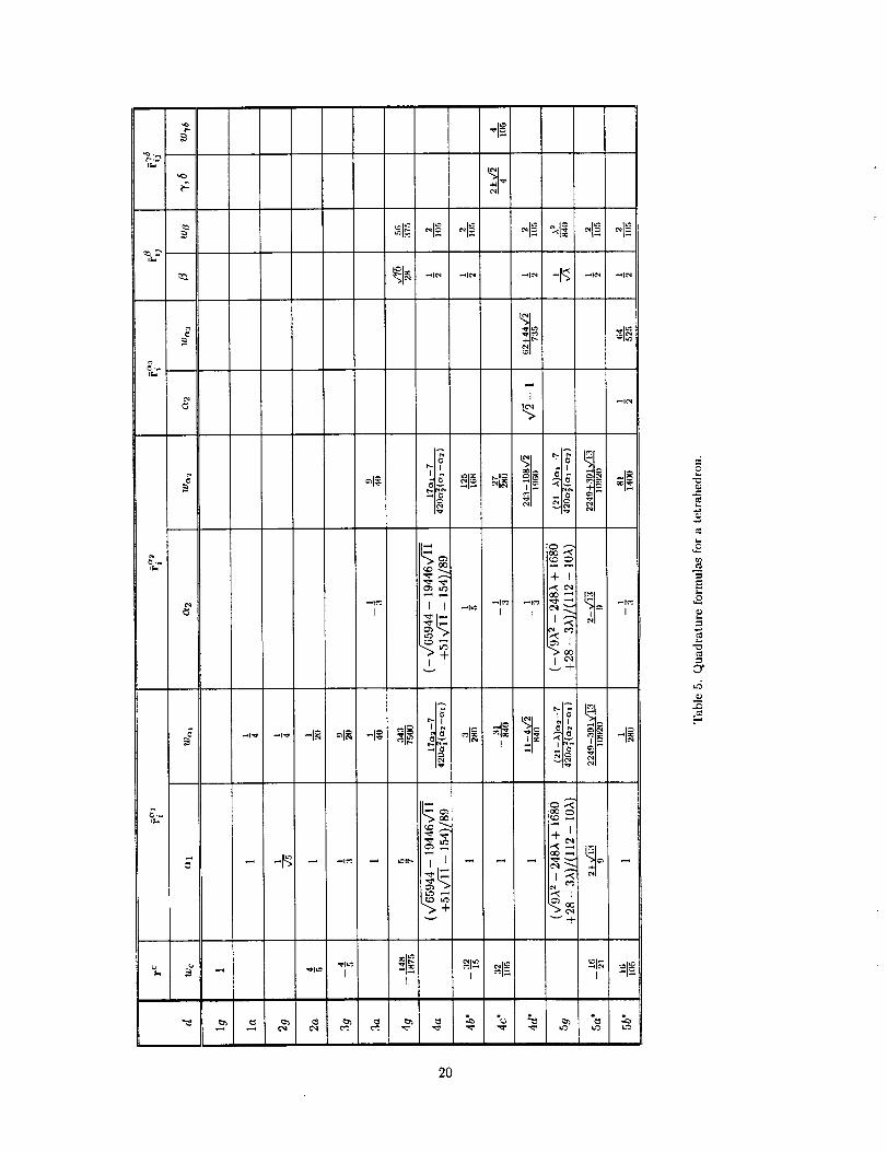
coefficients for triangles and tetrahedra are given in tables 4 and 5, respectively. Although they can all be

12

expressedinclosedform,dueto spacelimitations,oneoftherelationsisgivenin thetextbelow.Theletterg refers to Gauss formulas, while the other letters indicate Lobatto formulas. Those formulas not found in

references cited in this paper are starred. Note that negative weights are present in formulas 3g and 4c for

triangles, and 3g, 4g, 4b, 4c, and 5a for tetrahedra.

We now give brief derivations of some the formulas, concentrating on those combinations of symmetry

groups resulting in the solution of quadratic or cubic algebraic equations. As can be seen from tables 2 and

3, the edge-based symmetry groups f_/and f_'_3and their limiting forms are less efficient than the centroid r c

and vertex-based symmetry group fa and its limiting form. None of the edge-based groups or their limitingZ '

forms are required until we reach d _ 4. We note from table 1 that if the centroid r e is present, the weight

wc appears only in the first column. The system is thus simplified, having been reduced by one equation

and one unknown. A unique solution is then readily obtained for all the cases we tabulated except for d -- 5,

where two formulas require the solution of a quadratic equation.

It follows from table 1 that for d < 3 the triangle and tetrahedron may be treated in a unified manner.

From table 2 we see that an n-point Gauss formula for d = 2 is given by the symmetry group f_. From the

first two columns of table 1 we obtain immediately

1 1 (37)d=2: w_=-n and a=±vr_+ 1

For the tetrahedron (n = 4) the negative root must be discarded, since a is outside the permitted range (see

eq. (16)). For the triangle (n = 3) both roots are valid, but the negative root (a = _1)2 places the points on

the mid-edge of the triangle. According to our definition it is still a Gauss formula, with a Lobatto flavor,

since it actually employs the mid-edge symmetry group f ej. It therefore has superior properties, and is to

be preferred to the positive root. From table 3 we see that it is also superior to the true Lobatto formula

based on r e and f_ for the source and boundary integrals, but equally as efficient for the domain integral.

Using tables 1 and 2, we readily derive the solution for the n + 1 point Gauss formula for d -- 3, based on

r e and f_$,as

n2 (n + 2)2 2 (3s)d= 3 : wc = n(n + l)' wc_ = 4n(n + l)' _=n'_'

-v and f_Note that the centroid has a negative weight for both shapes. The Lobatto formula based on r i

involves the solution of a quadratic equation. The final expressions are

17=v/_+9 2n2+6n+3± 4_9 l±v/_+9 (39)d= 3 : wv = 2n(n + l)(n + 2)' wa= 2n(n + l)(n + 2) , a= 2(n+2)

The two roots for c_ are within the permitted range for both shapes, but only the lower sign gives all positive

weights. For the tetrahedron, there is an additional reason for choosing the lower sign, since we have a = -½,

-v and f./, and all the points lie on the boundary. On the otherso that the formula is actually based on r i

hand, one can show from table 3 that for the triangle the Lobatto formula based on r e, f_, and f ej is more

efficient than eq. (39) for the domain and boundary integrals.

When d >_ 4, it follows from column 5 in table 1 that the formula for a tetrahedron requires the symmetry

groups f_ or f_ij, or their limiting forms. The use of the two-parameter edge-based group is in general lessefficient than using the combination of one-parameter edge-based and vertex-based groups. When employing

f_, one can derive from table I the relation

1 (4o)wzZ4 = s4---o

13

Oneimmediatelyobtainswe = _ for Lobatto formulas involving the edge midpoint symmetry group _i_.For these cases, the solutions for tetrahedra have the same structure as those for the corresponding triangles.

All the quadrature formulas except two for d > 4 that we have tabulated include two vertex-based

symmetry group _ and _2, or their limiting forms. Here we present a general method for obtaining

solutions, although many Lobatto formulas can be determined by simpler procedures. The equations to be

solved are some or all of the set

Wal _ Wa2 = ao

_/2a10_12 "_- wa:20_22 _ a2

walo_l 3 -_- 2/2a2_23 -- a3

walo_l 4 -_- Wa20_24 _ a4

walo_l 5 --_ wa2(_25 _ a 5.

(41a)

(41b)

(41c)

(41d)

(41e)

The parameters ai could include unknowns from other symmetry groups. From eqs. (41b) and (41c) we

obtain for wa 1 and wa 2 the expressions

- a2al - a3 (42)= a2a2 a3), w_=_2s(___s).Wc_l _12(O_ 2 __ Oil

Substituting the above equations into eqs. (41a), (41d), and (41e) we obtain

a_(_, + _s) - as [(_ + _s) s - _2)] = a0(_s) s

a3(al + a2) -- asala2 = a4

_3 [(_ + _s)2 - a1_2] - a_las(_l + _s) = as.

(43a)

(435)

(43c)

For d = 4, we can eliminate (al + c_2) by substituting eq. (43b) into eq. (43a), and obtain for ala2 the

quadratic equation

(a23 -- aoa32)(ala2) 2 + 2a2(asa4 -- a32)ala2 +a4(asa4 - a32)--0. (44)

If there are no additional unknowns from other symmetry groups, and for the values of a0 to a4 in our

tabulated cases, eq. (44) has two real solutions. For each of them, eq. (43a) then yields a quadratic equation

whose solutions are al and c_2. In our cases the constants are such that one of the solutions of eq. (44)

results in locating one a outside the permitted range. For d = 5, it follows from eqs. (43b) and (43c) that

al and as are two solutions of the quadratic equation

(asa4 - a3S)a s + (a3a4 - a2as)c_ + (a3as - a4 s) = O. (45)

As an example, we present the Gaussian solution for the tetrahedron for the degree of precision five. The

most efficient quadrature points for this case involve two vertex-based _ and one edge-based [_ symmetry

groups. (The Gauss formula _ven in ref. 5 is less efficient than the present one.) We must now include

eq. (40) in our equation set (41). In terms of1

A - (46)_2,

1 As 1 Aa0 = - ---- a2=

4 560' 20 420'1 1 1

a3 =_-_, a4 =_, and a5 = 14--0"

the parameters a_ become

(47)

14

Substituting(al + a2) and ala2 from eq. (45) into eq. (43a), one obtains a cubic equation for A

9A 3 - 284A 2 + 2800A - 8512 = 0. (48)

The above equation has three real roots. The values of al and a2 from one root are complex, while those

from another root place one set of points outside the tetrahedron. The remaining root is given

24964 -']- 71 .

3(49)

This value must be used in evaluating formula 5g in table 5. Note that this formula was derived in reference 2

by an entirely different procedure, but only numerical values of the parameters were given. We have provided

explicit exact relations for the parameters.

For a given degree of precision d, the optimum quadrature formulas to use (in terms of the minimum

number of quadrature points) depend on the type of integral being approximated, and whether negative

weights are allowed. For each value of d, using tables 1-3, we have examined all possible candidate combi-

nations of symmetry groups to determine the optimum one. The results are summarized in table 6. In the

w column, "pos" means that positive weights are necessary, while "neg" means that negative weights are

allowed. For triangles, the formulas for the domain integrals were previously given in reference 4. One final

note concerns the domain integral for a tetrahedron. For a non-uniform _id obtained by subdividing the

hexahedron of a structured grid into five tetrahedra, the entries in table 3 for the groups r_-V,r_j-¢, and r_j-_

would be ½ 6 _,, _, and respectively. This does not affect the choice of optimum formulas in table 6.

IV. Concluding Remarks

We have presented formulas for exact inte_als of polynomials and quadrature approximations up to

degree five for the line segment, triangle, and tetrahedron. These three shapes are the building blocks for

integrations over arbitrary polyhedral or polygonal grids. A table of coefficients for quadrature symmetry

groups and integrals for all three shapes is given, enabling one to construct symmetric quadrature formulas

in a rational manner. The new procedure for obtaining the solutions in higher dimensions is no more complex

than the one we are familiar with for one dimension. We have tabulated many useful Gauss and Lobatto

formulas for both the triangle and tetrahedron, including a number that have not appeared in references

available to us. All the formulas derived in this paper provide necessary tools in the spatial discretization of

finite-volume equations over arbitrary polyhedral or polygonal _ids to an accuracy of up to the fifth order.

Higher-order formulas can be readily obtained using our procedure. Some of the quadrature formulas will

now require the introduction of the two-parameter edge based symmetry group defined by eq. (18). As a

result, the coefficients will not always be expressible in closed form, but may require the numerical solution

of non-linear algebraic equations.

15

References

1. Stroud, A. H.: Approximate Calculation of Multiple Integrals. Prentice-Hall, New Jersey, 1971.

2. Grundmann, A.; and M611er, H. M.: Invariant Integration Formulas for the n-Simplex by Combinatorial

Methods. SIAM J. Numer. Anal., vol. 15, no. 2, 1978, p. 282.

3. Cowper, G. R.: Gaussian Quadrature Formulas for Triangle. Int. J. Num. Meth. Eng., vol. 7, 1973,

p. 405.

4. Lyness, J. N.; and Jespersen, D.: Moderate De_ee Symmetric Quadrature Rules for the Triangle.

J. Inst. Maths. Applics, vol. 15, 1975, p. 19.

5. Yu, J.: Symmetric Gaussian Quadrature Formulae for Tetrahedronal Regions. Comput. Meth. Appl.

Mech. Eng., vol. 43, 1984, p. 349.

6. Keast, P.: Moderate-Degree Tetrahedral Quadrature Formulas. Comput. Meth. Appl. Mech. Eng.,

vol. 55, 1986, p. 339.

7. Rizzi, A.: Damped Euler Equation Method to Compute 2_ansonic Flow Around Wing-Body Configu-

rations. AIAA J., vol. 20, 1982, p. 1321.

8. Kordulla, W.; and Vinokur, M.: Efficient Computation of Volume in Flow Predictions. AIAA J., vol. 21,

1983, p. 917.

(a) line segment (b) triangle (c) tetrahedron

r3 r 4

U W

v r3

2

Figure 1. Parametric representations for the three fundamental shapes.

16

tkq

r_

J_

t_J

IL.

iL.

IL.

%

%

%

÷ _

L_ v_

%

÷ ÷

÷ ÷

÷ ._-

vt_

+

+

+

÷

v

÷

o

÷

t L.

v

_L.4

_EC_

._x

il

_o

_t

v

_o

It

v

_ Lt

.__ ._

_ rJ_

a_

c_

cs_

ot_D

©

17

Z

0 1.0

°_

bO

°_

Z

0

Z

Z

u_e_

o

"0

Z

c,i

_o ÷ ÷ ÷ ÷

0

"el

o + + +

_ .-_0

Z _

_6

o

D.

o0_

0

0

Z

N

¢

18

11,4

[.,.

4-

..I._

I

e_

II,._

oc

Le)

_7

I

7

-,_ -,_ -i-_ _.i.. -I_ o_I_ -i_ _

o"

e,

#

I

+

+

I

I

19

_I__I_ _I_

_I_-'_-'_

LS.

I

=-I_

I I --t_ I I _ _ = I

_I___ _ _,_ -I_

0

.=

r_

+_

_'_ _- _I_ _I__I_"_" I I I

I

2O

o

bO

°_

o

OO_

..=

O

O

O

O

_6 _6© O

-+-- 4-.-

fl A _ VIAI

¢q O,l ¢'0 eO

v AI V AI II A

O _ O O ¢_

I_ A

O o O o

¢'O

_o

O

°_

.e--

°_

O

©

21

Form Approved

REPORT DOCUMENTATION PAGE oMBNo OZO4-OlOS

PublicreportingburOen for this collectionof informationis estimatedto average 1hour per response,includingthe time for reviewing instructions, searchingexisting data sources,gatheringand maintaining the data needed, and completingand reviewingthe collectionof information. Send commentsregardingthis burdenestimate or any other aspect of thiscollectionof information, including suggestionsfor reducingthis burden,to WashingtonHeadquartersServices, Directorate for informationOperationsand Reports, 1215 JeffersonDavis Highway,Suile 1204, Arlington.VA 22202-4302. anclto the Office of Managementand Budget, PaperworkReductionProject(0704o0188), Washington, DC 20503

1, AGENCY USE ONLY (Leave blank) 12" REPORT DATE 3, REPORT TYPE AND DATES COVERED

I June 1997 Technical Memorandum

,4. TITLE AND SUBTITLE 5. FUNDING NUMBERS

Exact Integrations of Polynomials and Symmetric Quadrature Formulas

over Arbitrary Polyhedral Grids

16. AUTHOR(S)

Yen Liu and Marcel Vinokur

'7. PERFORMINGORGANIZATIONNAME(S)ANDADDRESS(ES)

Ames Research Center

Moffett Field, CA 94035-1000

9. SPONSORING/MONITORING AGENCY NAME(S) AND ADDRESS(ES)

National Aeronautics and Space Administration

Washington, DC 20546-0001

522-31-12

8. PERFORMING ORGANIZATIONREPORT NUMBER

A-976805

10. SPONSORING/MONITORINGAGENCY REPORT NUMBER

NASATM-112202

11. SUPPLEMENTARY NOTES

Point of Contact: Marcel Vinokur, Ames Research Center, MS T27B-1, Moffett Field, CA 94035-t000

(415) 604-4736

12a. DISTRIBUTION/AVAILABILITY STATEMENT

Unclassified -- Unlimited

Subject Category 64

12b. DISTRIBUTION CODE

13. ABSTRACT (Maximum 200 words)

This paper is concerned with two important elements in the high-order accurate spatial discretization of finitevolume equations over arbitrary grids. One element is the integration of basis functions over arbitrary domains, whichis used in expressing various spatial integrals in terms of discrete unknowns. The other consists of quadrature approxi-mations to those integrals. Only polynomial basis functions applied to polyhedral and polygonal grids are treated here.Non-triangular polygonal faces are subdivided into a union of planar triangular facets, and the resulting triangulatedpolyhedron is subdivided into a union of tetrahedra. The straight line segment, triangle, and tetrahedron are thus thefundamental shapes that are the building blocks for all integrations and quadrature approximations. Integrals ofproducts up to the fifth order are derived in a unified manner for the three fundamental shapes in terms of the positionvectors of vertices. Results are given both in terms of tensor products and products of Cartesian coordinates. The exactpolynomial integrals are used to obtain symmetric quadrature approximations of any degree of precision up to five forarbitrary integrals over the three fundamental domains. Using a coordinate-free formulation, simple and rationalprocedures are developed to derive virtually all quadrature formulas, including some previously unpublished. Foursymmetry groups of quadrature points are introduced to derive Gauss formulas, while their limiting forms are used toderive Lobatto formulas. Representative Gauss and Lobatto formulas are tabulated. The relative efficiency of theirapplication to polyhedral and polygonal grids is detailed. The extension to higher degrees of precision is discussed.

14. SUBJECT TERMS

Quadrature formulas, Polyhedral grids, Finite volume

17. SECURITY CLASSIFICATIONOF REPORT

Unclassified

18. SECURITY CLASSIFICATIONOF THIS PAGE

Unclassified

19. SECURITY CLASSIFICATIONOF ABSTRACT

15. NUMBER OF PAGES

2416. PRICE CODE

A03

20. LIMITATION OF ABSTRACT

NSN 7540-01-280-5500 Standard Form 298 (Rev. 2-89)Prescribed by ANSI Std. Z39-1e

298-102