Exact Inference on Graphical Models Samson Cheung.

Exact Inference on Graphical Models

Samson Cheung

Outline

What is inference? Overview Preliminaries Three general algorithms for inference

Elimination Algorithm Belief Propagation Junction Tree

What is inference?

Given a fully specified joint distribution (database), inference is to query information about some random variables, given knowledge about other random variables.

Given a fully specified joint distribution (database), inference is to query information about some random variables, given knowledge about other random variables.

Evidence: xE

Query about XF?

Information about XF

Conditional/Marginal Prob.

Ex. Visual Tracking – you want to compute the conditional to quantify the uncertainty in your tracking

Evidence: xE

Conditional of XF?

Maximum A Posterior Estimate

Evidence: xE

Most likely valueof XF?

Error Control – Care about the decoded symbol. Difficult to compute the error probability in practice due to high bandwidth.

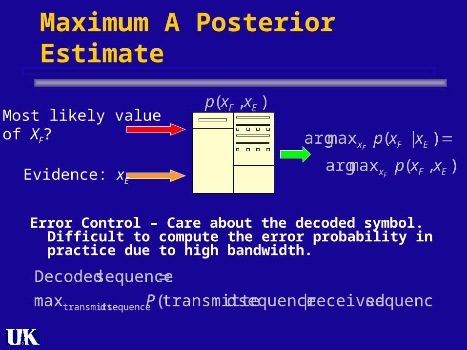
Inferencing is not easy

Computing marginals or MAP requires global communication!

Marginal:P(p,q)=G\{p,q} p(G)

Potential:(p,q) = exp(-|p-q|)

Evidence

Outline



Inference Algorithms

General Inference Algorithms

EXACT APPROXIMATE

General Graph

JUNCTIONTREE

ELIMINATIONALGORITHM

Polytrees

BELIEF PROPAGATION

1. Iterative Conditional Modes2. EM 3. Mean field4. Variational techniques5. Structural Variational

techniques6. Monte-Carlo 7. Expectation Propagation8. Loopy belief propagation

NP -hard

>1000 nodes:Image ProcessingVisionPhysics

10-100 nodes:Expert systemsDiagnosticsSimulation

Outline

What is inferencing? Overview Preliminaries Three general algorithms for inferencing

Elimination Algorithm Junction Tree Probability Propagation

Introducing evidence Inferencing : summing or maxing “part” of the

joint distribution

In order not to be sidetrack by the evidence node, we roll them into the joint by considering

Hence we will be summing or maxing the entire joint distribution

Calculating Marginal

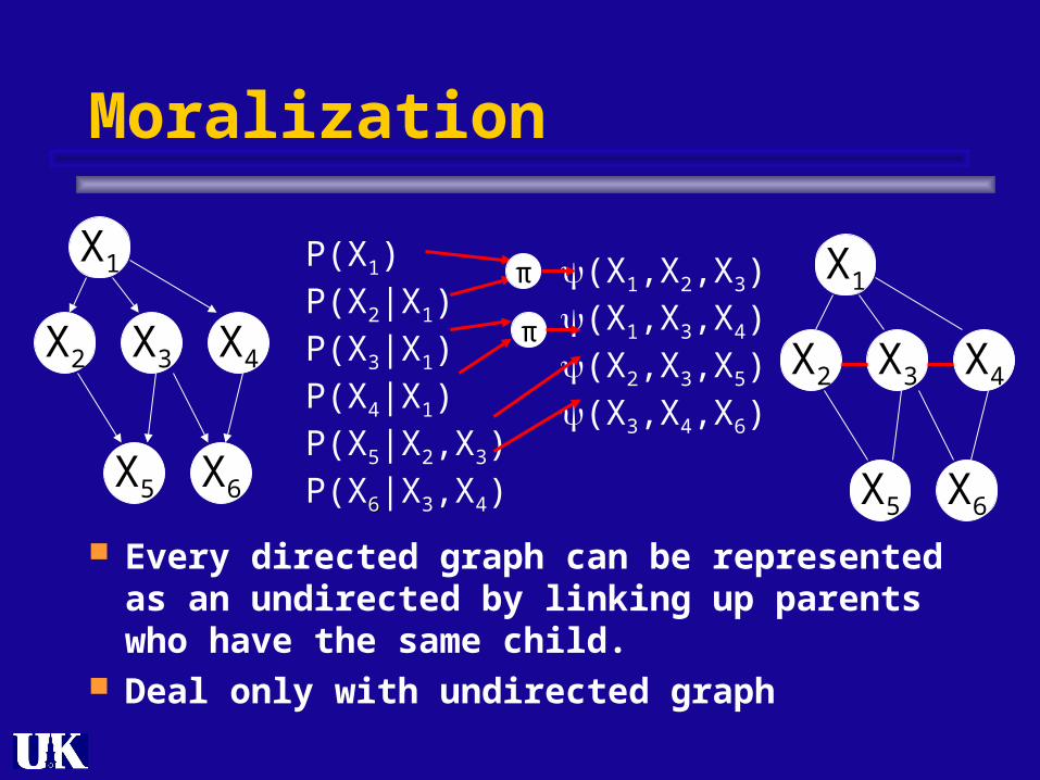
Moralization

Every directed graph can be represented as an undirected by linking up parents who have the same child.

Deal only with undirected graph

X2 X3

X1

X4

X5 X6

P(X1)P(X2|X1)P(X3|X1)P(X4|X1)P(X5|X2,X3)P(X66|X3,X4)

X2 X3

X1

X4

X5 X6

(X1,X2,X3)(X1,X3,X4)(X2,X3,X5) (X3,X4,X6)

π

π

Adding edges is “okay”

The pdf of an undirected graph can ALWAYS be expressed by the same graph with extra edges added.

A graph with more edge Lose important conditional independence information

(okay for inferencing, not good for parameter est.) Use more storage (why?)

X2 X3

X1

X4

X5 X6

(X1,X2,X3)(X1,X3,X4)(X2,X3,X5) (X3,X4,X6)

X2 X3

X1

X4

X5 X6

(X1,X2,X3,X4)(X2,X3,X5) (X3,X4,X6)

π

Undirected graph and Clique graph

Clique graph Each node is a clique from the parametrization An edge between two nodes (cliques) if the two

nodes (cliques) share common variables

X2 X3

X1

X4

X5 X6

C1(X1,X2,X3)

C2(X1,X3,X4)

C3(X2,X3,X5) C4(X3,X4,X6)

C5(X7,X8,X9)

C6(X1,X7)

X7 X8

X9

C1

C3

C2

C6

C4

C5

Separator:C1 C3={X2,X3}

Outline



Computing Marginal

Need to marginalize x2,x3,x4,x5

We need to sum N5 terms (N is the number of symbols for each r.v.)

Can we do better?

X1

X2

X3

X4

X5

Elimination (Marginalization) Order

Try to marginalize in this order: x5, x4, x3, x2

Complexity: O(KN3), Storage: O(N2) K=# r.v.s

C: O(N3)S: O(N2)C: O(N2)S: O(N)C: O(N3)S: O(N2)C: O(N2)S: O(N)

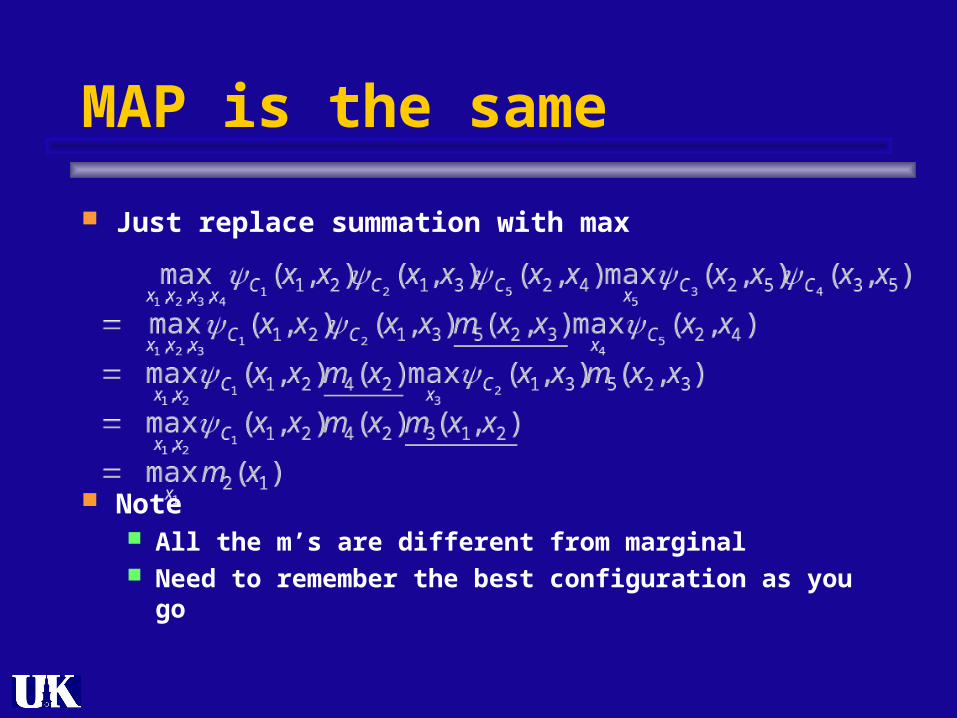
MAP is the same

Just replace summation with max

Note All the m’s are different from marginal Need to remember the best configuration as you go

Graphical Interpretation

X1

X2

X3

X4

X5

List of active potential functions:

C1(X1,X2)C2(X1,X3)C3(X2,X5)C4(X3,X5)C5(X2,X4)

C1(X1,X2)C2(X1,X3)C3(X2,X5)C4(X3,X5)C5(X2,X4)

C1(X1,X2)C2(X1,X3)C5(X2,X4)m5(X2,X3)

Kill X5

C1(X1,X2)C2(X1,X3)C5(X2,X4)m5(X2,X3)

C1(X1,X2)C2(X1,X3)m4(X2)m5(X2,X3)

Kill X4

C1(X1,X2)C2(X1,X3)m4(X2)m5(X2,X3)

C1(X1,X2)m4(X2)m3(X1,X2)

Kill X3

C1(X1,X2)m4(X2)m3(X1,X2)

m2(X1)

Kill X2

First real link to graph theory

Reconstituted Graph = the graph that contain all the extra edges after the elimination

Depends on the elimination order!

X3

X1

X2X4

X5

The complexity of graph elimination is O(NW), where W is

the size of the largest clique in the reconstituted graph The complexity of graph elimination is O(NW), where W is

the size of the largest clique in the reconstituted graph Proof : Exercise

Finding the optimal order

To minimize the clique size turns out to be NP-hard1

Greedy algorithm2:1. Find the node v in G that connects to the

least number of neighbors

2. Eliminate v and connect all its neighbors

3. Go back to 1 until G becomes a clique Current best techniques use other simulated

annealing3 or approximated algorithm4

1 S. Arnborg, D.G. Corneil, A. Proskurowski, Complexity of finding embeddings in a k-tree, SIAM J.Algebraic and Discrete Methods 8 (1987) 277–284.2 D. Rose, Triangulated graphs and the elimination process, J. Math. Anal. Appl. 32 (1974) 597–609.3U. Kjærulff, Triangulation of graph-algorithms giving small total state space, Technical Report R 90-09, Department of Mathematics and Computer Science, Aalborg University, Denmark, 1990.4A. Becker, D. Geiger, “A sufficiently fast algorithm for finding close to optimal clique trees,” Arificial Intelligence 125 (2001) 3-17

This is serious

One of the most commonly used graphical model in vision is Markov Random Field

Try to find a elimination order of this model.

Pixel: I(x,y)

(p,q) = exp(-|p-q|)

Largest clique: 4Grow linearly with dimension (?)

Outline



What about other marginals?

We have just computed P(X1).

What if I need to compute P(X1) or P(X5) ?

Definitely, some part of the calculation can be reused! Ex. m5(X2,X3) is the same for both!

X1

X2

X3

X4

X5

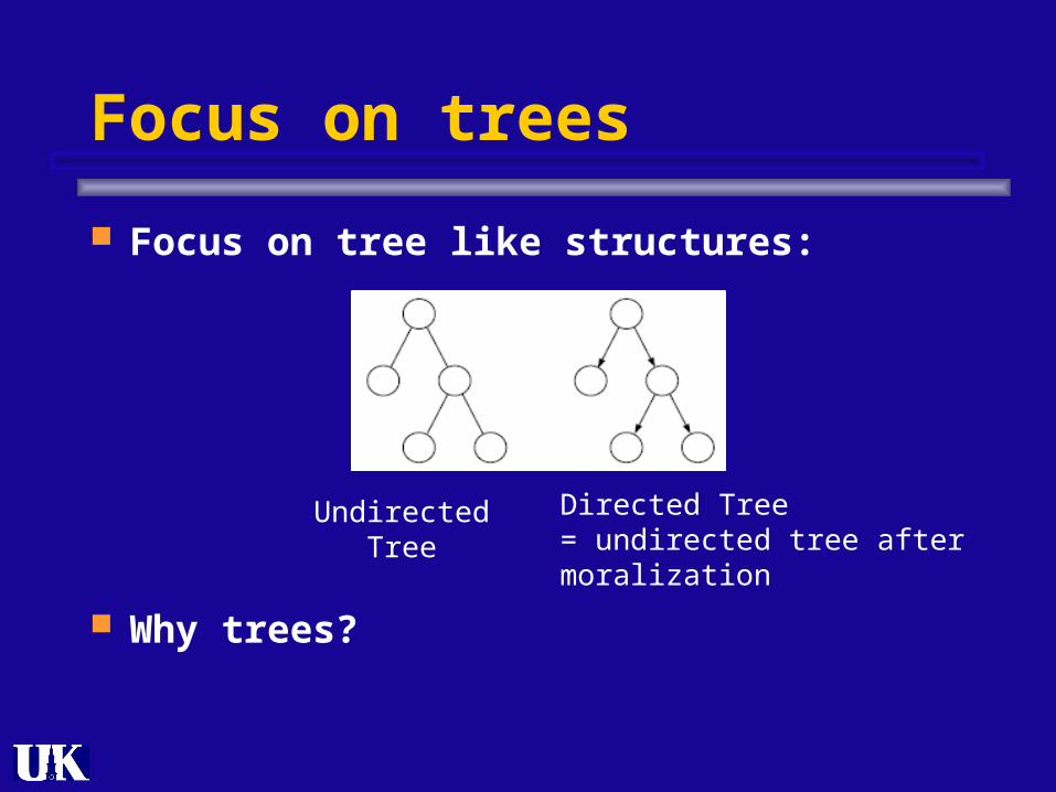
Focus on trees

Focus on tree like structures:

Why trees?

UndirectedTree

Directed Tree= undirected tree after moralization

Why trees?

No moralization is necessary

There is a natural elimination ordering with query node as root Depth first search : all children before parent

All sub-trees with no evidence nodes can be ignored (Why? Exercise for the undirected graph)

Elimination on trees

When we eliminate node j, the new potential function must be

A function of xi

Any other nodes? nothing in the sub-tree below j

(already eliminated) nothing from other sub-trees, since

the graph is a tree only i, from ij which relates i and j

Think of the new potential functions as a message mji(xi) from node j to node i

Think of the new potential functions as a message mji(xi) from node j to node i

mji(xi)

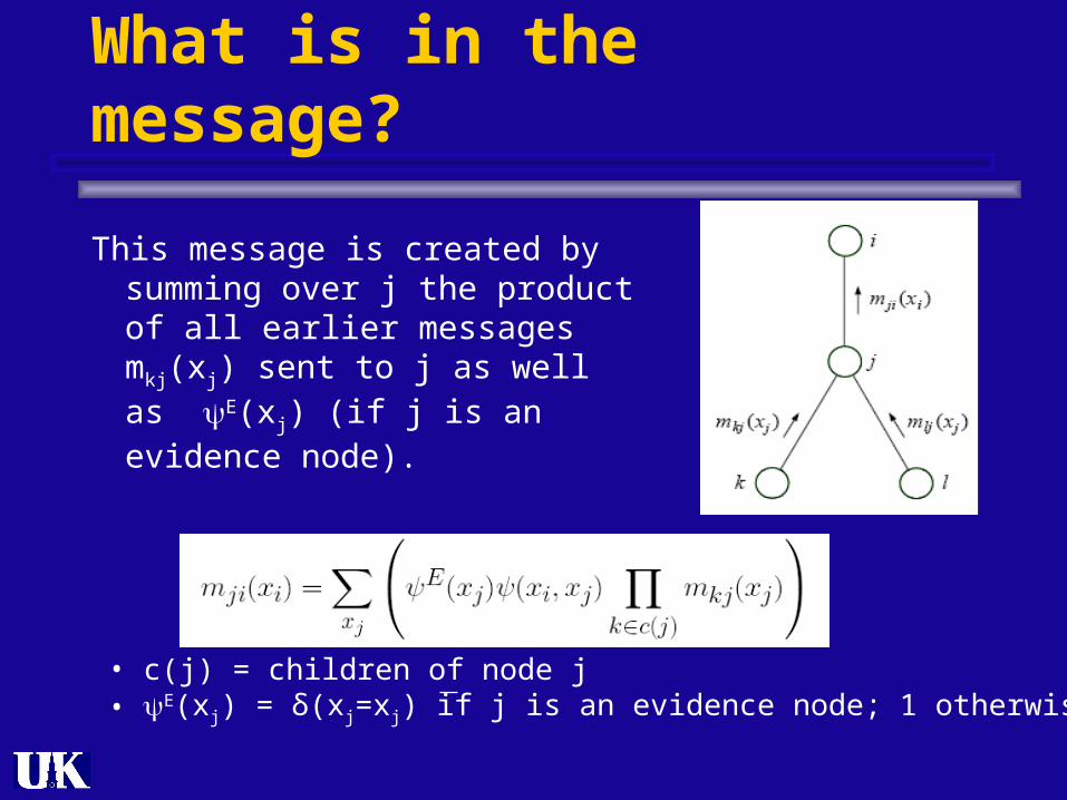
What is in the message?

This message is created by summing over j the product of all earlier messages mkj(xj) sent to j as well as E(xj) (if j is an evidence node).

• c(j) = children of node j• E(xj) = δ(xj=xj) if j is an evidence node; 1 otherwise

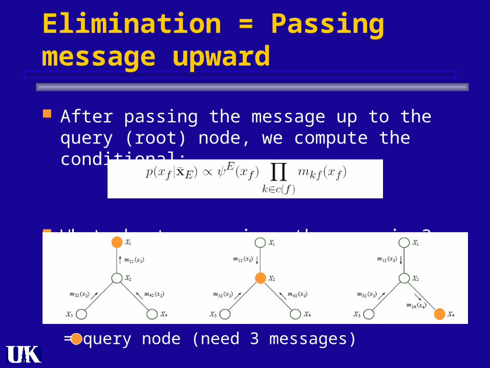
Elimination = Passing message upward

After passing the message up to the query (root) node, we compute the conditional:

What about answering other queries?

= query node (need 3 messages)

Messages are reused!

We can compute all possible messages in only double the amount of work it takes to do one query.

Then we take the product of relevant messages to get marginals.

Even though the naive approach (rerun Elimination) needs to compute N(N-1) messages to find marginals for all N query nodes, there are only 2(N-1) possible messages.

Even though the naive approach (rerun Elimination) needs to compute N(N-1) messages to find marginals for all N query nodes, there are only 2(N-1) possible messages.

Computing all possible messages

Idea: respect the following Message-Passing-Protocol:

A node can send a message to a neighbour only when it has received messages from all its other neighbours.

Protocol is realizable: designate one node (arbitrarily) as the root.

Collect messages inward to root then distribute back out to leaves.

Belief Propagation

i

j

k lmkj mlj

mji

mij

mjk mjl

Belief Propagation (sum-product)

1. Choose a root node (arbitrarily or as first query node).

2. If j is an evidence node, E(xj) = (xj=xj), else E(xj) = 1

3. Pass messages from leaves up to root and then back down using:

4. Given messages, compute marginals using:

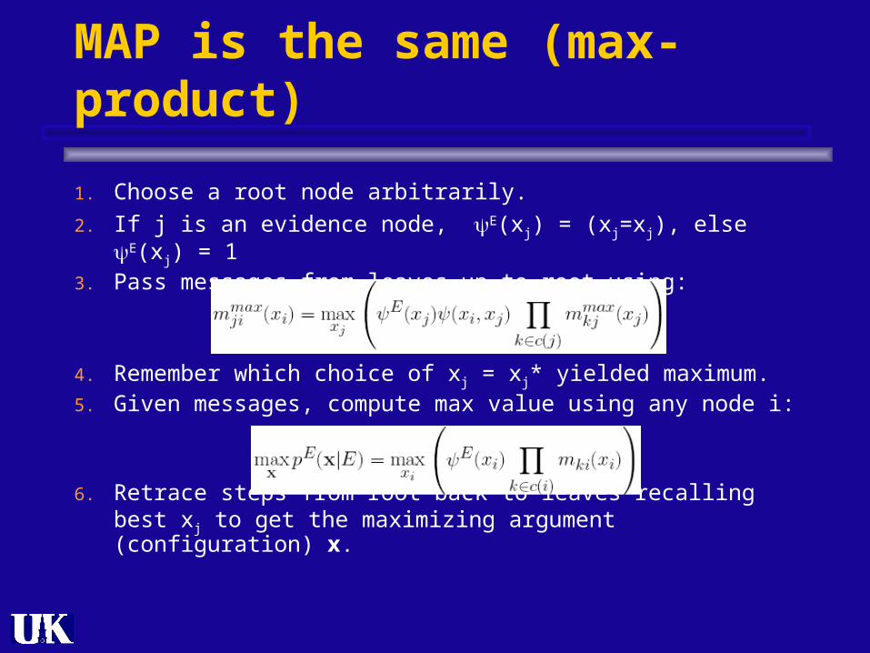
MAP is the same (max-product)

1. Choose a root node arbitrarily.

2. If j is an evidence node, E(xj) = (xj=xj), else E(xj) = 13. Pass messages from leaves up to root using:

4. Remember which choice of xj = xj* yielded maximum.5. Given messages, compute max value using any node i:

6. Retrace steps from root back to leaves recalling best x j to get the maximizing argument (configuration) x.

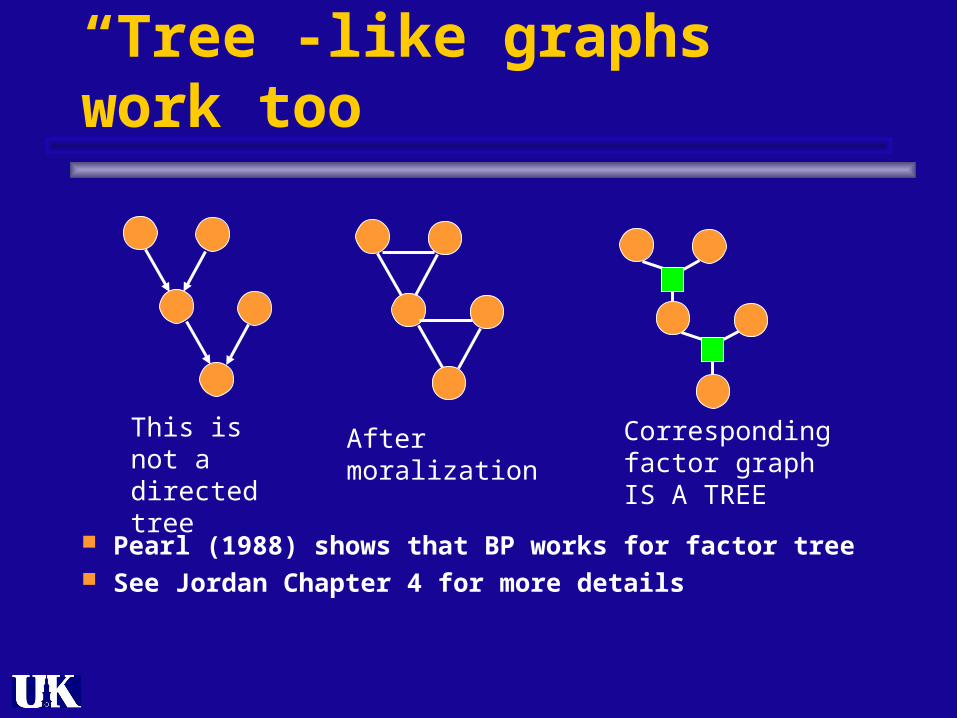
“Tree”-like graphs work too

Pearl (1988) shows that BP works for factor tree See Jordan Chapter 4 for more details

This is not a directed tree

After moralization Corresponding factor graph IS A TREE

Outline



What about arbitrary graphs?

BP only works on tree-like graphs Question: Is there an algorithm for general

graph?

Also, after BP, we get the marginal for each INDVIDUAL random variables But the graph is characterized by cliques

Question: Can we get the marginal for every clique?

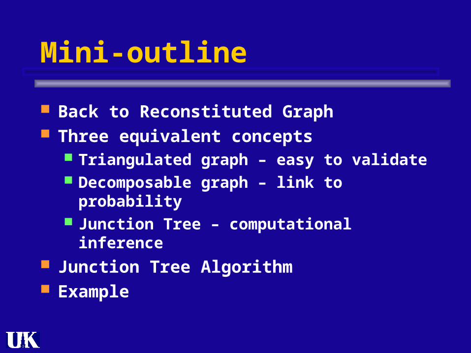
Mini-outline

Back to Reconstituted Graph Three equivalent concepts

Triangulated graph – easy to validate Decomposable graph – link to probability Junction Tree – computational inference

Junction Tree Algorithm Example

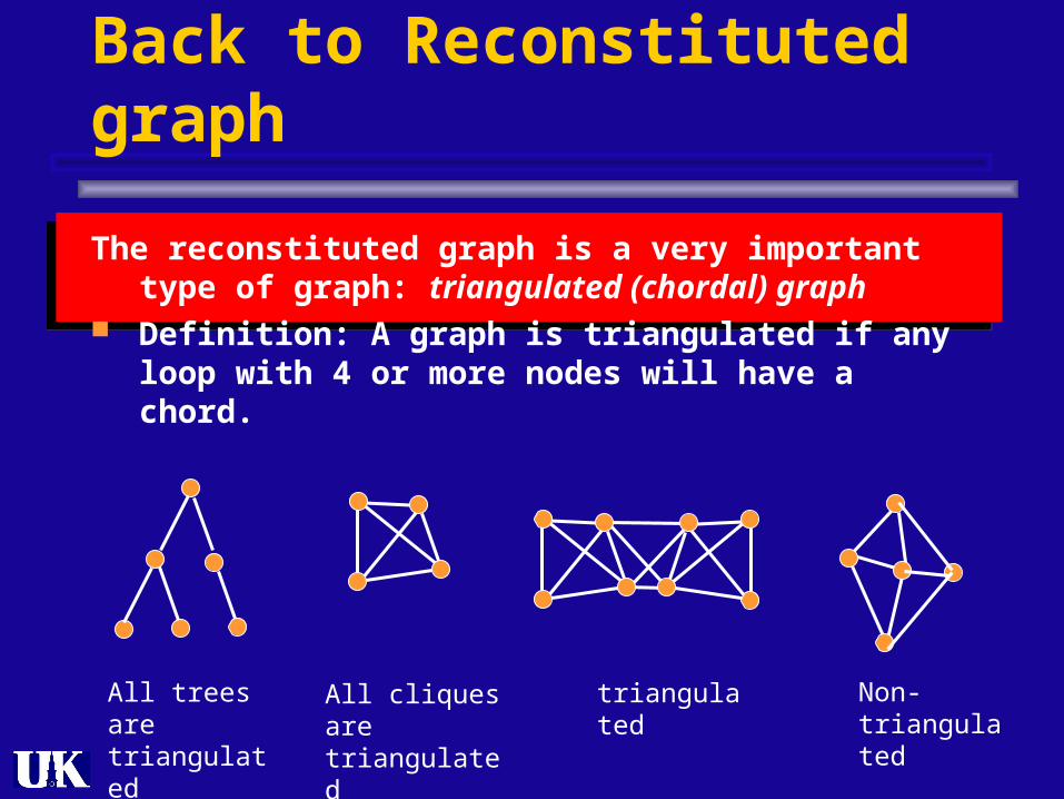
Back to Reconstituted graph

The reconstituted graph is a very important type of graph: triangulated (chordal) graph

Definition: A graph is triangulated if any loop with 4 or more nodes will have a chord.

All trees are triangulated

All cliques are triangulated

triangulated Non-triangulated

v = first node eliminated

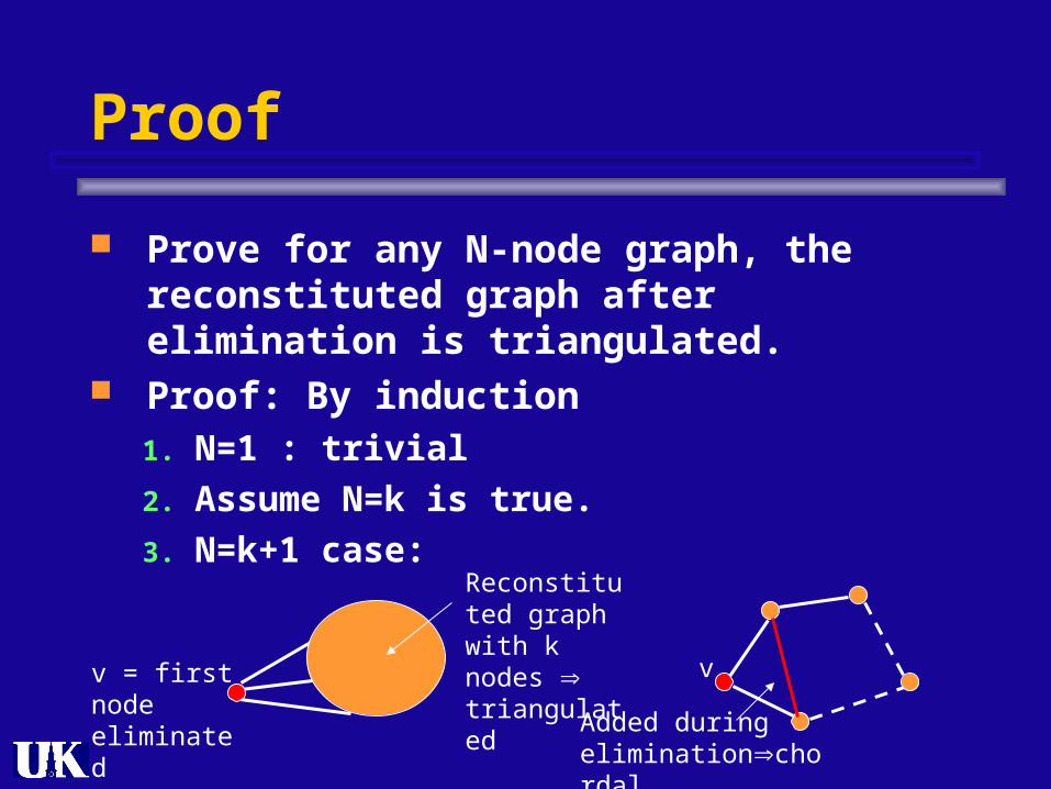
Proof

Prove for any N-node graph, the reconstituted graph after elimination is triangulated.

Proof: By induction1. N=1 : trivial

2. Assume N=k is true.

3. N=k+1 case: Reconstituted graph with k nodes triangulated

Added during eliminationchordal

v

Lessons from graph theory

Graph coloring problem: find the smallest number of vertex colors so that adjacent colors are different = chromatic number

Sample application 1: Scheduling Node = tasks Edge = two tasks are not compatible Coloring = Number of parallel tasks

Sample application 2 : Communication Node = symbols Edge = two symbols may produce the same

output due to transmission error Largest set of vertices with the same color =

number of symbols that can be reliably sent

Lesson from graph theory

Determining the chromatic number is NP-hard Not so for a general type of graph called Perfect

Graph Definition: = the size of the largest clique Triangulated graph is an important type of perfect

graphs. Strong Perfect Graph Conjecture was proved in 2002

(148-page!) Bottom line: Triangulated graph is “algorithmically

friendly” – very easy to check whether a graph is triangulated and to compute properties from such a graph.

Link to Probability: Graph Decomposition

Definition: Given a graph G, a triple (A,B,S) with Vertex(G) = ABS is a decomposition G if 1. S separates A and B (i.e. every path from aA to bB

must past through S.

2. S is a clique Definition: G is decomposable if

1. G is complete or

2. There exist a decomposition (A,B,S) of G such that AS and BS are decomposable.

A BS

What’s the big deal?

Decomposable graph can be parametrized by marginals!

If G is decomposable, then

where C1,C2, …,CN are cliques in G, and S1,S2, …,SN-1 are (special) separators between cliques. Notice there are one less separators than cliques.

Equivalently, we can say that G can parameterized by marginals p(xC) and ratios of marginals, p(xC)/p(xS)

This is not true in general

If the graph can be expressed in terms of a product marginals or ratio of marginals, at least one of the potentials is a marginal.

However, f(XAB) is not a constant

A B

CD

Proof :

Proof by induction:

G can be decomposed into A,B, and S, where AS and B S are decomposable; S separates A and B and is complete.

A BS

All cliques are subsets of either AS or B S

Continue

Recursively apply on AS and BS based on induction assumption.

So what?

TriangulatedGraph

DecomposableGraph

Nice algorithmically Parametrized by marginals

It turns out that

Triangulated Graph Decomposable Graph

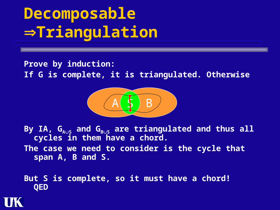
Prove by induction:If G is complete, it is triangulated. Otherwise

By IA, GAS and GBS are triangulated and thus all cycles in them have a chord.

The case we need to consider is the cycle that span A, B and S.

But S is complete, so it must have a chord! QED

Decomposable Triangulation

A BS

TriangulationDecomposable

Prove by induction. Let G be a triangulated graph with N nodes. Show is G can be decomposed into (A,B,S).

If G’s complete, done. If not, choose non-adjacent a and b.

S = smallest set that intersects with all paths between a and b.

A = all nodes in G\S reached by a

B = all nodes in G\S reached by b

Cleary A and B are separated by S.

a bS

BA

TriangulationDecomposable

Need to prove S is complete. Consider arbitrary c,dS.

There is a path acb such that c is the only node in S. If not, then S is not minimum as c can be put into either A or B.

Similarly, there is a path adb. Now we a cycle.

Since G is triangulated, this cycle must have a chord. Since S separates A and B, the chord must be entirely in AS or BS.

Keep shrinking the cycle and eventually there must be a chord between c and d, hence S must be complete.

a bS

c

d

BAa1

b1

a2b2

Recap

Reconstituted graph is triangulated. Triangulated graph = decomposable Joint probability in decomposable graph can

be factorized into marginals and ratios of marginals.

Not very constructive so far: How can we get from LOCAL POTENTIALS to GLOBAL MARGINAL parametrization?

How to get from a local description to a global description?

A decomposable graph (V\S,W\S,S):

At the beginning, we have local representations:

We want

V WS

Message passing

Initialization

Phase 1: Collect

V WS

V WS

(XS)(XS)=1

*(XS)=V\S(XV)

*(XW)= (XW)*(XS)/(XS)*(XS) *(XW)

Why?P(XW) V\S(XW) (XV)/(XS) = (XW)V\S(XV)/(XS) = (XW)*(XS)/(XS) = *(XW)

*(XW)(XV)/*(XS)= [(XW)*(XS)/(XS)](XV)/*(XS) = (XW)(XV)/(XS)= Joint distribution

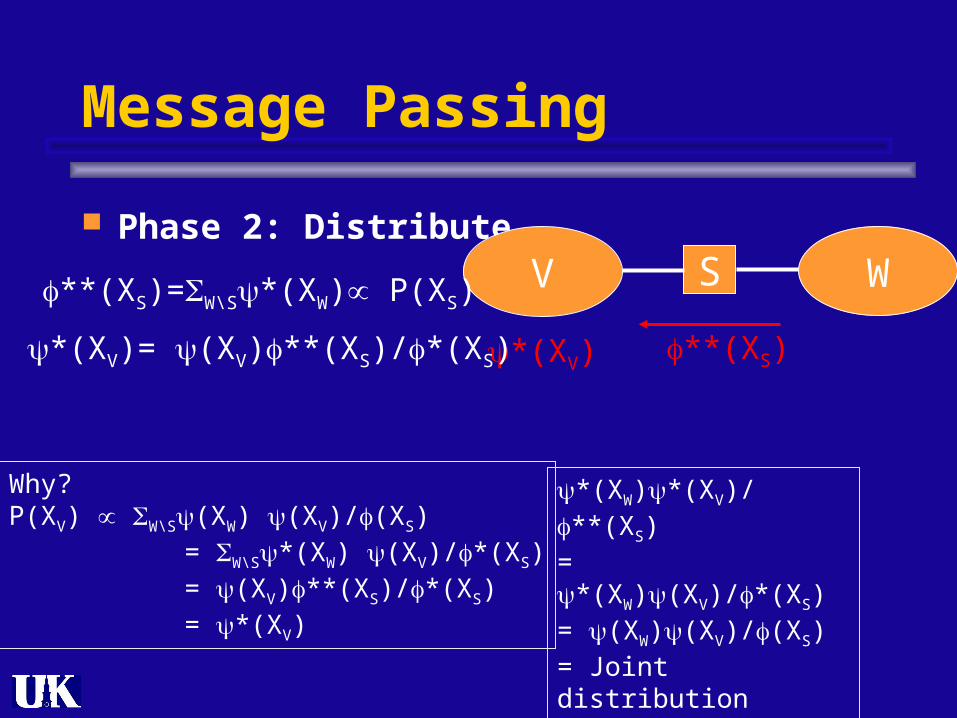
Message Passing

Phase 2: Distribute

V WS

**(XS)*(XV)

**(XS)=W\S*(XW) P(XS)

*(XV)= (XV)**(XS)/*(XS)

Why?P(XV) W\S(XW) (XV)/(XS) = W\S*(XW) (XV)/*(XS) = (XV)**(XS)/*(XS) = *(XV)

*(XW)*(XV)/**(XS)= *(XW)(XV)/*(XS) = (XW)(XV)/(XS)= Joint distribution

Relating Local Description to Message Passing

How to extend message passing to general graph (in terms of cliques)?

To extend the previous message passing algorithm to general graph, we need a recursive decomposition in terms of cliques.

Answer: Junction Tree

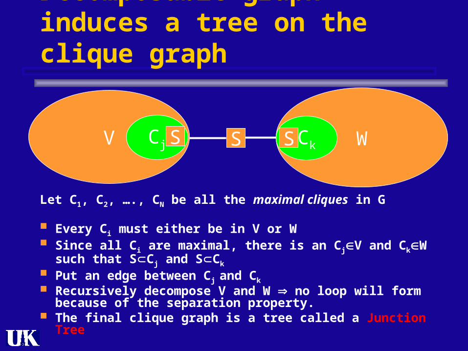
Decomposable graph induces a tree on the clique graph

Let C1, C2, …., CN be all the maximal cliques in G

Every Ci must either be in V or W Since all Ci are maximal, there is an CjV and CkW

such that SCj and SCk Put an edge between Cj and Ck Recursively decompose V and W no loop will form

because of the separation property. The final clique graph is a tree called a Junction Tree

V WSCj CkS S

Properties of a Junction Tree

For any two Ci and Cj, every clique on the unique path on the junction tree between them must contain CiCj

Each branch along the path decompose the graph. So the separator S on the branch must contain CiCj, so

must the clique nodes on either side of the branch Equivalently, for any variable X, all the clique nodes

containing X induces a sub-tree from the junction tree.

Ci CjSA B

Junction Tree Decomposable Graph

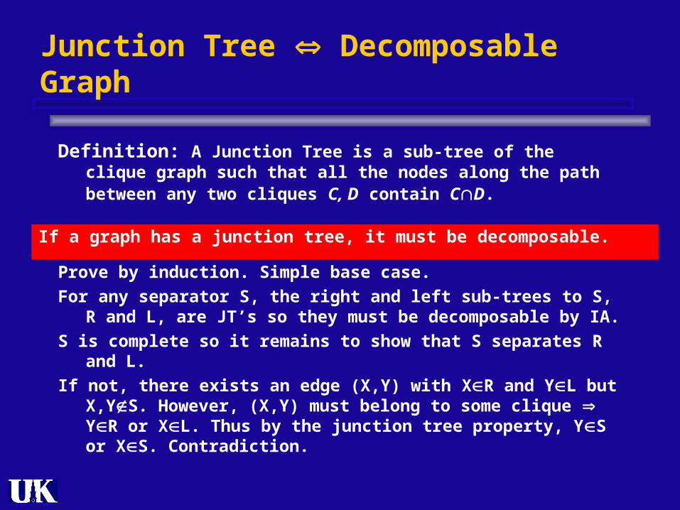
Definition: A Junction Tree is a sub-tree of the clique graph such that all the nodes along the path between any two cliques C, D contain CD.

Prove by induction. Simple base case.

For any separator S, the right and left sub-trees to S, R and L, are JT’s so they must be decomposable by IA.

S is complete so it remains to show that S separates R and L.

If not, there exists an edge (X,Y) with XR and YL but X,YS. However, (X,Y) must belong to some clique YR or XL. Thus by the junction tree property, YS or XS. Contradiction.

If a graph has a junction tree, it must be decomposable.

How to find a junction tree?

Not easy from either definition or decomposition. Define edge weight w(s) = number of variables in

the separator s. Let C1 and C2 be the end clique nodes

Total weight of a junction tree

= X [C1{XC}-1]

= X C1{XC}-N

= C X1{XC}-N

= C |C|-N

Each variable induces a subtree in a junction tree

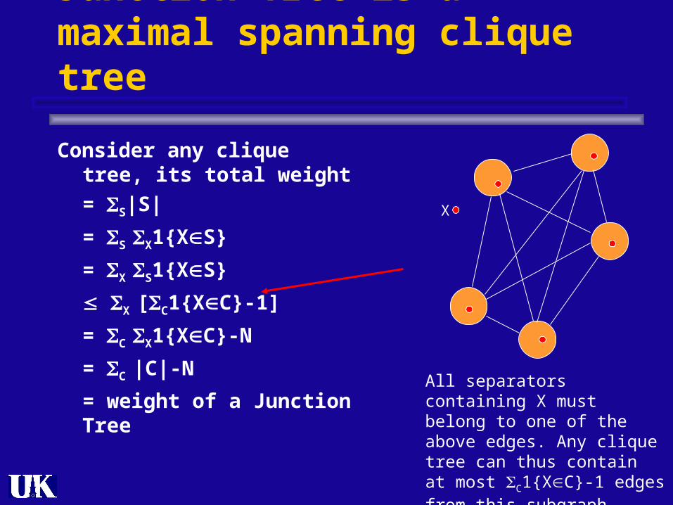
Junction Tree is a maximal spanning clique tree

Consider any clique tree, its total weight

= S|S|

= S X1{XS}

= X S1{XS}

X [C1{XC}-1]

= C X1{XC}-N

= C |C|-N

= weight of a Junction Tree

X

All separators containing X must belong to one of the above edges. Any clique tree can thus contain at most C1{XC}-1 edges from this subgraph.

Example

X2 X3

X1

X4

X5 X6

X7 X8

X9

C1

C3

C2

C6

C4

C5

C1

C3

C2

C6

C4

C5

C3 C4

C1 C2

C6C5

X3

So what? Junction Tree Algorithm

1. Moralize if needed

2. Triangulate using any triangulation algorithm

3. Formulate the clique graph (clique nodes and separator nodes)

4. Compute the junction tree

5. Initialize all separator potentials to be 1.

6. Phase 1: Collect from children

7. Phase 2: Distribute to children

Message from children C: *(XS)=C\S(XC)

Update at parent P: *(XP)= (XP) S *(XS)/(XS)

Message from parent P: **(XP)=P\S**(XP)

Update at child C: *(XC)= (XC) S **(XS)/*(XS)

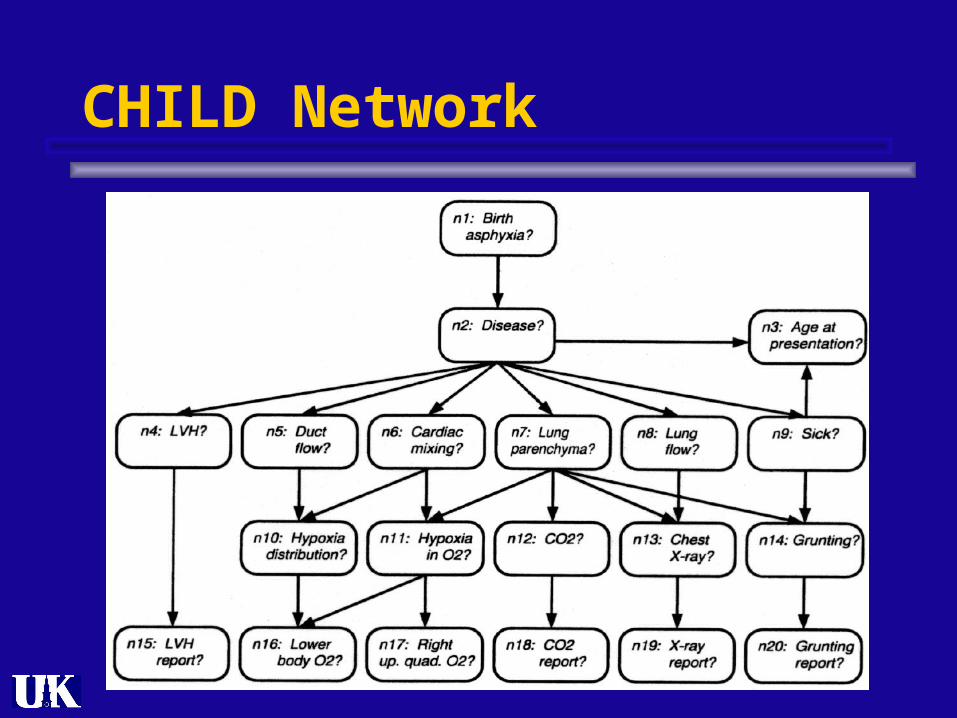
CHILD Network

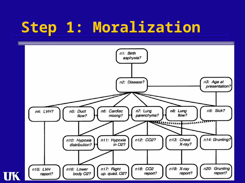
Step 1: Moralization

Step 2: Triangulation

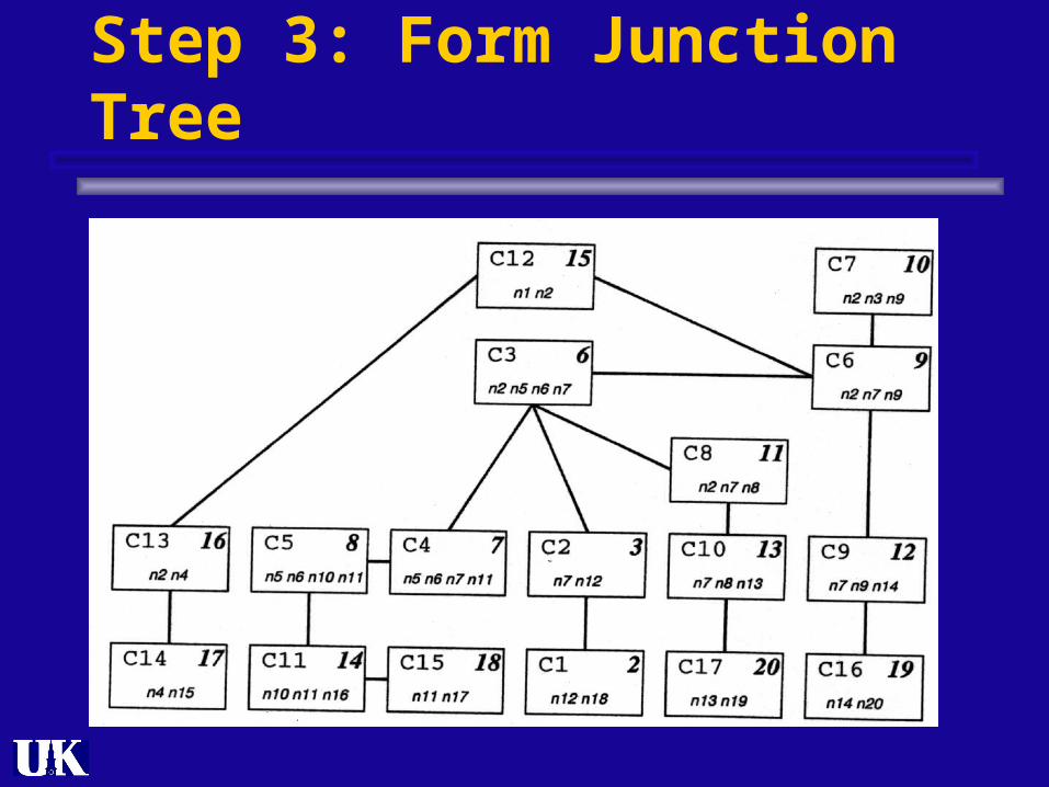
Step 3: Form Junction Tree

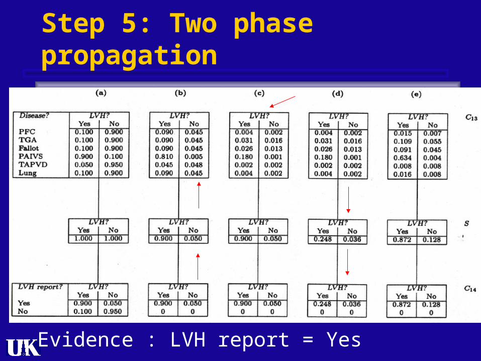
Step 5: Two phase propagation

Evidence : LVH report = Yes

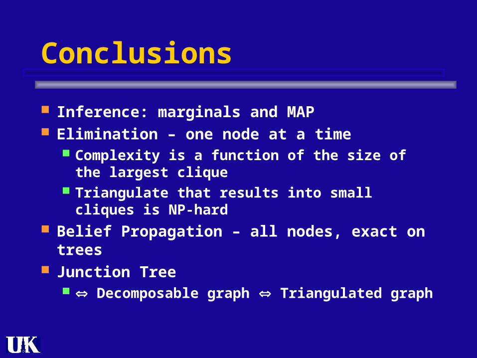
Conclusions

Inference: marginals and MAP Elimination – one node at a time

Complexity is a function of the size of the largest clique

Triangulate that results into small cliques is NP-hard

Belief Propagation – all nodes, exact on trees Junction Tree

Decomposable graph Triangulated graph

Exact Inference on Graphical Models Samson Cheung.

Documents

Transcript of Exact Inference on Graphical Models Samson Cheung.