Exact free Vibration Solutions of Laminated Composite ... · Exact free Vibration Solutions of...

POLITECNICO DI MILANO

Facoltà di Ingegneria IndustrialeCorso di Laurea Magistrale in Ingegneria Spaziale

Exact free Vibration Solutions ofLaminated Composite Plates and

Shells

Relatore: Prof. Lorenzo DOZIO

Studente: Tanzeel ur REHMANMatricola: 781429

Anno Accademico 2015-2016

Contents

List of Figures i

List of Tables ii

Abstract v

Introduction 1

1 Mathematical Modelling 31.1 Exact solutions for cross-ply panels . . . . . . . . . . . . . . . . . 10

1.1.1 Fundamental nuclei for cross-ply panels . . . . . . . . . . . 10

2 Navier Type Solution 13

3 Levy-Type Solution 17

4 Numerical Results 25

Conclusion 31

A Appendix 35

i

List of Figures

1.1 Geometry of the multilayered cylindrical and spherical panels con-sidered in this work and details of the lamination lay-up. . . . . . 4

3.1 Graphical representation of the expansion and assembly procedureto transform the fundamental nuclei of the formulation into thefinal matrices governing the problem. Example of a curved panelwith two layers. . . . . . . . . . . . . . . . . . . . . . . . . . . . . 22

ii

List of Tables

4.1 Sandwich Panel Theory wise comparison . . . . . . . . . . . . . . 264.2 Simply Supported Sandwich with Isotropic Skin Spherical Shell . 264.3 Simply Supported Sandwich with Composite skin Cylindrical Shell 274.4 Single Layer Orthotropic Theory Comparison . . . . . . . . . . . 274.5 Simply Supported Single layered Orthotropic Spherical Shell . . . 284.6 Higher Mode for Isotropic Spherical Shell Comparison with Hashemi’s

Results using ESL4 . . . . . . . . . . . . . . . . . . . . . . . . . . 294.7 ESL3 Calculation for Different Conditions . . . . . . . . . . . . . 294.8 Solution from Khdeir[5] . . . . . . . . . . . . . . . . . . . . . . . . 294.9 Percentage Error of Different Theories . . . . . . . . . . . . . . . 30

A.1 ESL1 Calculation for Different Conditions for Cross Ply LaminatedShells . . . . . . . . . . . . . . . . . . . . . . . . . . . . . . . . . . 35



A.4 LW1 Calculation for Different Conditions for Cross Ply LaminatedShells . . . . . . . . . . . . . . . . . . . . . . . . . . . . . . . . . . 36




iii

Abstract

In this study an Exact free Vibration Solutions of Laminated Composite Shellsis provided based on Carrera’s Approach. This provides with exact solution withdifferent Higher order Shear Deformation Theories by just augmenting the stifnessand mass matrix for a lower order theory. A discussion on Levy type solution ofthe given model establishes the accuracy against different plate solutions. Themodel is then studied on how it can be used to compare the effects of increasingthe order of shear deformation plate theory .

Keywords: Exact free Vibration Solutions of Laminated Composite Shells,Carrera’s Approach, Higher order Shear Deformation Theory, Levy typeSolutions for Shell

v

Introduction

Exact solution of structural elements provides with the basis for early designoptimization, to establish the relationship between different parameters and astandard to rate numerical solutions. Among structural elements unlike beams,plates and shells have exact solution only to certain boundary conditions .

Different theories have been developed over the course of time to findanalytical solutions for plates and then these solutions were extended to shells.Classical Plate Theory [1] (CPT) was developed in 19th century which provedquite suitable for very thin plates but for thicker plates it was required to takeshear deformation with in the plates. This problem was addressed by Mindlin [2]in 20th century in his plate theory (First order Shear Deformation theory FSDT)by modelling the shear deformation within a plate using first order function of theheight of the plate. Some Higher Order Shear Deformation plate Theory (HSDT)developed on FSDT represent the kinematics more accurately.

The theories developed so far were for single plate to move the theory tolaminated plates different concepts were used. They include Equivalent SingleLayer (ESL) theory, Layer Wise (LW) theory and Equivalent Single Layer Zigzag(ESLZ) theory. The basic concept was to link different layers of the laminate inESL all the the layers were represented by a single equivalent layer, in LW thelayers are linked using boundary conditions and ESLZ use the case concept ofESL but with a zigzag function.

Higher order theories provide with more accurate data but at the cost ofhigh computational power. So an optimization is required between computationaltime and accuracy of the result. To do that calculations needed to be done forevery order that meant stiffness and mass matrix calculation for each increasein the order. To make this study less time consuming Carrera [3] came up withstiffness matrices calculation procedure with which to move to a higher order oneonly needed to add a row and a column to already existent matrices for the lowerorder . This concept was used by Dozio [4] to do vibration analysis for certainplate problems. This document discusses the extension of Dozio’s work of plateto shell problem.

The mathematical models developed included differntial equations with

1

two directional variables. To solve these differential equations different solutiontechniques can be used. Two of the solution techniques include Navier type andLevy type solutins. In navier type solution the free harmonic motion includes twosinusoidal functions whereas levy type has only one for each perpendicular direc-tion. Different solution techniques limit the type of problems that can be solvedthat is why Navier and Levy type solution are applicable for different bound-ary conditions and are incapable of providing results for all boundary conditions.This is the reason we do not have analytical solution for all plate problems.

In this study the mathematical model presented in [3] was developed fur-ther to include the effects of curvature so that the problem can be solved forspherical and cylindrical shell in addition to flat plates. After developing themodel,it was solved using navier and Levy type solution technique and the re-sults were compared against 3D exact models for composite, sandwich [7] andsingle layered panel given by Brischetto to establish if the all the geometry, ma-terial properties and plate thickness are explained correctly by the mathematicalmodel. To study the effect of higher modes the results were compared with theresults given by Hashemi [9]. Changing boundary conditions were studied bycomparing modes calculated by Khdeir [5].

Chapter 1 discusses the mathematical modeling of the shell. This chapteradds variables of curvature in two different directions. In Chapter 2 the mathe-matical model is analytical solved using navier type solution and the final resultis given in a mathematical form. Chapter 3 presents the solution of the samemodel using Levy Type solution and the analytical result from this chapter areused in Chapter 4 to do some numerical calculations and the results are com-pared against previously existing results [5].Analysis of the calculation is alsoprovided in this chapter. The last chapter concludes all the discussion with somerecommendations for future work.

2

Chapter 1

Mathematical Modelling

Let’s consider the cylindrical and spherical laminated panels in Figure 1.1, whichare composed of N` layers of homogeneous orthotropic material. Each layer k hasthickness hk and is numbered sequentially from bottom (k = 1) to top (k = N`)of the panel. The total thickness of the panel is h =

∑N`k=1 hk. The undeformed

middle surface Ωk of each layer is described by the two orthogonal curvilinearcoordinates α and β. Let zk denote the rectilinear local thickness coordinate inthe normal direction with respect to Ωk. The components of the displacementfield of layer k are indicated as ukα, ukβ and ukz in the α, β and z directions,respectively.

According to 3-D elasticity and considering curved panels with constantcurvature, the in-plane strains εkp =

εkαα εkββ γkαβ

T of the layer k can beexpressed as a function of the displacement components uk =

ukα ukβ ukz

T

by the following relation:εkp =

(Dk

p + Akp

)uk (1.1)

where

Dkp =

1Hkα

∂∂α

0 0

0 1Hkβ

∂∂β

01Hkβ

∂∂β

1Hkα

∂∂α

0

Akp =

0 0 1HkαR

kα

0 0 1HkβR

kβ

0 0 0

(1.2)

Rkα and Rk

β are the curvature radii of the α and β coordinate curves, respectively,at the generic point of the middle surface Ωk of the layer, and

Hkα = 1 +

zkRkα

Hkβ = 1 +

zkRkβ

(1.3)

It is noted that Hkα = 1 for cylindrical panels since Rk

α = ∞ and Hkα = Hk

β forspherical panels since Rk

α = Rkβ. Note also that when 1/Rk

α = 1/Rkβ = 0, the

above relations degenerate to those for plates.

3

Chapter 1

Figure 1.1: Geometry of the multilayered cylindrical and spherical panels consid-ered in this work and details of the lamination lay-up.

Similarly, the normal strain components εkn =γkαz γkβz εkzz

T can beexpressed as follows

εkn =(Dk

n −Akn + Dk

z

)uk (1.4)

where

Dkn =

0 0 1Hkα

∂∂α

0 0 1Hkβ

∂∂β

0 0 0

Akn =

1

HkαR

kα

0 0

0 1HkβR

kβ

0

0 0 0

(1.5)

and Dkz = ∂

∂zI3.

Assuming a linearly elastic orthotropic material, the constitutive equationsof the kth layer in the laminate reference coordinate system are written as

σkp = Ckppε

kp + Ck

pnεkn

σkn = CkT

pnεkp + Ck

nnεkn

(1.6)

4


where σkp =σkαα σkββ τ kαβ

T is the vector of in-plane stresses, σkn =τ kαz τ kβz σkzz

T

is the vector of normal stresses, and the matrices of stiffness coefficients given by

Ckpp =

Ck11 Ck

12 Ck16

Ck12 Ck

22 Ck26

Ck16 Ck

26 Ck66

Ckpn =

0 0 Ck13

0 0 Ck23

0 0 Ck36

(1.7)

Cknn =

Ck55 Ck

45 0

Ck45 Ck

44 0

0 0 Ck33

(1.8)

are derived from those expressed in the layer reference system through a propercoordinate transformation.

Within the modeling framework proposed by Carrera, an entire class of2-D shell theories can be employed by expressing the displacement vector uk

through the Einstein notation as follows

uk(α, β, ζk, t) = Fτ (ζk)ukτ (α, β, t) (1.9)

where ζk = 2zk/hk is the dimensionless thickness coordinate of the layer (−1 ≤ζk ≤ 1), τ is the theory-related index, Fτ (ζk) are appropriate thickness functionsdefined locally for each layer, and

ukτ (α, β, t) =

ukατ (α, β, t)ukβτ (α, β, t)ukzτ (α, β, t)

(1.10)

is the vector of generalized kinematic coordinates in the assumed displacementmodel corresponding to index τ . Various ESL and LW theories of different order,which is a free parameter of the formulation, can be obtained by choosing thetype of thickness functions and the range values of τ in Eq. (1.9). Both a classof LW theories and a class of ESL theories are implemented in this work. Theyare briefly presented in the following.

A family of LW theories of variable order N is considered by assumingτ = t, r, b (r = 2, . . . , N) and selecting

Ft(ζk) =1 + ζk

2Fr(ζk) = Pr(ζk)− Pr−2(ζk)

Fb(ζk) =1− ζk

2

(1.11)

where Pr(ζk) is the Legendre polynomial of rth order. In so doing, the displace-ment variables ukt and ukb are the actual values at the top and bottom surfaces oflayer k, respectively, and the interlaminar displacement continuity can be easilyimposed as ukt = uk+1

b . Following the nomenclature suggested by Carrera, each

5

Chapter 1

member of this family is here denoted by the acronym LDN , which stands for(L)ayerwise (D)isplacement-based theory of order N . Note that the number ofdegrees of freedom for a LDN theory depends on the number of layers of thelaminated panel and is given by 3(N + 1)N` − 3(N` − 1).

The class of ESL theories considered here involves global thickness functionas increasing power of the global thickness coordinate z, which is measured fromthe middle surface of the curved panel. Since the kinematics is layer-independent,the k index in Eq. (1.9) is dropped. Accordingly,

Ft = 1

Fr = zr (r = 2, . . . , N)

Fb = z

(1.12)

The related N -order member of the ESL family is indicated by EDN , whichstands for (E)quivalent single-layer (D)isplacement-based theory of order N .

Using Eq. (1.9), the geometric relations and constitutive equations of eachlayer of the curved panel are written, respectively, as

εkp =(Dk

p + Akp

)Fτu

kτ εkn =

(Dk

n −Akn + Dk

z

)Fτu

kτ (1.13)

and

σkp = Ckpp

(Dk

p + Akp

)Fsu

ks + Ck

pn

(Dk

n −Akn + Dk

z

)Fsu

ks

σkn = CkT

pn

(Dk

p + Akp

)Fsu

ks + Ck

nn

(Dk

n −Akn + Dk

z

)Fsu

ks

(1.14)

where the index s for the thickness functions in Eq. (1.14) has the same role ofthe index τ .

The equations of motion are here derived from the principle of virtualdisplacements (PVD), which, in absence of any external body and surface force,can be expressed as follows

N∑k=1

∫Ωk

∫Zkδuk

Tρk∂2uk

∂t2HkαH

kβ dz dα dβ

+

N∑k=1

∫Ωk

∫Zk

[δεkp

Tσkp + δεkn

Tσkn

]HkαH

kβ dz dα dβ = 0

(1.15)

where Zk is the layer domain in the thickness direction. Using Eq. (1.9) and thegeometric relations of Eqs. (1.13) into the above PVD statement, the dynamic

6


equilibrium is expressed in weak form by the following equation

N∑k=1

∫Ωk

δukτTρkJkτsαβ

∂2uks∂t2

dα dβ

+

N∑k=1

∫Ωk

∫Zk

[(Dk

pδukτ

)TσkpFτ +

(Dk

nδukτ

)TσknFτ

]HkαH

kβ dz dα dβ

+

N∑k=1

∫Ωk

∫Zk

[δukτ

TAkp

TσkpFτ − δukτ

TAkn

TσknFτ

]HkαH

kβ dz dα dβ

+

N∑k=1

∫Ωk

∫Zkδukτ

TDkz

TσknFτH

kαH

kβ dz dα dβ = 0

(1.16)

whereJkτsαβ =

∫ZkFτFsH

kαH

kβ dz (1.17)

is a thickness integral over the kth layer involving the product of thickness func-tions Fτ and Fs.

After integrating by parts the second term in Eq. (1.16), using the consti-tutive relations (1.14), and exploiting the arbitrariness of the virtual variation ofeach kinematic variable δukτ over Ωk, the following set of differential equations incompact indicial notation is obtained:

Lkτsuks + ρkJkτsαβ

∂2uks∂t2

= 0 (1.18)

where Lkτs is a 3× 3 matrix of differential operators expressed as

Lkτs =

∫Zk

(−Dk

p + Akp

)TCk

pp

(Dk

p + Akp

)+(−Dk

p + Akp

)TCk

pn

(Dk

n −Akn + Dk

z

)+(−Dk

n −Akn + Dk

z

)TCkT

pn

(Dk

p + Akp

)+(−Dk

n −Akn + Dk

z

)TCk

nn

(Dk

n −Akn + Dk

z

)FτFsH

kαH

kβ dz

(1.19)

It is noted that Eq. (1.18) is valid for any index τ and any layer k, andthe summation for repeated index s is implied. Therefore, according to the orderof the assumed shell theory and the number of layers of the curved panel, theexpanded set of governing equations can be derived from Eq. (1.18) for eachspecific case under investigation. However, this set is not written in explicit form,since, according to Carrera’s formulation, Lkτs and ρkJkτsαβ are profitably viewedas invariant entities, which are directly expanded and assembled to build in ahierarchical and automatic manner the matrices of the free vibration problem, as

7

Chapter 1

explained later. For this reason, such entities are called fundamental nuclei ofthe formulation.

Similarly, the arbitrariness of the virtual variation δukτ over the boundaryof the panel yields the following set of boundary conditions

Bkτsuks = 0 (1.20)

where Bkτs is another invariant 3×3 matrix of differential operators called funda-mental nucleus related to the boundary conditions. It is given for Neumann-typeboundary conditions by

Bkτs =

∫Zk

N k

p

TCk

pp

(Dk

p + Akp

)+ N k

p

TCk

pn

(Dk

n −Akn + Dk

z

)+ N k

n

TCkT

pn

(Dk

p + Akp

)+N k

n

TCk

nn

(Dk

n −Akn + Dk

z

)FτFsH

kαH

kβ dz

(1.21)

where N kp and N k

n are matrices containing the components nα and nβ of the unitnormal vector to the boundary as follows

N kp =

nαHkα

0 0

0nβHkβ

0nβHkβ

nαHkα

0

N kn =

0 0 nαHkα

0 0nβHkβ

0 0 0

(1.22)

The fundamental nuclei are presented below in explicit form.

Lkτs11 = Ck55

(Jkτzszαβ +

1

Rkα

2Jkτsβ/α −

1

Rkα

Jkτzsβ − 1

Rkα

Jkτszβ

)− Ck

11Jkτsβ/α

∂2

∂α2− 2Ck

16Jkτs ∂2

∂α∂β− Ck

66Jkτsα/β

∂2

∂β2

Lkτs12 = Ck45

(Jkτzszαβ +

1

RkαR

kβ

Jkτs − 1

Rkα

Jkτszβ − 1

Rkβ

Jkτzsα

)

− (Ck12 + Ck

66)Jkτs∂2

∂α∂β− Ck

16Jkτsβ/α

∂2

∂α2− Ck

26Jkτsα/β

∂2

∂β2

Lkτs13 =

[Ck

55

(Jkτzsβ − 1

Rkα

Jkτsβ/α

)− Ck

11

1

Rkα

Jkτsβ/α − Ck12

1

Rkβ

Jkτs − Ck13J

kτszβ

]∂

∂α

+

[Ck

45

(Jkτzsα − 1

Rkα

Jkτs)− Ck

16

1

Rkα

Jkτs − Ck26

1

Rkβ

Jkτsα/β − Ck36J

kτszα

]∂

∂β

8


Lkτs21 = Ck45

(Jkτzszαβ +

1

RkαR

kβ

Jkτs − 1

Rkα

Jkτzsβ − 1

Rkβ

Jkτszα

)

− (Ck12 + Ck

66)Jkτs∂2

∂α∂β− Ck

16Jkτsβ/α

∂2

∂α2− Ck

26Jkτsα/β

∂2

∂β2

Lkτs22 = Ck44

(Jkτzszαβ +

1

Rkβ

2Jkτsα/β −

1

Rkβ

Jkτzsα − 1

Rkβ

Jkτszα

)

− Ck22J

kτsα/β

∂2

∂β2− 2Ck

26Jkτs ∂2

∂α∂β− Ck

66Jkτsβ/α

∂2

∂α2

Lkτs23 =

[Ck

45

(Jkτzsβ − 1

Rkβ

Jkτs

)− Ck

16

1

Rkα

Jkτsβ/α − Ck26

1

Rkβ

Jkτs − Ck36J

kτszβ

]∂

∂α

+

[Ck

44

(Jkτzsα − 1

Rkβ

Jkτsα/β

)− Ck

12

1

Rkα

Jkτs − Ck22

1

Rkβ


kτszα

]∂

∂β

Lkτs31 =

[Ck

11

1

Rkα

Jkτsβ/α + Ck12

1

Rkβ

Jkτs + Ck55

(1

Rkα

Jkτsβ/α − Jkτszβ

)+ Ck

13Jkτzsβ

]∂

∂α

+

[Ck

16

1

Rkα

Jkτs + Ck26

1

Rkβ

Jkτsα/β + Ck36J

kτzsα + Ck

45

(1

Rkα

Jkτs − Jkτszα

)]∂

∂β

Lkτs32 =

[Ck

16

Rkα

Jkτsβ/α +Ck

26

Rkβ

Jkτs + Ck45

(1

Rkβ

Jkτs − Jkτszβ

)+ Ck

36Jkτzsβ

]∂

∂α

+

[Ck

12

Rkα

Jkτs +Ck

22

Rkβ

Jkτsα/β + Ck23J

kτzsα + Ck

44

(1

Rkβ

Jkτsα/β − Jkτszα

)]∂

∂β

Lkτs33 =

[Ck

33Jkτzszαβ +

1

Rkα

(Ck

11

Rkα

Jkτsβ/α + 2Ck

12

Rkβ

Jkτs + Ck13J

kτszβ + Ck

13Jkτzsβ

)

+1

Rkβ

(Ck

22

1

Rkβ

Jkτsα/β + Ck23J

kτszα + Ck

23Jkτzsα

)]

− Ck55J

kτsβ/α

∂2

∂α2− 2Ck

45Jkτs ∂2

∂α∂β− Ck

44Jkτsα/β

∂2

∂β2

Bkτs11 = nα

[Ck

11Jkτsβ/α

∂

∂α+ Ck

16Jkτs ∂

∂β

]+ nβ

[Ck

16Jkτs ∂

∂α+ Ck

66Jkτsα/β

∂

∂β

]

Bkτs12 = nα

[Ck

16Jkτsβ/α

∂

∂α+ Ck

12Jkτs ∂

∂β

]+ nβ

[Ck

66Jkτs ∂

∂α+ Ck

26Jkτsα/β

∂

∂β

]

9

Chapter 1

Bkτs13 = nα

[1

Rkα

Ck11J

kτsβ/α +

1

Rkβ

Ck12J

kτs + Ck13J

kτszβ

]

+ nβ

[1

Rkα

Ck16J

kτs +1

Rkβ

Ck26J

kτsα/β + Ck

36Jkτszα

]

Bkτs21 = nα

[Ck

16Jkτsβ/α

∂

∂α+ Ck

66Jkτs ∂

∂β

]+ nβ

[Ck

12Jkτs ∂

∂α+ Ck

26Jkτsα/β

∂

∂β

]Bkτs22 = nα

[Ck

66Jkτsβ/α

∂

∂α+ Ck

26Jkτs ∂

∂β

]+ nβ

[Ck

26Jkτs ∂

∂α+ Ck

22Jkτsα/β

∂

∂β

]

Bkτs23 = nα

[1

Rkα

Ck16J

kτsβ/α +

1

Rkβ

Ck26J

kτs + Ck36J

kτszβ

]

+ nβ

[1

Rkα

Ck12J

kτs +1

Rkβ

Ck22J

kτsα/β + Ck

23Jkτszα

]

Bkτs31 = nα

[Ck

55Jkτszβ − 1

Rkα

Ck55J

kτsβ/α

]+ nβ

[Ck

45Jkτszα − 1

Rkα

Ck45J

kτs

]

Bkτs32 = nα

[Ck

45Jkτszβ − 1

Rkβ

Ck45J

kτs

]+ nβ

[Ck

44Jkτszα − 1

Rkβ

Ck44J

kτsα/β

]

Bkτs33 = nα

[Ck

55Jkτsβ/α

∂

∂α+ Ck

45Jkτs ∂

∂β

]+ nβ

[Ck

45Jkτs ∂

∂α+ Ck

44Jkτsα/β

∂

∂β

]

1.1 Exact solutions for cross-ply panels

The boundary value problem derived above, in the most general case of arbitraryboundary conditions and lamination lay-ups, could be solved only by implement-ing approximate procedures. Exact solutions are available for special cases inwhich the shell panel is at least simply-supported along two opposite edges andthe material has the following properties (as it is the case of cross-ply laminates):

Ck16 = Ck

26 = Ck36 = Ck

45 (1.23)

1.1.1 Fundamental nuclei for cross-ply panels

The fundamental nuclei of cross-ply cylindrical and spherical shell panels reduceto the following expressions:

Lkτs11 = Ck55

(Jkτzszαβ +

1

Rkα

2Jkτsβ/α −

1

Rkα

Jkτzsβ − 1

Rkα

Jkτszβ

)− Ck

11Jkτsβ/α

∂2

∂α2− Ck

66Jkτsα/β

∂2

∂β2

10


Lkτs12 = −(Ck12 + Ck

66)Jkτs∂2

∂α∂β

Lkτs13 =

[Ck

55

(Jkτzsβ − 1

Rkα

Jkτsβ/α

)− Ck

11

1

Rkα

Jkτsβ/α − Ck12

1

Rkβ

Jkτs − Ck13J

kτszβ

]∂

∂α

Lkτs21 = −(Ck12 + Ck

66)Jkτs∂2

∂α∂β

Lkτs22 = Ck44

(Jkτzszαβ +

1

Rkβ

2Jkτsα/β −

1

Rkβ

Jkτzsα − 1

Rkβ

Jkτszα

)− Ck

22Jkτsα/β

∂2

∂β2− Ck

66Jkτsβ/α

∂2

∂α2

Lkτs23 =

[Ck

44

(Jkτzsα − 1

Rkβ

Jkτsα/β

)− Ck

12

1

Rkα

Jkτs − Ck22

1

Rkβ


kτszα

]∂

∂β

Lkτs31 =

[Ck

11

1

Rkα

Jkτsβ/α + Ck12

1

Rkβ

Jkτs + Ck55

(1

Rkα

Jkτsβ/α − Jkτszβ

)+ Ck

13Jkτzsβ

]∂

∂α

Lkτs32 =

[Ck

12

Rkα

Jkτs +Ck

22

Rkβ

Jkτsα/β + Ck23J

kτzsα + Ck

44

(1

Rkβ

Jkτsα/β − Jkτszα

)]∂

∂β

Lkτs33 =

[Ck

33Jkτzszαβ +

1

Rkα

(Ck

11

Rkα

Jkτsβ/α + 2Ck

12

Rkβ

Jkτs + Ck13J

kτszβ + Ck

13Jkτzsβ

)

+1

Rkβ

(Ck

22

1

Rkβ

Jkτsα/β + Ck23J

kτszα + Ck

23Jkτzsα

)]− Ck

55Jkτsβ/α

∂2

∂α2− Ck

44Jkτsα/β

∂2

∂β2

and

Bkτs11 = nα

[Ck

11Jkτsβ/α

∂

∂α

]+ nβ

[Ck

66Jkτsα/β

∂

∂β

]

Bkτs12 = nα

[Ck

12Jkτs ∂

∂β

]+ nβ

[Ck

66Jkτs ∂

∂α

]

Bkτs13 = nα

[1

Rkα

Ck11J

kτsβ/α +

1

Rkβ

Ck12J

kτs + Ck13J

kτszβ

]

Bkτs21 = nα

[Ck

66Jkτs ∂

∂β

]+ nβ

[Ck

12Jkτs ∂

∂α

]Bkτs22 = nα

[Ck

66Jkτsβ/α

∂

∂α

]+ nβ

[Ck

22Jkτsα/β

∂

∂β

]

Bkτs23 = nβ

[1

Rkα

Ck12J

kτs +1

Rkβ

Ck22J

kτsα/β + Ck

23Jkτszα

]

Bkτs31 = nα

[Ck

55Jkτszβ − 1

Rkα

Ck55J

kτsβ/α

]

11

Chapter 1

Bkτs32 = nβ

[Ck

44Jkτszα − 1

Rkβ

Ck44J

kτsα/β

]

Bkτs33 = nα

[Ck

55Jkτsβ/α

∂

∂α

]+ nβ

[Ck

44Jkτsα/β

∂

∂β

]In particular, the boundary conditions along each edge are given explicitly asfollows:

– along α = 0, a :

ukαs = 0 or Ck11J

kτsβ/α

∂ukαs∂α

+ Ck12J

kτs∂ukβs∂β

+

[1

Rkα

Ck11J

kτsβ/α +

1

Rkβ

Ck12J

kτs + Ck13J

kτszβ

]ukzs = 0

ukβs = 0 or Ck66J

kτs∂ukαs

∂β+ Ck

66Jkτsβ/α

∂ukβs∂α

= 0

ukzs = 0 or[Ck

55Jkτszβ − 1

Rkα

Ck55J

kτsβ/α

]ukαs + Ck

55Jkτsβ/α

∂ukzs∂α

= 0

(1.24)

– along β = 0, b :

ukαs = 0 or Ck66J

kτsα/β

∂ukαs∂β

+ Ck66J

kτs∂ukβs∂α

= 0

ukβs = 0 or Ck12J

kτs∂ukαs

∂α+ Ck

22Jkτsα/β

∂ukβs∂β

+

[1

Rkα

Ck12J

kτs +1

Rkβ

Ck22J

kτsα/β + Ck

23Jkτszα

]ukzs = 0

ukzs = 0 or

[Ck

44Jkτszα − 1

Rkβ

Ck44J

kτsα/β

]ukβs + Ck

44Jkτsα/β

∂ukzs∂β

= 0

(1.25)

12

Chapter 2

Navier Type Solution

Exact Navier-type solutions are available for a special case in which the panel isfully simply-supported. According to the theoretical framework outlined in theprevious section, the condition of simple support along edges α = 0, a is specifiedherein for any index s as

(along α = 0, a)

Ck11J

kτsβ/α

∂ukαs∂α

+ Ck12J

kτs∂ukβs∂β

+

[1

Rkα

Ck11J

kτsβ/α +

1

Rkβ

Ck12J

kτs + Ck13J

kτszβ

]ukzs = 0

ukβs = 0

ukzs = 0

(2.1)

Simply-supported edges along β = 0, b correspond to the following boundaryconditions

(along β = 0, b)

ukαs = 0

Ck12J

kτs∂ukαs

∂α+ Ck

22Jkτsα/β

∂ukβs∂β

+

[1

Rkα

Ck12J

kτs +1

Rkβ

Ck22J

kτsα/β + Ck

23Jkτszα

]ukzs = 0

ukzs = 0

(2.2)

A solution for free harmonic motion of the laminate which satisfies the aboveboundary conditions is sought as follows

uks =

ukαsukβsukzs

=

ukαsmn cos(αmα) sin (βnβ)ukβsmn sin(αmα) cos (βnβ)ukzsmn sin(αmα) sin (βnβ)

ejωmnt (2.3)

13

Chapter 2

where ukαsmn, ukβsmn and ukzsmn are the amplitude of the harmonic motion, ωmndenotes the unknown eigenfrequency associated with the (m,n)-th eigenmode(m,n = 0, 1, 2, . . . ) and

αm =mπ

a(2.4)

βn =nπ

b(2.5)

m and n are the number of half-waves in x and y directions, respectively. Sub-stituting Eq. (2.3) into Eq. (1.18), the corresponding eigenvalue problem isexpressed as follows

[Kkτs − ω2

mnMkτs]uksmn = 0 (2.6)

where

uksmn =

ukαsmnukβsmnukzsmn

(2.7)

and the 3× 3 matrices Kkτs and Mkτs are called stiffness and mass fundamentalnuclei of the formulation corresponding to a Navier-type free vibration solution.

14

Navier Type Solution

The elements of the stiffness nucleus are given by

Kkτs11 = α2

mCk11J

kτsβ/α + β2

nCk66J

kτsα/β + Ck

55Jkτzszαβ

+ Ck55

(1

Rkα

2Jkτsβ/α −

1

Rkα

Jkτzsβ − 1

Rkα

Jkτszβ

)Kkτs

12 = αmβn(Ck12 + Ck

66)Jkτs

Kkτs13 = αm

(Ck

55Jkτzsβ − Ck

13Jkτszβ

)− αm

(Ck

55

1

Rkα

Jkτsβ/α + Ck11

1

Rkα

Jkτsβ/α + Ck12

1

Rkβ

Jkτs

)Kkτs

21 = αmβn(Ck12 + Ck

66)Jkτs

Kkτs22 = β2

nCk22J

kτsα/β + α2

mCk66J

kτsβ/α + Ck

44Jkτzszαβ

+ Ck44

(1

Rkβ

2Jkτsα/β −

1

Rkβ

Jkτzsα − 1

Rkβ

Jkτszα

)Kkτs

23 = βn

(Ck

44Jkτzsα − Ck

23Jkτszα

)− βn

(Ck

44

1

Rkβ

Jkτsα/β + Ck12

1

Rkα

Jkτs + Ck22

1

Rkβ

Jkτsα/β

)Kkτs

31 = αm

(Ck

55Jkτszβ − Ck

13Jkτzsβ

)− αm

(Ck

11

1

Rkα

Jkτsβ/α + Ck12

1

Rkβ

Jkτs + Ck55

1

Rkα

Jkτsβ/α

)Kkτs

32 = βn

(Ck

44Jkτszα − Ck

23Jkτzsα

)− βn

(Ck

12

1

Rkα

Jkτs + Ck22

1

Rkβ

Jkτsα/β + Ck44

1

Rkβ

Jkτsα/β

)Kkτs

33 = α2nC

k55J

kτsβ/α + β2

nCk44J

kτsα/β + Ck

33Jkτzszαβ

+

[1

Rkα

(Ck

11

1

Rkα

Jkτsβ/α + 2Ck12

1

Rkβ

Jkτs + Ck13J

kτszβ + Ck

13Jkτzsβ

)

+1

Rkβ

(Ck

22

1

Rkβ

Jkτsα/β + Ck23J

kτszα + Ck

23Jkτzsα

)]

The elements of the mass nucleus are given by

Mkτs11 = Mkτs

22 = Mkτs33 = ρkJkτsαβ

Mkτs12 = Mkτs

13 = Mkτs21 = Mkτs

23 = Mkτs31 = Mkτs

32 = 0

15

Chapter 2

16

Chapter 3

Levy-Type Solution

Exact Levy-type solutions are available for a special case in which the panel issimply-supported along two opposite edges, whereas the other two edges can besimply-supported, clamped or free.

Let’s consider the case where the edges β = 0, b of the shell panel areassumed to be simply supported. According to the theoretical framework outlinedin the previous section, the condition of simple support along edges β = 0, b isspecified herein for any index s as

(along β = 0, b)

ukαs = 0

Ck12J

kτs∂ukαs

∂α+ Ck

22Jkτsα/β

∂ukβs∂β

+

[1

Rkα

Ck12J

kτs +1

Rkβ

Ck22J

kτsα/β + Ck

23Jkτszα

]ukzs = 0

ukzs = 0

(3.1)

A solution for free harmonic motion of the laminate which satisfies the aboveboundary conditions is sought as follows

uks =

ukαsukβsukzs

=

ukαsp(α) sin (βpβ)ukβsp(α) cos (βpβ)ukzsp(α) sin (βpβ)

ejωpt (p = 1, 2, . . . ) (3.2)

where ωp denotes the unknown eigenfrequency associated with the p-th eigenmodeand βp = pπ/b. Note that the expression in Eq. (3.2) is indeed a series solutionwith respect to index p due to the same Einstein notation used before for theory-related indices.

Substituting Eq. (3.2) into Eq. (1.18) yields, for each p = 1, 2, . . . , the

17

Chapter 3

following system of second-order ordinary differential equations

Lkτs2

d2Uks

dα2− Lkτs1

dUks

dα− Lkτs0 Uk

s = 0 (3.3)

where

Uks(α) =

ukαsp(α)ukβsp(α)ukzsp(α)

(3.4)

is the vector of unknown amplitudes and

Lkτs2 = Jkτsβ/α

Ck11 0 0

0 Ck66 0

0 0 Ck55

(3.5)

Lkτs1 =

0 l12 l13

l21 0 0l31 0 0

(3.6)

Lkτs0 =

l11 0 00 l22 l23

0 l32 l33

(3.7)

are the 3×3 matrices representing the fundamental nuclei of the governing equa-

18

Levy-Type Solution

tions along α direction. The elements of the L matrices are given by

l11 = β2pC

k66J

kτsα/β + Ck

55Jkτzszαβ − ρkJkτsαβ ω

2p

+ Ck55

(1

Rkα

2Jkτsβ/α −

1

Rkα

Jkτzsβ − 1

Rkα

Jkτszβ

)l12 = βp

(Ck

12 + Ck66

)Jkτs

l13 = Ck55J

kτzsβ − Ck

13Jkτszβ − Ck

55

1

Rkα

Jkτsβ/α − Ck11

1

Rkα

Jkτsβ/α − Ck12

1

Rkβ

Jkτs

l21 = −βp(Ck

12 + Ck66

)Jkτs

l22 = β2pC

k22J

kτsα/β + Ck


2p

+ Ck44

(1

Rkβ

2Jkτsα/β −

1

Rkβ

Jkτzsα − 1

Rkβ

Jkτszα

)l23 = βp

(Ck

44Jkτzsα − Ck

23Jkτszα

)− βp

(Ck

44

1

Rkβ

Jkτsα/β + Ck12

1

Rkα

Jkτs + Ck22

1

Rkβ

Jkτsα/β

)l31 = Ck

13Jkτzsβ − Ck

55Jkτszβ + Ck

55

1

Rkα

Jkτsβ/α + Ck11

1

Rkα

Jkτsβ/α + Ck12

1

Rkβ

Jkτs

l32 = βp

(Ck

44Jkτszα − Ck

23Jkτzsα

)− βp

(Ck

44

1

Rkβ

Jkτsα/β + Ck12

1

Rkα

Jkτs + Ck22

1

Rkβ

Jkτsα/β

)l33 = β2

pCk44J

kτsα/β + Ck


2p

+

[1

Rkα

(Ck

11

1

Rkα

Jkτsβ/α + 2Ck12

1

Rkβ

Jkτs + Ck13J

kτszβ + Ck

13Jkτzsβ

)

+1

Rkβ

(Ck

22

1

Rkβ

Jkτsα/β + Ck23J

kτszα + Ck

23Jkτzsα

)]

Along edges α = 0, a we can have

– clamped conditions:

ukαs = 0

ukβs = 0

ukzs = 0

(3.8)

19

Chapter 3

– free conditions:

Ck11J

kτsβ/α

∂ukαs∂α

+ Ck12J

kτs∂ukβs∂β

+

[1

Rkα

Ck11J

kτsβ/α +

1

Rkβ

Ck12J

kτs + Ck13J

kτszβ

]ukzs = 0

Ck66J

kτs∂ukαs

∂β+ Ck

66Jkτsβ/α

∂ukβs∂α

= 0[Ck

55Jkτszβ − 1

Rkα

Ck55J

kτsβ/α

]ukαs + Ck

55Jkτsβ/α

∂ukzs∂α

= 0

(3.9)

– simply-supported conditions:

Ck11J

kτsβ/α

∂ukαs∂α

+ Ck12J

kτs∂ukβs∂β

+

[1

Rkα

Ck11J

kτsβ/α +

1

Rkβ

Ck12J

kτs + Ck13J

kτszβ

]ukzs = 0

ukβs = 0

ukzs = 0

(3.10)

Substituting Eq. (3.2) into the above boundary conditions yields, for each p =1, 2, . . . , the following equations for each layer k

Bkτs1

dUks

dα+ Bkτs

0 Uks = 0 (α = 0, a) (3.11)

where Bkτsi (i = 0, 1) is the 3 × 3 fundamental nucleus corresponding to the

boundary conditions. According to the type of edge condition at α = 0, a, theboundary-related nuclei are expressed as follows

– clamped edge:

Bkτs1 =

0 0 00 0 00 0 0

Bkτs

0 =

δτs 0 00 δτs 00 0 δτs

20

Levy-Type Solution

– free edge:

Bkτs1 = Jkτsβ/α

Ck11 0 0

0 Ck66 0

0 0 Ck55

Bkτs

0 =

0 −βpCk12J

kτs Ck13J

kτszβ + 1

RkαCk

11Jkτsβ/α + 1

RkβCk

12Jkτs

βpCk66J

kτs 0 0

Ck55J

kτszβ − 1

RkαCk

55Jkτsβ/α 0 0

– simply-supported edge:

Bkτs1 = Jkτsβ/α

Ck11 0 00 0 00 0 0

Bkτs

0 =

0 −βpCk12J

kτs Ck

13Jkτszβ + 1

RkαCk

11Jkτsβ/α + 1

RkβCk

12Jkτs

0 δτs 00 0 δτs

Equations (3.3) and (3.11) are written at layer level in terms of fundamental nucleiLkτsi and Bkτs

i . In order to obtain the governing equations and related boundaryconditions of the multilayered plate according to the assumed kinematic theory,a simple expansion and assembly-like procedure is applied. The procedure isgraphically depicted in Figure 3.1 for L matrices.

First, by varying the theory-related indices τ and s over the defined ranges,the nuclei Lkτsi and Bkτs

i are expanded so that a new system of equations andrelated boundary conditions is obtained as follows

Lk2d2Uk

dα2− Lk1

dUk

dα− Lk0U

k = 0

Bk1

dUk

dα+ Bk

0Uk = 0 (α = 0, a)

(3.12)

whereUk(x) =

[UkT

t (α) UkT

r (α) UkT

b (α)]T

(3.13)

and

Lki =

Lktti Lktri LktbiLkrti Lkrri Lkrbi

Lkbti Lkbri Lkbbi

, Bki =

Bktti Bktr

i Bktbi

Bkrti Bkrr

i Bkrbi

Bkbti Bkbr

i Bkbbi

(3.14)

Note that Lki and Bki are square matrices of dimension 3(N + 1).

21

Chapter 3

Figure 3.1: Graphical representation of the expansion and assembly procedureto transform the fundamental nuclei of the formulation into the final matricesgoverning the problem. Example of a curved panel with two layers.

Then, the final set of equations is written as

L2d2U

dα2− L1

dU

dα− L0U = 0

B1dU

dα+ B0U = 0 (α = 0, a)

(3.15)

where U(α) is the vector containing all the independent kinematic variablesUk(α) (k = 1, . . . , N`), and the resulting matrices Li and Bi are simply summedlayer-by-layer in case of ESL theories or assembled by enforcing the interlaminarcontinuity condition in case of LW theories.

A state space approach is used to solve the free vibration problem byconverting Eqs. (3.15) into a first-order form as follows

dZ

dα= AZ

BZ = 0 (α = 0, a)(3.16)

22

Levy-Type Solution

whereZ(α) =

dU/dα

U

(3.17)

and

A =

[L2 00 I

]−1 [L1 L0

I 0

], B =

[B1 B0

](3.18)

A general solution can be expressed as

Z(α) = eAαc (3.19)

where c is a vector of constants connected to boundary conditions. Using aspectral decomposition of the exponential matrix, the solution can be written as

Z(α) = VDiag(eλiα

)V−1c (3.20)

where V is the matrix of eigenvectors of A and λi are the corresponding eigen-values. Replacement of solution (3.20) into the system of boundary equations inEq. (3.16) yields a homogeneous system

BVDiag(eλiα

)V−1c = Hc = 0 (α = 0, a) (3.21)

The natural frequencies associated with the p-th mode are determined by setting|H| = 0. Note that, since H = H(ωp), an iterative numerical procedure must beemployed to derive the frequency parameters.

As a summary, the present method was implemented through the followingsteps:

1. Select the number of half waves p of the vibration mode in the β direction.

2. Build the fundamental nuclei Bkτsi (i = 0, 1) using Eqs. (3-3) according to

the edge condition at α = 0 and α = a.

3. Expand the nuclei Bkτsi as outlined in Figure 3.1 in order to build Bi ma-

trices and the related B matrix in Eq. (3.18).

4. For any iteration step over the selected range values of ωp:

(a) Build the fundamental nuclei Lkτsi (i = 0, 1, 2).

(b) Expand the nuclei Lkτsi as outlined in Figure 3.1 in order to build Limatrices and compute A matrix in Eq. (3.18).

(c) Compute the spectral decomposition of matrix A.

(d) Compute the H matrix in Eq. (3.21) and its determinant.

(e) Check if the determinant changes sign. If yes, the value of the naturalfrequency is found by using the bisection method.

23

Chapter 3

24

Chapter 4

Numerical Results

Each eigen value problem was solved using bisection method. During the calcu-lation of cylindrical shell the radius of curvature in one direction was taken to beinfinite. Care was taken that the correct direction for infinite radius was chosen.For each case the calculations were checked by putting both the radii as infiniteand then comparing the results with the results of a flat plate (As a flat plate isa sphere with both the radii as infinite.

Different theories were used for calculations and the materials used forPVC material used as foam core for sandwich panels and isotropic spherical shellhad Young modulus E = 180MPa, Poisson ratio ν = 0.37 and mass density ρ =50kg/m3. The isotropic aluminum alloy Al2024 used as skins had Young modulusE = 73GPa, Poisson ratio ν = 0.3 and mass density ρ = 2800kg/m3. Theorthotropic layers in Gr/Ep for composite skins and Single layered OrthotropicSpherical Shell had Young moduli E1 = 132.38GPa and E2 = E3 = 10.756GPa,shear moduli G12 = G13 = 5.6537GPa and G23 = 3.603GPa, Poisson ratiosν12 = ν13 = 0.24 and ν23 = 0.49, the mass density is ρ = 1600kg/m3. Andfor the laminated composites each layer had E1 = 25GPa,E2 = E3 = 1GPa,ν = 0.25,and G = 0.2 ∗ E2

These calculations for simply supported sandwich with isotropic skin spher-ical shells were carried out with different theories for thick shells as shown in table4.1.It can be seen that the error for an equivalent single layer theory for a verythin shell is very high where as the error for layer wise theory is small and de-creases with an increase in order of LW theory, also it can be seen that the changein Percentage error from Brischetto’s results becomes negligible as the order ofthe theory is increased from LW3. More accurate results given by LW theoriesfor sandwich panel is more consistent as LW theories define the properties foreach layer whereas in ESL all the material is represented by a single layer. Theadvantage ESL has over LW is lesser computational power but the loss in accu-racy was too much so we had to compensate and LW3 was selected as the bestoption for further analysis of sandwich panels in 4.2 and 4.3 .

25

Chapter 4

Brischetto[7] ED4 % error LD1 % error LD2 % error LD3 % error LD4 % errorp=1 1.463 2.755 88.284 1.480 1.189 1.461 0.123 1.461 0.123 1.461 0.123

2.550 5.249 105.848 2.675 4.895 2.522 1.094 2.521 1.126 2.521 1.126p=2 3.064 4.583 49.590 3.098 1.126 3.071 0.232 3.071 0.232 3.071 0.232

3.108 6.775 117.982 3.262 4.948 3.084 0.769 3.083 0.808 3.083 0.808

Table 4.1: Sandwich Panel Theory wise comparison

LW3 Brischetto[7] Percentage errorr/h=5 p=1 1.461 1.463 0.123

2.521 2.550 1.126p=2 3.071 3.064 0.232

3.083 3.108 0.808r/h=10 p=1 2.761 2.756 0.174

3.963 3.969 0.154p=2 4.933 4.954 0.416

5.949 5.941 0.131r/h=100 p=1 17.307 17.298 0.049

22.351 22.345 0.026p=2 29.508 29.488 0.068

54.883 54.875 0.015r/h=1000 p=1 70.378 70.375 0.004

218.892 218.880 0.005p=2 229.388 229.380 0.004

543.303 543.310 0.001

Table 4.2: Simply Supported Sandwich with Isotropic Skin Spherical Shell

In 4.2 it can be seen that the percentage error increases in general as theorder of mode increases and it decreases as the thickness of the plate decreases.So the equations show equally good results for thick plates i.e r/h = 5, thin platesr/h = 1000 and for higher modes as well.When the results in 4.2 are compared with the ones in 4.3 the validity of themathematical model on spherical and cylindrical shells can be established. More-over the material in 4.2 had 3 layers core sandwiched between isotropic layerswhereas the material in 4.3 had 5 layers a core sandwiched between compositelayers each consisting of two layers, this showed that the results were equally ac-curate irrespective of the number of layers used. For the analysis of single layeredshell, again a theory wise comparison was made in 4.4, the comparison showedthat the result were equally accurate when using ESL4 or LW3 theories so ESL4theory was used in single layer shell calculations i.e. 4.5 and 4.6 From 4.5and 4.6 the results are equally good for orthotropic and isotropic material. Amore detailed analysis for higher modes is presented in 4.6 and it can be deduced

26

Numerical Results

LW3 Brischetto[7] Percentage errorr/h=5 p=1 2.891 2.901 0.348

5.555 5.606 0.899p=2 4.775 4.774 0.006

6.214 6.261 0.757r/h=10 p=1 5.415 5.416 0.030

9.907 9.923 0.153p=2 9.181 9.170 0.113

11.134 11.148 0.126r/h=100 p=1 35.256 35.247 0.025

42.145 42.140 0.011p=2 54.987 54.967 0.035

73.871 73.860 0.015r/h=1000 p=1 338.127 338.130 0.001

143.156 143.150 0.004p=2 354.300 354.290 0.003

723.960 723.960 0.000

Table 4.3: Simply Supported Sandwich with Composite skin Cylindrical Shell

Brischetto[8] ESL4 % error Lw3 % errorr/h=5 p=1 9.176 9.180 0.044 9.180 0.044

19.645 19.688 0.218 19.688 0.218p=2 14.305 14.316 0.075 14.316 0.075

22.411 22.463 0.232 22.463 0.232

Table 4.4: Single Layer Orthotropic Theory Comparison

27

Chapter 4

ESL4 Brischetto[8] Percentage errorr/h=5 p=1 9.180 9.176 0.044

19.688 19.645 0.218p=2 14.316 14.305 0.075

22.463 22.411 0.232r/h=10 p=1 14.754 14.754 0.003

30.693 30.685 0.027p=2 21.987 21.986 0.004

34.383 34.372 0.032r/h=100 p=1 121.327 121.320 0.005

117.901 117.900 0.001p=2 169.004 169.010 0.004

133.191 133.190 0.000r/h=1000 p=1 1209.700 1209.700 0.000

1114.000 1114.000 0.000p=2 1682.900 1682.900 0.000

1260.900 1260.900 0.000

Table 4.5: Simply Supported Single layered Orthotropic Spherical Shell

that higher modes have higher percentage error as compared to lower modes adeduction more visible in this table as compared to 4.2

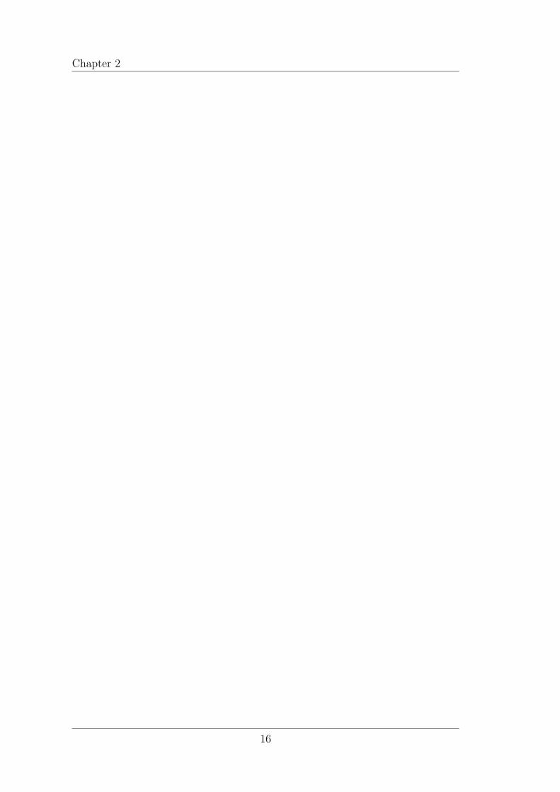
Numerical calculations for different ply lamination schemes and differ-ent boundary conditions were also held. For lamination scheme the laminationscheme 0/90 and 0/90/0 were studied.The variation of vibration with boundaryconditions of SS, SC, CC, FF, FS and FC (S stands for simply supported C forclamp and F for free end) were evaluated for levy type solution. The results werecompared with the results given by Khdeir.

These calculations were carried out for ESL theory of 1,2,3 and 4th orderand LW theory of 1,2,3 and 4th order. The result provided in this section is forESL4 and the remaining results are provided in the appendix.

The calculations were carried out for 8 different cases and the case of ESL3theory is presented in this section for comparison with Khdeir’s results.

The mean percentage difference between Khdeir’s result and ESL4 resultsin 1.69 percent with a standard deviation of 3.42. This analysis is carried outwith other higher order theories and the results are summarized in the followingtable: The above data analysis is based on all the data provided in the appendix.The above table shows that ESL3 results are the closest to Khdeirs results whichis near to the truth as Khdeir’s results were based on Reddy and Liu’s Kinematicsand that model is an extension of ESLZ1 [6]. The above table shows how thiscarrera’s approach can be used to compare the results from different theories.

28

Numerical Results

MODE 1 2 3 4 5 6 7 8SSSS 6.080 13.917 19.482 25.918 27.551 40.774 43.562 46.574Hashemi[9] 6.091 13.894 19.482 25.799 27.554 40.474 43.566 46.654Percentage error 0.174 0.168 0.001 0.462 0.010 0.740 0.008 0.172SCSC 8.400 18.150 19.482 31.032 34.401 36.716 45.988 52.069Hashemi[9] 8.370 18.016 19.508 30.721 34.345 36.704 45.413 52.016Percentage error 0.358 0.745 0.134 1.013 0.163 0.031 1.267 0.102SFSF 2.874 4.628 10.421 11.053 12.965 14.825 18.915 20.170Hashemi[9] 2.887 4.637 10.425 11.051 12.955 14.837 18.885 19.527Percentage error 0.447 0.185 0.041 0.022 0.080 0.080 0.160 3.291

Table 4.6: Higher Mode for Isotropic Spherical Shell Comparison with Hashemi’sResults using ESL4

Lamination Type of shell R/a SS SC CC FF FS FC0/90 Spherical 5 9.279 11.093 14.237 5.790 6.112 6.526

20 8.974 10.748 12.902 5.788 6.118 6.565Cylinderical 5 9.087 10.937 14.220 5.879 6.207 6.684

20 8.974 10.746 12.907 5.804 6.135 6.5870/90/0 Spherical 5 11.974 13.921 17.313 3.887 4.396 6.091

20 11.770 13.685 15.810 3.798 4.330 6.073Cylinderical 5 11.768 13.752 17.268 3.912 4.420 6.187

20 11.757 13.674 15.807 3.799 4.332 6.077

Table 4.7: ESL3 Calculation for Different Conditions


20 9 10.85 13.16 5.8 6.15 6.59Cylinderical 5 9.02 10.87 13.12 5.7 5.1 6.6

20 8.97 10.82 12.07 5.8 6.14 6.590/90/0 Spherical 5 12.06 14.1 17.57 3.9 4.41 6.11

20 11.81 13.84 16.1 3.8 4.33 6.09Cylinderical 5 11.85 13.87 16.03 3.78 4.31 6.12

20 11.79 13.83 16 3.79 4.32 6.09

Table 4.8: Solution from Khdeir[5]

29

Chapter 4

Theory Mean Percentage Error Standard DeviationESL1 4.358 4.653ESL2 3.627 4.739ESL3 1.663 3.485ESL4 1.694 3.418LW1 2.066 3.568LW2 2.212 3.502LW3 2.356 3.293LW4 2.356 3.292

Table 4.9: Percentage Error of Different Theories

It is important to note that 4.6 in not capable of showing the trendof improvement in results with an increase in the order of the theory. As thepercentage errors and standard deviations are calculated form different theoryaltogether. .

30

Conclusion

The analysis in the previous section and the data provided in the appendixshow that carrera’s approach can be applied to shell problem to find Exact freeVibration Solutions of Shells accurately. As the results match with the resultprovided by previous theories. Moreover a study of comaprison of accuracy orchange in result with changing order of the theory or the theory itself can becarried out as shown in the previous section.

In short carrera’s approach provides us with an excellent tool to performoptimization of solution accuracy and computation time and the model providedin the documents provides accurate Exact free Vibration Solutions of CompositeShells. As a recommendation for future work a study can be carried out usingfinite element tools to establish the accuracy of the given model as compared toa 3 dimensional element.

31

Bibliography

[1] A. E. H. Love. On the small free vibrations and deformations of elastic shells.Philosophical Transactions of the Royal Society of London. A Vol. 179, pp.491-546, 1888.

[2] Mindlin. Influence of rotatory inertia and shear on flexural motions ofisotropic, elastic plates. ASME Journal of Applied Mechanics, Vol. 18 pg.31–38., 1951.

[3] E. Carrera,Theories and finite elements for multilayered, anisotropic, composite platesand shells Archives of Computational Methods in Engineering,9 pg. 87-140,2002.

[4] L. Dozio,Exact vibration solutions for cross-ply laminated plates with two opposite edgessimply supported using refined theories of variable order Journal of Sound andVibration, Volume 333, Issue 8, pg 2347–2359, 14 April 2014.

[5] A. A. Khdeir and J. N. Reddy,Influence of edge conditions on the modal characteristics of cross-ply laminatedshells Computers and Structures 34(6) pg 817-826,1990.

[6] J. N. Reddy and C. F. Liu,A higher order shear deformation theory of laminated elastic shells Interna-tional Journal Engineering Sciences 23 pg 319-330,1985.

[7] S. BrishettoAn exact 3D solution for free vibrations of multilayered cross-ply compositeand sandwich plates and shells International Journal of Applied MechanicsVol. 6 Article Id 1450076 pgs 42, 2014.

[8] S. BrishettoThree-Dimensional Exact Free Vibration Analysis of Spherical,Cylindrical,and Flat One-Layered Panels Shock and Vibration Article ID 479738, 29 pg,2014

33

[9] Sh. H. Hashemi , M. FadaeeOn the free vibration of moderately thick spherical shell panel.A new exactclosed-form procedure Journal of Sound and Vibration 330, pg 4352–4367,2011.

34

Appendix A

Appendix


20 9.123 10.949 13.182 5.863 6.193 6.640Cylinderical 5 9.229 11.130 14.468 5.952 6.279 6.754

20 9.123 10.948 13.185 5.877 6.210 6.6600/90/0 Spherical 5 12.785 15.240 18.955 3.963 4.468 6.291

20 12.605 15.043 17.588 3.876 4.405 6.279Cylinderical 5 12.595 15.090 18.923 3.990 4.491 6.385

20 12.593 15.034 17.585 3.879 4.407 6.284

Table A.1: ESL1 Calculation for Different Conditions for Cross Ply LaminatedShells

35

Appendix


20 9.018 10.834 13.052 5.813 6.145 6.595Cylinderical 5 9.132 11.023 14.354 5.904 6.232 6.712

20 9.018 10.834 13.059 5.827 6.162 6.6160/90/0 Spherical 5 12.718 15.188 18.920 3.901 4.413 6.255

20 12.535 14.990 17.549 3.813 4.349 6.241Cylinderical 5 12.526 15.037 18.885 3.927 4.437 6.349

20 12.524 14.980 17.548 3.815 4.351 6.248



20 8.966 10.723 12.857 5.776 6.109 6.555Cylinderical 5 9.079 10.913 14.176 5.866 6.196 6.674

20 8.966 10.723 12.862 5.791 6.126 6.5770/90/0 Spherical 5 11.974 13.920 17.309 3.885 4.396 6.090

20 11.770 13.682 15.805 3.798 4.330 6.071Cylinderical 5 11.768 13.751 17.265 3.912 4.418 6.185

20 11.757 13.673 15.802 3.799 4.332 6.077



20 9.046 10.854 13.063 5.824 6.157 6.605Cylinderical 5 9.140 11.021 14.332 5.904 6.234 6.709

20 9.041 10.849 13.063 5.834 6.168 6.6210/90/0 Spherical 5 11.802 13.701 17.084 3.899 4.409 6.063

20 11.595 13.459 15.565 3.812 4.343 6.043Cylinderical 5 11.595 13.530 17.037 3.924 4.430 6.155

20 11.580 13.448 15.562 3.813 4.345 6.049

Table A.4: LW1 Calculation for Different Conditions for Cross Ply LaminatedShells

36

Appendix


20 8.990 10.777 12.955 5.802 6.132 6.579Cylinderical 5 9.084 10.943 14.235 5.882 6.209 6.684

20 8.985 10.773 12.955 5.812 6.143 6.5950/90/0 Spherical 5 11.690 13.538 16.896 3.887 4.395 6.030

20 11.479 13.293 15.362 3.799 4.330 6.010Cylinderical 5 11.480 13.366 16.849 3.912 4.416 6.124

20 11.465 13.282 15.357 3.801 4.330 6.016



20 8.943 10.677 12.777 5.768 6.099 6.543Cylinderical 5 9.037 10.845 14.074 5.849 6.177 6.649

20 8.938 10.673 12.777 5.777 6.110 6.5600/90/0 Spherical 5 11.684 13.507 16.840 3.879 4.387 6.023

20 11.471 13.260 15.296 3.791 4.323 6.002Cylinderical 5 11.474 13.335 16.793 3.905 4.410 6.116

20 11.459 13.249 15.291 3.793 4.324 6.009



20 8.943 10.677 12.776 5.768 6.099 6.543Cylinderical 5 9.037 10.845 14.073 5.849 6.177 6.649

20 8.938 10.671 12.776 5.777 6.110 6.5600/90/0 Spherical 5 11.684 13.507 16.840 3.879 4.387 6.023

20 11.471 13.259 15.295 3.791 4.323 6.002Cylinderical 5 11.474 13.334 16.791 3.905 4.410 6.116

20 11.459 13.248 15.291 3.793 4.324 6.009


37

Appendix

38

Exact free Vibration Solutions of Laminated Composite ... · Exact free Vibration Solutions of...

Documents

Transcript of Exact free Vibration Solutions of Laminated Composite ... · Exact free Vibration Solutions of...