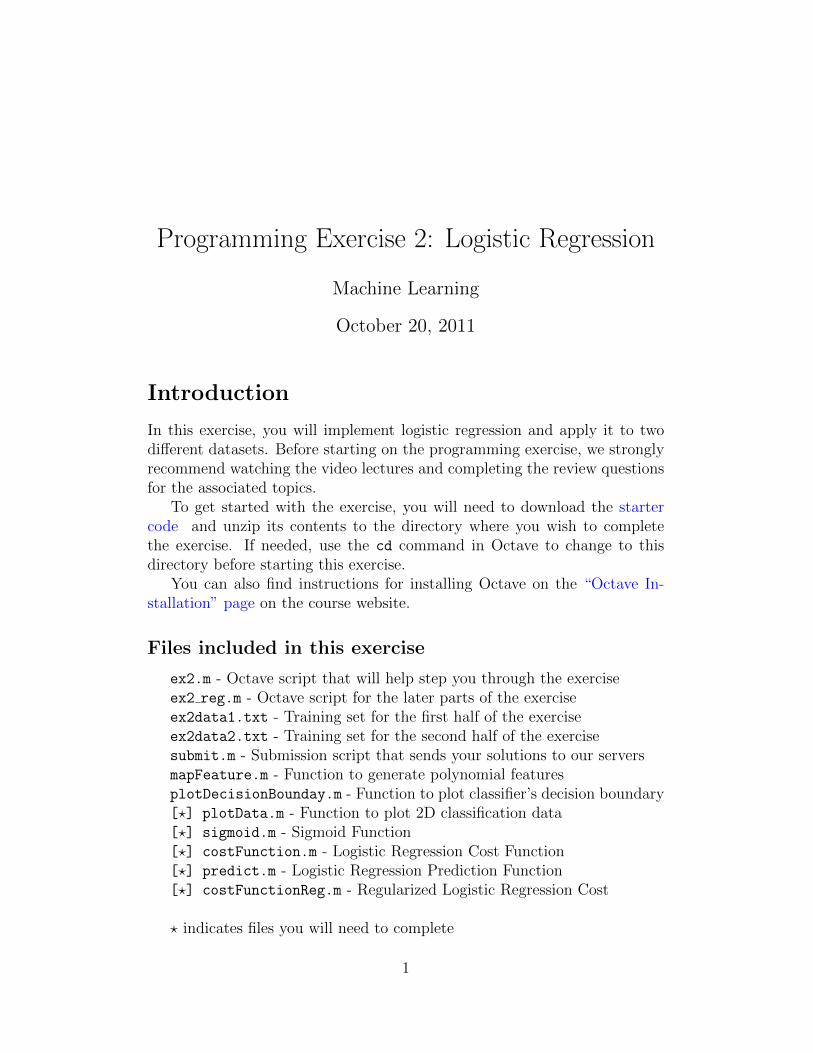
Programming Exercise 2: Logistic Regression

Machine Learning

October 20, 2011

Introduction

In this exercise, you will implement logistic regression and apply it to twodifferent datasets. Before starting on the programming exercise, we stronglyrecommend watching the video lectures and completing the review questionsfor the associated topics.

To get started with the exercise, you will need to download the startercode and unzip its contents to the directory where you wish to completethe exercise. If needed, use the cd command in Octave to change to thisdirectory before starting this exercise.

You can also find instructions for installing Octave on the “Octave In-stallation” page on the course website.

Files included in this exercise

ex2.m - Octave script that will help step you through the exerciseex2 reg.m - Octave script for the later parts of the exerciseex2data1.txt - Training set for the first half of the exerciseex2data2.txt - Training set for the second half of the exercisesubmit.m - Submission script that sends your solutions to our serversmapFeature.m - Function to generate polynomial featuresplotDecisionBounday.m - Function to plot classifier’s decision boundary[?] plotData.m - Function to plot 2D classification data[?] sigmoid.m - Sigmoid Function[?] costFunction.m - Logistic Regression Cost Function[?] predict.m - Logistic Regression Prediction Function[?] costFunctionReg.m - Regularized Logistic Regression Cost

? indicates files you will need to complete

1

Throughout the exercise, you will be using the scripts ex2.m and ex2 reg.m.These scripts set up the dataset for the problems and make calls to functionsthat you will write. You do not need to modify either of them. You are onlyrequired to modify functions in other files, by following the instructions inthis assignment.

Where to get help

The exercises in this course use Octave,1 a high-level programming languagewell-suited for numerical computations. If you do not have Octave installed,please refer to the installation instructons at the “Octave Installation” pagehttp://www.ml-class.org/course/resources/index?page=octave-install on thecourse website.

At the Octave command line, typing help followed by a function namedisplays documentation for a built-in function. For example, help plot willbring up help information for plotting. Further documentation for Octavefunctions can be found at the Octave documentation pages.

We also strongly encourage using the online Q&A Forum to discussexercises with other students. However, do not look at any source codewritten by others or share your source code with others.

1 Logistic Regression

In this part of the exercise, you will build a logistic regression model topredict whether a student gets admitted into a university.

Suppose that you are the administrator of a university department andyou want to determine each applicant’s chance of admission based on theirresults on two exams. You have historical data from previous applicantsthat you can use as a training set for logistic regression. For each trainingexample, you have the applicant’s scores on two exams and the admissionsdecision.

Your task is to build a classification model that estimates an applicant’sprobability of admission based the scores from those two exams. This outlineand the framework code in ex2.m will guide you through the exercise.

1Octave is a free alternative to MATLAB. For the programming exercises, you are freeto use either Octave or MATLAB.

2

1.1 Visualizing the data

Before starting to implement any learning algorithm, it is always good tovisualize the data if possible. In the first part of ex2.m, the code will load thedata and display it on a 2-dimensional plot by calling the function plotData.

You will now complete the code in plotData so that it displays a figurelike Figure 1, where the axes are the two exam scores, and the positive andnegative examples are shown with different markers.

30 40 50 60 70 80 90 10030

40

50

60

70

80

90

100

Exam 1 score

Exa

m 2

sco

re

AdmittedNot admitted

Figure 1: Scatter plot of training data

To help you get more familiar with plotting, we have left plotData.m

empty so you can try to implement it yourself. However, this is an optional(ungraded) exercise. We also provide our implementation below so you cancopy it or refer to it. If you choose to copy our example, make sure you learnwhat each of its commands is doing by consulting the Octave documentation.

% Find Indices of Positive and Negative Examplespos = find(y==1); neg = find(y == 0);

% Plot Examplesplot(X(pos, 1), X(pos, 2), 'k+','LineWidth', 2, ...

'MarkerSize', 7);plot(X(neg, 1), X(neg, 2), 'ko', 'MarkerFaceColor', 'y', ...

'MarkerSize', 7);

3

1.2 Implementation

1.2.1 Warmup exercise: sigmoid function

Before you start with the actual cost function, recall that the logistic regres-sion hypothesis is defined as:

hθ(x) = g(θTx),

where function g is the sigmoid function. The sigmoid function is defined as:

g(z) =1

1 + e−z.

Your first step is to implement this function in sigmoid.m so it can becalled by the rest of your program. When you are finished, try testing a fewvalues by calling sigmoid(x) at the octave command line. For large positivevalues of x, the sigmoid should be close to 1, while for large negative values,the sigmoid should be close to 0. Evaluating sigmoid(0) should give youexactly 0.5. Your code should also work with vectors and matrices. Fora matrix, your function should perform the sigmoid function onevery element.

You can submit your solution for grading by typing submit at the Octavecommand line. The submission script will prompt you for your username andpassword and ask you which files you want to submit. You can obtain a sub-mission password from the website.

You should now submit the warm up exercise.

1.2.2 Cost function and gradient

Now you will implement the cost function and gradient for logistic regression.Complete the code in costFunction.m to return the cost and gradient.

Recall that the cost function in logistic regression is

J(θ) =1

m

m∑i=1

[−y(i) log(hθ(x

(i))) − (1 − y(i)) log(1 − hθ(x(i)))

],

and the gradient of the cost is a vector θ where the jth element (for j =0, 1, . . . , n) is defined as follows:

4

∂J(θ)

∂θj=

1

m

m∑i=1

(hθ(x(i)) − y(i))x

(i)j

Note that while this gradient looks identical to the linear regression gra-dient, the formula is actually different because linear and logistic regressionhave different definitions of hθ(x).

Once you are done, ex2.m will call your costFunction using the initialparameters of θ. You should see that the cost is about 0.693.

You should now submit the cost function and gradient for logistic re-gression. Make two submissions: one for the cost function and one for thegradient.

1.2.3 Learning parameters using fminunc

In the previous assignment, you found the optimal parameters of a linearregression model by implementing gradent descent. You wrote a cost functionand calculated its gradient, then took a gradient descent step accordingly.This time, instead of taking gradient descent steps, you will use an Octavebuilt-in function called fminunc.

Octave’s fminunc is an optimization solver that finds the minimum of anunconstrained2 function. For logistic regression, you want to optimize thecost function J(θ) with parameters θ.

Concretely, you are going to use fminunc to find the best parameters θfor the logistic regression cost function, given a fixed dataset (of X and yvalues). You will pass to fminunc the following inputs:

� The initial values of the parameters we are trying to optimize.

� A function that, when given the training set and a particular θ, computesthe logistic regression cost and gradient with respect to θ for the dataset(X, y)

In ex2.m, we already have code written to call fminunc with the correctarguments.

2Constraints in optimization often refer to constraints on the parameters, for example,constraints that bound the possible values θ can take (e.g., θ ≤ 1). Logistic regressiondoes not have such constraints since θ is allowed to take any real value.

5

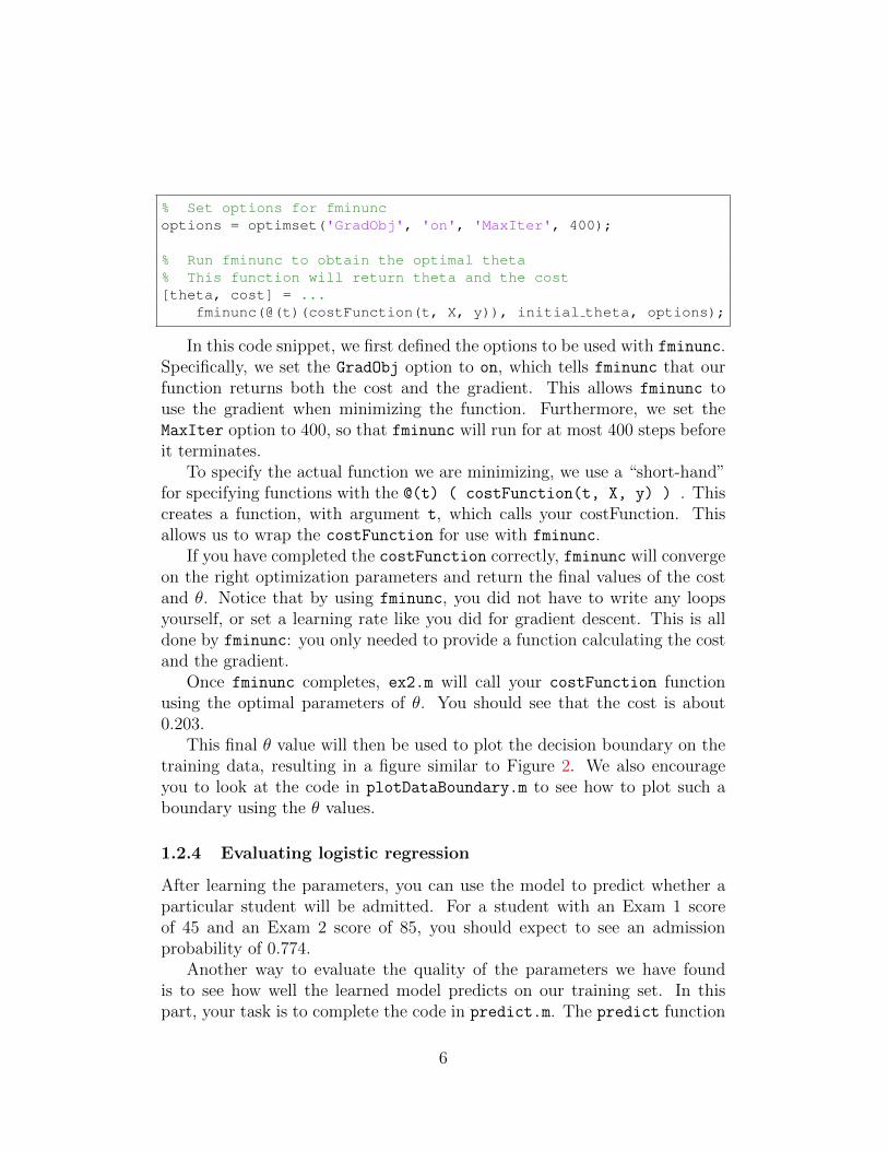
% Set options for fminuncoptions = optimset('GradObj', 'on', 'MaxIter', 400);

% Run fminunc to obtain the optimal theta% This function will return theta and the cost[theta, cost] = ...

fminunc(@(t)(costFunction(t, X, y)), initial theta, options);

In this code snippet, we first defined the options to be used with fminunc.Specifically, we set the GradObj option to on, which tells fminunc that ourfunction returns both the cost and the gradient. This allows fminunc touse the gradient when minimizing the function. Furthermore, we set theMaxIter option to 400, so that fminunc will run for at most 400 steps beforeit terminates.

To specify the actual function we are minimizing, we use a “short-hand”for specifying functions with the @(t) ( costFunction(t, X, y) ) . Thiscreates a function, with argument t, which calls your costFunction. Thisallows us to wrap the costFunction for use with fminunc.

If you have completed the costFunction correctly, fminunc will convergeon the right optimization parameters and return the final values of the costand θ. Notice that by using fminunc, you did not have to write any loopsyourself, or set a learning rate like you did for gradient descent. This is alldone by fminunc: you only needed to provide a function calculating the costand the gradient.

Once fminunc completes, ex2.m will call your costFunction functionusing the optimal parameters of θ. You should see that the cost is about0.203.

This final θ value will then be used to plot the decision boundary on thetraining data, resulting in a figure similar to Figure 2. We also encourageyou to look at the code in plotDataBoundary.m to see how to plot such aboundary using the θ values.

1.2.4 Evaluating logistic regression

After learning the parameters, you can use the model to predict whether aparticular student will be admitted. For a student with an Exam 1 scoreof 45 and an Exam 2 score of 85, you should expect to see an admissionprobability of 0.774.

Another way to evaluate the quality of the parameters we have foundis to see how well the learned model predicts on our training set. In thispart, your task is to complete the code in predict.m. The predict function

6

30 40 50 60 70 80 90 10030

40

50

60

70

80

90

100

Exam 1 score

Exa

m 2

sco

re

AdmittedNot admitted

Figure 2: Training data with decision boundary

will produce “1” or “0” predictions given a dataset and a learned parametervector θ.

After you have completed the code in predict.m, the ex2.m script willproceed to report the training accuracy of your classifier by computing thepercentage of examples it got correct.

You should now submit the prediction function for logistic regression.

2 Regularized logistic regression

In this part of the exercise, you will implement regularized logistic regressionto predict whether microchips from a fabrication plant passes quality assur-ance (QA). During QA, each microchip goes through various tests to ensureit is functioning correctly.

Suppose you are the product manager of the factory and you have thetest results for some microchips on two different tests. From these two tests,you would like to determine whether the microchips should be accepted orrejected. To help you make the decision, you have a dataset of test resultson past microchips, from which you can build a logistic regression model.

7

You will use another script, ex2 reg.m to complete this portion of theexercise.

2.1 Visualizing the data

Similar to the previous parts of this exercise, plotData is used to generate afigure like Figure 3, where the axes are the two test scores, and the positive(y = 1, accepted) and negative (y = 0, rejected) examples are shown withdifferent markers.

−1 −0.5 0 0.5 1 1.5−0.8

−0.6

−0.4

−0.2

0

0.2

0.4

0.6

0.8

1

1.2

Microchip Test 1

Mic

roch

ip T

est 2

y = 1y = 0

Figure 3: Plot of training data

Figure 3 shows that our dataset cannot be separated into positive andnegative examples by a straight-line through the plot. Therefore, a straight-forward application of logistic regression will not perform well on this datasetsince logistic regression will only be able to find a linear decision boundary.

2.2 Feature mapping

One way to fit the data better is to create more features from each datapoint. In the provided function mapFeature.m, we will map the features intoall polynomial terms of x1 and x2 up to the sixth power.

8

mapFeature(x) =

1x1x2x21x1x2x22x31...

x1x52

x62

As a result of this mapping, our vector of two features (the scores on

two QA tests) has been transformed into a 28-dimensional vector. A logisticregression classifier trained on this higher-dimension feature vector will havea more complex decision boundary and will appear nonlinear when drawn inour 2-dimensional plot.

While the feature mapping allows us to build a more expressive classifier,it also more susceptible to overfitting. In the next parts of the exercise, youwill implement regularized logistic regression to fit the data and also see foryourself how regularization can help combat the overfitting problem.

2.3 Cost function and gradient

Now you will implement code to compute the cost function and gradient forregularized logistic regression. Complete the code in costFunctionReg.m toreturn the cost and gradient.

Recall that the regularized cost function in logistic regression is

J(θ) =1

m

m∑i=1

[−y(i) log(hθ(x

(i))) − (1 − y(i)) log(1 − hθ(x(i)))

]+

λ

2m

n∑j=1

θ2j .

Note that you should not regularize the parameter θ0; thus, the finalsummation above is for j = 1 to n, not j = 0 to n. The gradient of the costfunction is a vector where the jth element is defined as follows:

∂J(θ)

∂θ0=

1

m

m∑i=1

(hθ(x(i)) − y(i))x

(i)j for j = 0

9

∂J(θ)

∂θj=

1

m

(m∑i=1

(hθ(x(i)) − y(i))x

(i)j + λθj

)for j ≥ 1

Once you are done, ex2 reg.m will call your costFunctionReg functionusing the initial value of θ (initialized to all zeros). You should see that thecost is about 0.693.

You should now submit the cost function and gradient for regularized lo-gistic regression. Make two submissions, one for the cost function and onefor the gradient.

2.3.1 Learning parameters using fminunc

Similar to the previous parts, you will use fminunc to learn the optimalparameters θ. If you have completed the cost and gradient for regularizedlogistic regression (costFunctionReg.m) correctly, you should be able to stepthrough the next part of ex2 reg.m to learn the parameters θ using fminunc.

2.4 Plotting the decision boundary

To help you visualize the model learned by this classifier, we have pro-vided the function plotDecisionBoundary.m which plots the (non-linear)decision boundary that separates the positive and negative examples. InplotDecisionBoundary.m, we plot the non-linear decision boundary by com-puting the classifier’s predictions on an evenly spaced grid and then and drewa contour plot of where the predictions change from y = 0 to y = 1.

After learning the parameters θ, the next step in ex reg.m will plot adecision boundary similar to Figure 4.

10

2.5 Optional (ungraded) exercises

In this part of the exercise, you will get to try out different regularizationparameters for the dataset to understand how regularization prevents over-fitting.

Notice the changes in the decision boundary as you vary λ. With a smallλ, you should find that the classifier gets almost every training examplecorrect, but draws a very complicated boundary, thus overfitting the data(Figure 5). This is not a good decision boundary: for example, it predictsthat a point at x = (−0.25, 1.5) is accepted (y = 1), which seems to be anincorrect decision given the training set.

With a larger λ, you should see a plot that shows an simpler decisionboundary which still separates the positives and negatives fairly well. How-ever, if λ is set to too high a value, you will not get a good fit and the decisionboundary will not follow the data so well, thus underfitting the data (Figure6).

You do not need to submit any solutions for these optional (ungraded)exercises.

−1 −0.5 0 0.5 1 1.5−0.8

−0.6

−0.4

−0.2

0

0.2

0.4

0.6

0.8

1

1.2lambda = 1

Microchip Test 1

Mic

roch

ip T

est 2

y = 1y = 0Decision boundary

Figure 4: Training data with decision boundary (λ = 1)

11

−1 −0.5 0 0.5 1 1.5−1

−0.5

0

0.5

1

1.5lambda = 0

Microchip Test 1

Mic

roch

ip T

est 2

y = 1y = 0Decision boundary

Figure 5: No regularization (Overfitting) (λ = 0)

−1 −0.5 0 0.5 1 1.5−0.8

−0.6

−0.4

−0.2

0

0.2

0.4

0.6

0.8

1

1.2lambda = 100

Microchip Test 1

Mic

roch

ip T

est 2

y = 1y = 0Decision boundary

Figure 6: Too much regularization (Underfitting) (λ = 100)

12

Submission and Grading

After completing various parts of the assignment, be sure to use the submit

function system to submit your solutions to our servers. The following is abreakdown of how each part of this exercise is scored.

Part Submitted File PointsSigmoid Function sigmoid.m 5 pointsCompute cost for logistic regression costFunction.m 30 pointsGradient for logistic regression costFunction.m 30 pointsPredict Function predict.m 5 pointsCompute cost for regularized LR costFunctionReg.m 15 pointsGradient for regularized LR costFunctionReg.m 15 pointsTotal Points 100 points

You are allowed to submit your solutions multiple times, and we willtake the highest score into consideration. To prevent rapid-fire guessing, thesystem enforces a minimum of 5 minutes between submissions.

All parts of this programming exercise are due Sunday, October 30that 23:59:59 PDT.

13