Evolutionary Growth Theory
50
Evolutionary Growth Theory J. Stan Metcalfe* and John Foster**, School of Economics Discussion Paper No. 388, April 2009, School of Economics, The University of Queensland. Australia. Full text available as: PDF - Requires Adobe Acrobat Reader or other PDF viewer ABSTRACT: We begin by outlining competing stylised facts about economic growth and then set out the relations between structural change and aggregate productivity growth contingent on the evolution of the pattern of demand. We then introduce the concept of an industry level technical progress function and show how rates of technical progress are mutually determined as a consequence of increasing returns and the changing distribution of demand. We next sketch a macroeconomic closure of the evolutionary process, expressed in terms of the mutual determination of rates of capital accumulation and rates of productivity growth. In the final section we elaborate upon the restless nature of innovation-based economic growth and the conditions under which Nicholas Kaldor’s stylised facts are compatible with the Clark-Kuznets stylised facts. We may summarise our perspective quite sharply. What distinguishes modern capitalism is not only its order imposing properties that lead to the self organisation of the economy, but also the self transforming properties that create wealth from knowledge and, in so doing, induce the further development of useful knowledge. The manner in which self-organisation and self- transformation interact in terms of adjustments to the composition of demand, as well as the structure of technology and production, is at the core of this essay EPrint Type: Departmental Technical Report Keywords: Economic growth, economic evolution, endogenous growth theory, Subjects: ID Code: JEL Classification: O33, O41, O43 Deposited By: J. Stan Metcalfe (*corresponding author) Professor Emeritus, University of Manchester. Visiting Professor University of Queensland and Curtin University of Technology, Western Australia. Visiting Fellow Centre for Business Research, Cambridge University. [email protected] John Foster** University of Queensland School of Economics Brisbane, QLD 4072 ph: + 61 7 3365 fax: +61 7 3365 7299 [email protected]
Transcript of Evolutionary Growth Theory
Evolutionary Growth Theory
J. Stan Metcalfe* and John Foster**, School of Economics Discussion Paper No. 388, April 2009, School of Economics, The University of Queensland. Australia.
Full text available as: PDF- Requires Adobe Acrobat Reader or other PDF viewer
ABSTRACT:
We begin by outlining competing stylised facts about economic growth and then set out the relations between
structural change and aggregate productivity growth contingent on the evolution of the pattern of demand. We
then introduce the concept of an industry level technical progress function and show how rates of technical
progress are mutually determined as a consequence of increasing returns and the changing distribution of demand.
We next sketch a macroeconomic closure of the evolutionary process, expressed in terms of the mutual
determination of rates of capital accumulation and rates of productivity growth. In the final section we elaborate
upon the restless nature of innovation-based economic growth and the conditions under which Nicholas Kaldor’s
stylised facts are compatible with the Clark-Kuznets stylised facts. We may summarise our perspective quite
sharply. What distinguishes modern capitalism is not only its order imposing properties that lead to the self
organisation of the economy, but also the self transforming properties that create wealth from knowledge and, in so
doing, induce the further development of useful knowledge. The manner in which self-organisation and self-
transformation interact in terms of adjustments to the composition of demand, as well as the structure of technology
and production, is at the core of this essay
EPrint Type: Departmental Technical Report
Keywords: Economic growth, economic evolution, endogenous growth theory,
Subjects:
ID Code: JEL Classification: O33, O41, O43
Deposited By:
J. Stan Metcalfe (*corresponding author) Professor Emeritus, University of Manchester. Visiting Professor University of Queensland and Curtin University of Technology, Western Australia. Visiting Fellow Centre for Business Research, Cambridge University. [email protected]
John Foster** University of Queensland School of Economics Brisbane, QLD 4072 ph: + 61 7 3365 fax: +61 7 3365 7299 [email protected]

EVOLUTIONARY GROWTH THEORY
BY
J. STAN METCALFE* AND JOHN FOSTER**
To appear in Mark Setterfield(ed)
Handbook of Alternative Theories of Economic Growth
Edward Elgar, Cheltenham.
Final version, 28th March, 2009
*Professor Emeritus, University of Manchester. Visiting Professor University of Queensland,
and Curtin University of Technology, Western Australia. Visiting Fellow, Centre for Business
Research, Cambridge University
**Professor of Economics University of Queensland. Visiting Fellow Centre for Business
Research, Cambridge University
Correspondence to stan.metcalfe @manchester.ac.uk. and [email protected]
1

“Our general conclusion must be that in the field of economic progress the notion of tendency
towards equilibrium is definitely inapplicable to particular elements of growth and with reference
to progress as a unitary process or system of interconnected changes is of such limited and partial
application as to be misleading rather than useful.” (Knight, F.H., 1935(1997), p.176)
I. Introduction
An evolutionary theory of economic growth is naturally designed to answer the all important
question “How is wealth created from knowledge?” No serious economist doubts that the
growth of per capita income and welfare is a consequence of the growth of understanding about
the human built and natural worlds but how useful knowledge is created and translated into
economic development is a matter of great complexity. At the heart of this problem is the need
for a disaggregated framework of understanding that explains much more than the rate of growth
of aggregate economic activity and the evolution of broad macroeconomic ratios. Of course,
many different theoretical frames can be consistent with the same broad aggregate facts but they
must also be consistent with many more disaggregated facts about the way a capitalist economy
develops, particularly those facts that are ultimately traceable to the role of enterprise and
creative thought in economic growth.1 Inventive creativity is part of this process, as is its
relationship to the development of formal, general scientific and technological knowledge. But
invention alone is insufficient; it must be translated into innovation, which depends greatly on
specific knowledge of time and place and conjectures of market opportunity, quite different
dimensions of knowing. Moreover, if innovations are to have significant growth effects, the
allocation of resources and patterns of demand must adapt to the possibilities opened up by new
methods and new goods and services. Market processes loom large in this scheme but so do
other instituted systems, such as the science and technology system or the education system2.
The interplay between these different forms of organisation leads to a two way interaction
between economic growth and the growth of knowledge that fully deserves to be labelled an
1 See for example Nelson and Winter (1974) where an evolutionary model of innovation is used to replicate the aggregate behaviour of a Solow-type, neoclassical growth model. The two theoretical worlds are poles apart, yet they are consistent with the same aggregate facts. 2 For a powerful exposition of knowledge related factors in economic growth, together with the importance of distinguishing different kinds of knowledge, and an understanding of the instituted context in which useful knowledge is developed and applied, see Mokyr (2002)
2

endogenous growth theory. It is the nature of the two way interaction that is the primary focus of
this paper. It is certainly not a comprehensive treatment of evolutionary growth theory but rather
an exposition of some of the links between technical progress and structural change in an
evolving economy. The foundations are Schumpeterian, and there are strong elements of
Marshall too. We build on these foundations in a way which renders compatible the diverse
circumstances of innovation and investment with aggregate patterns of economic change3. How
innovations in firms and markets “add up” to constitute industry and whole economy level
adaptations is the evolutionary problem that we are addressing.
There are three themes to this essay that follow from its evolutionary perspective. The first is
that capitalist economies grow as they develop, so that growth cannot be treated meaningfully by
a concept of uniform expansion in which all the components of an economy expand at the same
proportionate rate. Balanced growth is a chimera, it is the heterogeneity of growth rates within
the economy that needs to be explained, and differential rates of growth lead us directly to
structural change and development. It follows that an aggregate rate of growth or an aggregate
ratio has no more substance than the individual components from which it is constructed by the
observer. Indeed, even in a multi sector economy, there may be no activity which grows at the
aggregate, average rate . Consequently, the evolutionary modes of explanation used below are
essentially statistical in nature and relate to changes in population ensembles. Secondly, as the
epigraph to this essay indicates, growth is not an equilibrium process and cannot be if it is
knowledge based, for what sense is there in the idea that the growth of knowledge is an
equilibrium process?4. Yet the possibility of evolution depends on order and on the organising
processes that generate coherent structures of economic activity, whether in firms, in markets or
in other organisational forms that sit within the wider set of evolved and instituted rules of the
game (Abramovitz, 1989, Nelson, 2005). Thus there is a paradox at the centre of capitalism: the
presence of order depends on stabilizing forces that give coherence and durability to patterns of
organisation but the development of the system requires that the prevailing order is open to
invasion by economic novelty, and to this degree it is marked by instability5. It is the inherent
openness of the market system to the challenge contained in novel economic conjectures, its 3 Schumpeter (1912 and (1928) are the key texts here, and Marshall (1919) is at least as significant as Marshall (1920). 4 For complementary approaches to out of equilibrium growth theory, see Amendola and Gaffard, (1988, 1998), and Silverberg and Verspagen, (1998). 5 A stationary state is in this sense a closed economic system, a system without history as Schumpeter pointed out.
3

capacity to stimulate and resolve disagreement about better ways to allocate resources and meet
changing needs, which gives innovation and the entrepreneur such a powerful role to play in
evolutionary growth theory. This is Schumpeter’s argument but it was surely also Marshall’s
point when he identified knowledge and organisation as “our most powerful engine of
production” (1920, p.138). Thirdly, like Nelson and Winter (1982), we believe that aggregate
explanations of economic growth should be compatible with the vast diversity of micro level,
historical evidence concerning the events and processes that equate to the notions of ‘innovation’
and ‘enterprise’. Technical progress has measurable aggregate effects but it is not generated by
any aggregate process. Thus, any respectable evolutionary explanation of growth should connect
to the rich literatures which study innovation and its management, the history of technology and
business organisation, and the developing capabilities of firms and other institutions that jointly
influence the growth and application of knowledge. These literatures are natural complements to
an evolutionary theory of economic growth; they frame our understanding of the processes
generating and limiting innovation, and they provide countless empirical examples to shape our
thinking on the knowledge-growth connection.
Several formal consequences follow that differentiate an evolutionary account from modern
equilibrium growth theory, endogenous or otherwise. First, we make no appeal to the
representative agent, or more accurately described “the uniform agent”. What is statistically
representative cannot be chosen on a priori grounds. Rather, representative action is an
emergent, developing consequence of the economic process, and no evolutionary theory can
operate by eliminating diversity in economic behaviour. Indeed, our whole scheme generates
growth because of non representative behaviour. Secondly, while our economy is competitive,
we do not mean by this a state of perfect competition but rather a process of competition within
and between industries, the grand themes of Marshallian flux and Schumpeterian enterprise. The
importance of competition is not to be understood narrowly, in terms of optimal resource
allocation but, broadly, in terms of the connection between rivalry, technical progress and the
widespread diffusion of gains in real income through reductions in the prices of goods and
services. Finally, we make no sharp separation between factor substitution within a given
technique and changes in technique, for the two phenomena are inseparable. All change in
methods requires some new understanding that is only obtained by investing resources in
problem solving activities. In part this is because we do not accept the neoclassical production
4
function as a frame of analysis (Bliss 1975, Harcourt, 1972), but more fundamentally it is
because we do not reason in terms of aggregate stocks of knowledge. There is no metric to
reduce knowledge and its changes to a meaningful real aggregate, and the attempt to construct
such an aggregate serves only to disguise the role of new knowledge in the process of
development. What matters is the uneven development and ever changing heterogeneity of what
is known and understood (Kurz, 2008, Steedman, 2003; Metcalfe, 2001). This does not mean
that capital accumulation is reduced to a relatively minor, passive role in the growth process, far
from it. The accumulation of capabilities through the embodiment of new understanding in the
labour force and in the stock of capital structures is a central channel of economic growth, and
we place great emphasis on investment processes as the vehicle of change (Nelson, Peck and
Kalachek, 1967). It is important to recognise that these problems are treated here at a price. It is
that we enter the argument at the level of the industry, suppressing all the lower level evolution
that is occurring between and within firms, the evolution that is the epitomy of enterprise and
innovation. The origins of economic development and growth are not to be found at the
aggregate level, even though there are high level constraints on the evolution o f firms and
industries. At most we have half an argument but none the less an interesting half that allows us
to draw together previously unrelated strands of thought in classical and evolutionary reasoning.
The remainder of this essay is structured as follows. We begin by outlining competing stylised
facts about economic growth and then set out the relations between structural change and
aggregate productivity growth contingent on the evolution of the pattern of demand. We then
introduce the concept of an industry level technical progress function, and show how rates of
technical progress are mutually determined as a consequence of increasing returns and the
changing distribution of demand. We next sketch a macroeconomic closure of the evolutionary
process, expressed in terms of the mutual determination of rates of capital accumulation and
rates of productivity growth. This takes us to the final section where we elaborate upon the
restless nature of innovation based economic growth and the conditions under which Kaldor’s
stylised facts are compatible with the Clark-Kuznets stylised facts.
We may summarise our perspective quite sharply. What distinguishes modern capitalism is not
only its order imposing properties that lead to the self organisation of the economy, but also the
self transforming properties that create wealth from knowledge and in so doing induce the further
development of useful knowledge. It is the manner in which self organisation and self
5

transformation interact in terms of adjustments to the composition of demand as well as the
structure of technology and production that is at the core of this essay6.
II. The Competing Stylised Facts of Growth and Development
We have alluded above to the fact that economic evolution arises at multiple levels throughout
an economy of which the aggregate, whole economy level is only one element in the total
picture. Indeed, prior to the Keynesian revolution n and Harrod’s formulation of aggregate
growth theory in the late 1930s, a rich empirical and theoretical literature had developed on the
problem of secular economic change, a literature that posed the problem of economic growth in
terms of a set of meso level stylised facts relating to growth rate diversity, structural change,
innovation and the development of demand in different industries. When growth theory turned
“macro,” economists largely forgot about the between and within industry detail and replaced
one set of stylised facts with a quite different set, expressed in terms of aggregate growth rates
and ratios. The two very different, and on the surface incompatible, sets of facts are those most
usually associated with Colin Clark and Simon Kuznets on the one hand and Nicholas Kaldor on
the other. The Clark-Kuznets facts relate to patterns of growth in different industries and point
to the large scale changes in economic structure that accompany economic growth7. This is
transparent in terms of the movements in the relative importance of the “high aggregates” such
as agriculture, industry and services8 but it becomes even more manifest when we consider the
economy at more disaggregated levels where, for example, there are greater differences in rates
of growth of individual industries relative to the manufacturing average, and even greater
differences in the growth rates of individual firm relative to an industry average. Consequently
there are large inter and intra sectoral shifts in shares in output, employment, and capital stocks
over time that reflect a wide dispersion of growth rates around the economy wide averages9.
These shifts are also associated with the entry of new industries and the elimination of old
industries along the lines that leading economic historians rightly emphasise (Sayers, 1950,
6 That an economic order is self transforming is not to be taken for granted but depends on wider instituted and encultured factors that overcome the conserving tendencies which reinforce the prevailing order. See Mokyr (2002) Chapter 6 for an extended discussion, and Nelson, (2005) Chapters 5&8. 7 See Colin Clark, (1944) and Kuznets (1971) for original statements of the relation between aggregate growth and large scale structural change. Saviotti and Pyka (2004) simulate industry entry and exit effects in an evolutionary growth model. 8 For some interesting commentary see Baumol et al. (1989, chapter 3). The idea that development is a process of reducing the relative importance of agriculture is a common theme among development economists. 9 See Kuznets (1971) Chapter 7 for the details, particularly table 4.
6

Landes, 1969, Mokyr, 1990, 2002). On this the historical record is absolutely clear; measured
economic growth flows from a process of structural change driven by long sequences of
innovations in technique and organisation that may usefully be summarised as distinct technical
epochs (Freeman and Louca, 2001).
However, this uneven pattern of the growth record is only part of the picture. Simon Kuznets
(1929) and Arthur Burns (1934) also identified a further regularity in the process of restless
growth, namely retardation, the persistent tendency of industry growth rates to decline over time
from the inception of the industry. Soloman Fabricant (1940, 1942) found compelling evidence
on the retardation of growth in American manufacturing output and employment over the period
1899 to 1939. Further studies, by Hoffman (1949), Stigler (1947) and Gaston (1961) also
investigated the empirical basis of the retardation thesis in different bodies of industrial data but
without any further development of the underlying theory. Taken together these authors might
be described as espousing “a moving frontier” view of economic growth and structural change,
in which, in Kuznet’s words,
‘As we observe various industries within a given national economy, we see that
the lead in development shifts from one branch to another. A rapidly developing
industry does not retain its vigorous growth forever but slackens and is overtaken
by others whose period of rapid development is beginning. Within one country
we can observe a succession of different branches of activity in the vanguard of
the country’s economic development, and within each industry we can notice a
conspicuous slackening in the rate of increase’ (Kuznets, 1929/1954, p. 254).
By contrast, Kaldor’s (1961) stylised facts refer to the rough constancy of the growth rates of
aggregate output and capital stocks together with the constancy of several key aggregate ratios,
particularly, the capital output ratio, the shares of profits and contractual incomes in GDP, and
the overall rate of profits (Maddison, 1991). To understand the relation between these very
different facts is a major challenge to our thinking about economic growth, not least because the
familiar devices of semi-stationary growth (Bliss, 1975), or proportional dynamics (Pasinetti,
1993) are no more than ways to hide from view the Clark-Kuznets facts, as if the relative
7

proportions of different activities are frozen in time10. There is neither structural change nor
retardation in these contrived macro worlds only uniform expansion or, just as readily, uniform
contraction. In approaching the analysis of economic growth in this way, we effectively rule out
any meaningful connection between the growth of knowledge and the growth of the economy.
Several recent contributions have addressed this problem of reconciliation by developing
frameworks in which rates of growth of demand and/or rates of technical progress differ sector
by sector. In many of these frameworks the rates of technical progress are treated exogenously,
and that is an unhelpful restriction, which is certain to misrepresent the relation between the
growth of knowledge and the development of the economy11
The important insight here is not that structural change and the growth of aggregate measures
occur together, for that would be quite compatible with the idea of structural change as a passive,
inessential by-product of growth. If that were all that were at stake, a macro, single sector
approach would be a plausible first step. Unfortunately, this is not so; structural change is not
only a consequence of differential growth it is a cause of that differential growth. This process is
autocatalytic, progress generates progress, structural change generates structural change, which
is what we take Schumpeter to have meant when he wrote of “development from within”, or
what Frank Knight meant when he described growth in capitalism as a “self-exciting” process.
Precisely what one might expect to occur in an economy whose long run evolution is driven by
new knowledge, by entrepreneurial conjecture and by the reallocation of resources to take
advantage of the opportunities immanent in innovation.
To term this an evolutionary process is entirely appropriate. The mutual determination of growth
rate differences within a population is a leading, if not the defining, characteristic of evolutionary
theory. Moreover, the more we disaggregate any given population into its component sub
populations the more we find evidence for differential growth over any given period, and the
10 This is not to deny that proportional dynamics has its uses as, for example, in the Von Neumann growth model. However, this method seems entirely incapable of addressing the two-way relation between the growth of knowledge and the growth of economic activity. Does any economic historian ever find proportional dynamics a useful device with which to order the record of the past? We think not. 11 See for example, Kongsamut et al (2001), Ngai and Pissarides (2004), Echevarria (1997), and Acemoglu and Guerrieri (2008). For a very good synopsis of the developing literature, and of the different kinds of stylised facts, the reader is referred to the paper by Bonatti and Felice (2008). This latter paper is more closely connected to our approach than any of the other papers refereed to above, since the authors incorporate endogenous technical progress into their two sector model by effectively assuming a Kaldor style technical progress function (as do we). They also assume non homothetic preferences, equivalent to our reliance on Engel’s Law, and differentiated income elasticities of demand, sector by sector. Nonetheless our approaches to the broad problem are very different.
8

longer that period the greater the diversity of growth experience. Thus there is a simple
evolutionist’s maxim that must always be born in mind, namely, “the more we aggregate the
more we hide the evidence for and causes and consequences of economic evolution”. The
evolutionary question is “Why do rates of growth differ across activities and over time?” not the
question “Why are they uniform and stable?”
It is because a macro perspective hides the very processes that explain the differential growth of
productivity and output that we cannot confront many of the most important stylised facts of
modern economic growth (Kuznets, 1954, 1971, 1977; Harberger, 1998). Nor can we
incorporate the role of demand in shaping growth patterns between industries; indeed it is
remarkable how the modern growth story is a predominately supply side account of the
expansion of productivity and inputs. Changes in the composition of demand are ignored and the
coordinating role of markets in the growth process is lost from view. Our approach therefore
places two processes at the heart of evolutionary growth, the endogenous generation of industry
specific rates of technical progress, and the endogenous evolution of demand as growing per
capita income is reallocated across different lines of expenditure. Let us consider each one in
turn.
At the core of any theory of endogenous growth we find some hypothesis about the origination
of innovation and its impact on methods of production. Our approach develops the notion of an
industry specific technical progress function that follows from Adam Smith’s central idea linking
technical progress to the changing division of labour within and between activities, and its
subsequent elaboration by Allyn Young (1928). Developing from roots in Smith and Marshall,
Young articulated the view that the extension of the market causes and is caused by the
exploitation of new technological opportunities. We shall suggest below that this is precisely the
insight needed to capture the link between structural change and aggregate growth. Of course,
the scope of Young’s argument was much broader than the linking of growth of market and
technical progress within a single industry. What mattered was the reciprocal dependence
between different industries in which ‘inventions’ in one sphere initiate ‘responses elsewhere in
the industrial structure which in turn have further unsettling effect’ (op. cit., p. 532). For Young,
9

for Schumpeter and for Marshall, progress is systemic and the idea of capitalism as a system in
equilibrium did not hold much appeal12.
As soon as we abandon the equi-proportional method there is immediate scope for giving
demand side forces a key role in the explanation of structural change, and for giving far more
attention to the role of demand in the connection between growth and technical change. As
Pasinetti has expressed it “... any investigation into technical progress must necessarily imply
some hypotheses ... on the evolution of consumer preferences as income increases”, while
“increases in productivity and increases in income are two facets of the same phenomenon, since
the first implies the second, and the composition of the second determines the relevance of the
first, the one cannot be considered if the other is ignored” (our emphasis, 1981, p. 69). This is
the territory marked out by Engel’s law, not only in terms of the broad aggregates in relation to
agriculture, industry and services but also in terms of income elasticities for the more narrowly
defined outputs of specific industries (Kindleberger, 1989).
The mutual interdependence between the differential growth of demand and the differential
incidence of technical progress is at the centre of our evolutionary account of growth and
development. But we are not free to propose any pattern of economic evolution independently of
the constraints implicit in the requirement that aggregate saving equals aggregate investment.
This leads to the central importance of Harrod’s insight that the aggregate rate of growth also
depends on the interaction between capital productivity and thrift. This is what our frame is
meant to capture in terms of the simultaneous evolution of the macro and the sectoral such that
the one cannot be explained independently of the other. It is a frame that, because it is both
“bottom up” and “top down,” allows us to render compatible the competing stylised facts.
III. The Population Method: Accounting for Structural Change and Economic Growth
An economy with many industries in which each industry engages in many different activities is
of a level of complexity that places a great challenge to any growth theory. Yet, if we
understand an economy to be a population of different activities, a method of analysis 12 For a excellent account of Young’s approach and its relation to the wider literature on economic development and cumulative causation see Toner (1999). The problem of cumulative causation is precisely the problem addressed here in terms of the disaggregated connections between increasing returns and the aggregate growth of per capita income.
10

immediately becomes apparent, one that is central to all evolutionary theories of a variation-cum-
selective retention kind. This is the method that we call population analysis. In it an
evolutionary population is represented by a set of differentiated entities that are acted upon by
common causal forces to transform the population, either by changing the constituent entities or
by changing their relative importance. In our case the entities are distinct industries. The
common causal forces are the reallocation of demand across the industries as per capita income
increases, the different rates of technical progress in each industry and the constraint imposed by
the equality of saving and investment in the aggregate. One of the immediate advantages of the
population method is that it can be conducted at multiple, interconnected levels so that change at
one level correlates with change at other levels. Thus we could also treat each industry as a
population of different branches of “similar but not identical” activities, and each such branch as
a further population of closely competing firms. In this way an economy becomes a population
of populations of populations. Even the firm could be analysed as a population of different
activities under unified managerial control if we wanted to conduct the argument at its most
refined level. For expositional reasons we must suppress the below industry level of
aggregation, recognising that a full account of technical progress at the level of the industry
necessarily requires an analysis of the differential innovation performance of firms and their
differential rates of growth. All we need say here is that our knowledge-based economy is co-
ordinated in the sense that that the average price within an industry is a long run normal price, set
to maintain full capacity utilisation over time. Short period deviations from full capacity
working are ignored, as seems appropriate in a treatment of sustainable growth. What we loose
is any account of the within-industry determinants of prices and profitability and thus of the
within-industry role of dynamic coordination through competition. However, intra industry
analysis is already well developed in evolutionary economic theory, whereas the aspects treated
here are not (Andersen 2004, ,Witt, 2003, Dosi, 2000, Metcalfe 1998, Nelson and Winter 1982).
One of the principal attributes of the population method is its connection with the statistical
method of analysis that is common ground in modern evolutionary theory. This is reflected in the
fact that the rate and direction of evolution in a population depends on statistical measures of the
variety that are defined over that population. In the presence of pervasive heterogeneity we use
the population moments of various industry characteristics, (means, variances, covariances and
11

so on), to understand the rate and direction of evolutionary change in that population. Here the
three principle characteristics in which the industries vary are, their prevailing levels of
productivity, their income elasticities of demand, and their technical progress functions.
Additional dimensions of differentiation are not ruled out; indeed the greater the number of
dimensions of variation the richer is the evolutionary analysis in prospect. The population
moments that play a central role in the evolutionary approach are always weighted moments,
where the weights are the appropriate measures of the relative importance of each industry in the
population. The weights capture the immediate structure of the population and change in
response to the divergent rates of growth within that population. Moreover, because the weights
are changing so are the moments that they are used to construct. The system is restless and we
do not need to assume that its motion is governed by a stable attractor to which it is converging:
which is fortunate, for the very process of movement necessarily revises the terms and conditions
for future movement.
Within the total population of industries that defines our economy we identify three classes of
structural change: there is the differential growth of the industries that continue in operation over
some time interval; there is the entry of new industries; and, there is the exit of existing
industries. Over a short interval of time the aggregate growth of the whole population is
accounted for by , where engg c −+= g is the growth rate of the ensemble of total activity,
is the growth rate of the aggregate of the continuing industries, is the proportionate increase in
output associated with newly created industries (the industry birth rate), and is the
proportionate loss of output associated with industries that disappear (the industry death rate)
cg
n
e13.
For short intervals of time these birth and death rates may be of negligible importance but over
longer intervals they may make up the bulk of the explanation of population level change.
Indeed, for sufficiently long intervals the output of continuing industries may be of negligible
importance: that is to say, the sets of industries that define the economy at any two census dates
may have few elements in common. However, any newly born industries can only increase their
relative importance if they grow more quickly than the average population, just as the industries
which have disappeared will have grown less rapidly than the economy as a whole. Entry and
exit matter qualitatively but they only matter quantitatively in terms of the subsequent and 13 See Metcalfe (2008) for a more detailed examination of the statistical nature of evolutionary population analysis.
12

antecedent rates of differential expansion. Hence we shall focus exclusively on this factor of
differential expansion and contraction, considering rates of growth defined over short intervals
and setting the net industry entry rate equal to zero
We must now be precise about the characteristics of each vertically integrated industry. Each
one consists of a group of firms supplying final output ready to be consumed or invested,
together with a group of firms supplying the produced means of production to produce the final
goods. When we speak of employment, or investment we refer to the total quantities in the
supply chain that support the current output of the final good, including investments to expand
capacity to produce the requisite intermediate goods. The technology of each vertically
integrated industry is reflected in a pattern of division of labour and specialisation which in turn
reflects the different technological and organisational knowledge bases of each component
activity. In relation to technology and organisation, the capital coefficient, ‘ ’ (the ratio of
capital stock in the whole integrate industry to the capacity output for the final good) is assumed
to be different for each industry. Moreover, all innovations are assumed to be Harrod neutral
process improvements; progress is purely labour augmenting within the entire supply chain. Let
be defined as unit labour requirements within the supply chain required to produce full
capacity output, then labour productivity for the industry, again measured in terms of capacity
output, is . Notice carefully that at levels of aggregation above the industry, the
ensemble input proportions will change in response to the different final output growth rates of
the various integrated industries. However, this is not factor substitution in the traditional sense,
for there is no smooth industry production function, it is instead factor reallocation or between-
industry adaptation and it is the reallocation or adaptation effects that play a central role in this
evolutionary growth theory
jb
ja
jj aq /1=
III a Measures of Population Structure
We need just two measures of population structure to capture the relative importance of each
vertically integrated industry- one in terms of its share of aggregate employment, , the other in je
13

terms of its share in aggregate capacity output, .jz
je
14 Once we know the population structure we
can immediately translate industry labour efficiency (and its inverse labour productivity) into
their population equivalents: reflecting the fact that each industry contributes to aggregate
productivity in proportion to its share in total employment, and to aggregate unit labour
requirements (efficiency) in proportion to its share in capacity output. It follows that average
unit labour requirements are and average labour productivity is , from
which it follows that, .
∑= iiz aza
1
ej qz= z
jje qeq ∑=
=ez qa
jj qe
Some elementary but important aspects of population accounting now follow from these
definitions. First there is a structural consistency condition
and zjj aa . (1a) =
From (1a) it follows immediately that the employment structure will differ from the output
structure as individual productivity or efficiency levels deviate from their population averages. It
also follows that the proportional rates of change in these measures are related by the
conservation conditions15
zaq ˆˆ (1b) = −e
jj zqe ˆˆˆ eq and zjjj aeaz ˆˆˆˆ +=+ (1c) =+ +j
This is the dynamic counterpart to the proposition that the employment and output share weights
for any industry are equal only when it has a level of productivity equal to the population
average. We can see immediately that proportional growth necessarily implies the absence of
14 The measure of output shares is contingent on the particular set of price weights used to construct the aggregate measure of capacity output, just as the employment shares are contingent on the prices of different kinds of labour within the employment aggregate. The shares in final output are different from the shares in value added industry by industry. The two differ by the product of the economy wide ratio of intermediate to final output and the fraction of the value of total intermediate output used by an industry. 15 We use a carat over a variable to indicate its logarithmic rate of change, and a dot above a variable to indicate its differential rate of change.
14

structural change, structure is frozen, and from this it follows that each industry must have the
same rate of productivity and efficiency increase, a requirement that is not conformable to the
facts. One immediate corollary is that if, say, we hold the employment share constant in some
industry then, in general, the corresponding output share cannot be constant. The converse is also
true. Notice also, that the wider the spread of productivity levels in the population the greater the
difference between output shares and employment shares.16
These accounting relations are no more than bookkeeping devices but they provide the necessary
connections between investment, technical progress and the changing pattern of demand as we
can now establish. Investment is important in three complementary ways: as the means to
expand productive capacity; as a generator of aggregate demand; and as the carrier of new
knowledge and stimulant to productivity growth. This is the sense in which we have a long run
growth theory; it is a theory dependent on the determinants and consequences of investment
activity. However, by the long run we do not mean some date far into the hypothetical future
when the economy has converged to a steady expansion path but rather the immediate present
when long run forces of investment and technical progress are active. As in Marshall’s analysis,
different causal forces are working at every moment but with different velocities, and the
different velocities are the generators of structural change and evolution.
III b. Demand and Aggregate Productivity Growth
Just as the production side of the economy can be analysed as a population of industries, so the
demand side can be analysed as a population of final consumers, such that the final demand for
the output of any one industry depends on the number of consumers it has and the rate at which
they consume. We assume that the driving causal processes behind changes in the pattern of
demand are employment growth in relation to the number of consumers, and the growth of per
capita income (the consequence of the growth of aggregate productivity) in relation to their rates
of consumption. In this scheme, productivity growth reduces prices relative to money incomes
and the consequent increase in real income generates a redistribution of expenditure over the
16 Carlin et al (2001) point out that the 90th decile of the UK manufacturing productivity distribution is almost five times more productive in labour productivity terms than the 10th decile.
15

different industries, the Engel law effects that we referred to above. That the rates of growth of
demand differ across industries, differences that would become more marked the lower the level
at which we construct our industry aggregates, is not only one of the most important empirical
regularities in economics, it is the reason why proportional growth models cannot capture the
process of economic growth in a substantial way17.
Let the per capita income elasticities for each industry, jψ , be defined as the ratio of the growth
in per capita demand for the output of each industry to the growth rate of aggregate per capita
income, thus
ngng
z
jj −
−=ψ (2)
Where, is the rate of growth of total employment, and n jjz gzg ∑= is the rate of growth of
aggregate output18. These elasticities provide us with the basis for a selection process across the
set of industries since they give rise to different growth rates of demand and output. The
simplification, that employment growth is neutral in its demand composition effects, is precisely
that, a convenient simplification. What matters is that per capita income growth and population
growth have differential demand effects and this is what we have captured in (2) and in its
consequences below. Of course, in emphasising the role of income elasticities in the inter- 17 That we ignore pure substitution effects but not the income effects of price changes is simply a consequence of not delving below the level of the industry where prices are determined. See footnote37 below, for further comment on the role of pure substitution effects. 18 If we distinguish two final uses for each good, in consumption and in investment, we can further decompose these total elasticities as follows ( ) Ijicjjjj sicsz ψψψ +−= 1 where is the aggregate saving ratio, is the fraction of the industry’s output absorbed in consumption, and is
the corresponding fraction absorbed in investment (
s jc ji1=+ jj ic ). Thus cjψ is the per capita consumption
elasticity, and jIψ is the per capita investment elasticity for industry j. Summing across the industries yields the relation ( )∑ +−=== Icjjz ssz ψψψψ 11 A constant saving ratio, as assumed below, implies a unitary income elasticity of demand for wealth. See Laitner (2000) for an analysis of non-unitary income elasticities for assets and the growth process.
16
industry selection process, we should not be deluded into thinking that we have said anything
terribly profound. The elasticities are averages taken across the population of consumers,
contingent on the distribution of tastes, on the distribution of income (both personal and
functional) and on the particular prevailing pattern of expenditure across very different
commodities. What we need is some empirical and conceptual understanding of the
determinants of income elasticities in general, their relation to the distribution of income, and
how they change in relation to innovation and the entry of new industries. This we do not yet
have, nor do we need it for immediate purposes19.
From (2) we can write the rate of output growth of each industry as
ejj qng ˆψ+= (3)
where ee qdtdq logˆ = is the, yet to be constructed, aggregate rate of productivity increase. The
immediate consequence of this formulation is that the rate of growth of each industry cannot be
determined before we have determined the rates of growth of employment and productivity
across the entire population ensemble. Thus, the pattern of industry growth rates that emerges is
simultaneously determined with the aggregate rate of growth of employment and of productivity.
The pattern of structural change in terms of output follows immediately from (3) since
( ) ( ) ezjjzjjj qzggzz ˆψψ −=−=& (4a)
An industry gains or loses relative importance in the ensemble of total (capacity) output as its
income elasticity is greater or less than the population average income elasticity, which, of
course, necessarily takes the numerical value of one. However, the proximate driver of the
changes in structure is the growth of average per capita income; without technical progress the
output structure of the population and its employment structure are frozen in time.
19 See Bianchi (1998) and Saviotti (2001) for a very useful discussion of innovation and consumer behaviour relevant to these questions.
17

Relation (4a) is our first example of the use of the replicator dynamic principle, in which the
changing economic weight of an industry depends on how its characteristics compare to the
population average of those characteristics.20 The importance of the replicator dynamic is that
provides a way of analysing economic change that is independent of any assumption of the
existence of a long run attractor towards which the economy is converging. In an open,
knowledge driven economy there cannot reasonably be expected to be any such stable attractor,
for the very movement towards it would create new knowledge, new entrepreneurial conjectures
and thus change the foundations of that attractor. Replicator dynamics sidesteps these inherent
difficulties by making the relevant rates of change dependent on the distributions of industry
characteristics around their current population averages, while simultaneously providing an
explanation of how those averages are changing. We have already pointed out that evolutionary
analysis is inherently statistical in the sense that it relates different statistical moments within a
causal structure, and an immediate illustration of this principle can be found in the relation
between the variance of the industry growth rates and the variance in the income elasticities of
demand, which, making use of (4a) is given by
( ) ( ) ( )ψzezzii VqgVggz 22 ˆ==−∑ (4b)
where ( )jzV ψ is the capacity weighted variance in the income elasticities of demand. The
greater the rate of productivity growth the greater is the variance in the industry growth rates for
a given variance in the income elasticities, and the greater is the resultant turbulence in the
capacity shares.
There is an implication of the replicator principle which is worth drawing out at this point. It is
that the income elasticities of demand cannot all be constant in a progressive economy, unless,
trivially, they are all equal to one, the necessary condition for proportional growth. This is a
deduction that is already implicit in Engel’s law in which the elasticities decline with increases in
20 See Montobbio, 2002 for an exposition of the replicator principle in the context of industry dynamics.
18

per capita income. It follows because the population average elasticity zψ =1 is a constant even
though the structure of demand is evolving according to (3). Consequently,
∑ ∑ =+ 0jjjj zz ψψ &&
and from (4b) this becomes
( ) ( )∑ ∑ −=−−= jzejzjjejj Vqzqz ψψψψψ ˆˆ&
It follows that 0=∑ jjz ψ& if, and only if, productivity growth is zero or if all income elasticities
are the same (unity in value). The former assumption rules out technical progress, the latter rules
out structural change. Hence we are left with the requirement that in a progressive economy
. On average the income elasticities must decline as productivity grows, although
this constraint is quite consistent with some of them increasing. This result is an example of
what evolutionists call Fisher’s Principle, after the eminent biologist who first formulated some
of the statistical rules of population dynamics.
∑ < 0jjz ψ&
21 It will recur in many different guises below.
III c. Aggregate Productivity Growth
We can now explore the implications for the relation between productivity growth in the
individual industries and productivity growth for the entire economy. This is not as
straightforward as it might seem, because the movement in the ensemble averages for
productivity or efficiency is composed of two components, technical progress in each industry
and structural change. Thus, for example, since jje qeq ∑= , it follows from (1a) that the
aggregate rate of productivity growth is given by
21 See Andersen, (2004), Foster, (2000) , Knudsen, (2004) and Metcalfe (2008) for further analysis and critical discussion of Fisher’s Principle. Aldrich, et al., (2008) provide a detailed, general discussion of evolutionary variation-cum-selection dynamics.
19

jjjje ezqzq ˆˆˆ ∑+∑= (5a)
With a similar expression applying to the change in average efficiency, thus
∑ ∑+= jjjjz zeaea ˆˆˆ (5b)
In relations (5a) and (5b) the aggregate rate of change is the sum of the average technical
progress effect and the average structural change effect; two terms that are often called the
“within industry effect” and the “between industry effect” in modern productivity accounting
exercises22. However, our hypothesis on demand dynamics allows us to elaborate further the
structural change effect and to write as proportional to the weighted sum of the industry
productivity growth rates.
eq
jn23 Since is the rate of growth of employment in industry j
and , it follows that njjj qng ˆ+= jejj qq ˆˆn −=− ψ . If we weight this last expression by the
employment shares and sum across the population of industries we find that je
( ) ( ) 0ˆˆ =∑−∑=−∑ jjejjjj qeqenne ψ
since by definition. Thus, our weighting scheme is provided by nne jj =∑
jjjj
e qee
q ˆ1ˆ ∑∑
=ψ
(6a)
Unless, 1=∑ jje ψ , these weights do not sum to unity. Indeed, it follows immediately that the
employment weighted income elasticity is given by
( )
∑ −==e
jjeejj q
qCe
,1
ψψψ (6b)
22 There is an extensive literature on this topic. See Bartlesman and Doms, (2000), Disney et al, (2003), Baldwin and Gu, (2005), and for an evolutionary perspective, Nelson, (1989) and Metcalfe and Ramlogan (2006) 23 See Cornwall and Cornwall (2002) for a closely related derivation.
20

Where, ( )jje qC ,ψ is the ‘ e ’ weighted covariance between productivity levels and income
elasticities across the population of industries. Thus, the employment-weighted average of the
income elasticities coincides with the output weighted average only if this covariance is zero.
By an analogous argument, the rate of decline in unit labour requirements is given by
e
jjz
aea
ψ∑=
ˆˆ (7a)
And here we can express the employment weighted income elasticity as
( )z
jjzjj a
aCe
,1
ψψ +=∑ (7b)
where ( )jjz aC ,ψ is the corresponding ‘ ’-weighted covariance between industry income
elasticities and average unit labour requirements in each industry
z
24. The employment weighted
average income elasticity plays an important role in our analysis of aggregate growth and
structural change, a result which could not be readily anticipated.
To explore this point further, we can establish how much of the overall growth of productivity or
efficiency is due to structural change and how much is due to technical progress proper.
Consider first the decomposition of changes in . Let za aσ be defined as the proportion of the
rate of change in aggregate efficiency that is due to output structural change. Then we find from
(5b) and (7b) that ea ψσ −= 1 . It follows that the corresponding proportion of aggregate labour
efficiency change that is due to technical progress, aσ−1 , is equal to eψ . Consequently
if ( ) 0, =jjz aC ψ ,( 1=eψ ), then the contribution of structural change to average efficiency
growth will be zero even though the output structure is changing. Moreover, if this covariance is
positive, then changes in the structure of output are offsetting the effect of technical progress in
24 To derive this result, write, ( ) jjjjjjj zeze ψ = ∑ ψ + ∑ − ψ∑ and recall that , with
. The analogous result in (6b) is proved similarly. jjzj azae =
jjz aza ∑=
21
the generation of average efficiency change, because demand is shifting relatively in favour of
industries that have above average unit labour requirements.
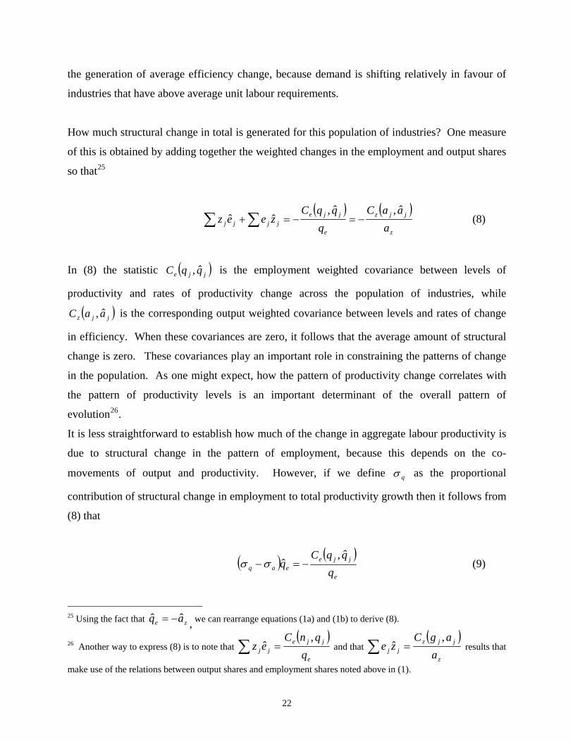
How much structural change in total is generated for this population of industries? One measure
of this is obtained by adding together the weighted changes in the employment and output shares
so that25
( ) ( )∑ ∑ −=−=+
z
jjz
e
jjejjjj a
aaCq
qqCzeez
ˆ,ˆ,ˆˆ (8)
In (8) the statistic ( )jje qqC ˆ, is the employment weighted covariance between levels of
productivity and rates of productivity change across the population of industries, while
( )jjz aaC ˆ, is the corresponding output weighted covariance between levels and rates of change
in efficiency. When these covariances are zero, it follows that the average amount of structural
change is zero. These covariances play an important role in constraining the patterns of change
in the population. As one might expect, how the pattern of productivity change correlates with
the pattern of productivity levels is an important determinant of the overall pattern of
evolution26.
It is less straightforward to establish how much of the change in aggregate labour productivity is
due to structural change in the pattern of employment, because this depends on the co-
movements of output and productivity. However, if we define qσ as the proportional
contribution of structural change in employment to total productivity growth then it follows from
) that
(8
( ) ( )e
jjeeaq q
qqCq
ˆ,ˆ −=−σσ (9)
25 Using the fact that , we can rearrange equations (1a) and (1b) to derive (8). ze aq ˆˆ −=
26 Another way to express (8) is to note that ( )
∑ =e
jjejj q
qnCez
,ˆ and that
( )∑ =
z
jjzjj a
agCze
,ˆ results that
make use of the relations between output shares and employment shares noted above in (1).
22
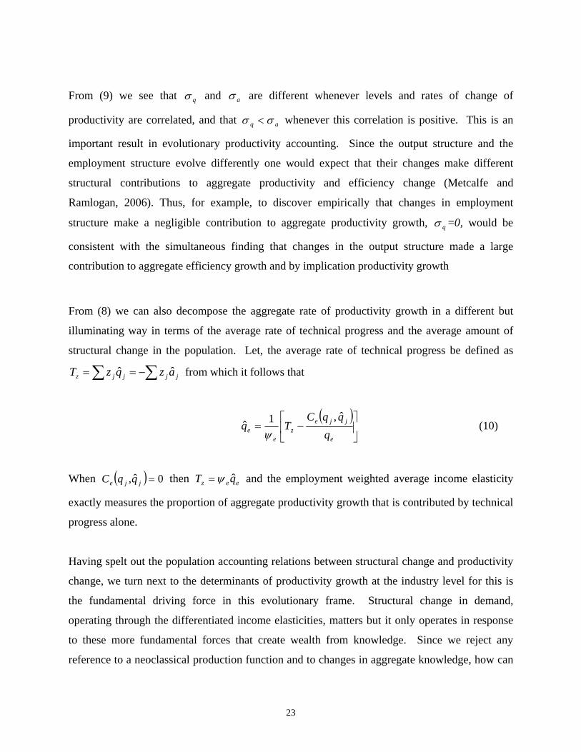
From (9) we see that qσ and aσ are different whenever levels and rates of change of
productivity are correlated, and that aq σσ < whenever this correlation is positive. This is an
important result in evolutionary productivity accounting. Since the output structure and the
employment structure evolve differently one would expect that their changes make different
structural contributions to aggregate productivity and efficiency change (Metcalfe and
Ramlogan, 2006). Thus, for example, to discover empirically that changes in employment
structure make a negligible contribution to aggregate productivity growth, qσ =0, would be
consistent with the simultaneous finding that changes in the output structure made a large
ontribution to aggregate efficiency growth and by implication productivity growth
structural change in the ge rate of technical progress be defined as
from which it follows that
c
From (8) we can also decompose the aggregate rate of productivity growth in a different but
illuminating way in terms of the average rate of technical progress and the average amount of
population. Let, the avera
∑∑ −== jjjjz azqz ˆˆT
( )⎥⎦
⎤⎢⎣
⎡−=
e
jjez
ee q
qqCTq
ˆ,1ˆψ
(10)
When ( ) 0ˆ, =jje qqC then eez qT ˆψ= and the employment weighted average income elasticity
exactly measures the proportion of aggregate productivity growth that is contributed by technical
rogress alone. p
Having spelt out the population accounting relations between structural change and productivity
change, we turn next to the determinants of productivity growth at the industry level for this is
the fundamental driving force in this evolutionary frame. Structural change in demand,
operating through the differentiated income elasticities, matters but it only operates in response
to these more fundamental forces that create wealth from knowledge. Since we reject any
reference to a neoclassical production function and to changes in aggregate knowledge, how can
23

we build an account of the self-transformation of industries and economies? Such an account
should generate the transformation process “from within”, it should connect with the sector-
specific growth of knowledge and it should emphasise the fundamental features of enterprise in
relation to investment and innovation. If we are to choose any principle that draws together
these desiderata it is that the division of labour is limited by, and in turn limits, the extent of the
market. Changes in the division of labour require changes in technology in the broad, and
extension of the market requires the growth of per capita income. No other principle would
seem to have the ability to unify the transformation of production methods and the extension of
emand to create an endogenous theory of enterprise and economic transformation.
Investment and a Technical Progress Function
d
IV
a major channel through which technical
dvances “cut into unit labour requirements” (p. 96)
In a remarkable empirical investigation into the growth of manufacturing in the USA over the
period 1899-1939, Solomon Fabricant (1942) drew attention to the fact that rapidly growing
output in an industry is usually associated with rising employment and increasing labour
productivity and that when output is in decline so is productivity. Across industries, there are
wide variations both in levels of productivity and in growth rates of productivity, so Fabricant
saw that the way was open to explain these differences in terms of the differential growth of the
markets for different groups of products. Moreover, growth of output is usually associated with
net investment, and conversely, such that output growth usually implies the growth of measured
capital per worker. The significance of this argument was not only that investment creates the
capacity to serve a growing market but that it is
a
By investment, we shall mean any use of resources that improves the capacity of productive
assets of any kind, assets being defined in the conventional way, by their ability to yield future
income streams. From this perspective, investment is the activity that enhances productive
economic capabilities and, it is much broader than the laying down of new plant and physical
infrastructure. Investments in human capital, in research and development, in improvements in
the organisation of firms are all of importance alongside the development of new plants and
structures. Investment can then be interpreted as the cost of making the arrangements to improve
24

capabilities and thus the cost of generating improvements in productivity (Scott, 1989). Of
course, any change in such capabilities will require the growth of knowledge somewhere in the
economy but the kinds of knowledge required tend to vary enormously and cannot be reduced to
any simple metric or common denominator. Following Harrod (1948) we can distinguish two
broad classes of investment that realise productivity improvements. One is the investment that
adds capacity at the margin of production, and the other is rather more diffuse and includes any
investment that serves to raise efficiency in existing plants without changing their capacity
output. We call the second the “improvement effect” (operating on existing capacity), and the
first the “best practice” effect (operating at the margin of new capacity), following Salter (1960).
We now introduce the concept of a technical progress function, to connect the rate of
productivity growth to the rate of gross investment industry by industry. This function is the
realisation of the prevailing scope and scale of innovation and enterprise in a vertically integrated
industry, and is thus the realisation of the opportunities opened up by the growth of knowledge
throughout the entire vertically integrated supply chain. It combines the two classes of
investment such that an industry’s overall rate of productivity growth is necessarily a weighted
average of their different effects. In general, the relative incidence of the two types of
investment will vary industry by industry, reflecting the particular composition of its vertically
integrated supply chain and the rates of progress in the component parts of that supply chain.
However, in all cases, the faster the growth rate of capacity the faster is the rate of productivity
growth and the greater is the relative importance of investment in “best practice” compared to
the investment in improving the existing population of plants.
Let jα denote the proportionate improvement effect on existing plants inclusive of the
retirement of marginal capacity, and let jβ denote the proportionate rate of improvement in best
practice design as embodied in new plants. These rates of progress are averages, struck across
each vertically integrated industry to reflect technical change at plant level, and the wider effects
25

of reorganisation and differentiation of the supply
each vertically integrated technical pr gress function as.27
chain as a market grows Then we can write
o
jjjj gq βα +=ˆ (11a)
which is equivalent to
jcjjj Q
I⎟⎟⎠
⎞⎜⎜⎝
⎛+= ωαˆ
where cQI / is the vertically integrated ratio of investment in new plant to physical capacity ,
and jjj b/
q (11b)
βω = is the coefficient that translates that investment into productivity growth28.
This specification informs us immediately that structural change has feedback effects on the
industry rates of productivity growth, because each industry growth rate is arithmetically equal to
the sum of the population average output growth rate and the proportionate rate of change in the
utput share of that industry. Hence the core evolutionary principle that productivity growth
owledge and its
conomic application. We should note immediately that the same relation has been introduced
o
induces structural change which induces further productivity growth without limit provided that
knowledge continues to develop.
Relations (11) are fundamental to understanding everything that follows; they are the basic
building blocks of our investment led evolutionary theory of growth and development. Indeed
the key point about any endogenous growth theory is that it requires some specification of the
economic determinants of technical progress, some link between new kn
e
, is ( ) 11 −+ jg 27 It is easily shown that the weight applied to the improvement effect, jα and the weight applied to
the best practice effect, jβ , is . When the growth rate, , is s e time interval short, we
outhe rate of p
( ) 11 −+⋅ jj gg jg mall, and thcan approximate the technical progress function by (11a) of the text. 28 See Eltis (1973) Chapter 6 for an extended discussion of analog s technical progress functions. If we express
roductivity growth in terms of actual output ( jq′ˆ ) rather than capacity output ( jq ), then
jjj xqq ˆˆˆ +=′ , where jx is the rate of change of the average degree of capacity utilisation in the industry. For reasons that we have already made clear it is appropriate in a long run analysis to hold capacity utilisation constant.
26

by Kaldor (1972), in his exposition of the Verdoorn law, although Verdoorn’s original account
has very different foundations from those articulated by Kaldor or Fabricant29.
V. Increasing Returns and the Interdependence of Rates of Productivity Growth
The immediate consequence of combining the technical progress functions with the population
analysis of productivity growth is to find that the industry rates of productivity growth are
interdependent. Here we are following the line of enquiry that is traced from Adam Smith,
through Alfred Marshall to Allyn Young (1928), to the effect that increasing returns and the
extension of the market generate reciprocal interdependences of productivity growth between the
different industries. As Young put it, “[e]very important advance in the organisation of
production alters the conditions of industrial activity and initiates responses elsewhere in the
dustrial structure which in turn have a further unsettling effect” (p. 533). The precise forms
ependence of productivity growth rates follows directly from the technical progress
functions (11), the relations between the growth of each industry and the overall rate of
productivity growth (3), and the relation between the aggr
rowth rates (6a). Thus we can translate each technical progress function into the corresponding
in
those changes in organization and technique take within each supply chain are not the issue in
question, rather it is their reciprocal effects on productivity growth that matter. There is an
organic unity to the pattern of technical progress, a unity that is conditioned by the structure of
the economy and which changes as that structure changes.
The interd
egate and the industry productivity
g
increasing returns function to integrate the evolution of technology with the evolution of
demand,
⎥⎥⎦
⎤
⎢⎢⎣
⎡⎟⎟⎠
⎞⎜⎜⎝
⎛
∑
∑++=
jj
jjjjjj e
qenq
ψψβα
ˆˆ (12)
This expresses the central point of the Smith/Marshall/Young approa , whic is that
productivity growth in any one sector increases with productivity growth in all other sectors
provided that its output is a normal good. The productivity growth ra are m tua
ch h
tes u lly determined
29 For outstanding reviews of this literature see Scott (1989), Toner (1999), Bairam (1987) and McCombie (1986).
27

through the coordination of demand and capacity in the market process, industry by industry.
schedules
Equation (12) generates an ensemble of simultaneous productivity growth equations, and the
solution in the two-industry case is sketched in Figure 1. The and Q2 are the
reciprocal increasing returns functions for each industry, and they intersect at ‘ a ’ to determine
the market co-ordinated rates of technical progress, in each industry, *1q and *
2q .
The position and slope of each increasing returns function depends on the structure of the
aggregate population and this structure is captured by the weights ejjj eu
1Q
ψψ /= ,which easure
the contribution each industry makes to the employment weighted average income elasticity of
demand
m
30. If we consider the increasing returns function for industry one we find that its slope is
equal to [ ] 11112 1 −− ββ uu and that the intercept is equal to ( )[ ] 1
1111 1 −−+ ββα un , with
corresponding expressions for industry two. The coordinated rates of t
epend on the economy but in the subtle way em . Any
butio lasticit
ate of techn s structure
echnical progress thus
jud the structure of bodied in the weights,
change in employment structure, as mediated by the distri n of income e ies, implies a
different pattern of technical progress across the population of industries, and it also implies a
different aggregate r ical progress. Thu shapes the pattern of progress and
the pattern of progress reshapes the structure.
Now draw through point ‘ a ’ in Figure 1 the straight line ZZ − with slope, 1 /z− he relative
capacity output shares) to intersect the 45o line at ‘b ’. This point measures the rate of aggregate
technical progress, ∑= *ˆ jj qzTz
and, as drawn, *2
*1 ˆˆ qTq z >> . This differs from the aggregate
rate of productivity growth by the contribution made by structural change, as given
n (10) above. Hence, if we also draw the line
2z (t
ent
in equatio
employm
EE − through point ‘ a ’ with
slope 21 / ee− , it intersects the 45 degree line at ‘ c ’ to measure the magnitude of ee qo ψ . One can
see immediately how the average rate of structural change in employment and output combined
is determined jointly with the pattern of productivity growth, because the distance between
points ‘b ’ and ‘ c ’ measures the covariance statistic ( ) ejje qqqC /ˆ, . As drawn in Figure 1,
30 These weights cha ccording to the eienge a rule iu ψˆ −= . Since∑ , it follows that ∑= iie eu ˆψ . ˆ = 0iu&
28
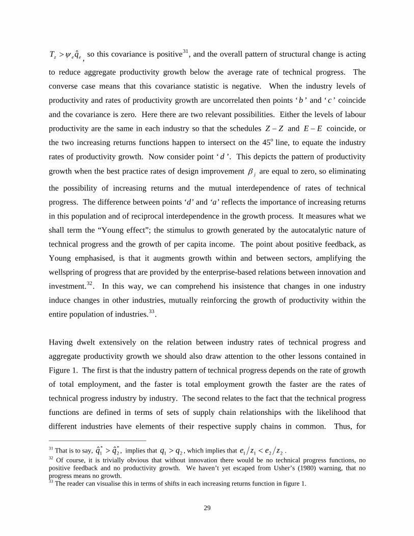
eez qT ˆψ> , so this covariance is positive31, and the overall pattern nge is acting
to reduce aggregate productivity growth below the average rate f technical progress. The
converse case means that this covariance statistic is negative. When the industry levels of
productivity and rates of productivity growth are uncorrelated then points ‘b ’ and ‘ c ’ coincide
and the covariance is zero. Here there are two relevant possibilities. Either the levels of labour
productivity are the same in each industry so that the schedules
of structural cha
o
ZZ − and EE − coincide, or
the two increasing returns functions happen to intersect on the 45o line, to equate the industry
rates of productivity growth. Now consider point ‘ d ’. This depicts the pattern of productivity
growth when the best practice rates of design improvement jβ are equal to zero, so eliminating
the possibility of increasing returns and the mutual interdependence of rates of technical
progress. The difference between points ‘d’ and ‘a’ reflects the importance of increasing returns
in this population and of reciprocal interdependence in the growth process. It measures what we
shall term the “Young effect”; the stimulus to growth generated by the autocatalytic nature of
technical progress and the growth of per capita e
phasised, is that it augments growth
ve elements of their re on. Thus, for
incom . The point about positive feedback, as
Young em
within and between se
spective supply chains in comm
ctors, amplifying the
wellspring of progress that are provided by the enterprise-based relations between innovation and
investment.32. In this way, we can comprehend his insistence that changes in one industry
induce changes in other industries, mutually reinforcing the growth of productivity within the
entire population of industries.33.
Having dwelt extensively on the relation between industry rates of technical progress and
aggregate productivity growth we should also draw attention to the other lessons contained in
Figure 1. The first is that the industry pattern of technical progress depends on the rate of growth
of total employment, and the faster is total employment growth the faster are the rates of
technical progress industry by industry. The second relates to the fact that the technical progress
functions are defined in terms of sets of supply chain relationships with the likelihood that
different industries ha
say, , implies that , which imp at 31 That is to *
2*1 ˆˆ qq > 21 qq > 1e 22 ze1z < . lies th
32 Of course, it is trivially obvious that without innovation there would be no technical progress functions, no positive feedback and no productivity growth. We haven’t yet escaped from Usher’s (1980) warning, that no progress means no growth. 33 The reader can visualise this in terms of shifts in each increasing returns function in figure 1.
29
example, an improvement in steel or plastics technology will influence the increasing returns
functions of all the vertically integrated industries that utilise steel and plastics in their supply
chains. Such a technological breakthrough of a “general purpose” kind will shift outwards both
the increasing returns functions in Figure 1, and induce further technical progress, according to
the pattern of weights `ju
Notice carefully, that Figure 1 represents a process of growth co-ordination at a point in time. It
’ and
’ are continually “on the move” as the relative employment shares vary over time
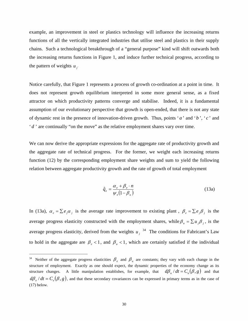
We can now derive the appropriate expressions for the aggregate rate of productivity growth and
e aggregate rate of technical progress. For the former, we weight each increasing returns
employmen
does not represent growth equilibrium interpreted in some more general sense, as a fixed
attractor on which productivity patterns converge and stabilise. Indeed, it is a fundamental
assumption of our evolutionary perspective that growth is open-ended, that there is not any state
of dynamic rest in the presence of innovation-driven growth. Thus, points ‘ a ’ and ‘b ’, ‘ c
d . ‘
th
function (12) by the corresponding employment share weights and sum to yield the following
relation between aggregate productivity growth and the rate of growth of total t
)( ue
eeq
βe n
ψ⋅α β
−+
=ˆ (13a)
In (13a), e
1
jje αα ∑= is the average rate improvement to existing plant , e jje ββ ∑= is the
average pro ress elasticity constructed with the employment shares, whileg jju u ββ ∑=
The conditions for Fabricant’s Law
, is the
average p ticity, derived from the weights 34 rogress elas
to hold in the aggregate are
ju
1<eβ , and 1<uβ , which are certainly satisfied if the individual
34 Neither of the aggregate progress elasticities eβ and uβ are constants; they vary with each change in the structure of employment. Exactly as one should expect, the dynamic properties of the economy change as its structure changes. A little manipulation establishes, for example, that ( gCdtd uu ,/ )ββ = and that
( gCdtd ee ,/ )ββ = , and that these secondary covariances can be expressed in primary terms as in the case of (17) below.
30

rates of best practice design improvement are less th n unity. Then we are assured that growth is
autocatalytic, with demand, output and productivity growth mutually reinforcing one another.
a
o derive the average rate of technical progress, , we net out the contribution of structural
change to productivity growth by multiplying ing returns function by the capacity
output weights , to obtain the relation35
zT
each increas
jz
T
( ) ( ) nT wez
wz ⎥
⎤⎢⎡
++⎥⎤
=ββ
β (13 ) neue
ez
⎦⎣ −⎦⎢⎣
⎡−
+βψβψ
βαα
11b
is rather a derived consequence of the difference between aggregate output
rowth and aggregate productivity growth. Rearranging (13a) we can thus express Young’s Law
egate relation between pr
output growth, thus
Where jjz z ββ ∑= and ∑= jjw w ββ are appropriately weighted best practice elasticities36.
The formulations in equations (13) map directly into Figure 1 because they take as given the rate
of employment growth. However, from our viewpoint the rate of growth of employment is not
an arbitrary given but
g
across the ensemble of industries, as the aggr oductivity growth and 37
( ) eue
zeee
gq
ββψβα
+−+
=1
ˆ (14)
35 Summing each technical progress function by the output shares gives . The rate of growth of productivity is eliminated using (13a)
ewzzz qnT ˆ* ββα ++=
36The weights jjj zw ψ= measure the contribution that each industry makes to the output weighted income
elasticity of demand, remembering that 1=zψ . We can always reduce a difference between the differently
weighted means of a variable to an appropriate covariance Thus, for example, ( ) ( )jjeeze qCq ααα ,=− expresses the difference between the different weighted averages for the industry rates of improvement. Similarly,
( ) ( )jje qCezeq βββ ,=− and ),( jjw zz C βψββ =− . If desired, the reader can rewrite (13b) in terms of various covariances to eliminate all the averages except those constructed using the employment weights. 37 An analogous expression in terms of the aggregate growth rate of output can be derived for (13b)
31

Equation (14) is the aggregate increasing returns function for this population of industries. It
reflects the implicit growth of knowledge and its rate of application industry by industry, and it
captures the fundamental point that average productivity growth cannot be independent of the
ructure of the ensemble of industries and how that structure is changing. The economy is
onomies must be. We shall
ke up the restless theme in our final section but we must turn first to the interdependence
st
simultaneously co-ordinated and restless, as all knowledge-based ec
ta
between aggregate output growth and aggregate productivity growth38.
VI. Closing the System: Accumulation and Increasing Returns.
We have shown how productivity growth differences at the industry level and the aggregate rate
of productivity growth are simultaneously determined. However, we have yet to determine what
the aggregate rate of output and productivity growth will be, for the individual industry growth
rates are ultimately constrained by the requirement that aggregate investment is equal to
ggregate saving. That is to say, there are limits to the exploitation of increasing returns and
a
these are naturally set by limits to the aggregate growth of the market. As Kaldor (1982),
pointed out there is a missing element in the Young approach that can only be dealt with by an
explanation of the relation between capital accumulation and effective demand in the aggregate.
38 Technical progress has such a powerful effect on some relative prices, that the reader may rightly wonder how the results are changed if we give pure substitution affects a more explicit role. Briefly, we can state that the full analysis of relative price effects requires that (3) be replaced by )ˆˆ(ˆ zk
kjkejj ppqng −−+= ∑χψ , where the
jkχ are the own and cross (pure) price substitution elasticities of demand for industry j with respect to each
industry price, the are the proportional rates of change in the industry prices, and is the rate of
change in the average price level- the standard of value. The aggregate income equals expenditure constraint and homogeneity ensure that the elasticities “add up” to give
kp kk
kz pzp ˆˆ ∑=
eqn ˆzg += , so that the relative price effects net out to
zero in the aggregate. That is to say, for the effect of changes in the price of industry i on all the
industries, and for the effect of changes in all prices on the demand for industry i . To elaborate the
deeper consequences, requires a theory of price formation at the industry level and this is why we do not take the discussion any further here. However, if one assumes that the dominant factor in changing prices is technical progress then one could, for example, approximate and set
0=∑k
kikz χ
0=∑k
ikχ
kqkp −= and find that the analysis of figure 1 is reproduced but with the slopes and positions of the Q schedules depending on the own and cross price substitution elasticities as well as on the income elasticities.
32

To express this more formally, relation (14) provides only one relation to determine two
unknowns. A relation is missing and here there are at least two possibilities. The first is to claim
that the rate of growth of employment, n , is given by virtue of arguments in relation to the
growth of population, labour migration, changing gender composition of the population, and
changes in institutional rules in relation to the market for labour. Whatever the rationale, the full
employment value of ‘ n ’ determines eq through (13a) and correspondingly determines the
growth rate of output, zg . This is the route explicitly followed by Arrow (1962) and Jones
(1995a and b) in their very different accounts of endogenous growth, for they both end up with
the claim that steady state productivity growth is proportional to the growth in population.
Consequently, a stationary population implies an end to progress which seems an unduly tough
restriction on the growth of knowledge and its transfer into the growth of productivity. Instead
we follow a different approach; one grounded in Harrod’s pioneering treatment of endogenous
rowth in terms of aggregate saving and investment. In this view, the requirements for
ng r.39
We start by assuming that all profits are distributed, all investment is funded via the capital
capacity output is then equal to where
g
macroeconomic co-ordination set the aggregate constraints on the relations between growth rates
at industry level. In following this approach, some hypothesis has to be adopted on the nature of
capital markets, investment and savi behaviou
market, and that the aggregate saving ratio of households is a constant, s 40.The ratio of saving to
zsx ∑= jjz xzx is the average degree of capacity
that aggregate saving ratio must equal the aggregate investment ratio for the economy but here
we must introduce the two kinds of investment that we alluded to in constructing each technical
utilisation and jx is the degree of capacity utilisation (the ratio of actual to capacity output) in
each industry. Long run normal prices are set to keep each industry operating at full capacity,
1== zj xx , and thus ensure that the rate of growth of capacity is equal to the rate of growth of
demand, given each industry’s propensity to invest. Coordination of the capital market requires
39 The Harrod model is a more sophisticated version of the so-called AK model of endogenous growth, by virtue of having an independent investment function. The crucial change introduced by Solow’s growth model was not the assumption of a variable capital output ratio but rather the disappearance of an independent investment function. It is Say’s law model in which savings and investment are automatically equal in all economic circumstances. See Kurz and Salvadori (1998) for an elaboration and critique. Other, post-Keynesian, approaches differentiating savings by type of income are equally applicable but would take us too far afield in this preliminary exposition. 40 As noted above, this is tantamount to assuming a unitary income elasticity of demand for per capita wealth.
33

progress func
in each industry, the ratio of this kind of investment to the industry’s output is
. It follows that the aggregate ratio of capacity expanding investment to capacity
tion. First there is investment that expands capacity. Since capacity is fully
employed
( ) j gbQI =/
is given by
jj
vzjjjQ
jjv gvg ∑= is the rate of growth of the aggregate capital stock, defined using the weights
jjzj bzbv = . The weights jv measure the share of each industry in the total capital stock which
is equal to the proportionate contribution that each industry makes to the aggregate capital output
ratio. Secondly there is improvement investment that enhances the efficiency with which current
capacity is operat
gbgbzI=∑=
d, an
where
e d we let μ denote the aggregate ratio of this kind of investment to
ding investment.41 From this, we immediately obtain a version of the familiar
ition
capacity expan
d ond
Harro c
( ) zv bμ+1
Given our assumptions about capacity utilization rates, this is the familiar Harrod formula, taking
account of the distinction between the two kinds
sg = (15a)
of investment. Clearly, the greater the fraction
t is devoted to improvement rather than capacity expansion, the smaller will be
ould only be equivalent in conditions of proportional growth, that is,
hen growth is not associated with development, but here they are logically different and are
related by the condition
of investment tha
the rate of growth of the aggregate capital stock.
However, vg in this formula is not the growth rate of aggregate capacity output as normally
defined, which is, jjz gzg ∑= , the output share weighted average of the industry growth rates.
The two growth rates w
w
41 The distinction was first made by Harrod, (1946, p.79).
34
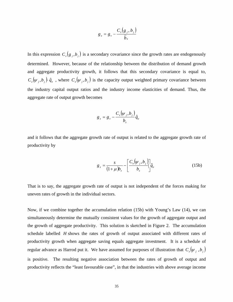
( )
zvz b
In this expression
jjz bgCgg
,−=
( )jjz bgC , is a secondary covariance since the growth rates are endogenously
owever, f the relationship between the distribution of demand growth
and aggregate productivity growth, it follows that this secondary covariance is equal to,
determined. H se obecau
( ) ejjz qbC ˆ, ⋅ψ , where ( )jjz bC ,ψ is the capacity output weighted primary covariance between
e industry capital output ratios and the industry income elasticities of demand. Thus, the
aggregate rate of output growth becomes
th
( )e
zvz b
jjz qbC
gg ˆ,ψ
−=
nd it follows that the aggregate growth rate of output is related to the aggregate growth rate of
productivity by
a
( )( )
ezz
z bb1 ⎦⎣+ μ
jje qbCsg ˆ
,⎥⎤
⎢⎡
−=ψ
(15b)
hat is to say, the aggregate growth rate of output is not independent of the forces making for
rm
T
uneven rates of growth in the individual sectors.
Now, if we combine together the accumulation relation (15b) with Young’s Law (14), we can
simultaneously dete ine the mutually consistent values for the growth of aggregate output and
the growth of aggregate productivity. This solution is sketched in Figure 2. The accumulation
schedule labelled H shows the rates of growth of output associated with different rates of
productivity growth when aggregate saving equals aggregate investment. It is a schedule of
regular advance as Harrod put it. We have assumed for purposes of illustration that ( )jjz bC ,ψ
is positive. The resulting negative association between the rates of growth of output and
productivity reflects the “least favourable case”, in that the industries with above average income
35
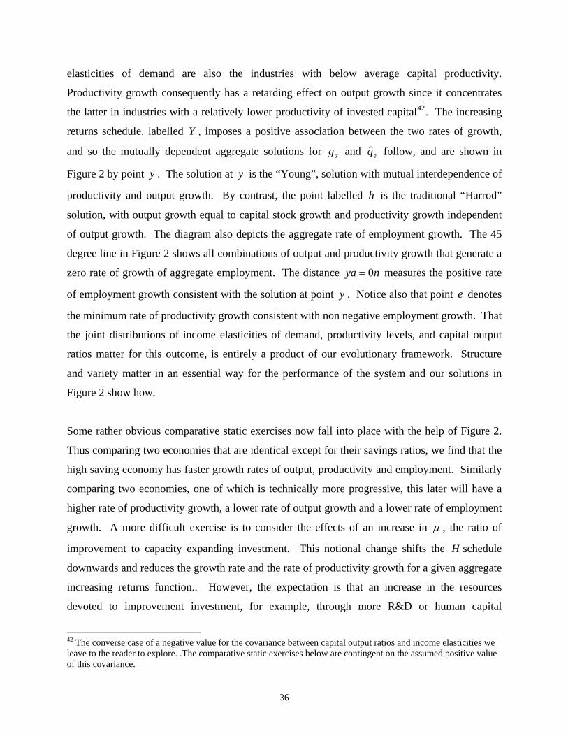
elasticities of demand are also the industries with below average capital productivity.
Productivity growth consequently has a retarding effect on output growth since it concentrates
the latter in industries with a relatively lower productivity of invested capital42. The increasing
returns schedule, labelled Y , imposes a positive association between the two rates of growth,
and so the mutually dependent aggregate solutions for zg and e follow, and are shown in
Figure 2 by point
q
y . The solution at y is the “Young”, solution with mutual interdependence of
productivity and output growth. By contrast, the point labelled h is the traditional “Harrod”
solution, with output growth equal to capital stock growth and productivity growth independent
of output growth. The diagram also depicts the aggregate rate of employment growth. The 45
degree line in Figure 2 shows all combinations of output and productivity growth that generate a
zero rate of growth of aggregate employment. The distance nya 0= measures the positive rate
of employment growth consistent with the solution at point y . Notice also that point e denotes
the minimum rate of productivity growth consistent with non negative employment growth. That
the joint distributions of income elasticities of demand, productivity levels, and capital output
ratios matter for this ou e, is entirely a pro framework. Structure
nd variety matter in an essential way f r the performa and our s lutions in
tcom duct of our evolutionary
a o nce of the system o
Figure 2 show how.
Some rather obvious comparative static exercises now fall into place with the help of Figure 2.
Thus comparing two economies that are identical except for their savings ratios, we find that the
high saving economy has faster growth rates of output, productivity and employment. Similarly
comparing two economies, one of which is technically more progressive, this later will have a
higher rate of productivity growth, a lower rate of output growth and a lower rate of employment
growth. A more difficult exercise is to consider the effects of an increase in μ , the ratio of
improvement to capacity expanding investment. This notional change shifts the H schedule
downwards and reduces the growth rate and the rate of productivity growth for a given aggregate
increasing returns function.. However, the expectation is that an increase in the resources
devoted to improvement investment, for example, through more R&D or human capital
42 The converse case of a negative value for the covariance between capital output ratios and income elasticities we leave to the reader to explore. .The comparative static exercises below are contingent on the assumed positive value of this covariance.
36

formation, will also shift this schedule to the right, increasing the rate of productivity growth but
further reducing the rate of output growth. How this works out will depend on how the
investments pay off in terms of improved productivity growth, and this is a question that can
only be addressed industry by industry and firm by firm. This is beyond our remit but at least we
now where to look to see how investments in knowledge generation are translated into
development and growth, and the relation between the
ifferent stylised facts? The discussion is necessarily brief but we hope that it points to deeper
k
additional wealth, and it is not at the macroeconomic level.
The pattern of co ordination in Figure 2 represents a perfectly plausible “model” of evolutionary
growth without making any assumptions that the point of coordination is a stable long run
attractor for the economy. Quite the contrary, what makes this approach evolutionary is that the
determinants of the point of coordination are restless; they evolve in response to the structural
changes that are induced by the processes of economic coordination at aggregate and industry
levels. It is not a system in equilibrium; indeed, capitalism in equilibrium seems from this point
of view a contradiction in terms. There are always reasons and incentives to change prevailing
arrangements, and every change opens up new opportunities for further change, ad infinitum.
This is the powerful message first stated by Smith, refined by Marshall and Young, and given
empirical content by Fabricant, Schumpeter, Kaldor and modern evolutionary economists. What
can we say on the nature of restless
d
questions about evolutionary growth.
VII. Restless Capitalism and the Stylised Facts
We begin by reminding ourselves of the basic dynamics of structural change. An industry is
increasing its share of aggregate output precisely to the degree that its income elasticity of
demand exceeds a value of unity, the population average income elasticity. Nothing more needs
to be said, but when we come to the changes in employment shares, the outcome is s
transparent, for employment and output shares do not automatically move in step. An industry is
increasing its share of employment if nn j > which is equivalent to the requirement, jje qq ˆˆ >
a little les
ψ .
That is to say, the ratio of industry to average productivity growth has to be less than the income
37
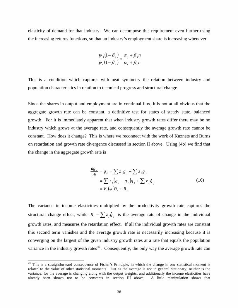
elasticity of demand for that industry. We can decompose this requirement even further using
the increasing returns functions, so that an industry’s employment share is increasing whenever
( )( ) n
n
ee
jj
ue
jj
βαβα
βψβψ
+
+>
−
−
11
This is a condition which captures with neat symmetry the relation between industry and
population characteristics in relation to technical progress and structural change.
Since the shares in output and employment are in continual flux, it is not at all obvious that the
aggregate growth rate can be constant, a definitive test for states of steady state, balanced
growth. For it is immediately apparent that when industry growth rates differ there may be no
industry which grows at the average rate, and consequently the average growth rate cannot be
onstant. How does it change? This is where we reconnect with the work of Kuznets and Burns
on retardation and growth rate divergence discussed in section II above. Using (4b) we find that
the change in the aggregate growth rate is
c
( )ze
jjjzjj
Rq
gzgggz
+
+−= ∑ ∑ˆ
& (16)
The variance in income elasticities multiplied by the productivity growth rate captures the
structural change effect, while
( )z
jjjjzz
V
gzgzgdt
dg
=
+== ∑ ∑
ψ
&&&
∑= jjz gzR ˆ is the average rate of change in the individual
growth rates, and measures the retardation effect. If all the individual growth rates are constant
this second term vanishes and the average grow rate is necessarily increasing because it is
th
converging on the largest of the given industry growth rates at a rate that equals the population
variance in the industry growth rates43. Consequently, the only way the average growth rate can
43 This is a straightforward conseque ple, in
l moments. along with th
not to be constants in section III above. A little manipulation shows that
nce of Fisher’s Princi which the change in one statistical moment is related to the value of other statistica Just as the average is not in general stationary, neither is the variance, for the average is changing e output weights, and additionally the income elasticities have already been shown
38

remain constant is if the individual growth rates are declining, that is to say that the
Kuznets/Burns retardation principle holds on average. If it should happen that the average
output growth rate is indeed constant then the required average rate of retardation is given
by ( ) ezz qVR ˆψ−= , which increases with the average rate of productivity growth. Thus the
Kuznets ad Burns analysis of individual industries has its aggregate counterpart in (15)44.
Principal among the aggregate stylised facts is the constancy over time of the aggregate capital
output ratio. Within our framework there is no necessity for it to be constant since the given
capital output ratios differ industry by industry. Consequently the aggregate capital output ratio
evolves with the output structure according to the relation
( )e
z
jjzzvz q
bbC
ggb ˆ,ˆ ⎥
⎦
⎤⎢⎣
⎡=−=
ψ (17a)
Only if the distributions of capital output ratios and income elasticities of demand are
uncorrelated at the prevailing output structure will the aggregate capital output ratio be constant.
This is an important clue to the nature of the evolutionary process; its aggregate consequences
are conditional not only on the variety within the fundamental data of the economy but on their
degree of correlation as well. Thus, as a general rule in an evolving economy, Harrod neutrality
at industry level will not produce Harrod neutrality at the aggregate economy level, and the
purpose of the aggregation procedure is to identify how and why the emergent aggregate
properties do not mimic the corresponding properties at industry level. Of course, Figure 2
( ) ( ) ( )z CS
dVψψψ
ψ&,2+= . In this expression, jjzjzdt
( )jzS ψ is the third moment of the income elasticities
heir population average, and ( )jjzC ψ ψaround t &, is the output weighted covariance between the elasticities and their rates of change. 44 The reader can work through the consequences for other aggregate growth rates, for example the growth rate of the capital stock, . Because jjK gvg ∑= `ˆ KKI ggg −= it follows that the rate of change of the aggregate
accumulation rate can be expressed as ( ) ( )⎥
⎦
⎤⎢⎣
⎡+−= jve
z
jjzK gVq
kbC
g ˆ,
ˆψ
. In this expression, ( )jv gV is the
variance of the industry capital stock growth rates constructed using each industry’s share in the aggregate capital stock as weights. This variance effect reduces the growth rate of the capital stock but the covariance term may work either way. In figure 2, the two effects are in the same direction since the covariance is there assumed to be positive.
39
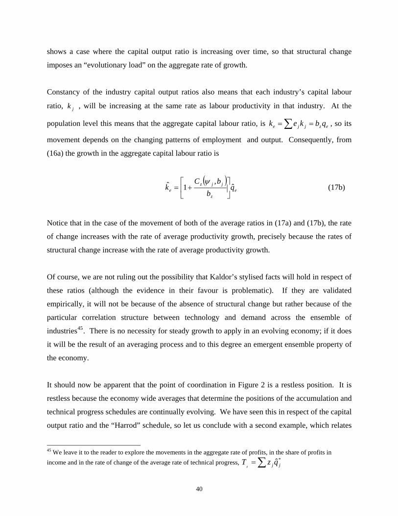
shows a case where the capital output ratio is increasing over time, so that structural change
imposes an “evolutionary load” on the aggregate rate of growth.
ratio, jk , will be increasing at the same rate as labour productivity in that industry. At the
Constancy of the industry capital output ratios also means that each industry’s capital labour
opul n level this means that the aggregate capital labour ratio, is , so its
movement depends on the changing patterns of employment and output. Consequently, from
(16a) the growth in the aggregate capital labour ratio is
atio ∑ == ezjje qbkekp
( )e
z
jjze q
bbC
k ˆ,
1ˆ ⎥⎦
⎤⎢⎣
⎡+=
ψ (17b)
Notice that in the case of the movement of both of the average ratios in (17a) and (17b), the rate
relation structure between technology and demand across the ensemble of
dustries45. There is no necessity for steady growth to apply in an evolving economy; if it does
n
of change increases with the rate of average productivity growth, precisely because the rates of
structural change increase with the rate of average productivity growth.
Of course, we are not ruling out the possibility that Kaldor’s stylised facts will hold in respect of
these ratios (although the evidence in their favour is problematic). If they are validated
empirically, it will not be because of the absence of structural change but rather because of the
particular cor
in
it will be the result of an averaging process and to this degree an emergent ensemble property of
the economy.
It should now be apparent that the point of coordination in Figure 2 is a restless position. It is
restless because the economy wide averages that determine the positions of the accumulation and
technical progress schedules are co tinually evolving. We have seen this in respect of the capital
output ratio and the “Harrod” schedule, so let us conclude with a second example, which relates
45 We leave it to the reader to explore the movements in the aggregate rate of profits, in the share of profits in income and in the rate of change of the average rate of technical progress, ∑= *ˆ jj qz
zT
40

to the change in the “Young” schedule. Consider then the change in the average rate of
improvement on existing plants, eα . This is a more complicated story. The rate at which this
verage changes has two components, one reflecting the impact of the changing employment
(accelerations of decelerations) in the industry
specific rates of improveme ting plants and capital structures,
a
structure, and the other reflecting any changes
nt in exis jα . Thus
∑ ∑+== jjjjee ee
dtd
αααα
&&&
rm we have little to say, since it is a sum of changes arising below the
industry level and is ruled out of our discussion for this reason. However, the structural effect in
the first term is far more amenable to analysis. By familiar steps it follows immediately that
About the second te
( )∑ = jjejj nCe ,αα& . If this covariance is positive then the employ structure is ment
those industries with above average rates of improvement,
the population average rate of improvement. Taking account of the fact
ployment growth rates around their average, , is equal to
increasingly concentrated on
ecessarily increasing
that the distribution of the em
jej qq ˆˆ −
n
nn j −
ψ , it follows that
( ) ( ) ( )jjeejjeje qCqCnC ˆ,ˆ,j , αψαα −⋅=
This is a typical product of evolutionary economic reasoning, in that the covariation between an
endogenous variable (in this case jn ) and an exogenous variable (in this case jα ) reflects the
deeper causal structure underlying the changing patterns of output and employment. This deeper
structure is reflected in the covariation between income elasticities and rates of improvement and
between rates of productivity growth and rates of improvement. The system is restless because
of the variety contained within it and because of the correlation between those different
dimensions of economic variety. All is flux, the product of variation, selection and the ongoing
41

development of productivity within the causal structure of dema46
nd and output co ordination,
industry by industry and in the aggregate .
VIII. Concluding Remarks.
When the uneven growth of the economy is driven by and drives the uneven growth of useful
human knowledge, we can neither restrict our analysis of growth to the aggregate economy nor
can we treat structural change as a passive epiphenomenon. Innovation and technical progress
cause and are caused by the patterns of economic restructuring and differential growth in the
economy. At its most fundamental level the system evolves because of the non representative
behaviours contained within it. Unfortunately, a full treatment of the origins of wealth from
knowledge must necessarily delve below the level of the industry to the connections between
innovation and the competitive performance of rival firms. This further step will reinforce our
claim that capitalism is restless because knowledge is restless; that capitalism grows unevenly
because knowledge grows unevenly, precisely what Schumpeter meant by creative destruction.
Diversity and correlation of determining characteristics are the keys to adaptive, restless
capitalism; and it is the diversity in the conditions of technical progress, in capital output ratios,
and in income elasticities of demand that we have shown to sustain the essential unity of our two
sets of stylised facts. Aggregate growth and structural self-transformation are one and the same
roblem. Needless to add, in an open economy these evolutionary forces are further amplified
trade and investment, although that really must be another story.
p
through international
Acknowledgments
46 The reader can go further and eliminate the endogenous productivity growth rates in )ˆ,( jje qC α by using the
rns functions (12). After some manipulation, using the different weighting schemes introduced ove, we find that this is reduced to the rather complicated but readily intelligible expression
inab
creasing retu
[ ]( ) ( ) ( ) ( ) ( )( ) jjuenjjeejjejejje CCqnCVnC βαψβαψβαα ,1,ˆ,,α − −+−−= . A special case arises
when the primary elements, α , β , ψ , are uncorrelated one with the other. Then this expression reduces to
( ) ( )jeje VnC α α−=,, , the latter being the employment weighted variance in the rates of improvement. In this case, the effects of structural change result in a decline in the average rate of improvement.
42

This paper is an extension and revision of Metcalfe, Foster and Ramlogan, 2006. We thank
the generous support of Curtin
Cristiano Antonelli, Harry Bloch, Dick Nelson, and Mark Setterfield for their comments and
suggestions on earlier drafts. JSM gratefully acknowledges
University and its School of Economics and Finance, where much of the initial drafting was
carried out.
References
Abramovitz, M., 1989, Thinking about Economic Growth: and other Essays on Economic
Growth and Welfare, Cambridge, Cambridge University Press
Acemoglu, D., and Guerrieri,V., 2008, ‘Capital Deepening and Nonbalanced Economic Growth’,
Journal of Political Economy, Vol.116(3), pp.467-498.
Aldrich, H.E., Hodgson, G.M., Hull, D.L., Knudsen, T., Mokyr, J., and Vanberg, V.,. 2008, ‘In
Defence of Generalised Darwinism’, Journal of Evolutionary Economics, Vol. 18, pp. 577-596.
Amendola, M., and Gaffard, J.L., 1988, The Innovative Choice, Oxford, Blackwell.
Amendola, M., and Gaffard, J.L., 1998, Out of Equilibrium, Oxford, Oxford University Press.
Andersen, E.S., 2004, ‘Population Thinking, Price’s Equation and the Analysis of Economic
Evolution’, Evolutionary and Institutional Economics Review, Vol. 1, pp. 127-148.
Arrow, K.J., 1962, ‘The Economic Implications of Learning by Doing’, Review of Economic
Studies, Vol. 29, pp. 155-173.
Bairam, E.I., 1987, ‘The Verdoorn Law, Returns to Scale and Industrial Growth: A Review of
the Literature’, Australian Economic Papers, Vol. 26, pp. 20-42.
and Productivity Growth’, Baldwin, J.R. and Gu, W., 2005, ‘Competition, Firm Turnover
mimeo, Ottowa, Micro Economic Analysis Division, Statistics Canada.
Bartelsman, E. J., and Doms, M., 2000, ‘Understanding Productivity: Lessons from Longitudinal
Data’, Journal of Economic Literature, Vol. 38, pp. 569-594.
Baumol, W.J., Blackman, S.A.B. and Wolff, E.N., 1989, Productivity and American Leadership,
MIT Press.
Bianchi, M. (ed.), 1998, The Active Consumer, Routledge, London.
Bliss, C., 1975, Capital Theory and the Distribution of Income, Elsevier, New York.
ral Composition in
Advanced Economies, Structural Change and Economic Dynamics
Bonatti, L., and Felice, G., 2008, ‘Endogenous Growth and Changing Secto
, Vol. 19, pp. 109-131.
43

Burns, A.F., 1934, Production Trends in the United States Since 1870, Boston, NBER.
Carlin, W., Haskel, J. and Seabright, P., 2001, ‘Understanding ‘The Essential Fact About
Capitalism’: Markets, Competition and Creative Destruction’, National Institute Economic
Review, No. 175, pp. 67-84.
Clark, C., 1944, The Conditions of Economic Progress, London, Macmillan.
Cornwall, J. and Cornwall, W., 2002, ‘A Demand and Supply Analysis of Productivity Growth’,
Structural Change and Economic Dynamics, Vol. 13, pp. 203-230.
Disney, R., Haskel, J. and Heden, Y., 2003, ‘Restructuring and Productivity Growth in UK
Manufacturing’, Economic Journal, Vol. 113, pp. 666-694.
Dosi, G., 2000, Innovation, Organisation and Economic Dynamics, Cheltenham, Edward Elgar.
Echevarria, C., 1997, ‘Changes in Sectoral Composition Associated with Economic Growth’,
International Economic Review, Vol. 38(2), pp.431-452.
Eltis, W., 1973, Growth and Distribution, London, Macmillan.
Fabricant, S., 1940, The Output of Manufacturing Industries: 1899-1937, New York, NBER,
Fabricant, S., 1942, Employment in Manufacturing: 1899-1937, New York, NBER.
h
Wisdom: Alternative Perspectives on the New
Fagerberg, J., and Verspagen, B., 1999, ‘Vision and Fact: A Critical Essay on the Growt
Literature’, in Madrick, J., (ed), Unconventional
Economy, New York, The Century Foundation Press.
Freeman, C. and Louça, C., 2001, As Time Goes By: From the Industrial Revolutions to the
Information Revolution, Oxford, Oxford University Press.
Foster, J., 2000, ‘Competitive Selection, Self-Organisation and Joseph A Schumpeter’, Journal
of Evolutionary Economics, Vol.10, pp.311-328.
Gaston, J.F., 1961, Growth Patterns in Industry: A Re-Examination, New York, National
Industrial Conference Board.
Harberger, A.C., 1998, ‘A Vision of the Growth Process’, American Economic Review, Vol. 88,
pp. 1-32.
Harcourt, G.C., 1972, Some Cambridge Controversies in the Theory of Capital, Cambridge,
Cambridge University Press.
Harrod, R.F., 1948, Towards a Dynamic Economics, London, Macmillan.
44

Hoffman, W.G., 1949, ‘The Growth of Industrial Production in Great Britain. A Quantitative
Survey’, Economic History Review, Vol.2, pp. 162-180.
Jones, C.I., 1995a, ‘Rand D-Based Models of Economic Growth’, Journal of Political Economy,
5b, ‘Time Series Tests of Endogenous Growth Models’, Quarterly Journal of
Vol. 103, pp. 759-804.
Jones, C.I., 199
Economics, Vol. 110, pp. 495-525.
Kaldor, N., 1957, ‘A Model of Economic Growth’, Economic Journal, Vol. 67, pp 591-624
ital
Kaldor, N., 1961,’Capital Accumulation and Economic Growth’, in F.A., Lutz and D.C., Hague,
(eds.), The Theory of Cap , London, Macmillan.
Kaldor, N., 1972, ‘The Irrelevance of Equilibrium Economics’, Economic Journal, Vol.82,
pp.1237-1255.
Kindleberger, C.P., 1989, Economic Laws and Economic History, The Raffaelle Mattioli
ynamics’ in The Ethics of Competition
Lectures, Cambridge, Cambridge University Press.
Knight, F.H., 1935 (1977), ‘Statics and D , Transactions
tor Distinction’, Journal of Economic Methodology
Publishers, New Jersey.
Knudsen, T. 2004, ‘General Selection Theory and Economic Evolution: The Price Equation and
the Replicator/Interac , Vol. 11, pp. 147-173.
Kuznets, S., 1929, Secular Movements of Production and Prices, Houghton Miflin, Boston.
Kongsamut, P., Rebelo, S., and Xie, D., 2001, ‘Beyond Balanced Growth’, The Review of
Economic Studies, 2001(4), pp.869-882.
Kurz, H. and Salvadori, N., 1998, ‘The “New” Growth Theory: Old Wine in New Goatskins’, in
Coricelli, F., Di Matteo, M. and Hahn, F. (eds.), New Theories in Growth and Development,
MacMillan, London.
Kurz, H., 2008, ‘On the Growth of Knowledge about the Role of Knowledge in Economic
Growth’, mimeo, University of Graz.
Kuznets, S., 1954, Economic Change, Heinemann, London.
Kuznets, S., 1971, Economic Growth of Nations, Belknap, Harvard.
Kuznets, S., 1977, ‘Two Centuries of Economic Growth: Reflections on US Experience’,
American Economic Review, Vol. 67, pp. 1-14.
Laitner, J., 2000, ‘Structural Change and Economic Growth’, Review of Economic Studies,
Vol.67(3),pp.545-561.
45
Landes, D.S., 1967, The Unbound Prometheus, Cambridge, Cambridge University Press.
Maddison, A., 1991, Dynamic Forces in Capitalist Development, Oxford, Oxford University
Press.
Marshall, A., 1919, Industry and Trade, London, Macmillan.
Marshall. A., 1920, Principles of Economics, 8th (Variorum) edition, London, Macmillan.
McCombie, J.S.L. 1986, ‘On Some Interpretations of the Relationship Between Productivity and
Output Growth’, Applied Economics, Vol.18, pp.1215-1225.
Metcalfe, J.S., 1998, Evolutionary Economics and Creative Destruction, London, Routledge.
Metcalfe, J.S., 2001, ‘Institutions and Progress’, Industrial and Corporate Change, Vol.10,
pp.561-586.
J.S. Metcalfe, J. Foster and R. Ramlogan, 2006, ‘Adaptive Economic Growth’, Cambridge
Journal of Economics, Vol. 30, No. 1, pp.7-32.
the Measurement of Metcalfe, J.S, and Ramlogan, R., 2006, ‘Creative Destruction and
Productivity Change’, Revue, de L’OFCE, Paris, Observatoire Francais, des Conjunctures
nd the Population Method’,
Economiques, Presses de Science Po.
J.S. Metcalfe, 2008, ‘Accounting for Economic Evolution: Fitness a
Journal of Bioeconomics, Vol. 10, pp.23-50.
Mokyr, J., 1990 , The Lever of Riches, Oxford, Oxford University Press.
Mokyr, J., 2002, The Gifts of Athena, Princeton, Princeton University Press.
Montobbio, F., 2002, ‘An Evolutionary Model of Industrial Growth and Structural Change’,
Structural Change and Economic Dynamics, Vol.13(4),pp.387-414.
Nelson, R., Peck, M, and Kalachek, E.D., 1967, Technology, Economic Growth and Public
Policy, Washington, The Brookings Institution.
Nelson, R. and Winter, S., 1974, ‘Neoclassical vs. Evolutionary Theories of Economic Growth:
Critique and Prospectus’, Economic Journal, Vol. 84, pp. 886-905.
Nelson, R., and Winter, S., 1982, An Evolutionary Theory of Economic Change, Harvard,
and Production functions when Techniques are
Belknap Press.
Nelson, R., 1989, ‘Industry Growth Accounts
Idiosyncratic’, Journal of Economic Behaviour and Organisation, Vol.11, pp.323-341.
Nelson, R., 2005, Technology, Institutions and Economic Growth, Harvard, Harvard University
Press.
46

Ngai, L.R., and Pissarides, C.A., 2004, ‘Structural Change in a Multi-Sector Growth Model’,
mimeo, CEPR, London School of Economics.
Pasinetti, L.L., 1981, Structural Change and Economic Growth, Cambridge University Press.
Pasinetti, L.L., 1993, Structural Economic Dynamics, Cambridge University Press.
Salter, W.E.G., 1960, Productivity and Technical Change, Cambridge, Cambridge University
Press.
Saviotti, P., and Pyka, A., 2004, ’Economic Development by the Creation of New Sectors’,
Journal of Evolutionary Economics, Vol.14(1), pp.1-36.
Saviotti, P., 2001, ‘Variety, Growth and Demand’, Journal of Evolutionary Economics, Vol.
11(1), pp. 119-142.
ic Sayers, R.S., 1950, ‘The Springs of Technical Progress in Britain, 1919-1939’, Econom
Journal, Vol. 60, pp. 275-291.
Schumpeter, J.A., 1912 (1934) The Theory of Economic Development, Oxford, Oxford
University Press.
Schumpeter, J., 1928, ‘The Instability of Capitalism’, Economic Journal, Vol.38, pp.361-386. Scott, M. F.G., 1989, A New View of Economic Growth, Oxford University Press.
Silverberg, G., and Verspagen, B., 1998, ‘Economic Growth as an Evolutionary Process’, in, J.
Lesourne and A. Orlean, (eds), Advances in Self-Organisation and Evolutionary Economics,
Economica, Paris.
Stigler, G.J., 1947, Trends in Output and Employment, NBER, New York.
Steedman, I., 2003, ‘On Measuring Knowledge in New (Endogenous) Growth Theory’, in
AssessmentH.Kurz and N.Salvadori, (eds) Old and New Growth Theories an , Cheltenham,
9, Main Currents in Cumulative Causation
Edward Elgar.
Toner, P., 199 , London, Macmillan Press.
Usher, D., 1980, The Measurement of Economic Growth, Blackwell, London.
Witt. U., 2003, The Evolving Economy, Cheltenham, Edward Elgar.
Young, A.A., 1928, ‘Increasing Returns and Economic Progress’, Economic Journal, Vol. 38,
pp. 527-42.
47

Figure 1
The Distributed Pattern of Technical Progress
2q
zT
eeqψ
2α
0
O45
d
1α eeqψ zT1q
c
1Q
2Q
Z
b
E
E
Z
O45
a
2q
zT
″1q
*1q
*2q
48

49
Figure 2
The Co-ordination of Aggregate Productivity
Growth, Output Growth and Employment Growth
g
Kg
zg
n
0eq eq
e
a
h
o45
y
Y
n 0=n
H