
Evolution strategies
26
Evolution strategies Chapter 4
-
Upload
mona-deleon -
Category
Documents
-
view
18 -
download
0
description
Evolution strategies. Chapter 4. ES quick overview. Developed: Germany in the 1970’s Early names: I. Rechenberg, H.-P. Schwefel Typically applied to: numerical optimisation Attributed features: fast good optimizer for real-valued optimisation relatively much theory Special: - PowerPoint PPT Presentation
Transcript of Evolution strategies

Evolution strategies
Chapter 4

A.E. Eiben and J.E. Smith, Introduction to Evolutionary ComputingEvolution Strategies
ES quick overview
Developed: Germany in the 1970’s Early names: I. Rechenberg, H.-P. Schwefel Typically applied to:
– numerical optimisation Attributed features:
– fast– good optimizer for real-valued optimisation– relatively much theory
Special:– self-adaptation of (mutation) parameters standard

A.E. Eiben and J.E. Smith, Introduction to Evolutionary ComputingEvolution Strategies
ES technical summary tableau
Representation Real-valued vectors
Recombination Discrete or intermediary
Mutation Gaussian perturbation
Parent selection Uniform random
Survivor selection (,) or (+)
Specialty Self-adaptation of mutation step sizes
A.E. Eiben and J.E. Smith, Introduction to Evolutionary ComputingEvolution Strategies
Introductory example
Task: minimimise f : Rn R Algorithm: “two-membered ES” using
– Vectors from Rn directly as chromosomes– Population size 1– Only mutation creating one child– Greedy selection
A.E. Eiben and J.E. Smith, Introduction to Evolutionary ComputingEvolution Strategies
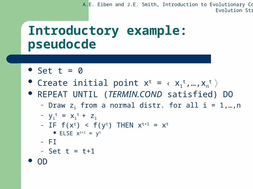
Introductory example: pseudocde
Set t = 0 Create initial point xt = x1
t,…,xnt
REPEAT UNTIL (TERMIN.COND satisfied) DO– Draw zi from a normal distr. for all i = 1,…,n– yi
t = xit + zi
– IF f(xt) < f(yt) THEN xt+1 = xt
ELSE xt+1 = yt
– FI– Set t = t+1
OD

A.E. Eiben and J.E. Smith, Introduction to Evolutionary ComputingEvolution Strategies
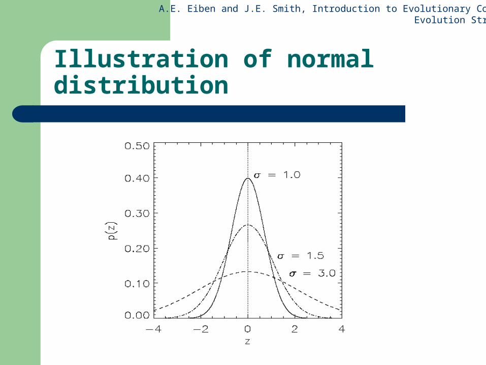
Introductory example: mutation mechanism
z values drawn from normal distribution N(,) – mean is set to 0 – variation is called mutation step size
is varied on the fly by the “1/5 success rule”: This rule resets after every k iterations by
= / c if ps > 1/5
= • c if ps < 1/5
= if ps = 1/5
where ps is the % of successful mutations, 0.8 c 1
A.E. Eiben and J.E. Smith, Introduction to Evolutionary ComputingEvolution Strategies
Illustration of normal distribution

A.E. Eiben and J.E. Smith, Introduction to Evolutionary ComputingEvolution Strategies
Another historical example:the jet nozzle experiment
Initial shape
Final shape
Task: to optimize the shape of a jet nozzleApproach: random mutations to shape + selection
A.E. Eiben and J.E. Smith, Introduction to Evolutionary ComputingEvolution Strategies
Representation
Chromosomes consist of three parts:– Object variables: x1,…,xn
– Strategy parameters: Mutation step sizes: 1,…,n
Rotation angles: 1,…, n
Not every component is always present
Full size: x1,…,xn, 1,…,n ,1,…, k
where k = n(n-1)/2 (no. of i,j pairs)

A.E. Eiben and J.E. Smith, Introduction to Evolutionary ComputingEvolution Strategies
Mutation
Main mechanism: changing value by adding random noise drawn from normal distribution
x’i = xi + N(0,) Key idea:
is part of the chromosome x1,…,xn, is also mutated into ’ (see later how)
Thus: mutation step size is coevolving with the solution x

A.E. Eiben and J.E. Smith, Introduction to Evolutionary ComputingEvolution Strategies
Mutate first
Net mutation effect: x, x’, ’ Order is important:
– first ’ (see later how)– then x x’ = x + N(0,’)
Rationale: new x’ ,’ is evaluated in 2 ways– Primary: x’ is good if f(x’) is good – Secondary: ’ is good if the x’ it created is good
Reversing mutation order this would not work
A.E. Eiben and J.E. Smith, Introduction to Evolutionary ComputingEvolution Strategies
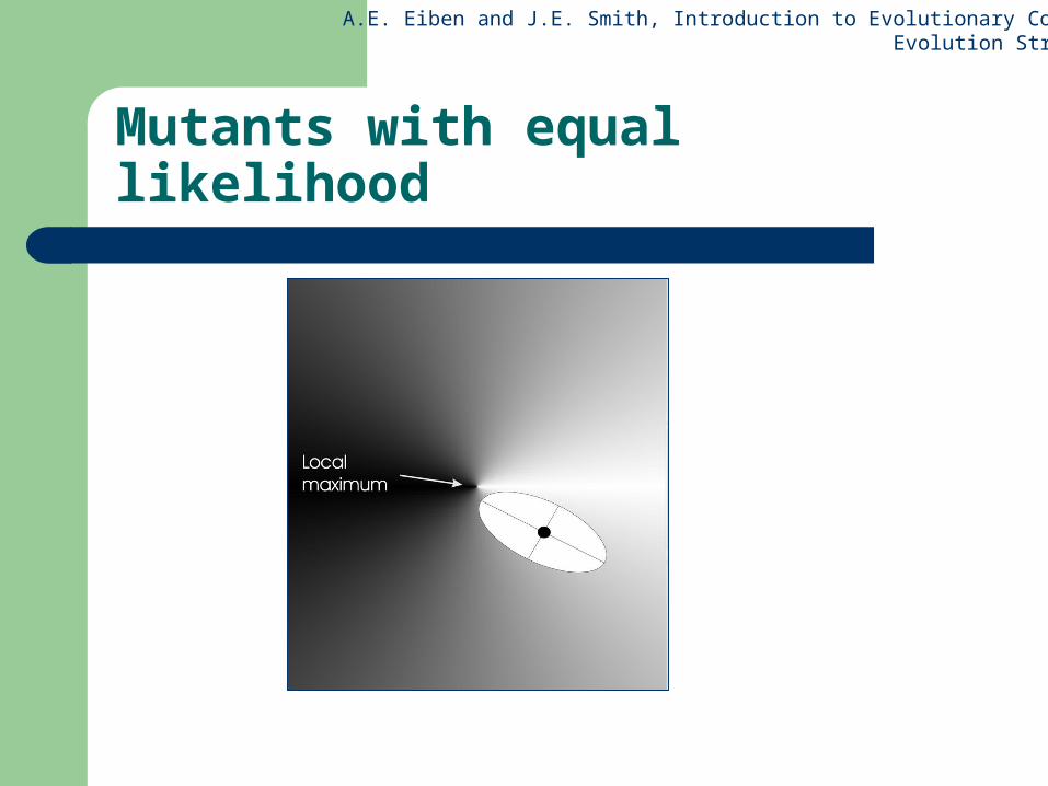
Mutation case 1:Uncorrelated mutation with one
Chromosomes: x1,…,xn, ’ = • exp( • N(0,1)) x’i = xi + ’ • N(0,1) Typically the “learning rate” 1/ sqrt(n) And we have a boundary rule ’ < 0 ’ = 0
A.E. Eiben and J.E. Smith, Introduction to Evolutionary ComputingEvolution Strategies
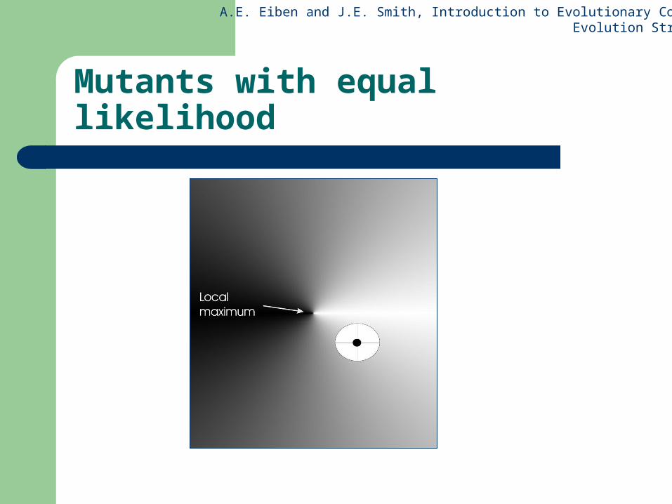
Mutants with equal likelihood
A.E. Eiben and J.E. Smith, Introduction to Evolutionary ComputingEvolution Strategies
Mutation case 2:Uncorrelated mutation with n ’s
Chromosomes: x1,…,xn, 1,…, n ’i = i • exp(’ • N(0,1) + • Ni (0,1)) x’i = xi + ’i • Ni (0,1) Two learning rate parmeters:
’ overall learning rate coordinate wise learning rate
1/(2 n)½ and 1/(2 n½) ½
And i’ < 0 i’ = 0
A.E. Eiben and J.E. Smith, Introduction to Evolutionary ComputingEvolution Strategies
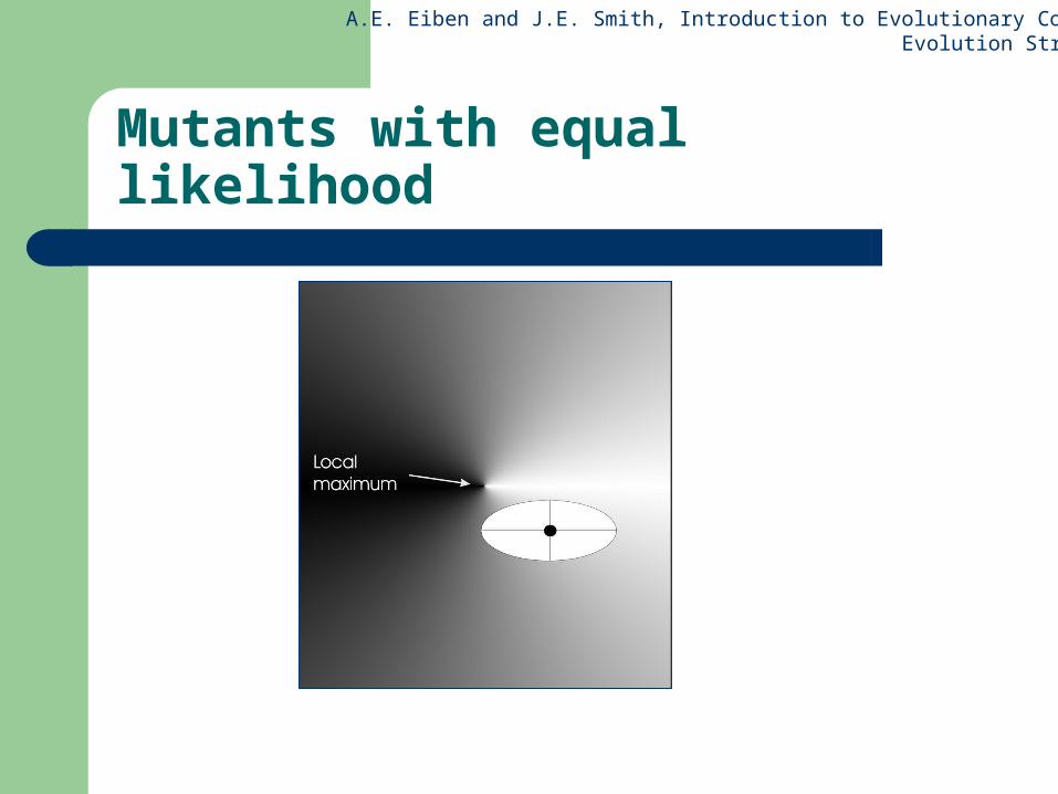
Mutants with equal likelihood
A.E. Eiben and J.E. Smith, Introduction to Evolutionary ComputingEvolution Strategies
Mutants with equal likelihood
A.E. Eiben and J.E. Smith, Introduction to Evolutionary ComputingEvolution Strategies
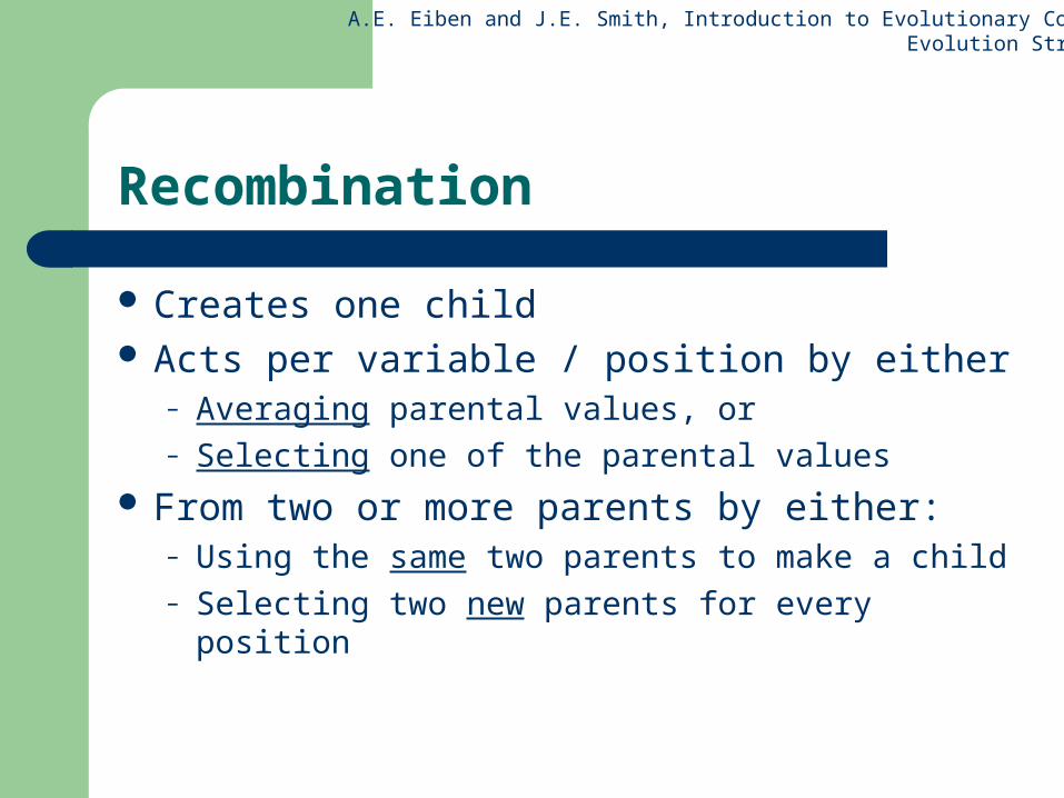
Recombination
Creates one child Acts per variable / position by either
– Averaging parental values, or– Selecting one of the parental values
From two or more parents by either:– Using the same two parents to make a child– Selecting two new parents for every position
A.E. Eiben and J.E. Smith, Introduction to Evolutionary ComputingEvolution Strategies
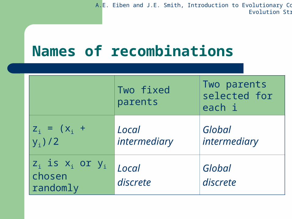
Names of recombinations
Two fixed parentsTwo parents selected for each i
zi = (xi + yi)/2 Local intermediary
Global intermediary
zi is xi or yi chosen randomly
Local
discrete
Global
discrete

A.E. Eiben and J.E. Smith, Introduction to Evolutionary ComputingEvolution Strategies
Parent selection
Parents are selected by uniform random distribution whenever an operator needs one/some
Thus: ES parent selection is unbiased - every individual has the same probability to be selected
Note that in ES “parent” means a population member (in GA’s: a population member selected to undergo variation)

A.E. Eiben and J.E. Smith, Introduction to Evolutionary ComputingEvolution Strategies
Survivor selection
Applied after creating children from the parents by mutation and recombination
Deterministically chops off the “bad stuff” Basis of selection is either:
– The set of children only: (,)-selection– The set of parents and children: (+)-selection

A.E. Eiben and J.E. Smith, Introduction to Evolutionary ComputingEvolution Strategies
Survivor selection cont’d
(+)-selection is an elitist strategy (,)-selection can “forget” Often (,)-selection is preferred for:
– Better in leaving local optima – Better in following moving optima– Using the + strategy bad values can survive in x, too long
if their host x is very fit
Selective pressure in ES is very high ( 7 • is the common setting)

A.E. Eiben and J.E. Smith, Introduction to Evolutionary ComputingEvolution Strategies
1. Initialize parent population
2. Generate offspring forming the offspring population where each offspring is generated by: – Select (uniformly randomly) parents
– Recombine the selected parents to form a recombinant individual – Mutate the strategy parameter set of the recombinant – Mutate the objective parameter set of the recombinant using the
mutated strategy parameter set to control the statistical properties of the object parameter mutation.
3. Select new parent population (using deterministic truncation selection) from either – the offspring population (this is referred to as comma-selection,
usually denoted as "-selection"), or – the offspring and parent population (this is referred to as plus-
selection, usually denoted as "-selection")
4. Go to 2. until termination criterion fulfilled.
A.E. Eiben and J.E. Smith, Introduction to Evolutionary ComputingEvolution Strategies
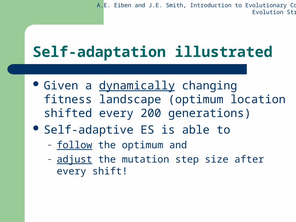
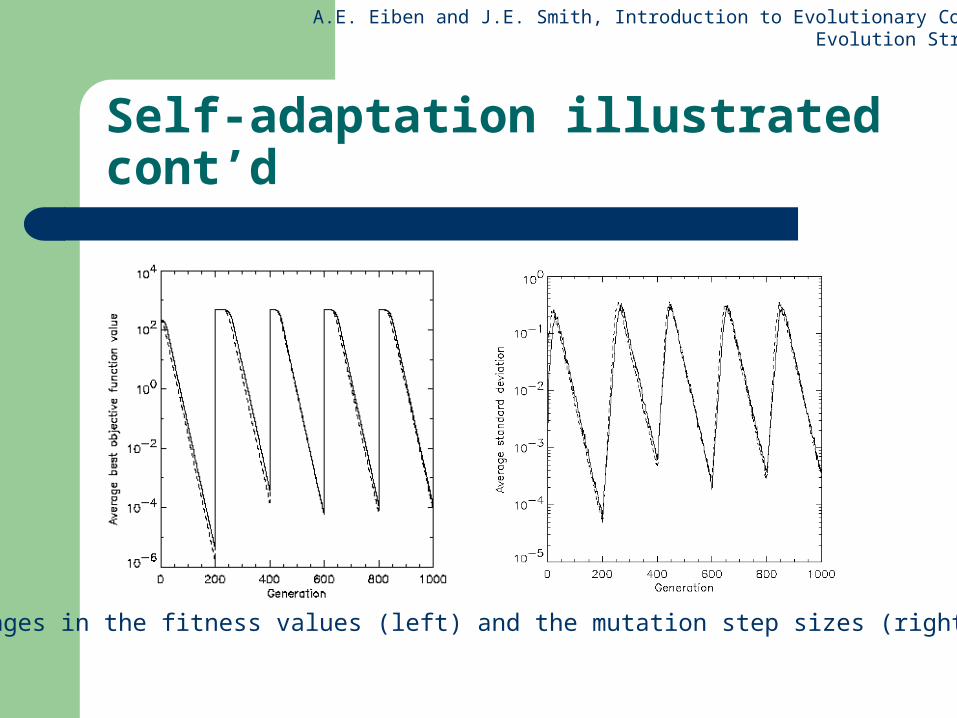
Self-adaptation illustrated
Given a dynamically changing fitness landscape (optimum location shifted every 200 generations)
Self-adaptive ES is able to – follow the optimum and – adjust the mutation step size after every shift!
A.E. Eiben and J.E. Smith, Introduction to Evolutionary ComputingEvolution Strategies
Self-adaptation illustrated cont’d
Changes in the fitness values (left) and the mutation step sizes (right)
A.E. Eiben and J.E. Smith, Introduction to Evolutionary ComputingEvolution Strategies
Prerequisites for self-adaptation
> 1 to carry different strategies > to generate offspring surplus Not “too” strong selection, e.g., 7 • (,)-selection to get rid of misadapted ‘s Mixing strategy parameters by (intermediary)
recombination on them

A.E. Eiben and J.E. Smith, Introduction to Evolutionary ComputingEvolution Strategies
Example application: the Ackley function (Bäck et al ’93)
The Ackley function (here used with n =30):
Evolution strategy:– Representation:
-30 < xi < 30 (coincidence of 30’s!) 30 step sizes
– (30,200) selection– Termination : after 200000 fitness evaluations– Results: average best solution is 7.48 • 10 –8 (very good)
exn
xn
xfn
ii
n
ii
20)2cos(1
exp1
2.0exp20)(11
2


![Ecologivcal Strategies in Fern Evolution[1]](https://static.fdocuments.in/doc/165x107/552729974a79594e118b464b/ecologivcal-strategies-in-fern-evolution1.jpg)