1. IntroductionThe Great Red Spot is an enduring large anticyclone in Jupiter's atmosphere, situated in the South Tropical Zone (Figure 1). Anticyclonic flow in this zone is perturbed over the northern edge of the GRS so that it locally protrudes into the typically dark and reddish South Equatorial Belt (SEB) to the north. The SEB features dramatic global-scale changes in coloration, cloud properties, and convective activity (e.g., Fletcher et al., 2011, 2017; Rogers, 1995; Sánchez-Lavega & Gómez, 1996), but the most notable change in the GRS itself is more monotonic in nature: a continuous decrease in size over more than 100 years of accurate ob-servations (Simon et al., 2018).

The size and longevity of the GRS make it unique among outer solar system vortices, yet it also serves as an archetype of a class of “pancake vortices”—anticyclones embedded in stably stratified fluids—also including vortices like the dark spots on Neptune and salt lens eddies in the Earth's oceans (e.g., Dowl-ing, 1995; Hassanzadeh et al., 2012; Yim et al., 2016). Pancake vortices have a thickness much smaller than their horizontal dimensions, like the GRS whose horizontal scale is some 50 times greater than vertical scale, according to theoretical arguments based on laboratory experiments and Jovian vortex velocity fields (Lemasquerier et al., 2020). Terrestrial ocean eddies transport heat meridionally by both stirring (turbulent) and trapping (bulk transport) mechanisms (Sun et al., 2018). Trapping is limited on Jupiter because major vortices are bounded by jets that limit meridional migration, although trapping could be significant on Saturn, where poleward migration of the anticyclone created by the 2,010 Great White Storm was observed

Abstract We measured the horizontal winds in Jupiter's Great Red Spot (GRS) using data from the WFC3/UVIS instrument on board the Hubble Space Telescope (HST). The data cover 11 epochs from 2009 to 2020. Long-term monotonic trends in size and shape previously noted from the visible cloud appearance are paralleled by changes in the high-speed ring around the vortex. The circularization of the GRS cannot be explained by changes in the horizontal wind shear of the surrounding environment. The velocity fields suggest no long-term trend in the static stability inside or outside the vortex. Instead, the changes are accompanied by a 4%–8% increase in the mean wind speeds of the high-speed ring from 2009 to 2020. Changes in the wind field coincided with the South Equatorial Belt Outbreak storms of 2016–2017, but not with 2019 "flaking" events involving detachment of red material from the main oval.

Plain Language Summary We measured the horizontal winds in Jupiter's Great Red Spot (GRS) using data from the WFC3/UVIS instrument on board the Hubble Space Telescope (HST). The data cover 11 time periods from 2009 to 2020. Winds blow fastest in a high-speed ring around the outside of the GRS. Previous pictures of the clouds showed that the GRS was shrinking and becoming more like a circle and less like an oval. We measure similar changes in the high-speed ring. We rule out some possible causes for the changes: changes in the wind shear of the surrounding atmosphere, or changes in how temperature varies with height. As the GRS shrinks and circularizes, the average wind speed in the high-speed ring gets faster. Some changes in the GRS wind patterns happened at the same time as a giant nearby storm in 2016/2017, but we did not find changes at the same time as flaking events in 2019. By "flaking" we mean pictures showing that small areas of red, normally kept inside the GRS, detached and blew away from the spot.

WONG ET AL.

© 2021 The Authors.This is an open access article under the terms of the Creative Commons Attribution-NonCommercial License, which permits use, distribution and reproduction in any medium, provided the original work is properly cited and is not used for commercial purposes.

Evolution of the Horizontal Winds in Jupiter's Great Red Spot From One Jovian Year of HST/WFC3 MapsMichael H. Wong1 , Philip S. Marcus1, Amy A. Simon2 , Imke de Pater1 , Joshua W. Tollefson1, and Xylar Asay-Davis3

1Center for Integrative Planetary Science, University of California, Berkeley, CA, USA, 2Solar System Exploration Division, NASA Goddard Space Flight Center, Greenbelt, MD, USA, 3Los Alamos National Laboratory, Los Alamos, NM, USA

Key Points:• A high-speed ring marking the edge

of the Great Red Spot velocity field has been shrinking and circularizing at a roughly constant rate

• Mean wind speeds within the high-speed ring have increased by 4%–8% from 2009 to 2020, at a roughly constant rate

• Velocity field changes coincided with a major 2016 storm, but we found no changes in 2019 when red material flaked away from the main oval

Supporting Information:Supporting Information may be found in the online version of this article.

Correspondence to:M. H. Wong,mikewong@astro.berkeley.edu

Citation:Wong, M. H., Marcus, P. S., Simon, A. A., de Pater, I., Tollefson, J. W., & Asay-Davis, X. (2021). Evolution of the horizontal winds in Jupiter's Great Red Spot from one Jovian year of HST/WFC3 maps. Geophysical Research Letters, 48, e2021GL093982. https://doi.org/10.1029/2021GL093982

Received 22 APR 2021Accepted 20 AUG 2021

10.1029/2021GL093982RESEARCH LETTER

1 of 10

Geophysical Research Letters

(Hueso et al., 2020; Sayanagi et al., 2013). Marcus (2004) suggested that the stirring mechanism—driven by the chaotic behavior of Jupiter's three white ovals near 34°S—would change after the ovals merged in 1997–2000, possibly leading to a temperature change at that latitude. The color change of merged Oval BA in 2006 might have resulted from a temperature change (e.g., de Pater et al., 2010; Wong et al., 2011), but the evidence is inconclusive in light of later changes in Oval BA back to white coloration (Simon, 2015), plus the general lack of high-resolution photometric time-series color information covering the white ovals in the decades prior to their mergers. Studying vortex evolution over time may allow comparison between planetary fluid environments from the atmospheres of the giant planets to the terrestrial oceans.

2. Data and MethodologyData were acquired by HST/WFC3 (Dressel, 2021) over the 2009–2020 time period by programs listed in Table S2. Additional 2014 data were not included because satellite-shadowing of the GRS region prevented high-precision velocity fields from being derived (Simon et al., 2014). Red wavelength (631–763 nm) filters optimize both spatial resolution and cloud tracer contrast. These “continuum” filters are sensitive to cloud opacity throughout the P < 10 bar region, but most of the clouds trace velocities at P < 1 bar in the GRS (Banfield et al., 1998). Image processing (Wong et al., 2020) consisted of correction for cosmic rays and de-tector distortion, and transformation from sky coordinates to Jovian latitude/longitude coordinates. We use planetographic latitudes and System III longitudes.

We retrieve the velocity field using the Advection Corrected Correlation Image Velocimetry technique (AC-CIV), which was specifically developed to measure velocities along curved paths in Jupiter's anticyclones (Asay-Davis et al., 2009; Asay-Davis, 2015). In a two-pass approach, we use data with a typical time separa-tion of 1.6 h for the initial pass, and 10.8 h for the final pass. At each iterative step, the velocity field from the previous iteration is used to advect the images to a common time point, and correlations are found between these advected images to refine the velocity field and to characterize the final uncertainties. We estimate an average “correlation velocity uncertainty” (Asay-Davis et al., 2009) of 3.6 ± 1.2 m s−1 among all the velocity fields (Table S4). The final output of ACCIV consists of one velocity field data set with the full set of scat-tered velocity vectors, and one sampled on a regular grid. Velocity fields and related data files are available in a public archive (Wong, 2021). The Supporting Information S1 discusses the error budget for uncertainty estimation, the archived data, and the ACCIV control parameters.

The overall dynamical structure of the GRS is defined by a ring of high-speed winds, which we use as a definition of the vortex dynamical boundary (even though the area just outside the high-speed ring is also part of the vortex; see Figure S3). Two alternate methods characterize the velocities in this ring:

WONG ET AL.

10.1029/2021GL093982

2 of 10

Figure 1. Jupiter data spanning one Jupiter year of HST/WFC3 observations, with zonal wind (blue) and Great Red Spot east-west (red) wind profiles overlaid. Arrows at right mark the latitude ranges of the South Equatorial Belt (SEB), South Tropical Zone (STrZ), and South Temperate Belt (STB). Color contrast has been maximized. Some subtle remaining color differences are due to different filter sets available at each epoch.

0 150 m/s–150 m/s 0 150 m/s–150 m/s 0 150 m/s–150 m/s

STrZSTB

SEB

2009.72R FQ634NG FQ437NB FQ378N

2019.48R F631NG F502NB F395N

2020.72R F631NG F502NB F343N

Geophysical Research Letters

1. We used an automated process to fit a symmetric ellipse to the data (see Supporting Information S1), thereby defining the vortex center location. Within the symmetric ellipse, we measured azimuthal ve-locities vellipse.

2. We defined a series of 100 “spokes” radiating from the center of the GRS with equal angular spacing, measuring the maximum azimuthal velocity vspokes along each spoke. The path connecting maxima along each spoke defines a lumpy ring, deviating from a perfect ellipse (Figure S2).

Figure 2 shows the 2020.72 velocity field, including the symmetric ellipse fit to the high-speed ring, gridded and scattered-vector velocity fields, the relative vorticity map, and cuts through the principal axes of the vor-tex. The global-average zonal wind field was subtracted to emphasize features of the velocity field specific to the vortex (except in Figure 2f).

3. ResultsThe relative vorticity map of the GRS, and the size and shape of the high-speed ring, are shown for each epoch in Figure 3. An outer region with a hollow core (Figure S3) can be seen at every epoch. The mean absolute value of the relative vorticity in the outer region remained in the 4 × 10−5 to 5 × 10−5 s−1 range throughout the timeline. Both the morphology and the unchanging constant relative vorticity are consistent with the study of Shetty and Marcus (2010), which found constant potential vorticity (a differ-ent quantity) within uncertainties, using a model of GRS velocity fields spanning 1979–2006. Constant relative vorticity implies constant potential vorticity only if static stability does not change over time, which we demonstrate below in the discussion of Figure 4c. Static stability can be expressed in terms such as the Brunt-Väisälä frequency, the deformation radius, or the lapse rate (e.g., Equation 1 of Wong et al., 2011).

Changes in the size of the vortex (Figure 4a and Table 1) extend the trends described in Simon et al. (2014, 2018). Extrapolating the linear decrease in size leads to an estimate that the GRS will reach a circular shape in 2035 based on HST/WFC3 data alone, or in 2039 if data extending back to Voyager are included.

Figure 4b shows that the mean wind speeds in the high-speed ring have increased over time. Weighted least squares fits give a rate of increase of 0.69 ± 0.25 m s−1 yr−1 using vellipse or 0.38 ± 0.25 m s−1 yr−1 using vspokes. Two separate statistical tests show that the increase is significant:

1. The Pearson's r values (Press et al., 1992, p.636), which are independent of measurement uncertainty, are r = 0.674 (with a false-alarm probability for linear correlation of 3.5%) for vellipse, and r = 0.579 (with a false-alarm probability for linear correlation of 8.2%) for vspokes.

2. Reduced χν2 values (which depend on measurement uncertainties) are 0.79 (for vellipse) or 0.77 (for

vspokes), with χν2 > 0.5 indicating that a linear slope is a good model for the variation (Bevington & Rob-

inson, 1992, p.197).

The spatial variability in values of vellipse or vspokes measured around the GRS circumference for a typical ve-locity field is shown by the shaded bars on the left side of Figure 4b, with magnitudes on the order of ±15 m s−1. The variability in velocities (also visible as lumps in the red ring in Figure 2b) is probably a real char-acteristic of the velocity field, rather than a result of errors in the retrieval process. We calculate χν

2 for the linear trend in Figure 4b, using the variability around the ring at each epoch (shaded bars) as an estimate of the mean speed uncertainty, rather than the error bars shown at each point based on the “correlation velocity uncertainty” described in Asay-Davis et al. (2009). The resulting χν

2 of 0.04 is unreasonably small, meaning that if the variability around the ring were truly due to measurement uncertainty (noise), then it is highly improbable that the data points would adhere so closely to the fitted lines shown.

Characteristics of the GRS flow field that are sensitive to the static stability (i.e., the vertical temperature profile) inside and outside of the vortex did not show strong trends (Figure 4c). To quantitatively constrain changes in the static stability (although we do not directly measure the static stability itself), we follow the work of Shetty et al. (2007), which found that the shape of east-west and north-south velocity profiles through the vortex center were sensitive to the potential vorticity. Potential vorticity is a nonlinear function of both the relative vorticity (velocity field gradient) and the static stability (expressed as the deformation radius LR in Shetty et al., 2007). Thus, if we could show that the relative vorticity in the GRS was unchanged,

WONG ET AL.

10.1029/2021GL093982

3 of 10

Geophysical Research Letters

and the shape of the velocity profile across the vortex was unchanged, we could conclude that the static stability in the vortex was unchanged. Figure  4c shows fluctuations of about ±25% in the GRS relative vorticity (gold points) and the decay factors characterizing the flow inside (blue points) and outside (pink points) of the high-speed ring, which are respectively sensitive to the potential vorticity inside and outside the ring. The overall trend in the mean speed is not reflected in these data.

To rule out the possibility that changes in the GRS velocity field were due to changes in the environment of the vortex, we measured the mean wind shear (applying a linear fit to the zonal wind profile) over the

WONG ET AL.

10.1029/2021GL093982

4 of 10

Figure 2. Great Red Spot velocity field data for the 2020.72 epoch, which is part of the OPAL program (Simon et al., 2015). The mean zonal wind field has been subtracted from the 2D velocity fields. (a) Color composite map, with a blue ring indicating the best-fit symmetric ellipse of high-speed velocities. (b) Wind speed, after subtraction of the mean zonal wind profile. (c) Velocity vectors (104 vectors drawn from the full set of 5.9 × 106 vectors). (d) Relative vorticity, showing the “hollow” core. (e) Northward velocities along an east-west profile through the center of the ellipse. Individual north-south vector components within ±0.25° of the east-west line are shown in light red, with the mean profile shown in blue. A parameterized fit to the profile is shown in light gray. (f) As panel E, for eastward velocities along a north-south profile through the center.

90 80 70 60

-35

-30

-25

-20

-15

-10

Plan

etog

raph

ic L

atitu

de (d

eg)

90 80 70 60West Longitude (deg, Sys III)

-35

-30

-25

-20

-15

-10

Plan

etog

raph

ic L

atitu

de (d

eg)

90 80 70 60

-35

-30

-25

-20

-15

-10

Plan

etog

raph

ic L

atitu

de (d

eg)

90 80 70 60West Longitude (deg, Sys III)

-35

-30

-25

-20

-15

-10

Plan

etog

raph

ic L

atitu

de (d

eg)200.0 m s–1

0

20

40

60

80

100

120

Velo

city

mag

nitu

de (m

/s)

-1�10-4

-5�10-5

0

5�10-5

1�10-4

Vorti

city

(s-1)

90 80 70 60West Longitude (deg, Sys III)

-150

-100

-50

0

50

100

150

Nor

th-s

outh

vel

ocity

(m s

-1)

-100 0 100Eastward velocity (m s-1)

-35

-30

-25

-20

-15

-10

Plan

etog

raph

ic L

atitu

de (d

eg)

A) Color mapHST WFC3 2020.72R F631NG F502NB F395N

C) Velocity vectors

E) Major axis profile

B) Velocity magnitude

D) Relative vorticity

F) Minor axis profile

Geophysical Research Letters

20–25°S range (Figure 4d). Methodology for the zonal wind retrievals is described in Asay-Davis et al. (2011) and Tollefson et al. (2017). There is no monotonic change in the wind shear (with the 2009 data point in-cluded) that parallels the long-term trends in vortex size, shape, and average wind velocity in the high-speed ring. Similarly, we found that the Rossby number of the GRS did not follow the long-term trends. The non-dimensional Rossby number Ro = U/fL characterizes the relative strength of inertial versus Coriolis forces, where U is the horizontal velocity scale, f is the Coriolis parameter, and L is the horizontal length scale.

The GRS Ro and the SEB wind shear did feature sudden changes in the 2016–2017 time period. The Rossby number increased from 0.105 ± 0.002 prior to 2016 to 0.127 ± 0.002 in 2016 and later, while there was a

WONG ET AL.

10.1029/2021GL093982

5 of 10

Figure 3. Relative vorticity maps (as in Figure 2d) for all epochs. At lower right, the evolution of the high-speed ring over the 2009–2020 period (shown at the same horizontal scale as the map panels) includes changes in shape and size on both short and long timescales.

260 250 240 230

-35

-30

-25

-20

-15

-10

Plan

etog

raph

ic L

atitu

de (d

eg)

240 230 220 210

-35

-30

-25

-20

-15

-10

140 130 120 110

-35

-30

-25

-20

-15

-10

260 250 240 230

-35

-30

-25

-20

-15

-10

Plan

etog

raph

ic L

atitu

de (d

eg)

0 -10 -20 -30

-35

-30

-25

-20

-15

-10

20 10 0 -10

-35

-30

-25

-20

-15

-10

40 30 20 10

-35

-30

-25

-20

-15

-10

Plan

etog

raph

ic L

atitu

de (d

eg)

160 150 140 130

-35

-30

-25

-20

-15

-10

280 270 260 250West Longitude (deg, Sys III)

-35

-30

-25

-20

-15

-10

300 290 280 270West Longitude (deg, Sys III)

-35

-30

-25

-20

-15

-10

Plan

etog

raph

ic L

atitu

de (d

eg)

90 80 70 60West Longitude (deg, Sys III)

-35

-30

-25

-20

-15

-10

-1�10-4

-5�10-5

0

5�10-5

1�10-4

Vorti

city

(s-1)

2012.722009.72

2017.25

2015.05

2018.29

2016.11

2019.27

2016.94

2019.48

2017.09

2020.72

2012.722009.72

2017.25

2015.05

2018.29

2016.11

2019.27

2016.94

2019.48

2017.09

2020.72 5000 km

Geophysical Research Letters

transient intensification of the SEB wind shear in 2017. The increase in the GRS Ro means that the flow of the vortex became slightly less “large scale” (i.e., less sensitive to planetary rotation, Pedlosky, 1987), but the vortex remains very much in the geostrophic regime.

WONG ET AL.

10.1029/2021GL093982

6 of 10

Figure 4. Evolution of the great red spot (GRS) velocity field. (a) There is a long-term decrease in size and aspect ratio of the high-speed ring, along with short-timescale variability. Data include previously published velocity fields from Voyager, Galileo, Cassini, and other HST instruments (Asay-Davis et al., 2009; Dowling & Ingersoll, 1988; Mitchell et al., 1981; Vasavada et al., 1998). (b) Two different methods produce a small but statistically significant increase in the mean wind speed in the high-speed ring of the GRS (see text). (c) Neither relative vorticity in the GRS outer region nor traits of the velocity field sensitive to atmospheric static stability showed long-term trends. Velocity field traits quantify the decay of wind speed inside (blue) and outside (pink) the high-speed ring as simple linear/exponential functions (thick gray line in Figure 2e). Data shown are averages of parameters for the east and west vertices of the GRS. (d) The STrZ windshear and the Rossby number characterizing the flow of the GRS high-speed ring both intensified around the time of the SEB Outbreak convective event in 2016/2017.

UT Date (series midpoint)Fractional

yearMajor width

(deg)Major width

(103 km)Minor width

(deg)Minor width

(103 km) Aspect ratioMean speed vellipse (m s−1)

Mean speed vspokes (m s−1)

2009-09-22 16:37 2009.72 13.27 ± 0.48 15.59 ± 0.56 9.05 ± 0.48 11.21 ± 0.60 1.39 ± 0.09 92 ± 14 103 ± 12

2012-09-20 15:42 2012.72 13.17 ± 0.66 15.44 ± 0.77 9.20 ± 0.74 11.40 ± 0.91 1.35 ± 0.13 89 ± 24 102 ± 17

2015-01-19 13:53 2015.05 12.99 ± 0.92 15.23 ± 1.08 8.80 ± 0.86 10.90 ± 1.07 1.40 ± 0.17 84 ± 19 97 ± 17

2016-02-09 16:03 2016.11 12.05 ± 0.76 14.17 ± 0.89 8.30 ± 0.72 10.28 ± 0.89 1.38 ± 0.15 92 ± 13 102 ± 11

2016-12-11 19:42 2016.94 11.11 ± 0.82 13.11 ± 0.97 7.20 ± 0.49 8.93 ± 0.61 1.47 ± 0.15 95 ± 18 100 ± 14

2017-02-01 22:50 2017.09 11.12 ± 0.84 13.02 ± 0.99 9.05 ± 0.76 11.21 ± 0.94 1.16 ± 0.13 97 ± 17 107 ± 16

2017-04-03 08:08 2017.25 11.77 ± 0.70 13.88 ± 0.83 8.25 ± 0.50 10.23 ± 0.62 1.36 ± 0.12 97 ± 13 105 ± 8

2018-04-17 07:49 2018.29 11.74 ± 0.51 13.82 ± 0.59 8.20 ± 0.43 10.16 ± 0.54 1.36 ± 0.09 95 ± 17 105 ± 15

2019-04-09 18:44 2019.27 10.43 ± 0.66 12.21 ± 0.78 8.50 ± 0.71 10.52 ± 0.88 1.16 ± 0.12 100 ± 12 108 ± 11

2019-06-26 12:46 2019.48 11.93 ± 1.02 13.96 ± 1.19 8.20 ± 0.81 10.15 ± 1.01 1.37 ± 0.18 96 ± 17 107 ± 11

2020-09-20 08:15 2020.72 10.59 ± 0.49 12.41 ± 0.57 9.10 ± 0.67 11.27 ± 0.83 1.10 ± 0.10 99 ± 12 106 ± 9

Table 1 Retrieved Velocity Field Parameters Pertaining to the High-Speed Ring Around the Great Red Spot

Geophysical Research Letters

4. DiscussionLong-term change in the aspect ratio could be explained if there were a decrease in the magnitude of the anticyclonic shear in the surrounding flow, because shear in the environment of vortices causes departures from circular shape (e.g., Marcus, 1990; Moore & Saffman, 1971). The environmental wind shear over the 2009–2020 timeframe did not weaken. It is unclear whether the wind shear is intensifying over time (which would elongate rather than circularize the GRS in the absence of any other influences), or whether it is varying in a more complex way.

The velocity fields also rule out a long-term variation in static stability, through comparison of relative vorticity in the GRS outer region with the shape of the velocity profile across the ring (represented by “decay factors”). Shetty et al. (2007) showed that the east-west cut through the vortex center had a simpler shape compared to the north-south cut, where interactions with the zonal jet. also affect the velocity pro-files. Although Galileo Probe measurements and theoretical analyses suggest static stability varies with height (Magalhães et al., 2002; Sugiyama et al., 2006; Wong, 2009), quasi-geostrophic models such as Shetty et al. (2007) treat it as vertically uniform. Likewise, velocity fields reveal the horizontal wind field only cover a limited altitude range compared to the full vertical extent of the vortex. Subject to these types of limita-tions, vortex models constrained by imaging and wind field data have been extensively used to estimate atmospheric static stability on Jupiter, with many finding a deformation radius of about 2,000 km (e.g., Brueshaber & Sayanagi, 2021; Brueshaber et al., 2019; Cho et al., 2001; Shetty & Marcus, 2010).

Wind speeds vary azimuthally by about ±15 m s−1 around the circumference of the high-speed ring. This variability may include a time-dependent component, as suggested by Choi et  al.  (2007) to explain tra-jectory curves that did not converge in their velocity field analysis of Galileo imager data. Velocity fields from spacecraft and HST observations of Jovian vortices also varied as a function of azimuthal position angle, with effects seen in the derived relative vorticity maps and profiles (e.g., Choi et al., 2010; Mitchell et al., 1981; Sánchez-Lavega et al., 2021). These variations could result from perturbations within the high-speed ring such as Rossby waves (Choi et al., 2007).

Evolutionary processes in terrestrial ocean eddies may help explain the changes in the GRS, despite key differences between Jovian and terrestrial vortices such as compressibility. Measurements of the evolution of a “meddy” in the Atlantic Ocean between 1984 and 1985 showed a decrease in size accompanied by a slight increase in peak velocity (Schultz Tokos & Rossby, 1991), which may be explained by a redistribu-tion of angular momentum after erosion of the vortex core (Sutyrin, 2020). “Flaking” events in mid-2019 (Sánchez-Lavega et al., 2021), in which regions of red material were seen to detach from the GRS and persist outside the oval itself for some time, were not associated with significant deviation from the long term evo-lutionary trends. So even if long term trends (in vortex size, shape, and peak windspeeds) are attributed to vortex erosion, we agree with the findings of Sánchez-Lavega et al. (2021) that the flakes did not represent an increase in erosive activity.

Although we lack theoretical insight into the cause of significant velocity field changes seen in 2016, it is no-table that a major convective event at nearby latitudes—the South Equatorial Belt Outbreak (SEBO)— be-gan in December 2016 and persisted into 2017 (Rogers, 2018; de Pater et al., 2019). The GRS Rossby number had already begun to increase in February 2016, indicating a several-month development timescale prior to the outbreak of convective activity on 29 December 2016. A previous SEBO event occurred in November 2010 (Fletcher et al., 2017), but there were no velocity field data to determine if that event also affected the global wind shear over 20–25°S or the GRS Ro.

On the other hand, the GRS velocity field seems to be insensitive to an interaction with a large triangu-lar (STrD) phenomenon in 2017–2018. The STrD feature originated near a large cyclonic vortex (Rogers et al., 2018), supporting ideas that STrDs are visible manifestations of stagnation points in the interacting flow field of jets and vortices (Marcus et al., 2008). Features like the 2019 GRS flakes also were produced near stagnation points (Marcus et  al.,  2019). Perhaps stagnation point interactions are able to produce conspicuous changes in cloud appearance, but do not perturb a large span of pressure levels (i.e., by chang-ing the stratification) and thus do not affect properties like the GRS Ro and the zonal wind shear.

WONG ET AL.

10.1029/2021GL093982

7 of 10

Geophysical Research Letters

Vortex oscillations—in both shape and location—were seen in Voyager Neptune imaging (Smith et al., 1989; Sromovsky et al., 1993, 2002), and oscillations provide a major constraint for dynamical models (LeBeau & Dowling, 1998; Hadland et al., 2020; Polvani et al., 1990). A triple-vortex system on Saturn oscillated in longitude (del Río-Gaztelurrutia et al., 2018), although long-lived single Saturnian vortices did not oscillate in Voyager observations (Sánchez-Lavega et  al.,  2000). The GRS has a well-known 90-day oscillation in longitudinal position (Trigo-Rodriguez et al., 2000), which was perturbed during the flaking events of 2019 (Sánchez-Lavega et al., 2021). Short timescale variations in the GRS size/shape (Figure 3, Table 1) could be due to periodic oscillations or transient changes, but future high-cadence datasets are needed to compare this dynamical aspect of anticyclones in outer planet atmospheres.

Data Availability StatementAll data from this project are available from a science-product repository at the MAST archive (Wong et al., 2020).

ReferencesAsay-Davis, X. S. (2015). Corrected Correlation Image Velocimetry (ACCIV). GitHub Code Repository. https://github.com/xylar/accivAsay-Davis, X. S., Marcus, P. S., Wong, M. H., & de Pater, I. (2009). Jupiter’s shrinking Great Red Spot and steady Oval BA: Velocity meas-

urements with the ‘Advection Corrected Correlation Image Velocimetry’ automated cloud-tracking method. Icarus, 203(1), 164–188. https://doi.org/10.1016/j.icarus.2009.05.001

Asay-Davis, X. S., Marcus, P. S., Wong, M. H., & de Pater, I. (2011). Changes in Jupiter’s zonal velocity between 1979 and 2008. Icarus, 211(2), 1215–1232. https://doi.org/10.1016/j.icarus.2010.11.018

Banfield, D., Gierasch, P. J., Bell, M., Ustinov, E., Ingersoll, A. P., Vasavada, A. R., et al. (1998). Jupiter's Cloud Structure from Galileo Im-aging Data. Icarus, 135(1), 230–250. https://doi.org/10.1006/icar.1998.5985

Bevington, P. R., & Robinson, D. K. (1992). Data reduction and error analysis for the physical sciences. McGraw-Hill.Brueshaber, S. R., & Sayanagi, K. M. (2021). Effects of forcing scale and intensity on the emergence and maintenance of polar vortices on

Saturn and Ice Giants. Icarus, 361, 114386. (18pp). https://doi.org/10.1016/j.icarus.2021.114386Brueshaber, S. R., Sayanagi, K. M., & Dowling, T. E. (2019). Dynamical regimes of giant planet polar vortices. Icarus, 323, 46–61. https://

doi.org/10.1016/j.icarus.2019.02.001Cho, J. Y.-K., de la Torre Juárez, M., Ingersoll, A. P., & Dritschel, D. G. (2001). A high-resolution, three-dimensional model of Jupiter's Great

Red Spot. Journal of Geophysical Research, 106(E3), 5099–5106. https://doi.org/10.1029/2000JE001287Choi, D. S., Banfield, D., Gierasch, P., & Showman, A. P. (2007). Velocity and vorticity measurements of Jupiter's Great Red Spot using

automated cloud feature tracking. Icarus, 188(1), 35–46. https://doi.org/10.1016/j.icarus.2006.10.037Choi, D. S., Showman, A. P., & Vasavada, A. R. (2010). The evolving flow of Jupiter’s White Ovals and adjacent cyclones. Icarus, 207(1),

359–372. https://doi.org/10.1016/j.icarus.2009.10.013de Pater, I., Sault, R. J., Moeckel, C., Moullet, A., Wong, M. H., Goullaud, C., et al. (2019). First ALMA millimeter-wavelength maps of

Jupiter, with a multiwavelength study of convection. The Astronomical Journal, 158(4), 139. https://doi.org/10.3847/1538-3881/ab3643de Pater, I., Wong, M. H., Marcus, P., Luszcz-Cook, S., Ádámkovics, M., Conrad, A., et al. (2010). Persistent rings in and around Jupiter's

anticyclones-Observations and theory. Icarus, 210(2), 742–762. https://doi.org/10.1016/j.icarus.2010.07.027del Río-Gaztelurrutia, T., Sánchez-Lavega, A., Antuñano, A., Legarreta, J., García-Melendo, E., Sayanagi, K. M., et  al. (2018). A plan-

etary-scale disturbance in a long living three vortex coupled system in Saturn's atmosphere. Icarus, 302, 499–513. https://doi.org/10.1016/j.icarus.2017.11.029

Dowling, T. E. (1995). Dynamics of Jovian atmospheres. Annual Review of Fluid Mechanics, 27, 293–334. https://doi.org/10.1146/annurev.fl.27.010195.001453

Dowling, T. E., & Ingersoll, A. P. (1988). Potential vorticity and layer thickness variations in the flow around Jupiter's Great Red Spot and White Oval BC. Journal of the Atmospheric Sciences, 45, 1380–1396. https://doi.org/10.1175/1520-0469(1988)045/1380:PVALTV/2.0.CO;2

Dressel, L. (2021). Wide Field Camera 3 Instrument Handbook, Version 13.0. Baltimore MD: STScI.Fletcher, L. N., Orton, G. S., Rogers, J. H., Giles, R. S., Payne, A. V., Irwin, P. G. J., & Vedovato, M. (2017). Moist convection and the 2010–

2011 revival of Jupiter's South Equatorial Belt. Icarus, 286, 94–117. https://doi.org/10.1016/j.icarus.2017.01.001Fletcher, L. N., Orton, G. S., Rogers, J. H., Simon-Miller, A. A., de Pater, I., Wong, M. H., et al. (2011). Jovian temperature and cloud var-

iability during the 2009-2010 fade of the South Equatorial Belt. Icarus, 213(2), 564–580. https://doi.org/10.1016/j.icarus.2011.03.007Hadland, N., Sankar, R., LeBeau, R. P., & Palotai, C. (2020). EPIC simulations of Neptune's dark spots using an active cloud microphysical

model. Monthly Notices of the Royal Astronomical Society, 496(4), 4760–4768. https://doi.org/10.1093/mnras/staa1799Hassanzadeh, P., Marcus, P. S., & Le Gal, P. (2012). The universal aspect ratio of vortices in rotating stratified flows: Theory and simulation.

Journal of Fluid Mechanics, 706, 46–57. https://doi.org/10.1017/jfm.2012.180Hueso, R., Sánchez-Lavega, A., Rojas, J. F., Simon, A. A., Barry, T., del Río-Gaztelurrutia, T., et al. (2020). Saturn atmospheric dynamics

one year after Cassini: Long-lived features and time variations in the drift of the Hexagon. Icarus, 336, 23. https://doi.org/10.1016/j.icarus.2019.113429

LeBeau, R. P., & Dowling, T. E. (1998). EPIC simulations of time-dependent, three-dimensional vortices with application to neptune's great dark spot. Icarus, 132(2), 239–265. https://doi.org/10.1006/icar.1998.5918

Lemasquerier, D., Facchini, G., Favier, B., & Le Bars, M. (2020). Remote determination of the shape of Jupiter’s vortices from laboratory experiments. Nature Physics, 16(6), 695–700. https://doi.org/10.1038/s41567-020-0833-9

Magalhães, J. A., Seiff, A., & Young, R. E. (2002). The stratification of Jupiter's troposphere at the Galileo probe entry site. Icarus, 158(2), 410–433. https://doi.org/10.1006/icar.2002.6891

WONG ET AL.

10.1029/2021GL093982

8 of 10

AcknowledgmentsThe analysis is based on observations from programs listed in Table S2, made with WFC3 on the NASA/ESA HST, obtained at the Space Telescope Science Institute (STScI), which is operat-ed by AURA under NASA contract NAS 5-26555, with support from all programs listed except 13067, and additional support from program 13631. We are grateful for the STScI approval to repeat failed 2020 observations for program 15929, without which GRS velocities would have been impossible to measure. We appreciate high-quality review comments from two anonymous reviewers, which caused a factor of three expansion of the Supporting In-formation S1 document.

Geophysical Research Letters

Marcus, P., Asay-Davis, X., Wong, M. H., de Pater, I., & Go, C. (2008). New observations and simulations of Jupiter's Great, Little and Oval Red Spots and Stagnation Points and Their Interactions. AAS/Division for Planetary Sciences Meeting Abstracts, 40. http://ui.adsabs.harvard.edu/abs/2008DPS....40.5303M

Marcus, P. S. (1990). Vortex dynamics in a shearing zonal flow. Journal of Fluid Mechanics, 215, 393–430. https://doi.org/10.1017/S0022112090002695

Marcus, P. S. (2004). Prediction of a global climate change on Jupiter. Nature, 428(6985), 828–831. https://doi.org/10.1038/nature02470Marcus, P. S., Hassanzadeh, P., Wong, M. H., De Pater, I., Barranco, J., Lee, D. C., & Zhang, A. S. (2019). On the shedding of Jupiter's Red

Flakes. AGU fall meeting abstracts 2019, Abstract P13B-3505. https://ui.adsabs.harvard.edu/abs/2019AGUFM.P13B3505MMitchell, J. L., Beebe, R. F., Ingersoll, A. P., & Garneau, G. W. (1981). Flow fields within Jupiter's Great Red Spot and White Oval BC. Jour-

nal of Geophysical Research, 86(A10), 8751–8757. https://doi.org/10.1029/JA086iA10p08751Moore, D. W., & Saffman, P. G. (1971). Structure of a Line Vortex in an Imposed Strain. In J. H. Olsen, A. Goldburg, & M. Rogers (Eds.),

Aircraft wake turbulence and its detection. Springer. https://doi.org/10.1007/978-1-4684-8346-8_20Pedlosky, J. (1987). Geophysical fluid dynamics (2nd edition). Springer-Verlag.Polvani, L. M., Wisdom, J., Dejong, E., & Ingersoll, A. P. (1990). Simple dynamical models of Neptune's great dark spot. Science, 249(4975),

1393–1398. https://doi.org/10.1126/science.249.4975.1393Press, W. H., Teukolsky, S. A., Vetterling, W. T., & Flannery, B. P. (1992). Numerical recipes in C. The art of scientific computing. Cambridge

University Press.Rogers, J., Eichstädt, G., Jacquesson, M., Hansen, C., Orton, G., Momary, T., et al. (2018). The new South Tropical Disturbance and its in-

teraction with the Great Red Spot. European Planetary Science Congress. Abstract EPSC2018-562. https://meetingorganizer.copernicus.org/EPSC2018/EPSC2018-562.pdf

Rogers, J. H. (1995). The giant planet Jupiter. Campbridge University Press.Rogers, J. H. (2018). Jupiter in 2016–17: Summary of the mid-SEB outbreak. British Astronomical Association, Jupiter Section Report 17.

https://britastro.org/node/8103Sánchez-Lavega, A., Anguiano-Arteaga, A., Iñurrigarro, P., Garcia-Melendo, E., Legarreta, J., Hueso, R., et al. (2021). Jupiter’s Great Red

Spot: Strong interactions with incoming anticyclones in 2019. Journal of Geophysical Research, 126(4), 2020JE006686. https://doi.org/10.1029/2020JE006686

Sánchez-Lavega, A., & Gómez, J. M. (1996). The South Equatorial Belt of Jupiter, I: Its life cycle. Icarus, 121(1), 1–17. https://doi.org/10.1006/icar.1996.0067

Sánchez-Lavega, A., Rojas, J. F., & Sada, P. V. (2000). Saturn's zonal winds at cloud level. Icarus, 147(2), 405–420. https://doi.org/10.1006/icar.2000.6449

Sayanagi, K. M., Dyudina, U. A., Ewald, S. P., Fischer, G., Ingersoll, A. P., Kurth, W. S., et al. (2013). Dynamics of Saturn’s great storm of 2010-2011 from Cassini ISS and RPWS. Icarus, 223(1), 460–478. https://doi.org/10.1016/j.icarus.2012.12.013

Schultz Tokos, K., & Rossby, T. (1991). Kinematics and Dynamics of a Mediterranean Salt Lens. Journal of Physical Oceanography, 21(6), 879–892. https://doi.org/10.1175/1520-0485(1991)021<0879:KADOAM>2.0.CO;2

Shetty, S., Asay-Davis, X. S., & Marcus, P. S. (2007). On the Interaction of Jupiter's great red spot and zonal jet streams. Journal of the At-mospheric Sciences, 64(12), 4432–4444. https://doi.org/10.1175/2007JAS2097.1

Shetty, S., & Marcus, P. S. (2010). Changes in Jupiter’s Great Red Spot (1979-2006) and Oval BA (2000-2006). Icarus, 210(1), 182–201. https://doi.org/10.1016/j.icarus.2010.06.026

Simon, A. A. (2015). Outer Planet Atmospheres Legacy (“OPAL”). Barbara A. Mikulski Archive for Space Telescopes. https://doi.org/10.17909/T9G593

Simon, A. A., Tabataba-Vakili, F., Cosentino, R., Beebe, R. F., Wong, M. H., & Orton, G. S. (2018). Historical and contemporary trends in the size, drift, and color of Jupiter's Great Red Spot. The Astronomical Journal, 155(4), 151. https://doi.org/10.3847/1538-3881/aaae01

Simon, A. A., Wong, M. H., & Orton, G. S. (2015). First results from the Hubble OPAL Program: Jupiter in 2015. The Astrophysical Journal, 812(1), 55. https://doi.org/10.1088/0004-637X/812/1/55

Simon, A. A., Wong, M. H., Rogers, J. H., Orton, G. S., de Pater, I., Asay-Davis, X., et al. (2014). Dramatic change in Jupiter's Great Red spot from spacecraft observations. The Astrophysical Journal, 797(2), L31. https://doi.org/10.1088/2041-8205/797/2/L31

Smith, B. A., Soderblom, L. A., Banfield, D., Barnet, C., Bailevsky, A. T., Beebe, R. F., et al. (1989). Voyager 2 at Neptune: Imaging science results. Science, 246(4936), 1422–1449. https://doi.org/10.1126/science.246.4936.1422

Sromovsky, L. A., Fry, P. M., & Baines, K. H. (2002). The unusual dynamics of Northern Dark Spots on Neptune. Icarus, 156(1), 16–36. https://doi.org/10.1006/icar.2001.6761

Sromovsky, L. A., Limaye, S. S., & Fry, P. M. (1993). Dynamics of Neptune's Major Cloud Features. Icarus, 105(1), 110–141. https://doi.org/10.1006/icar.1993.1114

Sugiyama, K.-I., Odaka, M., Kuramoto, K., & Hayashi, Y.-Y. (2006). Static stability of the Jovian atmospheres estimated from moist adiaba-tic profiles. Geophysical Research Letters, 33(3), L03201. https://doi.org/10.1029/2005GL024554

Sun, B., Liu, C., & Wang, F. (2018). Global meridional eddy heat transport inferred from Argo and altimetry observations. Scientific Reports, 9, 1345. https://doi.org/10.1038/s41598-018-38069-2

Sutyrin, G. G. (2020). How Baroclinic vortices intensify resulting from erosion of their cores and/or changing environment. Ocean Model-ling, 156, 101711. https://doi.org/10.1016/j.ocemod.2020.101711

Tollefson, J., Wong, M. H., Pater, I. de, Simon, A. A., Orton, G. S., Rogers, J. H., et al. (2017). Changes in Jupiter's zonal wind profile preced-ing and during the Juno mission. Icarus, 296, 163–178. https://doi.org/10.1016/j.icarus.2017.06.007

Trigo-Rodriguez, J. M., Sánchez-Lavega, A., Gómez, J. M., Lecacheux, J., Colas, F., & Miyazaki, I. (2000). The 90-day oscillations of Jupiter's Great Red Spot revisited. Planetary and Space Science, 48(4), 331–339. https://doi.org/10.1016/S0032-0633(00)00002-7

Vasavada, A. R., Ingersoll, A. P., Banfield, D., Bell, M., Gierasch, P. J., Belton, M. J. S., et al. (1998). Galileo imaging of Jupiter's atmosphere: The Great Red Spot, Equatorial Region, and White Ovals. Icarus, 135(1), 265–275. https://doi.org/10.1006/icar.1998.5984

Wong, M. H. (2009). Comment on “Transport of nonmethane hydrocarbons to Jupiter’s troposphere by descent of smog particles” by Don-ald M. Hunten [Icarus 194 (2008) 616 622]. Icarus, 199(1), 231–235. https://doi.org/10.1016/j.icarus.2008.08.017

Wong, M. H. (2021). Jupiter Great Red Spot Velocity Fields from HST/WFC3 (GRSWFC3). Barbara A. Mikulski Archive for Space Telescopes, Dataset. https://doi.org/10.17909/t9-jfs3-p240

Wong, M. H., de Pater, I., Asay-Davis, X., Marcus, P. S., & Go, C. Y. (2011). Vertical structure of Jupiter's Oval BA before and after it red-dened: What changed? Icarus, 215(1), 211–225. https://doi.org/10.1016/j.icarus.2011.06.032

Wong, M. H., Simon, A. A., Tollefson, J. W., de Pater, I., Barnett, M. N., Hsu, A. I., et al. (2020). High-resolution UV/Optical/IR Imaging of Jupiter in 2016-2019. The Astrophysical Journal Supplement Series, 247(2), 58. https://doi.org/10.3847/1538-4365/ab775f

WONG ET AL.

10.1029/2021GL093982

9 of 10

Geophysical Research Letters

Yim, E., Billant, P., & Ménesguen, C. (2016). Stability of an isolated pancake vortex in continuously stratified-rotating fluids. Journal of Fluid Mechanics, 801, 508–553. https://doi.org/10.1017/jfm.2016.402

References From the Supporting InformationIñurrigarro, P., Hueso, R., Legarreta, J., Sánchez-Lavega, A., Eichstädt, G., Rogers, J. H., et al. (2020). Observations and numerical model-

ling of a convective disturbance in a large-scale cyclone in Jupiter's South Temperate Belt. Icarus, 336, 113475. https://doi.org/10.1016/j.icarus.2019.113475

Karalidi, T., Apai, D., Schneider, G., Hanson, J. R., & Pasachoff, J. M. (2015). Aeolus: A Markov Chain Monte Carlo Code for Mapping Ultracool Atmospheres. An Application on Jupiter and Brown Dwarf HST Light Curves. The Astrophysical Journal, 814(1), 65. https://doi.org/10.1088/0004-637X/814/1/65

Li, C., Ingersoll, A., Klipfel, A., & Brettle, H. (2020). Modeling the stability of polygonal patterns of vortices at the poles of Jupiter as revealed by the Juno spacecraft. Proceedings of the National Academy of Sciences, 117(39), 24082–24087. https://doi.org/10.1073/pnas.2008440117

Orton, G. S., Tabataba-Vakili, F., Eichstädt, G., Rogers, J., Hansen, C. J., Momary, T. W., et al. (2020). A Survey of small-scale waves and wave-like phenomena in Jupiter's atmosphere detected by JunoCam. Journal of Geophysical Research: Planets, 125(7), e06369. https://doi.org/10.1029/2019JE006369

Showman, A. P. (2007). Numerical Simulations of forced shallow-water turbulence: Effects of moist convection on the large-scale circula-tion of Jupiter and Saturn. Journal of the Atmospheric Sciences, 64(9), 3132. https://doi.org/10.1175/JAS4007.1

Valcke, S., & Verron, J. (1997). Interactions of Baroclinic isolated vortices: The dominant effect of shielding. Journal of Physical Oceanog-raphy, 27(4), 524–541. https://doi.org/10.1175/1520-0485(1997)027<0524:IOBIVT>2.0.CO;2

Wong, M. H. (2020). Velocity Field of Jupiter's Great Red Spot in December 2016. Dryad, Dataset. https://doi.org/10.6078/D18Q4H

WONG ET AL.

10.1029/2021GL093982

10 of 10

1

Geophysical Research Letters

Supporting Information for

Evolution of the Horizontal Winds in Jupiter’s Great Red Spot from One Jovian Year of HST/WFC3 Maps

Michael H. Wong (UCB), Philip S. Marcus (UCB), Amy A. Simon (NASA GSFC), Imke de Pater (UCB), Joshua W. Tollefson (UCB), Xylar Asay-Davis (LANL)

Contents of this file Introduction Discussion of ACCIV parameters

Table S1 Catalog of all velocity fields and epochs

Table S2 Table S3

Figure S1 Parameter fitting methodology Figure S2 Figure S3 Table S4 Table S5 Uncertainty estimation

Movie S1 (caption) Catalog of data types included in the archive

Table S6 Table S7 Table S8

2

Introduction

This Supporting Information file provides more information on the parameters controlling ACCIV velocity field retrievals, an expanded description of the analysis methods used, and a catalog of the datasets available on the archive node as well as the individual elements contained in each of these datasets.

The main paper presents one velocity field per epoch of observation. For some epochs, the archive node includes multiple candidate velocity field datasets for a single epoch. These multiple attempts were made to address flaws in the final long time-separation velocity fields, such as bald spots or erroneously high velocities. Selection of the best final velocity field for a given image series involves subjective evaluation. We have selected the best dataset for each epoch for presentation in the main article, but we retain the less favored candidate velocity fields in the archive so that interested readers may independently assess the robustness of the methodology and results. Those wishing to use ACCIV on their own data may also find the additional candidate velocity fields to provide valuable comparisons.

Discussion of ACCIV parameters

The algorithms of the ACCIV code are fully described in Asay-Davis, et al. (2009). The GitHub repository containing the code (Asay-Davis 2015; https://github.com/xylar/acciv) also includes extensive documentation of the parameters used to control the velocity field retrievals. As input to ACCIV, we provided image data mapped to a cylindrical grid at a latitude/longitude resolution of 0.05° per map pixel. In most cases, three iterations were performed to measure the initial velocity field from short time-separation data. This initial velocity field was then used to correlate long time-separation data from consecutive Jupiter rotations.

We used a standard set of ACCIV parameters in most cases. The parameters with perhaps the largest effect on the results govern the correlation box size and spacing. Our default values for these parameters are shown in Table S1.

In some retrievals, parameters were modified slightly from the values in Table S1, additional passes were added, or other minor parameters not listed in the table were further varied. We mention some exceptions in the last column of Table S3, but all exceptions can be discovered in the full ACCIV parameter files as used in the actual code runs: a defaultParameters.ascii file containing common parameters for the

3

dataset, and a parameters.ascii file corresponding to each pass of the iterative process (Table S6). These parameter files include in-line comments helping to make the function of each parameter more transparent to human readers.

Table S1. Standard set of ACCIV parameters.

short time separations long time separations

pass1 pass2 pass3 pass1 pass2 pass3 pass4 pass5

box 60 50 30 80 60 50 40 40

range 15 7 5 40 20 10 5 5

stride 4 4 8 8 6 4 2 2

Catalog of all velocity fields and epochs

The GRS-WFC3 MAST archive node created for this project (Wong 2021; https://archive.stsci.edu/hlsp/grs-wfc3) contains velocity fields and associated input/output data for each dataset listed in Table S3. The appearance of the GRS and its surroundings at each epoch is shown in Fig. S1. For epochs with multiple candidate velocity fields, the candidates are distinguished by a label suffix ("Dataset label" in Table S3). Suffixes such as “d12” relate to the relative timing of the data used to construct velocity fields. Suffix d12 means the initial short time-separation velocity field was based on the first Jupiter rotation/day (d1), and the final long time-separation velocity field then included data from the second Jupiter rotation (d2). In most cases, a single short time-separation velocity field was used as input to the first long time-separation velocity field retrieval pass. The “long” suffix is an exception meaning that two separate short time-separation velocity fields were combined in the first pass of the long time-separation velocity field retrieval: the d1 short time-separation velocity field was used to advect the rotation 1 data to a common time, and the d2 short time-separation velocity field was used to advect the rotation 2 data to the same common time.

Some minor label inconsistencies exist, in that velocity fields from 2015 and 2020 are from the OPAL program, even though the labels do not end in the string “opal”. HST Program IDs corresponding to each epoch (Table S2) can be used to identify the actual source of each dataset.

4

Table S2. Summary of observational data used for GRS velocimetry. UT Date (series

midpoint) Fractional

year

Pairs short / longa

Max ∆t short / longa

(hours)

Geocentric distance

(AU) WFC3 filter

Program IDsb

Program PIs

2009-09-22 16:37 2009.72 3 / 2 1.34 / 9.60 4.24 FQ634N 11559 de Pater

2012-09-20 15:42 2012.72 5 / 12 1.59 / 9.94 4.73 F763M 13067 Schneider

2015-01-19 13:53 2015.05 6 / 11 1.59 / 19.10 4.39 F631N 13937 Simon

2016-02-09 16:03 2016.11 3 / 4 1.59 / 9.97 4.56 F631N 14334 Simon

2016-12-11 19:42 2016.94 3 / 9 1.59 / 12.09 5.86 F631N 14661 Wong

2017-02-01 22:50 2017.09 6 / 6 1.64 / 11.13 5.04 F631N 14661 Wong

2017-04-03 08:08 2017.25 3 / 6 1.59 / 11.80 4.46 F631N 14756 Simon

2018-04-17 07:49 2018.29 3 / 6 1.59 / 11.13 4.48 F631N 15262 Simon

2019-04-09 18:44 2019.27 1 / 2 1.39 / 11.16 4.82 F631N 14661,15159, 15665

Wong, de Pater

2019-06-26 12:46 2019.48 3 / 3 1.59 / 9.82 4.32 F631N 15502 Simon

2020-09-20 08:15 2020.72 4 / 4 1.97 / 11.57 4.71 F631N 15929 Simon

a Number of image pairs used for the initial short time-separation velocity field and the final long time-separation velocity field derived by the ACCIV method (Asay-Davis et al., 2009). Each image pair has a specific time separation. We list the maximum time separations for all the pairs used to derive each short and long time-separation velocity field.

b Raw and calibrated data from the MAST archive can be accessed using HST program IDs. Data from programs 13937, 14334, 14756, 15262, 15502, and 15929 were acquired as part of the Outer Planet Atmospheres Legacy (OPAL) program (Simon et al., 2015). Data from 11559 are described in Wong et al. (2011), data from 13067 are described in Karalidi et al. (2015), and data from 14661, 15159, and 15665 are described in Wong et al. (2020).

5

Table S3. List of all velocity fields available at the MAST archive node.

Fractional year Dataset label

Selected for paper Exceptions and candidate evaluation notes

2009.72 grs09 X Used 11 passes (5 is standard) to clear bald spots in long time-separation vel. field

2012.72 grs12 X

2015.05 grs15-p4 Vertex points closer to symmetric ellipse, only used 4

passes in long time-separation vel. field

grs15-p5 X Smoother vel. field, less streaky

2016.11 grs16opal-d12 X Bald spot at south vertex, good correspondence betw.

lumpy ring and symmetric ellipse, typical vel. histogram

grs16opal-d21 Low velocity at south vertex, x/y cuts have malformed peaks, large low-vel. shoulder on histogram

2016.94 grs16pj03 X Used stride=4 in short/pass3, 5px larger range in long passes 1-3

2017.09

grs17pj04-d12 East vertex anomalously far south

grs17pj04-d21 Bald spot near core in y-cut plot

grs17pj04-long X Lowest high-vel. shoulder in histogram

2017.25 grs17opal-long X

2018.29 grs18opal-d12 X Smoother ring defined by max(vspokes), smoother x-cut

grs18opal-d21 X Low-vel. lump within ring defined by max(vspokes), sharper histogram, smoother y-cut

2019.27 grs19pj19 X

2019.48 grs19opal-d12 X

grs19opal-d23 Bald spots in x/y cuts, ring defined by max(vspokes) falls too far inside symmetric ellipse

2020.72 grs20 X

6

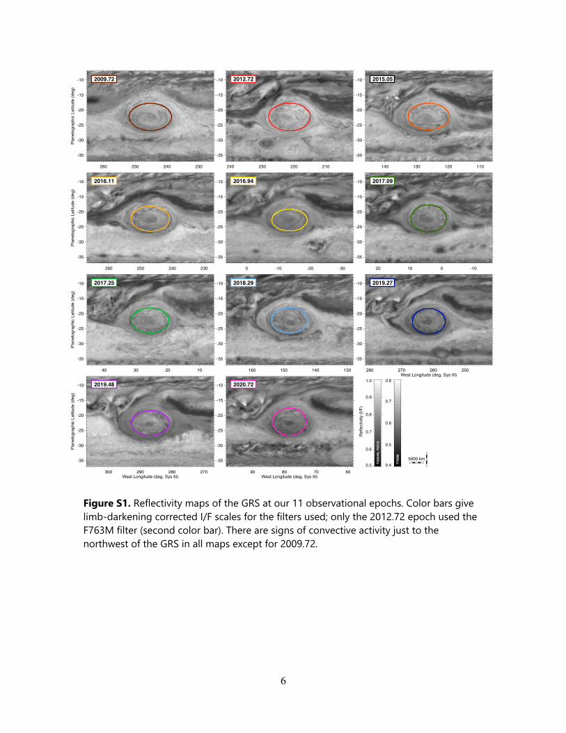
Figure S1. Reflectivity maps of the GRS at our 11 observational epochs. Color bars give limb-darkening corrected I/F scales for the filters used; only the 2012.72 epoch used the F763M filter (second color bar). There are signs of convective activity just to the northwest of the GRS in all maps except for 2009.72.

260 250 240 230

-35

-30

-25

-20

-15

-10Pl

anet

ogra

phic

Lat

itude

(deg

)

240 230 220 210

-35

-30

-25

-20

-15

-10

140 130 120 110

-35

-30

-25

-20

-15

-10

260 250 240 230

-35

-30

-25

-20

-15

-10

Plan

etog

raph

ic L

atitu

de (d

eg)

0 -10 -20 -30

-35

-30

-25

-20

-15

-10

20 10 0 -10

-35

-30

-25

-20

-15

-10

40 30 20 10

-35

-30

-25

-20

-15

-10

Plan

etog

raph

ic L

atitu

de (d

eg)

160 150 140 130

-35

-30

-25

-20

-15

-10

280 270 260 250West Longitude (deg, Sys III)

-35

-30

-25

-20

-15

-10

300 290 280 270West Longitude (deg, Sys III)

-35

-30

-25

-20

-15

-10

Plan

etog

raph

ic L

atitu

de (d

eg)

90 80 70 60West Longitude (deg, Sys III)

-35

-30

-25

-20

-15

-10

2012.722009.72

2017.25

2015.05

2018.29

2016.11

2019.27

2016.94

2019.48

2017.09

2020.72

0.5

0.6

0.7

0.8

0.9

1.0

Ref

lect

ivity

(I/F

)

0.4

0.5

0.6

0.7

0.8FQ

634N

, F63

1N

F763

M

5000 km

7

Parameter fitting methodology

Uniform processes were used to measure traits of each of the retrieved GRS velocity fields. Here we describe the detailed steps of the uniform processes.

A “sector fit” was the first step to locate the ellipse vertices. Human input was used to begin the process by graphically drawing a rectangle to fully enclose the high speed ring of the GRS, simplifying the procedure to find the GRS center within the velocity field domain. The user rectangle was divided into sectors. Each of the four sectors (north, west, south, and east) was defined in the radial direction as the half of the full user rectangle, bounded on one side by a line bisecting the center. Perpendicular to the radial direction, the sectors were bounded to the central 1/3 of that half of the rectangle. For example, the search sector for the northern vertex was defined by east-west segments at the top of the user rectangle and across the center of the rectangle, and by north-south segments located 1/3 of the east-west length of the user rectangle from its east and west limits. Within each search sector, the scattered (not the gridded) velocity vectors were divided into 25 groups with equal numbers of vectors, in the direction perpendicular to the radial direction for that sector (for example, 25 groups in the east-west direction for the north sector, whose radial direction is north). Each of these 25 groups was further divided into 51 bins in the radial direction (for example, the north-south direction for the north sector). The maximum velocity component in the direction perpendicular to the radial direction was then found and its location recorded for the 25 groups, defining a “sector trace” for each vertex.

The east and west vertex points from the sector fit were defined first, and most easily, because they rely on north-south velocities and are thus less affected by interactions between the vortex and its surroundings. These east-west vertex points were simply defined by the locations along the sector traces with the farthest radial distances from the initial vortex center approximated by the center of the user ellipse. Uncertainties in the positions of the east-west vertex points were estimated for latitudes as 1/2 the difference between the east and west point latitudes. For longitudes, uncertainties were estimated as the mean of two numbers: the longitude of the vertex point itself, and the longitude corresponding to the sector maximum north-south velocity at the latitude of the other vertex point. For example, for the east vertex point, the longitude uncertainty was estimated as the mean of the longitude of the east vertex point itself and the longitude along the eastern sector trace (a series of 25 points) corresponding to the latitude of the western vertex point.

The north and south vertex points from the sector fit were assigned to the longitude of the midpoint of the east and west sector vertex points. In fact, the center of the vortex is defined at this point as the mean of the east and west vertices from the sector fit. The latitudes for the north and south vertex points were taken as the median of latitudes along the sector trace, and latitude uncertainties were estimated as the standard deviation of latitudes along the sector trace.

8

Most of the quantities described above are available from the GRS-WFC3 MAST archive node in text and graphical form. For example, quantities related to the user-defined box enclosing the GRS are tabulated with keywords BOX_* (e.g., BOX_ELON for the longitude of the east edge of the box) in the *report.txt file for each velocity field, and the vertices from the sector fits are plotted as purple points with error bars in the *fit-map.pdf file for each velocity field (Table S8). Many of these parameters were output for validation and debugging purposes, and may not be of use to the majority of readers. Although we do not individually describe all ~140 parameters available in the *report.txt files here, the most useful parameters are listed in Table S3, and the lead author will provide additional description upon request from interested readers.

A symmetric ellipse was defined with semimajor diameter 2a = the distance between the sector fit east/west vertices, and semiminor diameter 2b = the distance between the north/south vertices. Figures 3 and S1 show the symmetric ellipse fits for each epoch. The center of the symmetric ellipse thus has the same longitude as the sector-fit center, but there is a latitude offset because the symmetric ellipse central latitude is defined using the north/south vertices, while the sector-fit central latitude is defined by the east/west vertices. Given prior analyses (e.g., Asay-Davis et al. 2009) describing the GRS velocity field in terms of an asymmetric ellipse (different values for b in the north and south directions), we used the sector-fit central latitude to define the GRS central latitude.

Coordinates and velocity data are listed in tabular form in the *report.txt files, for the symmetric ellipse fits, for the "lumpy" ring where vspokes data were obtained, and for the sector fits used to initially locate the vertices of the vortex. Spokes along which velocity maxima vspokes were found were separated by 3.6° azimuth for 100 evenly spaced spokes. Figure S2 shows an example of the lumpy vspokes ring for the 2020 data set. Equivalent data for the other velocity fields are available on the GRS-WFC3 MAST archive node.

Mean wind speeds in the high-speed ring: Wind speeds in Fig. 4B and Table 1 are average values around the entire circumference of the GRS. In Fig. 4B, we include average values from both vspokes and vellipse for two reasons: (1) they have different systematic errors due to the shape of the velocity field, and (2) even so, they both show the same overall increasing trend, so the trend is robust despite the systematic errors. By systematic errors, we mean that vspokes can sometimes mistakenly pick up fast vectors outside the high-speed ring, but it will never underestimate the speed in the ring. On the other hand, vellipse will never pick up fast vectors well outside the vortex, but it may miss fast vectors in the high speed ring when the shape of the fitted symmetric ellipse deviates from the actual shape of the vortex velocity field. In Tables S4 and S5, we show for comparison the maximum speeds in the cardinal directions near the vertices of the ellipse are listed. Trends are much more difficult to see in these tables, because real azimuthal variation in the wind speeds (see Figs. 2B and S2) contribute to the measurements.

9

Figure S2. LEFT: The symmetric ellipse (blue curve), lumpy ring of vspokes (green curve), and vertices from sector fit (purple points with error bars) are shown against a map of the GRS for the 2020.72 epoch. Similar maps are available on the GRS-WFC3 MAST archive node with filenames *fit-map.pdf inside the *_output-analysis.tar.gz bundle for all velocity fields. When purple error bars are not visible, the uncertainty estimates are smaller than the point. RIGHT: Velocities vspokes are shown as a function of azimuth, with both similarities and differences to the velocities along the symmetric ellipse. For example, the vspokes method jumped well outside the symmetric ellipse in the 20°-30° azimuth range (a green extension in the left panel, and a small sharp spike in the right panel). But the low speeds in vspokes (<100 m/s) at azimuth 225° is shared with velocities in the symmetric ellipse (see Fig. 2B). It is a real feature of the velocity field, rather than an artifact of the velocity field fitting method.

90 80 70 60West Longitude (deg, Sys III)

-35

-30

-25

-20

-15

-10

Plan

etog

raph

ic L

atitu

de (d

eg)

0 90 180 270 360Direction from GRS center (CCW from North)

80

90

100

110

120

130

140

Max

azi

mut

hal s

peed

(m/s

)

Mean valueUncertaintyMax individual vector

10

What is actually the dynamical boundary of the GRS? In this paper we use the high-speed ring to define a dynamical size/shape of the vortex and treat it as the dynamical boundary of the GRS, but other features of the velocity/vorticity fields could be chosen to represent the dynamical boundary, but we use the high-speed ring as the basis for the size/shape information shown in Fig. 4 and Table 1 of the main text. These contrast with the more familiar boundary from visible color (the red region). Another important aerosol/photometric boundary is defined by the upper tropospheric haze enhancement over the GRS.

In Fig. S3 we show regions of the GRS for the 2020 data. Just inside the high-speed ring is an outer region (dark purple) of nearly uniform relative vorticity (the basis for yellow points in Fig. 4C). Unlike smaller Jovian vortices, the GRS maintains a ”hollow core” (light purple) where relative vorticity is near zero (and may even be cyclonic; see Fig. 3 of the main text). Just outside the high-speed ring, winds decrease rapidly with radial distance from the GRS center, in a region of cyclonic shear (Valcke and Verron, 1997; Showman, 2007; Li et al., 2020; Brueshaber and Sayanagi, 2021). This outer cyclonic ring present at every epoch (Fig. 3), and should be considered part of the GRS itself. But its outer limit is difficult to quantitatively define, so the high-speed ring serves as a more useful dynamical boundary definition for comparing data at different epochs.

Blue absorption (Fig. S3D) is strongest near the hollow core region, but there appears to be a small offset from the location of the hollow core from the velocity field data. Haze opacity, from the methane-band data, closely matches the same morphology as the chromophore map (although areas outside the GRS show widespread differences between the haze and chromophore maps). The core/outer region are more distinct in the chromophore map, but more uniform in the haze map. This may be due to lower cloud opacity in the hollow core.

11

Figure S3. A: Important parts of the GRS include the outer anticyclonic region inside the high-speed ring, and a “hollow” core region with near-zero vorticity in the center. Outside of the high-speed ring, wind speeds decrease with radial distance (giving cyclonic shear). The ring of cyclonic shear is part of the GRS despite lying outside the high-speed ring we use as the dynamical boundary. B: The high-speed ring location is defined as described in the text; boundaries of the hollow core and the cyclonic shielding are drawn by hand based on the vorticity map shown in this panel. C: Color map shows the second Jupiter rotation (and thus differs from the first Jupiter rotation, shown in Fig. 2A). D: Blue absorption (i.e., chromophore distribution) is shown by the ratio of reflectivity (I/F) in the F658N and F395N filters. E: Composite map of three near-UV filters. F: Haze opacity from the methane-band map closely resembles the chromophore map, although the contrast between the core and outer region differs.

90 80 70 60

-35

-30

-25

-20

-15

-10

Plan

etog

raph

ic L

atitu

de (d

eg)

-20

Plan

etog

raph

ic L

atitu

de (d

eg)

90 80 70 60West Longitude (deg, Sys III)

-35

-30

-25

-20

-15

-10

Plan

etog

raph

ic L

atitu

de (d

eg)

90 80 70 60

-35

-30

-25

-20

-15

-10

90

90 80 70 60

-35

-30

-25

-15

-10

80 70 60West Longitude (deg, Sys III)

-35

-30

-25

-20

-15

-10

-1×10-4

-5×10-5

0

5×10-5

1×10-4

Vorti

city

(s–1

)

1

2

3

4

5

I/F

ratio

, 658

nm

/ 39

5 nm

0

0.05

0.10

0.15

0.20

I/F,

889

nm

C) Color mapHST WFC3 2020.72R F631NG F502NB F395N

E) Near ultraviolet mapHST WFC3 2020.72R F395NG F343NB F275W

D) Chromophores

A) Terminology

Cyclonic shielding

Outer region“Hollow” core region

B) Relative vorticity

F) Haze reflectivity

High-speed ring

12

Table S4. Additional velocity field characteristics.

Fractional year

Uncertainty (m/s) a Max. wind speed (m/s, along orthogonal axes) b

1-s Correl. North c West South East 2009.72 2.3 2.5 122.9 ± 1.8 104.4 ± 2.9 131.3 ± 3.5 109.5 ± 1.7

2012.72 2.9 3.7 131.5 ± 3.3 123.8 ± 3.6 156.5 ± 3.6 122.0 ± 3.5

2015.05 6.2 7.2 148.6 ± 2.0 112.7 ± 3.4 154.0 ± 11.5 111.4 ± 5.8

2016.11 2.6 3.4 131.0 ± 3.4 101.1 ± 1.2 169.9 ± 2.8 115.5 ± 2.8

2016.94 3.0 3.5 105.7 ± 1.7 109.1 ± 3.8 151.8 ± 3.1 113.5 ± 3.7

2017.09 2.8 3.3 145.1 ± 2.8 111.8 ± 4.2 166.7 ± 3.5 119.8 ± 3.9

2017.25 2.7 3.2 131.4 ± 2.4 105.4 ± 2.2 140.6 ± 3.6 113.1 ± 1.7

2018.29 2.5 3.0 161.5 ± 3.7 125.9 ± 3.1 138.1 ± 3.0 100.5 ± 2.3

2018.29 2.4 3.0 165.6 ± 2.7 116.0 ± 3.3 131.5 ± 3.2 103.0 ± 2.0

2019.27 2.9 3.3 145.8 ± 2.7 102.2 ± 2.0 162.6 ± 3.3 108.5 ± 3.1

2019.48 3.6 4.0 144.0 ± 4.2 129.7 ± 3.4 143.6 ± 3.3 114.1 ± 3.1

2020.72 3.0 3.4 144.7 ± 3.2 103.8 ± 2.8 153.2 ± 3.1 128.1 ± 2.7

a Uncertainties for each epoch are averaged over the full spatial domain of the velocity field. The first column gives 1-s uncertainties, which are the root-mean-square (RMS) averages of the deviations between the scattered velocity vectors in the final field and the velocity vector interpolated to that exact location from the gridded velocity field. This uses the inherent scatter in the velocity data to estimate uncertainty. The second column gives correlation velocity uncertainties, which are based on correlation displacements found using image data advected by the velocity field to a common time point. Both methods are described in greater detail in Asay-Davis et al. (2009), and in the next section of the Supplementary Information.

b Maximum wind speeds along the east-west and north-south cuts through the vortex center.

c Column heads give the location of the measurement with respect to vortex center. For example, in the 2009.72 velocity field, the maximum westward velocity to the north of the vortex center along the north-south minor axis was 122.9 m/s.

13

Table S5. Alternate measurement of maximum velocities in the cardinal directions.

Fractional year

Max. wind speed and position (m/s, degrees CCW from north) a

North b West South East 2009.72 145.2 336° 111.0 87° 111.0 167° 118.7 264°

2012.72 110.1 7° 148.2 78° 143.1 205° 131.4 271°

2015.05 147.6 330° 124.1 93° 135.9 186° 127.1 287°

2016.11 100.4 0° 109.0 101° 161.7 166° 122.1 269°

2016.94 83.1 337° 138.6 87° 126.0 185° 125.5 268°

2017.09 143.7 346° 124.5 93° 153.4 172° 129.2 265°

2017.25 126.4 339° 112.0 93° 121.7 186° 126.4 258°

2018.29 130.1 350° 135.5 93° 128.2 198° 114.7 255°

2018.29 139.1 2° 128.4 93° 122.1 207° 113.0 254°

2019.27 113.7 3° 107.5 85° 134.0 195° 116.7 278°

2019.48 124.0 11° 138.6 88° 113.6 174° 122.7 277°

2020.72 110.1 353° 113.3 86° 149.7 197° 136.7 265°

a Maximum wind speeds in the cardinal directions were found within the set of vspokes velocities (see right panel of Fig. S2).

b Column heads give the approximate location with respect to the vortex center, with azimuth measured in degrees counterclockwise from north. If the vortex were a perfect, uniform ellipse, the north, west, south, and east azimuth angles would be 0°, 90°, 180°, and 270°, but the data show that maximum values are often found off of the exact cardinal points. For example, in the 2009.72 velocity field, the maximum velocity in the westward direction was found along a spoke extending from the GRS center in the direction 336° east of north (i.e., 24° west of north or NNW), with a westward component of 145.2 m/s.

14

Uncertainty estimation

We follow a methodology for using dense velocity vector fields, and their associated source images, to self-consistently estimate the uncertainty in the final velocity field (see Section 3 of Asay-Davis et al. 2009, and the footnote for Table S4 above). For our GRS velocity fields, two separate estimates (the 1-s uncertainty and the correlation velocity uncertainty) give very similar results. We favor the estimate provided by the correlation velocity uncertainty (slightly larger than the 1-s uncertainty), which has an average value of 3.6 ± 1.2 m s–1 among all the final velocity fields in Table S4, or 3.3 ± 0.3 m s–1 when the 2015.05 dataset is omitted. For the short-time separation velocity fields (not listed in the tables), the correlation velocity uncertainty was 19.9 ± 3.3 m s–1 (omitting the 2015.05 dataset).

We suggest that the correlation velocity uncertainty represents an effective limit on the systematic precision of quantities derived from the final velocity fields, rather than a noise level that can be reduced by averaging together many velocity vectors. For example, consider the uncertainty in the mean speed within the high-speed ellipse, as shown by the blue error bars in Fig. 4B of the main text. These error bars show the standard deviation of velocity vectors near the high-speed ring (value MNELAZSG in the *report.txt files available on the archive), with MNELAZSG = 12–24 m s–1 depending on the individual dataset. The true uncertainty in the mean velocity over the high-speed ring should be (MNELAZSG2 + (correlation velocity uncertainty)2)0.5, but we have plotted MNELAZSG only in order to show the spatial variation over the ring. Thus the true uncertainty in the mean speed can never be lower than the correlation velocity uncertainty, which is the precision limit for the overall velocity field.

Systematic contributions to the velocity uncertainties include the limited resolution of the HST imaging data, the coherence/evolution of cloud tracer shapes over the duration of the time series used to measure velocities, and the curvature of paths traced by cloud tracking features. We address these systematic contributions here in response to concerns raised during peer review of this paper.

The spatial resolution of HST/WFC3 imaging data can be characterized in terms of the rectified pixel size of 0.0394 arcsec. We use this as a basis for estimating velocity uncertainty due to image resolution, although this simple number does not account for additional effects such as changes in the HST PSF (not Nyquist-sampled) due to breathing and shutter vibration, non-square pixel shape, target position angle, and resolution-dependent image navigation accuracy (typically smaller than a WFC3 pixel, see for example Wong et al. 2020, Inurrigarro et al. 2020). The corresponding velocity uncertainty due to limited spatial resolution is the 1-pixel size divided by the time separation. The 1-pixel size corresponds to an average of 132.7 km (see geocentric distances in Table S2), and our average time separations are 1.6 hours for the initial velocity fields and 10.8 hours for the final velocity fields (omitting the 2015 dataset, which included time separations up to 19.1 hours). The uncertainty due to spatial

15

resolution is thus about 23.2 m s–1 for short time separations, and 3.4 m s–1 for long time separations.

The spatial resolution error values are very close to the correlation velocity uncertainties, neglecting the 2015 case which is discussed separately below. This suggests that the ACCIV method is accurately estimating the uncertainties in the velocity field, because ACCIV actually does not know what the HST/WFC3 pixel size is. All of our maps are sampled at 0.05° latitude/longitude resolution, or about 57 km / map pixel (at the center of the GRS, 22°S). But the correlation velocity uncertainty is sensitive to the effective resolution of the images rather than the pixel or sampling resolution.

Cloud coherence timescales affect the time separations in image sequences that can be effectively used for velocity field measurements. Coherence timescales vary spatially. Our team has previously shown that cloud coherence timescales at HST spatial resolution are at least 10 hours for major anticyclones (Asay-Davis et al. 2009, Wong et al. 2011), but shorter than 10 hours for some features in the turbulent wake to the northwest of the GRS (Orton et al. 2020, Wong 2020).

The 2015.05 velocity field measurement included some unique aspects that validate our estimation of uncertainties, including the effects of image resolution and cloud coherence timescale.

Input maps to ACCIV for the 2015.05 observations were processed using an unsharp mask filter (radius 0.8° latitude/longitude). Figure S1 shows the original data, not the sharpened version used in ACCIV. All other epochs were not filtered to sharpen the map or image data. The resulting correlation velocity uncertainty for the short-timestep data in the 2015.05 dataset was 7.2 m s–1, much smaller than the average uncertainty of 19.9 ± 3.3 m s–1 for the unfiltered short-timestep datasets. It is not clear whether the filtering operation actually improves the accuracy of the short-timestep velocity fields. The unsharp mask filter takes information on larger spatial scales and concentrates it at shorter spatial scales, simulating an image at a higher effective resolution. However, the method is not capable of generating additional information about Jupiter’s clouds beyond what is contained in the original observation. We therefore suspect that the smaller correlation velocity uncertainty for the sharpened 2015 data corresponds to a more precise velocity field, but not one with improved accuracy.

Cloud coherence time was also tested in our 2015 dataset analysis by the inclusion of maps separated by about two Jupiter rotations (19.1 hours; Table S2). If cloud features remained perfectly coherent over this time separation, then the resulting uncertainty (based on spatial resolution divided by image time separation) should be close to 1.9 m s–1 (compared to 3.4 m s–1 for 10.8-hr separated data). Instead, the correlation uncertainty of 7.2 m s–1 for 19.1-hour separated data was more than twice as large as for the average 10.8-hr separated data (Table S4). We interpret the uncertainty values to mean that many cloud features at HST resolution are not coherent over ~20 hours. Thus,

16

velocity fields from data on a single Jupiter rotation are strongly limited by spatial resolution, velocity fields from data separated by two Jupiter rotations are limited by cloud coherence, and velocity fields from data separated by a single Jupiter rotation are ideal.

Streamline curvature becomes significant at the speed and length scales relevant to Jupiter’s large anticyclones, for data separated by one Jupiter rotation. The ACCIV method treats curved paths in two ways. First, the method works by iteratively improving the curved paths traced by cloud features. In Fig. 8 of Asay-Davis et al. (2009), errors in position are shown for correlated features advected forward and backward in time between an image pair. These displacement errors are used to estimate the uncertainty in the velocity field (the correlation velocity uncertainty), but they are also used to iteratively improve the velocity field by tracing a new curved trajectory that is interpolated between the original forward and backward paths. The second curvature treatment in ACCIV is that this new interpolated path is used to seed new velocity vectors (Fig. 29 of Asay-Davis et al. 2009) in the next iteration of the velocity field retrieval. Once the correlation velocity uncertainty stops decreasing with additional iterations, the method is considered to have converged on a velocity field.

Visual control and validation of the results can be conducted by viewing Movie S1. Errors in the velocity field would produce uncanny motion artifacts. Indeed, motion artifacts can be seen in the southeast area of Oval BA, but not in the GRS itself. The image maps were not optimized to measure velocities in Oval BA, which lies near the edge of the map domain, so the existence of velocity field errors there is not surprising. The velocity field errors produce motion artifacts seen as cloud features that exit to the southeast across the high-speed ring of Oval BA, then vanish and reappear in the northeast sector of the oval.

Movie S1. A movie simulating the flow in the GRS based on 2020 data is available just for fun on YouTube at https://youtu.be/G3_IcgHB1ik. It spans a duration of about 10 hours. In reality, the Great Red Spot would have rotated from day to night to day over this time period, so this movie would be impossible to record directly. The movie was created using the makeMovie.exe program included as part of the ACCIV distribution.

17

Catalog of data types included in the archive

On the GRS-WFC3 MAST archive node, each velocity field data set contains a collection of ACCIV input files, binary ACCIV output data, and summary/analysis output in image and text formats. Binary data are stored in HDF5 format. To facilitate working with the large number of individual files, we bundled related files into gzipped tarballs, with one bundle each for input data (Table S6), output velocity fields (Table S7), and output analysis plots and text files (Table S8). In a complete ACCIV run, a large number of intermediate output files is created. These intermediate files are not preserved on the archive node because we do not anticipate they will be useful to readers. The ACCIV parameter files and input map data files are sufficient to reconstruct all of these intermediate files if desired. In the main paper, Fig. 4 and Table 1 were constructed using the data stored in the *report.txt file for each epoch (Table S8).

Table S6. Catalog of input data files for each data set included at the MAST archive node. Files listed in this table are available from the *_inputs.tar.gz bundle for each epoch.

Element Filename/ extension File type input map grs*_nn.h5 HDF5 format, cylindrical map projection

ACCIV parameters *parameters.ascii Text format, ACCIV parameter files, one for each pass + one for each dataset

grid file grid*.h5 HDF5 format, grid files used to configure ACCIV recognition of map dimensions

Table S7. Catalog of output data files for each data set included at the MAST archive node. Files listed in this table are available from the *_output-data.tar.gz bundle for each epoch.

Element Filename/ extension File type

velocity vector file outScatteredVelocity.h5 HDF5 format, collection of velocity vectors from final long time-separation velocity field

velocity grid file outGridVelocity.h5 HDF5 format, gridded velocities from final long time-separation velocity field (derived from scattered vector field)

18

Table S8. Catalog of analysis output data files for each data set included at the MAST archive node. Files listed in this table are available from the *_output-analysis.tar.gz bundle for each epoch.

Element Filename/ extension File type

fit map *fit-map.pdf

PDF format, map showing GRS visible appearance, with overlays of the symmetrical ellipse location, the locus of maximum azimuthal velocities along radial spokes, and vertices of the vortex ellipse (ex., Fig. 2A in the main paper)

vector map *salvo.pdf PDF format, map showing a selection of 10,000 velocity vectors sampled from the scattered vector field, after subtraction of the zonal wind field (ex., Fig. 2C in the main paper)

velocity magnitude *vmag.pdf PDF format, map showing absolute magnitude of velocities from the gridded velocity field, after subtraction of the zonal wind field (ex., Fig. 2B in the main paper)

relative vorticity *RV.pdf PDF format, map showing relative vorticities calculated from the gridded velocity field after subtraction of the zonal wind field (ex., Fig. 2D in the main paper)

major axis profile *xcut.pdf PDF format, profile of north-south velocities along a cut through the vortex major axis including parameterized fit to the profile (ex., Fig. 2E in the main paper)

major axis profile *xcut.txt Text format, profile of north-south velocities along a cut through the vortex major axis (ex., pink curve in Fig. 2E in the main paper)

minor axis profile *ycut.pdf PDF format, profile of east-west velocities along a cut through the vortex minor axis (ex., Fig. 2F in the main paper)

minor axis profile *ycut.txt Text format, profile of east-west velocities along a cut through the vortex minor axis (ex., pink curve in Fig. 2F in the main paper)

azimuthal velocities *azi-ring.pdf PDF format, plot of the maximum azimuthal velocity along 100 spokes radiating from the vortex center, scatter in the measurements, and maximum individual velocity vector

azimuthal velocities *azi-ring.txt Text format, tabular information needed to recreate *azi-ring.pdf and the locus shown in *fit-map.pdf

velocity histogram *ring-histo.pdf PDF format, plot of velocity histogram within the envelope of the symmetrical ellipse

velocity histogram *ring-histo.txt Text format, tabular information needed to recreate *ring-histo.pdf

summary *report.txt Text format, list of GRS velocity field characteristics for each epoch/velocity field, including tabular data describing results from different fitting methods for characterizing the ring of high-speed velocities