Evolution of host plant selection in insects under...

Evolutionary Ecology Research, 2000, 2: 81–106

© 2000 Noél M.A. Holmgren

Evolution of host plant selection in insects underperceptual constraints: A simulation study

Noél M.A. Holmgren1* and Wayne M. Getz2

1Department of Natural Sciences, University of Skövde, Box 408, SE-541 28 Skövde, Sweden and2Department of Environmental Sciences, Management and Policy, University of California,

Berkeley, CA 94720-3112, USA

ABSTRACT

A major enigma in insect ecology is why many more host plant specialists than generalists exist,especially since laboratory and field experiments have indicated that specialists are usually ableto use a much broader spectrum of plants than is observed in nature. It has been suggestedthat perceptual constraints, coupled with considerations of foraging efficiency, may play a rolein the evolution of specialization. Here we investigate this notion in the context of insectsselecting different types of plants, where the ratios of particular compounds in a blend ofodorants provide the cues necessary to discriminate different plants from one another.The discrimination task is modelled by feedforward neural networks that are identified withparticular individuals. These networks replicate with the clonal reproduction of individuals,and the strength of the synapses in these networks are able to mutate from one generation to thenext. Individuals exploit the different plant types at a level determined by their perceptualresponse to the individual plants of each type. The fitness of individuals is determined by therelative nutritional value of each plant type and the proportion of individuals in the populationexploiting that plant type. From simulations of the evolution of the perceptual networks, we areable to conclude that the probability of particular preferences evolving depends on how closethe signals of the plants of different nutritive values are to one another. At reasonably highmutation rates, the more easily implemented plant preferences evolve earlier and are at a com-petitive advantage compared with later evolving, equally fit plant preferences. At low mutationrates, evolution stalls for long periods of time, but when change does occur it is saltational.Evolutionary equilibria typically involve guilds of complementary species that together consti-tute an ‘ideal free distribution’ in terms of the productivity of the different plants. Our resultsalso suggest: that the mix of phenotypes in these guilds is critically dependent on the orderof appearance of various combinations of specialist and generalist phenotypes; that thisorder depends on the difficulty of the perceptual task associated with each phenotype; thatany differences in the relative utilization by a generalist of different species of plants will lead tothe emergence of one or more specialists that exploit the plants most under-utilized by thegeneralist; and that evolutionary changes in guild structure are less frequent than mutationalrates might suggest, but are saltatory when they occur. Consequently, the strategy to specializemay dominate for two reasons: specialization appears to evolve more readily in complexenvironments; and the ideal free distribution mentioned above is more easily matched by agroup of specialists or by generalists in concert with specialists than by a generalist alone.Finally, our analysis suggests the hypothesis that oligophages or heterophages will not omit

* Author to whom all correspondence should be addressed. e-mail: [email protected]

Holmgren and Getz82

nutritive plants from their diet that have chemical signatures intermediate between plants uponwhich these herbivores feed.

Keywords: diet selection, evolutionary dynamics, feedforward networks, genetic algorithms,herbivory, niche selection.

INTRODUCTION

The concept of specialization can only be defined in a comparative sense (Futuyma andMoreno, 1988; Berenbaum, 1996). Herbivorous insects, for example, can be placed on aspecialist–generalist gradient by considering the number of species, genera or familiesof plants that they exploit (Jermy, 1984). However, specialist strategies are more commonthan generalist strategies (Jermy, 1984), which constitutes a major puzzle in entomologicalecology and evolution (Futuyma, 1991).

Several proposals have been made to explain selection for either specialists or generalists.The chemical defence theory states that specialization is required to overcome the chemicaldefences of a plant or group of plants (Swain, 1977). If a herbivore overcomes thesedefences, then colonization of these plants is facilitated (Feeny, 1987). Specialization hasalso been explained from a population ecological point of view. For example, predationmight select for specialists (Bernays and Graham, 1988) or specialization might evolve toenhance foraging performance (Bernays and Wcislo, 1994).

More recently, it has been suggested that specialization in insects may evolve due tolimitations in the perceptual system (Fox, 1993; Bernays and Wcislo, 1994; Janz and Nylin,1997; Bernays, 1998). In a complex environment, the information-processing capabilities ofan insect need to be focused on a limited number of identification tasks. Neurologicalcomplexity should allow increasingly sophisticated decision rules, and hence facilitate poly-phagy. In line with this idea, Levins and MacArthur (1969) suggested that insects areconstrained by their ability to discriminate among a number of suitable and unsuitable hostplants. We may therefore expect the underlying features of an insect sensory neural systemto be critical in determining the path taken by evolution towards particular species of insectherbivores becoming generalists or specialists.

Plant chemistry (taste and olfaction), rather than plant colour or shape (vision), isprobably the most fundamental factor in the process of individual herbivores acceptingor rejecting a plant (Bernays and Chapman, 1978). Some of these chemicals are volatileodours detectable at some distances, while non-volatiles (e.g. waxes) are detected by contactchemoreception or taste. Most olfactory receptors are located on the antennae (Visser,1986). They respond to an array of odorant molecules (Smith and Getz, 1994). Thisresponse is then propagated down the antennal nerve to the olfactory lobes in the insectdeutocerebrum (Masson and Mustaparta, 1990; Smith and Getz, 1994) where the infor-mation is processed and sent on to the higher levels of the brain (i.e. the mushroom bodiesin the protocerebrum; see Masson and Mustaparta, 1990; Hammer and Menzel, 1995).

Some structural features of insect olfactory systems may exist that correlate with thedegree of specialization across particular families of insects. Polyphagous species, forexample, appear to have more chemosensory sensilla than oligo- and monophagous species(Chapman, 1988). Orthopteran insects (grasshoppers and crickets) stand out as a groupdominated by polyphagous species (Bernays and Chapman, 1994). The brain of a typical

Evolution of host plant selection 83

orthopteran has about 1000 olfactory glomeruli in each of its two antennal lobes (Visser,1986). The brains of insects that have a more restricted diet (Bernays and Chapman, 1994)generally have fewer glomeruli (in some cases as few as 50; see Visser, 1986). Although otherfactors, such as the complexity of individual glomeruli, have some bearing on the com-plexity of chemosensory computations that individuals are able to perform, the chemo-sensory apparatus of polyphagous orthopterans suggests that they have evolved a morepowerful olfactory processing system than many other herbivorous insects that are lesspolyphagous. This suggests that polyphagy requires enhanced capabilities in memoryprocessing, as discussed by Dukas and Real (1991, 1993), and that neural structures associ-ated with memory and perception are energetically costly to maintain, or only evolve at theexpense of other adaptations.

Here we use artificial neural networks and population models to study the question ofperceptual constraints on the evolution of feeding behaviour in insects. Each individualinsect is represented by a simple network that processes plant chemosensory signals (Fox,1993). In these networks, synapse strengths are able to mutate during clonal reproduction(Enquist and Arak, 1994). The assumption of clonal reproduction implies that we do nothave to consider sexual recombination of genes coding for synapse strengths. This type ofassumption is often made in evolutionary analyses (Maynard Smith, 1982; Brown andVincent, 1987; Vincent and Brown, 1988), and the results are directly applicable to traitswith additive genetic variance under weak selection in sexually reproducing species (Taylor,1989; Kaitala and Getz, 1995; Getz, 1999; note that weak selection implies that pointmutations lead to small perturbations in traits). The network is capable of selectingamong plant types (i.e. resource niches), where the input to the networks is a signal thatis unique for each plant type and the output is a measure of the probability to utilizethat plant.

Futuyma, among others, has suggested that genetic constraints affect the evolutionarytrajectory of host preferences in insects (Futuyma, 1991; Futuyma, et al., 1993, 1995); but,to the best of our knowledge, this study represents the first attempt to investigate thesignificance of perceptual constraints on the evolution of host range in insects, using neuralnet models. Consequently, so as not to confound our results with other constrainingprocesses, we have kept the genetic coding, reproduction and fitness processes as simpleas possible. Thus, we focus here on how a class of neural networks (as detailed below),with their limitations and biases, will respond to selection in a number of different plantenvironments. We also investigate the effects of the frequency and the amplitude ofmutational changes.

THE MODEL

The model we use has three components: (1) computation of the perceptual response ofindividuals to different plant types, (2) calculation of the fitness of individuals, and (3)generation of progeny for the fittest individuals. The first component is modelled by asimple three-layer feedforward neural network (one sensory, one hidden and one outputlayer; Haykin, 1994). Each network represents an individual insect, and each plant typerepresents a resource capable of supporting the development and maturation of a fixednumber of individuals in each generation. The plants are assumed to produce a signal; thatis, the input to the neural network each individual uses to discriminate among plant types.The second component, the calculation of the fitness of each individual, is based upon

Holmgren and Getz84

(a) the response of its network to each of the plant types, (b) the productivity of thoseplant types, and (c) the number of individual competitors on those plants. The third com-ponent, reproduction of the fittest individuals, involves the replication and mutation of theassociated perceptual neural networks using algorithms detailed below.

Our model is particularly applicable to the evolution of guilds of holometabolous insectsthat lay their eggs on selected host plants. Our results, however, are equally applicable toother species for which the abstraction of processes embodied in our model provide a basicdynamical framework for their evolution. Our simulations are individual based (DeAngelisand Gross, 1992) and, because of random mutations, they are also stochastic. Therefore,simulations need to be repeated many times to obtain a sense of what the most likelyoutcomes will be over thousands of generations.

Odour perception and network model

Plants have a number of C6 compounds that, when mixed together, constitute what isgenerally known as ‘green odour’ (Visser, 1986; Olías et al., 1993). These universallycommon compounds occur in plant-specific ratios from which the plant species can berecognized (Bernays and Chapman, 1978; Visser and de Jong, 1987). A large number ofspecies have shown sensitivity to the components of green odour (Visser, 1986).

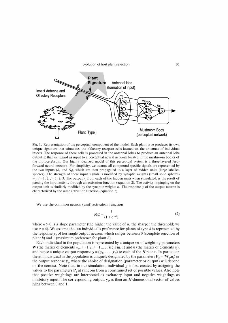
To keep our model simple, we assume that each type of plant is characterized by aspecies-specific ratio that is fed into the network via two input channels (S1 and S2), whereeach channel responds to the presence of plant compounds according to its own normalized‘tuning spectrum’ (cf. Getz and Akers, 1993). Note that limiting the inputs to two channelsdoes not imply that only two types of chemical are involved (e.g. see Dickinson et al., 1996).The input itself is preprocessed by afferent neurons to the location of this perceptualnetwork (Fig. 1). The most likely location for this perceptual network in insects is in themushroom bodies of the protocerebrum (for reviews, see Masson and Mustaparta, 1990;Smith and Getz, 1994). The olfactory input to the protocerebrum comes from the antennallobes, which in turn receive their input from sensory neurons located in the antenna (Fig. 1).For simplicity, we only consider the case where the perceptual network relies upon twoinputs from the antennal lobe. In actuality, this number is probably on the order of ahundred. Again, for simplicity, we ignore the complications of the effects of concentration(but see Masson and Mustaparta, 1990; Smith and Getz, 1994). In particular, we assumethat H plant types exist and that the signals from these H plant types produce characteristicresponses in the antennal lobes of individuals that are spaced out equidistant along the linejoining the points (S1, S2) = (0, 1) and (S1, S2) = (1, 0). That is, plants of type h produce theresponse

(S1,h,S2,h) = h

H + 1, 1 −

h

H + 1 where h = 1, . . .,H (1)

This response, generated in the projection neurons by the sensory neuron input into theantennal lobes, is then propagated to a fully connected, feedforward neural network (Fig. 1;see Haykin, 1994, for a didactic presentation of neural network theory). We select thenumber of hidden units to be one less than the number of plants, since this is the minimumnumber generally required to separate all plants from one another; and we select the numberof output units to be one.


We use the common neuron (unit) activation function

φ(ξ) =1

(1 + e−αξ)(2)

where α > 0 is a slope parameter (the higher the value of α, the sharper the threshold; weuse α = 4). We assume that an individual’s preference for plants of type h is represented bythe response yh of her single output neuron, which ranges between 0 (complete rejection ofplant h) and 1 (maximum preference for plant h).

Each individual in the population is represented by a unique set of weighting parametersW (the matrix of elements wij, i = 1,2, j = 1 ... 3; see Fig. 1) and u (the matrix of elements uj),and hence a unique output response y = (y1, . . ., yH) to each of the H plants. In particular,the gth individual in the population is uniquely designated by the parameters Pg = (Wg,ug) orthe output response yg, where the choice of designation (parameter or output) will dependon the context. Note that, in our simulation, individual g is first created by assigning thevalues to the parameters Pg at random from a constrained set of possible values. Also notethat positive weightings are interpreted as excitatory input and negative weightings asinhibitory input. The corresponding output, yg, is then an H-dimensional vector of valueslying between 0 and 1.

Fig. 1. Representation of the perceptual component of the model. Each plant type produces its ownunique signature that stimulates the olfactory receptor cells located on the antennae of individualinsects. The response of these cells is processed in the antennal lobes to produce an antennal lobeoutput Si that we regard as input to a perceptual neural network located in the mushroom bodies ofthe protocerebrum. Our highly idealized model of this perceptual system is a three-layered feed-forward neural network. For simplicity, we assume all compound-specific signals are represented bythe two inputs (S1 and S2), which are then propagated to a layer of hidden units (large labelledspheres). The strength of these input signals is modified by synaptic weights (small solid spheres)wi,j, i = 1, 2, j = 1, 2, 3. The output xj from each of the hidden units when stimulated, is the result ofpassing the input activity through an activation function (equation 2). The activity impinging on theoutput unit is similarly modified by the synaptic weights uj. The response y of the output neuron ischaracterized by the same activation function (equation 2).

Holmgren and Getz86

Finally, for clarification, we reiterate that the signal from each plant, after being pro-cessed at the level of the peripheral and antennal lobes of the insect brain, is assumed tobe invariant across individuals and to be constant throughout both the lifetime of theindividuals and through evolutionary time. In reality, however, this signal will show somevariation across individuals and, as with the network itself, will be affected to some degreeby experience and learning (Hammer and Menzel, 1995). Furthermore, in reality, we shouldexpect: variations in the signals across individual plants of the same type; the signals them-selves to evolve over time (actually co-evolve with the insect population); and, as previouslymentioned, the dimension of the signal to be higher than two (hundreds of relay neuronsproject from the antennal lobe to the mushroom body and, at least, tens of neurons shouldbe responding to any given stimulus at the periphery; see Laurent, 1996; Lemon and Getz,1999). As a first pass at analysing the evolution of specialization in plant choice usinga neural network approach, however, we ignore this level of detail and focus only on theevolution of choice as represented by the output response yg from the network modeldefined by the parameter set Pg that is fixed for the lifetime of an individual, but whichmutates from one generation to the next.

Ecological dynamics and fitness

The fitness of the individuals themselves is determined by their relative abilities to usethe plant signals to identify the most nutritious plants in an environment that has afinite carrying capacity (cf. the finite niche differential selection models of Levene, 1953;Dempster, 1955; Christiansen, 1975). The ecological dynamics and determination ofindividual fitness are based on the following idealizations:

1. Each individual has a total complement of E eggs.2. Individuals move around and lay their eggs in a number of clutches, with individual g

(g = 1, . . . ,G) ultimately laying cg,h of her eggs on plants of type h. All plant types areconsidered as hosts by every insect individual. The value of cg,h should reflect both therelative and absolute responses of individuals to plant type h; that is, cg,h depends bothupon

yg,hH

h = 1

yg,h

and upon yg,h itself. The latter implies that individuals who respond weakly to all plantswill end up laying only a small proportion of their egg complement E. From a modellingperspective, this assumption avoids a drift in absolute response values. From a biologicalperspective, it is reasonable to assume that a minimum response is required to stimulateegg laying in females.

3. The collection of all plants of type h represents a resource that produces a fixed numberrh of individuals whenever more than rh eggs are laid on that plant. This represents somehost-plant-related density-dependent effect that could be due to resource limitation,predation or any other limiting factor associated with the environment in question.

4. Every egg on a particular plant has the same probability to develop to maturity; that is,the probability of successfully completing the development cycle from egg to larva topupa to adult is independent of the individual phenotype Pg and all adults are equallyfecund.


Idealization (3) implies that density-dependence is infinitely abrupt (Getz, 1996), an ideal-ization that has been used elsewhere to study competition in evolutionary contexts (Levene,1953; Dempster, 1955; Christiansen, 1975; see also Getz and Kaitala, 1989). The simplestimplementation of idealization (2) is to use the expression

cg,h = yg,h

yg,h

H

h = 1

yg,h

E (3)

To demonstrate formula (3), suppose the environment has four types of plants (i.e. H = 4)and individual g has the same moderate response yg = (0.5, 0.5, 0.5, 0.5) to all plants. In thiscase, individual g will lay E/8 of its eggs in each of the four niches represented by these fourplant types; that is, it will lay only half of its egg complement E before it dies. On the otherhand, if individual g has the same strong response to all plants yg = (1,1,1,1), then it will layE/4 of its eggs in each of the four niches, thereby laying all of its egg complement E beforeit dies. Finally, if individual g responds only to plant type 2, but the response is maximal(i.e. yg = (0,1,0,0)), then this individual will lay all of her eggs only on plants of type 2.

Since each plant type is limited to producing rh individuals in the next generation,it follows from idealizations (1)–(4) that the expected number of offspring of individualg from niche h in the next generation is

rhcg,hG

g = 1

cg,h

so that its total number of offspring zg in the next generation is

zg = H

h = 1

rh

cg,h

G

g = 1

cg,h

(4)

Note that the fitness function represented by equation (4) does not explicitly or evenimplicitly favour a generalist selecting all suitable plants or a specialist selecting only oneplant. The fitness of an individual depends on the strategies of all other individuals throughthe competition that arises between the progeny of these individuals to get their pro-portional share of the resources in that niche.

Whatever the mutational processes are that drive the variation in the progeny of theindividual of phenotype Pg, and whatever the details are of the selection processes thattranslate the real number zg into an integer number of progeny, we should expect that at anevolutionary equilibrium the particular mix of phenotypes Pg, g = 1, . . . ,G, will representan ideal free distribution (i.e. each phenotype is equally fit; see Fretwell and Lucas, 1970;Parker, 1970). Furthermore, at the end of the evolutionary process (i.e. reaching a mix ofstrategies or drifting among equivalent mixes of strategies), this mix of strategies shouldrepresent a Nash equilibrium (Nash, 1951); that is, if the gth phenotype ‘tries’ alone tochange her ‘strategy’, represented by the values of the parameters Pg, then she can onlyreduce her fitness (see Lindgren, 1990, for similar results with regard to mixed strategies).

In all the simulations discussed below, we limit our investigation to an environmentwith four niches (i.e. H = 4) with a combined productivity of the 100 individuals – that is,

both ∑4

h = 1rh = 100 and G = 100.

Holmgren and Getz88

The evolution algorithm

The algorithm used to simulate the evolution of network phenotypes Pg is described by thefollowing six steps:

1. The first generation of individuals (reproductive adults) is created by initially selectingrandom values between 0.1 and −0.1 for the nine synaptic weights in Pg = (Wg,ug) foreach of the G = 100 phenotypes considered.

2. The output vectors yg and associated fitness values zg are then calculated using equations(1)–(4) for each of the 100 phenotypes Pg.

3. These fitness values zg, which are real numbers, are randomly rounded up or down asfollows: a rectangularly distributed random number between 0 and 1 is added to zg andthe result is then rounded down to obtain the number zg (i.e. all numbers of the form n.xwill be rounded up to n + 1 with probability 0.x and down to n with probability 1 − 0.x).

4. The 100 phenotypes are ranked in descending values of zg. The number of progenyassigned to each phenotype is zg. The total number of progeny should add up to anumber close to 100. If this number is more than 100, then the lowest ranking phenotypewith a single progeny will have its value zg reset from 1 to 0. This procedure will berepeated until the number of progeny is 100. Similarly, if the number of progeny is lowerthan 100, then the highest ranking phenotype with 0 progeny will have its value zg resetfrom 0 to 1. This will be repeated until the number of progeny is 100.

5. All the progeny inherit the synaptic weights of their mother, but each of these weightscan mutate as follows. Monte Carlo methods are used to determine which of the nineweights in Pg will be adjusted with probability π. Those to be adjusted have a randomvalue selected from a rectangular distribution centred on 0 and of width 2d (i.e. between−d and +d ) added to their current value. The procedure is continued until all 100 newprogeny have been assigned their mutated phenotype. These 100 progeny are then takento be the adult reproductives producing the next generation.

6. Steps 2–5 are repeated for T generations (we use T = 100,000).

Population index

The number of possible output phenotypes, yg, is essentially infinite, although we canround-off the values of elements yg,h in this vector to the nearest integer (i.e. 0 or 1) so thatwe obtain 2H categories of phenotypes. For purposes of discussion, we refer to phenotypesthat consist of all 0s or 1s with at least one 1 as ‘refined’, and all other phenotypes willbe referred to as ‘unrefined’. Because only the refined phenotypes lay their whole egg com-plement (see equation 3), evolution tends to produce only refined phenotypes. Thus therounding-off procedure allows us to classify all G individuals into 2H categories of refinedphenotypes and then plot the proportion of each category in the population. To reflect thefact that the unrefined phenotype yg = (0.75, 0.75, 0.25, 0.25), for example, is less like therefined phenotype yg = (1,1,0,0) than is the unrefined phenotype yg = (0.95, 0.95, 0.05,0.05), we use the following index Di, i = 1, . . . ,2H, to portray more accurately the proportion(multiplied by 100 to convert to a percentage) of individuals conforming to refined pheno-type category i (denoted by Ci):

Di =100

HG

g ∈Ci

H

h = 1

|2yg,h − 1| i = 1, . . . ,2H (5)


To illustrate how the index in expression (5) works, consider the unrefined phenotypeyg = (0.75, 0.75, 0.25, 0.25). Inserting these values in expression (5), we see that this pheno-type contributes 50/G to the index Di, while the refined phenotype yg = (1,1,0,0) contributes100/G. Additionally, the quantity

100 − ∑2H

i = 1Di

is a measure of how far evolution still has to go to produce refined phenotypes (the closerthis quantity is to 0, the more refined the phenotypes will be).

Types of runs

Simulations were run for the following six types of environments, Ωi, i = 1, . . .,6, eachbeing a vector of four rh elements: Ω1 = (50, 50, 0, 0) (i.e. niches 1 and 2 each produce 50individuals and niches 3 and 4 produce no individuals), Ω2 = (0, 50, 50, 0), Ω3 = (50, 0,50, 0), Ω4 = (40, 10, 40, 10), Ω5 = (30, 20, 30, 20) and Ω6 = (60, 0, 40, 0). EnvironmentsΩ1 = (50, 50, 0, 0), Ω2 = (0, 50, 50, 0) and Ω3 = (50, 0, 50, 0) represent an increasing orderof difficulty for the task of separating out the nutritious from the non-nutritious plants.We note from equation (1) that the ratio of the input signals S1,h/S2,h = h/(H + 1 − h)progressively increases from the first plant (h = 1: S1,h/S2,h = 1/H) to the last plant (h =H: S1,h/S2,h = H) as h increases from 1 to H. In particular, for H = 4, the four ratios inquestion are 1/4, 2/3, 3/2 and 4. To identify the nutritious plants in environment Ω1 asdistinct from the other plants requires that the network perform one discrimination task;for example, discriminate between ratios below and above 1. To identify the nutritiousplants in environment Ω2 as distinct from the other plants, however, requires that the net-work perform two discrimination tasks, for example, discriminate between ratios above andbelow 1/2 as well as ratios above and below 2. Thus, being a generalist in environment Ω1 isa more easily implemented discrimination task than being a generalist in environmentΩ2. Three discrimination tasks (discrimination levels) are required to be a generalist inenvironment Ω3.

For the six types of environments, we conducted simulations for the four cases obtainedfrom combinations of the probability-of-mutation parameter π = 0.02 or 0.1 (probabilitythat each synapse weight mutates) and mutation-range parameter d = 0.2 or 1.0 (therectangularly distributed half-range of the mutation). In each of the cases examined,simulations were repeated 100 times to obtain a sense of the average evolutionary trajectoryand its range of variation.

RESULTS

Arrangements of plants and the possibilities of categorization

One of the most striking features of our results is how the placement of the nutritious andnon-nutritious plants with respect to the response-induced input ratios, S1,h/S2,h, determineswhether specialist or generalists will evolve. As will become evident, this placement can bearranged in three qualitatively different ways (environments Ω1–Ω3).

Holmgren and Getz90

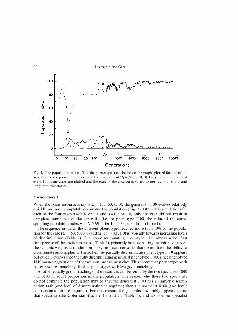
Environment 1

When the plant resource array is Ω1 = (50, 50, 0, 0), the generalist 1100 evolves relativelyquickly and soon completely dominates the population (Fig. 2). Of the 100 simulations foreach of the four cases π = 0.02 or 0.1 and d = 0.2 or 1.0, only one case did not result incomplete dominance of the generalist (i.e. for phenotype 1100, the value of the corre-sponding population index was Di ≥ 99) after 100,000 generations (Table 1).

The sequence in which the different phenotypes reached more than 10% of the popula-tion for the case Ω1 = (50, 50, 0, 0) and (π, d ) = (0.1, 1.0) is typically towards increasing levelsof discrimination (Table 2). The non-discriminating phenotype 1111 always arises first(irrespective of the environment; see Table 3), primarily because setting the initial values ofthe synaptic weights at random probably produces networks that do not have the ability todiscriminate among plants. Thereafter, the partially discriminating phenotype 1110 appearsbut quickly evolves into the fully discriminating generalist phenotype 1100, since phenotype1110 wastes eggs in one of the two non-producing niches. This shows that phenotypes withbetter resource-matching displace phenotypes with less good matching.

Another equally good matching of the resources can be found by the two specialists 1000and 0100 in equal proportion in the population. The reason why these two specialistsdo not dominate the population may be that the generalist 1100 has a simpler discrimi-nation task (one level of discrimination is required) than the specialist 0100 (two levelsof discrimination are required). For this reason, the generalist invariably appears beforethat specialist (the Order statistics are 1.8 and 7.3; Table 3), and also before specialist

Fig. 2. The population indices Di of the phenotypes (as labelled on the graph) plotted for one of thesimulations of a population evolving in the environment Ω1 = (50, 50, 0, 0). Only the values obtainedevery 10th generation are plotted and the scale of the abscissa is varied to portray both short- andlong-term trajectories.


Table 1. The final outcomes of the 100 simulations are listed for each of the four cases correspondingto two rates of mutation (π) and two ranges of deviation of the mutated weights (d ) and for each ofthe six environments Ωi considered*

Parameter settings

Environment and evolved phenotypesd =π =

1.00.1

1.00.02

0.20.1

0.20.02

1 = (50, 50, 0, 0)1100 (100)1000 (40) 0100 (40) 1100 (20)

991

100 100 100

2 = (0, 50, 50, 0)0110 (100)0100 0010 01100100 (50) 0010 (50)No Nash equilibrium

147961

1972

96

4

93

7

3 = (50, 0, 50, 0)1010 (100)1010 1000 00101000 (50) 0010 (50)No Nash equilibrium

2971

2899

581

1724

54

145

4 = (40, 10, 40, 10)1010 (60) 1111 (40)1000 0010 1010 1111 (40)1000 (30) 0010 (30) 1111 (40)1010 (40) 1110 (30) 1011 (30)1000 (20) 0010 (20) 1110 (30) 1011 (30)1000 (30) 0010 (20) 1110 (30) 0011 (20)No Nash equilibrium

18822

7

23

55311

35

49

14

46

15

85

5 = (30, 20, 30, 20)1010 (20) 1111 (80)1000 (10) 0010 (10) 1111 (80)1000 (10) 1110 (30) 0011 (20) 1111 (40)1110 (30) 1011 (30) 1111 (40)No Nash equilibrium

101323459

923

4343

3

394 100

6 = (60, 0, 40, 0)1000 (20) 1010 (80)1000 0010 10101000 (60) 0010 (40)No Nash equilibrium

35

902

11

8711

222

5521

5842

* In each row, immediately below the environments listed in the left column, the guild or combination of insectphenotype categories (Ci) obtained at the end of each 100,000 generation simulations is listed (the populationindices Di for each of the phenotypes are given in parentheses for the cases where the Nash equilibrium isobtained).

Tab

le 2

.T

he o

rder

of

phen

otyp

es r

each

ing

a po

pula

tion

ind

ex (

Di)

of

mor

e th

an 1

0% i

n th

e 10

0 si

mul

atio

ns o

f in

sect

s ad

apti

ng t

o ea

ch o

f si

xdi

ffer

ent

envi

ronm

ents

Ωi f

or t

he c

ase

(π, d

)=

(0.1

, 1.0

)

Ωi

50, 5

0, 0

, 0C

i

Nas

hC

ount

Ord

er

1111 100

1.0

1100 ** 100

2.0

1110 99 2.5

1000 *

100

3.6

0100 * 24 5.0

0, 5

0, 5

0, 0

Ci

Nas

hC

ount

Ord

er

1111 100

1.0

1110 71 2.2

0111 67 2.3

0110 ** 100

3.3

0100 ** 100

4.7

0010 ** 100

4.7

50, 0

, 50,

0C

i

Nas

hC

ount

Ord

er

1111 100

1.0

1110 99 2.4

1000 ** 100

2.6

0011 4

3.8

1010 * 20 3.9

0010 ** 99 4.1

40, 1

0, 4

0, 1

0C

i

Nas

hC

ount

Ord

er

1111 ** 100

1.0

1110 *

100

2.5

1000 ** 97 2.8

1010 * 24 3.8

1011 * 17 3.8

1001 1

4.0

0011 * 47 4.3

0010 ** 83 4.6

0111 2

5.0

0110 2

6.5

30, 2

0, 3

0, 2

0C

i

Nas

hC

ount

Ord

er

1111 ** 100

1.0

1110 ** 100

2.0

1011 ** 37 3.1

1010 * 10 3.1

0011 * 34 3.2

1000 * 35 3.9

0010 * 12 4.2

60, 0

, 40,

0C

i

Nas

hC

ount

Ord

er

1111 100

1.0

1100 2

2.0

1000 ** 100

2.1

1110 94 2.8

0011 8

3.1

0010 ** 100

4.1

1010 * 15 4.1

Not

e: T

he ta

ble

also

sho

ws

the

num

ber

of s

imul

atio

ns (c

ount

s) in

whi

ch th

e in

sect

phe

noty

pe c

ateg

orie

s (C

i) s

urpa

ssed

the

10%

leve

l, an

d th

e av

erag

e or

dina

l num

ber

inth

ese

sim

ulat

ions

. Phe

noty

pes

part

icip

atin

g in

Nas

h eq

uilib

rium

sol

utio

ns a

fter

100

,000

gen

erat

ions

are

indi

cate

d by

one

or

two

(for

the

mos

t co

mm

on)

aste

risk

s.

Tab

le 3

.T

he o

rder

of fi

rst a

ppea

ranc

e of

phe

noty

pes

(rea

chin

g a

popu

lati

on in

dex

(Di)

of m

ore

than

0.1

%) i

n th

e 10

0 si

mul

atio

ns o

f ins

ects

ada

ptin

gto

eac

h of

six

diff

eren

t en

viro

nmen

ts Ω

i for

the

cas

e (π

, d)

=(0

.1, 1

.0)

Ωi

50, 5

0, 0

, 0C

i

Nas

hC

ount

Ord

er

1111 100

1.0

0000 100

1.5

1110 100

1.7

1100 ** 100

1.8

0001 22 2.4

1000 *

100

2.5

0011 28 2.5

0111 34 2.6

0100 *

100

7.3

1101 94 7.5

1011 2

8.0

0110 36 8.5

1001 8

8.6

0010 0

1010 0

0101 0

0, 5

0, 5

0, 0

Ci

Nas

hC

ount

Ord

er

1111 100

1.0

0000 100

1.2

1110 100

2.5

0111 100

2.6

1100 100

4.2

0011 100

4.2

1000 56 4.9

0001 52 6.0

1001 4

6.8

1011 9

7.6

1101 1

8.0

0110 ** 100

8.3

0100 ** 100

9.1

0010 ** 100

9.2

1010 30

10.9

0101 25

11.2

50, 0

, 50,

0C

i

Nas

hC

ount

Ord

er

1111 100

1.0

0000 100

1.8

1110 100

2.0

1100 100

2.6

0111 84 3.6

1000 ** 100

4.2

0011 99 6.1

0001 46 6.5

0110 99 8.4

1101 9

8.4

0010 ** 100

8.7

1010 * 78

10.1

1011 46

10.3

1001 61

10.4

0100 22

12.0

0101

0

40, 1

0, 4

0, 1

0C

i

Nas

hC

ount

Ord

er

1111 ** 100

1.0

0000 100

1.5

1110 *

100

2.0

1100 100

3.2

0111 100

3.5

1000 ** 100

4.5

0011 * 98 5.0

0001 83 7.0

1101 36 9.4

1011 * 84 9.8

0110 95

10.0

1001 71

10.4

0010 ** 86

10.5

1010 * 56

10.7

0100 36

11.9

0101 0

30, 2

0, 3

0, 2

0C

i

Nas

hC

ount

Ord

er

1111 ** 100

1.0

0000 100

1.8

1110 ** 100

2.1

0111 100

2.9

1100 100

3.4

0011 *

100

4.7

1000 *

100

5.0

0001 91 6.8

1011 ** 97 9.1

1101 82 9.9

1001 78

10.7

0100 7

10.7

0110 77

10.8

1010 * 28

11.3

0010 * 48

11.5

0101 2

12.5

60, 0

, 40,

0C

i

Nas

hC

ount

Ord

er

1111 100

1.0

1110 100

1.6

0000 100

1.7

1100 100

2.4

1000 ** 100

3.2

0111 92 4.8

0001 61 6.1

0011 100

6.6

1101 12 7.2

0110 100

9.0

0010 ** 100

9.2

1001 66 9.8

1011 46

10.2

1010 * 73

10.4

0100 17

10.8

0101 0

Not

e: T

he ta

ble

also

sho

ws

the

num

ber

of s

imul

atio

ns (c

ount

s) in

whi

ch th

e in

sect

phe

noty

pe c

ateg

orie

s (C

i) s

urpa

ssed

the

0.1%

leve

l, an

d th

e av

erag

e or

dina

l num

ber

inth

ese

sim

ulat

ions

. Phe

noty

pes

part

icip

atin

g in

Nas

h eq

uilib

rium

sol

utio

ns a

fter

100

,000

gen

erat

ions

are

indi

cate

d by

one

or

two

(for

the

mos

t co

mm

on)

aste

risk

s.

Holmgren and Getz94

1000 (Order statistic 2.5). In addition, both specialists must appear virtually in the samegeneration if the combination of the specialist–generalist polymorphism is to be selectivelyneutral. Any specialist arising on its own will be selected against because the residentgeneralists will be more fit. Once the generalist – or, less likely, the pair of specialists – isestablished, the established phenotypes continue to dominate newly emerged phenotypesbecause the established phenotypes would be more refined in their category (i.e. the elem-ents in its response vector y are closer to 0s and 1s). Other factors aside, more refinedphenotypes are always more successful than less refined phenotypes.

Environment 2

The environment Ω2 = (0, 50, 50, 0) presents a more difficult discrimination task for thegeneralist 0110 (two levels of discrimination are required) than the environment Ω1 = (50,50, 0, 0) presents for the generalist 1100 (one level of discrimination is required). Further-more, in this environment, both specialists 0100 and 0010 require the same level ofdiscrimination as the generalist. Thus the specialists both arise on average at the same time,but later than the generalist (Tables 3 and 4). This is because fewer mutations are requiredfor the generalist than the specialist to evolve from the preceding phenotypes 1110 and0111 (see Table 2 for order of phenotypes appearing above the 10% population index level).

Interestingly, when the effects of the mutations are smaller (d = 0.2), specializationevolves much less frequently than when they are larger (d = 1.0; Table 1). In contrast tothe previous environment, the two specialists can evolve relatively easily from the alreadyexisting generalist. Provided the effects of the mutations are sufficiently large (d = 1.0),for most of the simulation the specialists 0100 and 0010 co-exist with the generalist0110 (Table 1 and Fig. 3). The proportion of specialists to generalists drifts, while the twospecialists themselves track each other. The reason for this is that the levels of competitionin the various niches are indifferent to replacing a pair of specialists 0100 and 0010 with twogeneralists 0110, but replacing any one of these three phenotypes with one of the othertwo upsets the competitive balance that maintains their co-existence.

The typical simulation in the case of environment Ω2 begins with the emergence ofunrefined forms of the phenotypes 0000 and 1111, where the latter dominates the popula-tion for a short period of time. Thereafter, phenotypes 0111 and 1110, which are able toreject one of the non-nutritive plants, spread in the population (Table 2). After runningthrough the gamut of one-level discriminator phenotypes, the two-level discriminatorphenotypes emerge and with them the Nash equilibrium polymorphism consisting of thegeneralist 0110 and specialists 0100 and 0010 evolves (Table 3).

Environment 3

The most difficult environment for the generalist phenotype to evolve in is Ω3 = (50, 0, 50,0), because the generalist phenotype 1010 must discriminate at three levels. Thus it isnot surprising in the two cases where d = 1.0 that the two specialists 1000 and 0010 evolveas Nash equilibrium solutions in 186 of the 200 simulations. First, they evolve earlier thanthe generalist (Table 3) and, secondly, the specialists are more resistant to mutations. Thesimpler the recognition task that a phenotype solves, the fewer the number of involvedsynaptic weights, and hence the lower the probability that a mutation will be deleterious.It is surprising, however, that the outcome with two specialists is only found in 18 of the

Tab

le 4

.T

he o

rder

of

phen

otyp

es r

each

ing

mor

e th

an 0

.1%

the

val

ue o

f th

e po

pula

tion

ind

ex (

Di)

in

the

100

sim

ulat

ions

of

inse

cts

adap

ting

to

envi

ronm

ent

Ω3 f

or t

he c

ase

(π, d

)=

(0.0

2, 0

.2)

Ωi

0, 5

0, 5

0, 0

Ci

Nas

hC

ount

Ord

er

1111 100

1.0

0000 98 1.0

1000 46 1.1

0001 40 1.3

1100 73 2.6

0011 73 3.0

0111 98 3.6

1110 97 3.7

0110 ** 84 6.9

0100 82 8.4

0010 78 8.5

1101 0

1011 0

1001 0

1010 0

0101 0

50, 0

, 50,

0C

i

Nas

hC

ount

Ord

er

1111 100

1.0

0000 100

1.0

0111 56 1.1

0001 40 1.3

0011 31 1.8

1110 100

2.9

1100 100

3.4

1000 * 69 3.7

1010 ** 42 6.6

0010 * 38 7.9

1011 29 8.9

0110 6

10.0

1101 0

0100 0

1001 0

0101 0

Not

e: T

he ta

ble

also

sho

ws

the

num

ber

of s

imul

atio

ns (c

ount

s) in

whi

ch th

e in

sect

phe

noty

pe c

ateg

orie

s (C

i) s

urpa

ssed

the

0.1%

leve

l, an

d th

e av

erag

e or

dina

l num

ber

inth

ese

sim

ulat

ions

. Phe

noty

pes

part

icip

atin

g in

Nas

h eq

uilib

rium

sol

utio

ns a

fter

100

,000

gen

erat

ions

are

indi

cate

d by

one

or

two

(for

the

mos

t co

mm

on)

aste

risk

s.

Holmgren and Getz96

200 simulations for the two cases where d = 0.2 (Table 1). The reason is that the generalistevolves before the second specialist (Table 4). As previously pointed out, if the two special-ists are to spread in the population, they have to evolve from the generalist more or lesssimultaneously.

In a typical run for the case (π, d ) = (0.1, 1.0) (Fig. 4), phenotype 1111 dominates forthe first 150 generations, after which phenotype 1110 and then specialist 1000 appear.Note, it is not before both specialists appear that the first specialist to emerge can increase,and that the two specialists together can outcompete the less fit generalist phenotype1110. Thus, for the case π = 0.02 and d = 0.1, the generalist 1010 evolves shortly after thelast specialist 0010, but the generalist soon disappears because it cannot compete withthe two specialists. These two specialist genotypes then persist for the remaining 10,000(Fig. 4) and 100,000 generations.

Reduced differences among niches

Although some plants may be very nutritious and others completely poisonous, manyplants will be of intermediate value to the insects that consume them. To investigate howplants of intermediate resource value affect the evolution of specialists and generalists, weexplored the evolution of choice in the two environments Ω4 = (40, 10, 40, 10) and Ω5 = (30,20, 30, 20). In these environments, one might expect generalists which distribute theirclutches across plants in direct proportion to the plants’ resource values (‘matchers’) to

Fig. 3. The population indices Di of the phenotypes (as labelled on the graph) plotted for one of thesimulations of a population evolving in the environment Ω1 = (0, 50, 50, 0). The values plotted are forevery generation up to 1000 generations, and thereafter every 100 generations. The scale of theabscissa is varied to portray both short- and long-term trajectories.


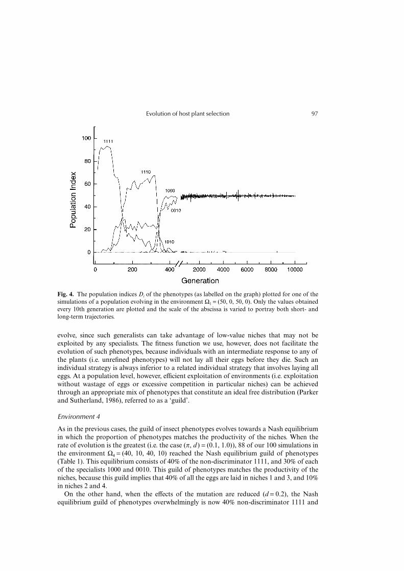
evolve, since such generalists can take advantage of low-value niches that may not beexploited by any specialists. The fitness function we use, however, does not facilitate theevolution of such phenotypes, because individuals with an intermediate response to any ofthe plants (i.e. unrefined phenotypes) will not lay all their eggs before they die. Such anindividual strategy is always inferior to a related individual strategy that involves laying alleggs. At a population level, however, efficient exploitation of environments (i.e. exploitationwithout wastage of eggs or excessive competition in particular niches) can be achievedthrough an appropriate mix of phenotypes that constitute an ideal free distribution (Parkerand Sutherland, 1986), referred to as a ‘guild’.

Environment 4

As in the previous cases, the guild of insect phenotypes evolves towards a Nash equilibriumin which the proportion of phenotypes matches the productivity of the niches. When therate of evolution is the greatest (i.e. the case (π, d ) = (0.1, 1.0)), 88 of our 100 simulations inthe environment Ω4 = (40, 10, 40, 10) reached the Nash equilibrium guild of phenotypes(Table 1). This equilibrium consists of 40% of the non-discriminator 1111, and 30% of eachof the specialists 1000 and 0010. This guild of phenotypes matches the productivity of theniches, because this guild implies that 40% of all the eggs are laid in niches 1 and 3, and 10%in niches 2 and 4.

On the other hand, when the effects of the mutation are reduced (d = 0.2), the Nashequilibrium guild of phenotypes overwhelmingly is now 40% non-discriminator 1111 and

Fig. 4. The population indices Di of the phenotypes (as labelled on the graph) plotted for one of thesimulations of a population evolving in the environment Ω1 = (50, 0, 50, 0). Only the values obtainedevery 10th generation are plotted and the scale of the abscissa is varied to portray both short- andlong-term trajectories.

Holmgren and Getz98

60% generalist 1010. Both this and the previous (π = 1.0) result are in accordance with theresults obtained for environment Ω3 = (50, 0, 50, 0), in the sense that the polyphagousphenotype 1111 is associated with both specialists 1000 and 0010 when the effects of themutations are relatively large and with the generalist 1010 when the effects of the mutationsare five times smaller.

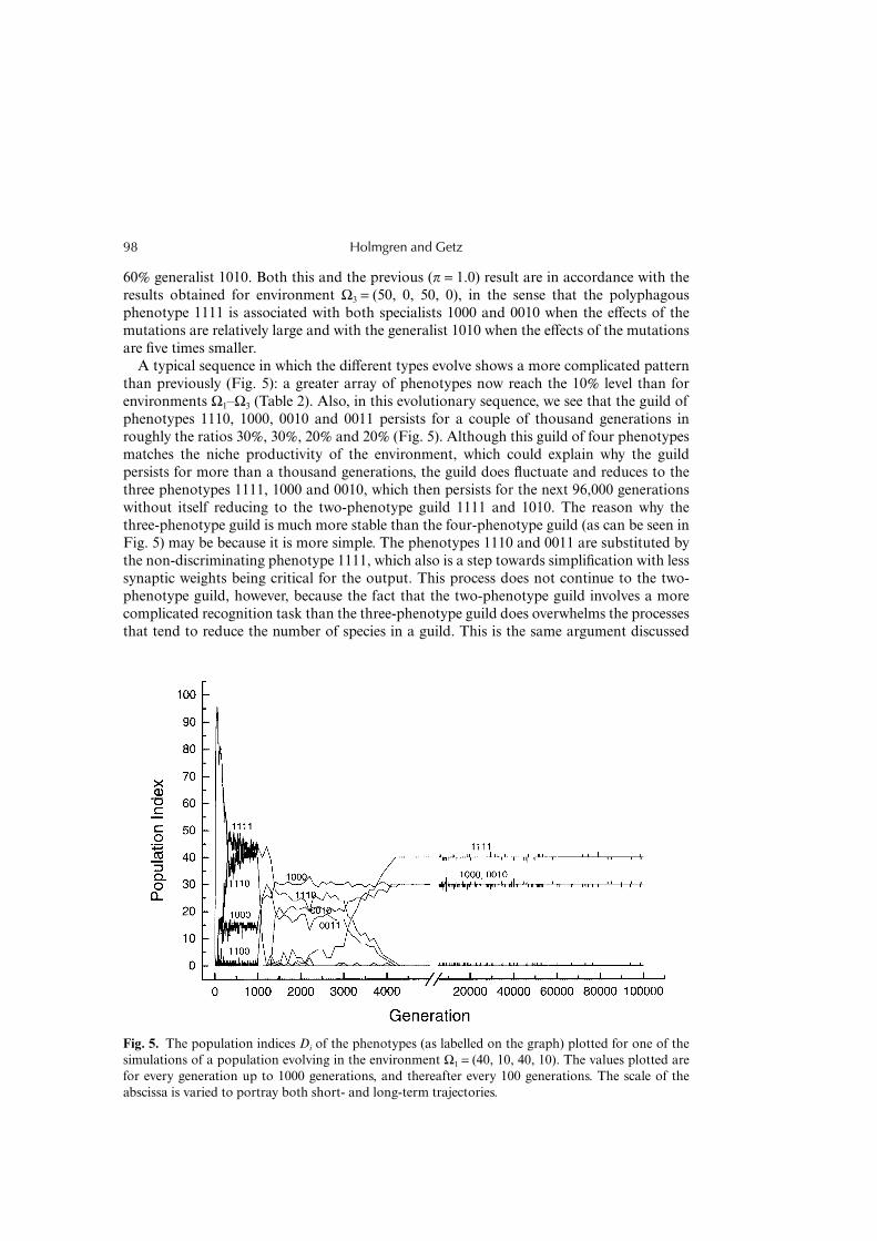
A typical sequence in which the different types evolve shows a more complicated patternthan previously (Fig. 5): a greater array of phenotypes now reach the 10% level than forenvironments Ω1–Ω3 (Table 2). Also, in this evolutionary sequence, we see that the guild ofphenotypes 1110, 1000, 0010 and 0011 persists for a couple of thousand generations inroughly the ratios 30%, 30%, 20% and 20% (Fig. 5). Although this guild of four phenotypesmatches the niche productivity of the environment, which could explain why the guildpersists for more than a thousand generations, the guild does fluctuate and reduces to thethree phenotypes 1111, 1000 and 0010, which then persists for the next 96,000 generationswithout itself reducing to the two-phenotype guild 1111 and 1010. The reason why thethree-phenotype guild is much more stable than the four-phenotype guild (as can be seen inFig. 5) may be because it is more simple. The phenotypes 1110 and 0011 are substituted bythe non-discriminating phenotype 1111, which also is a step towards simplification with lesssynaptic weights being critical for the output. This process does not continue to the two-phenotype guild, however, because the fact that the two-phenotype guild involves a morecomplicated recognition task than the three-phenotype guild does overwhelms the processesthat tend to reduce the number of species in a guild. This is the same argument discussed

Fig. 5. The population indices Di of the phenotypes (as labelled on the graph) plotted for one of thesimulations of a population evolving in the environment Ω1 = (40, 10, 40, 10). The values plotted arefor every generation up to 1000 generations, and thereafter every 100 generations. The scale of theabscissa is varied to portray both short- and long-term trajectories.


in the previous section regarding the stability of the phenotype 1010 compared with the twospecialist phenotypes 1000 and 0010.

Environment 5

When the resource values of the niches are set to be even closer to one another, as inenvironment Ω5 = (30, 20, 30, 20), the stability of different guilds of phenotypes that matchthe environment is reduced and the outcomes less determined after 100,000 generations. Forthe case where the effects of single mutations are relatively small (d = 0.2), 97% of thesimulations do not reach a Nash equilibrium solution after 100,000 generations. For thecase where the effects of single mutations are relatively large (d = 1.0), only 26% of the runsdo not reach a Nash equilibrium. When an equilibrium is reached, the guilds of phenotypesoften do not include specialists: the guild 1111, 1110 and 1011 in the proportions 4 :3 :3 isthe most common (Table 1). In one simulation, however, we see that this guild only arosearound generation 97,000, having previously spent tens of thousands of generations inphenotype guild 1111, 1110, 0011 and 1000 in the proportions 4 :3 :2 :1 (Fig. 6).

Asymmetric niches

Environment 6

We also investigated evolution in the asymmetric environment Ω6 = (60, 0, 40, 0). In thiscase, it is no longer possible for the generalist phenotype 1010 to efficiently exploit the

Fig. 6. The population indices Di of the phenotypes (as labelled on the graph) plotted for one of thesimulations of a population evolving in the environment Ω1 = (30, 20, 30, 20). The values plotted arefor every generation up to 1000 generations, and thereafter every 100 generations. The scale of theabscissa is varied to portray both short- and long-term trajectories.

Holmgren and Getz100

environment on its own. Thus we see the appearance of the Nash equilibrium solutioninvolving the generalist 1010 and specialist 1000 in an 8 :2 mix. In all cases, however, a 6 :4mix of the two specialists provided the most common matching of the plant resourcedistribution (Table 1).

The number of simulations that do not reach a Nash equilibrium is almost identical tothe case Ω3 = (50, 0, 50, 0) (1 vs 2 when (π, d ) = (0.1, 1.0); 9 vs 11 when (π, d ) = (0.02, 1.0);24 vs 21 when (π, d ) = (0.1, 0.2); and 45 vs 42 when (π, d ) = (0.2, 0.02)). Thus the asymmetryin question does not affect the rate at which phenotype guilds evolved to Nash equilibria,only that generalists are much less likely to evolve in the asymmetric than in the symmetriccase when the rate of evolution is comparatively low (for the case (π, d ) = (0.2, 0.02),54% generalists evolved in the symmetric case while no guilds containing generalistsevolved in the asymmetric case). When the generalist evolves, the specialist 1000 will need tobe retained at the level of 20% of the population to provide the necessary competitivebalance in the more productive plant niche (which is the first or Type 1). It is now likely thatthe other specialist 0010 evolves from the generalist, and the two specialists will take overdue to the stability argument made earlier. In environment Ω3, both specialists have toevolve from the generalist more or less simultaneously, something which is less likely com-pared to when the specialists can evolve sequentially as is the case here in environment Ω6.

DISCUSSION

Although our model is a parody of perceptual, ecological and selective processes thatmould the form of individual organisms, like all models in population biology it provides uswith a tool for generating ideas and investigating the complexities of the evolutionaryprocess in question. In particular, our model enables us, for the first time, to explore in depththe evolution under perceptual constraints of host-plant range in phytophagous insects.

Several selective and non-selective factors have been proposed that affect host-plantrange in phytophagous insects (for a review, see Bernays and Chapman, 1994). Thesefactors include resource availability, interspecific competition, climate, chemical defencesin plants, neurological constraints, other morphological constraints, and phenologicalconstraints. Regardless of the ultimate factors of the evolution of host-plant range, ‘theevolution of behavioral patterns is the evolution of properties of the neural system’(Bernays and Chapman, 1994).

The apparent suboptimal behaviour that many insects exhibit in ignoring ubiquitousresources that would contribute greatly to their fitness is explainable in terms of the hypo-thesis that the evolution of feeding behaviour in insects is constrained by perceptual andmemory considerations. Arguments in support of this hypothesis have been made (Fox,1993; Bernays and Wcislo, 1994), including a thorough discussion by Fox and Lalonde(1993) of the information-processing limitations inherent in olfactory perception (see alsoGetz and Page, 1991).

Most neurological constraint models that have been proposed in the literature assumethat the herbivore does not have the neural capacity to be a competent generalist. Levinsand MacArthur (1969), for example, assumed that herbivores are unable to include a newbeneficial host in their diet without increasing the probability of including hosts that wouldincur some cost to fitness. Schneider (1987) suggested that a herbivore’s image of its hostplants becomes more ‘blurred’ as the range of hosts increases. A similar idea was presentedby Bernays and Wcislo (1994), who suggested that herbivores that were ‘focusing’ on fewer


host-plants had better recognition performance. Fox and Lalonde (1993) also made thisassumption of the imperfect generalist. Although these ideas have some validity, our studywas not constrained by a network being insufficiently complex to perform the perceptualtask required to be a generalist.

Our results take us a step further in evaluating the effects that perceptual constraintsmight have on the evolutionary dynamics of plant-feeding insect guilds. The results indicatethat implementation of host-plant recognition in neurological structures may bias theevolution towards specialists or generalists. Hence, our work focuses on the likelihoodthat evolution will take a particular path rather than on the selective forces themselves. Inour system, the driving force of evolution is competition for a share of the resourcesprovided by each plant. This force does not a priori favour generalists or specialists. Thefitness of a given phenotype is dependent on the mix of extant phenotypes competingfor the different resources. The emergence of a phenotype depends on the difficulty ofthe discrimination task required to express that phenotype (a more difficult task being morelevels of discrimination that must be implemented by the network). The maintenanceof a phenotype depends on the stability of the guild of phenotypes and how easily thatguild is disrupted by the invasion of other phenotypes. Our results suggest generalizationsthat may well apply to an array of systems that deal with the question of evolution of nicheselection.

Obviously, the simulations we present cannot be construed to mimic the actual phylogenyof feeding behaviour in any real insect clade: our model is far too simple for that. Rather,our results reveal mechanisms or rules that help us resolve the apparent suboptimality ofcurrently observed feeding preferences in a number of species, as well as suggest hypothesesfor explaining the phylogeny of diet breadth in particular clades. From our results, wepropose that the following three rules have a strong influence on feeding preference, and arecritical in determining whether generalists or specialists will evolve. These rules may alsohelp explain the mix of phenotypes observed in stable guilds of herbivorous insectsexploiting a heterogeneous environment of plant types:

1. The probability associated with the emergence of a particular phenotype depends bothon the mix of extant phenotypes and on the difficulty of the perceptual task.

2. Guilds (of one or several phenotypes) may be displaced by more fit guilds until theresource utilization by the guild matches the relative availability of resources of varyingquality (Nash equilibrium: Bulmer, 1994).

3. Guilds at the Nash equilibrium may be displaced by other more stable Nash equilibria,especially if mutation rates are high.

The essence of Rule 1 in the context of neural networks is that phenotypes solvingrelatively simple recognition or discrimination tasks evolve before phenotypes solving morecomplex recognition or discrimination tasks. This is certainly borne out by the results inTables 2–4. The reason for this could be that the number of ways a feedforward network isable to solve a recognition task decreases with the difficulty of the task. Thus, the morepossible configurations of synapse weights that lead to the emergence of a particular pheno-type, the earlier we can expect that phenotype to evolve. There are exceptions to this generaltrend, for example the generalist 1010 in environments Ω3–Ω6, where the generalist appearsrelatively early. We interpret this as an increased probability for this type to evolve fromintermediate types (i.e. the generalist phenotype 1010 is more likely to evolve from the


prevailing specialist 1000 than the specialist phenotype 0010 is) and, therefore, the result stillobeys the extant phenotype component of Rule 1. We regard the order of appearance ofphenotypes as the main explanatory factor in our results. The order of appearance deter-mines the outcome of two competing guilds (e.g. specialists versus a generalist) having thesame fitness from an optimization point of view – the first guild to evolve will often resistinvasion by the other guilds (see asterisks in Tables 2–4). If a new guild is to be established,first all new guild members need to evolve from the existing phenotypes more or less simul-taneously to displace the existing guild. This becomes more unlikely with an increasingnumber of new guild members. Second, the new guild has to be more successful than theextant one in order to spread. This is determined by Rules 2 and 3.

The importance of Rule 2 is evident from the results in Table 1, where we see that thefrequencies of phenotypes in different guilds equilibrate at proportions that correspond toan ideal free distribution. Rule 2, however, not only has something to say about the finaloutcome of evolution, but also about the process, since the fitness of a phenotype at anypoint in time is affected by the distribution of other phenotypes at that point in time. Thisfact is dramatically illustrated in Fig. 3, where, although the proportion of specialists togeneralists drifts through time on a low-resolution time scale (right-hand side of Fig. 3),the proportions of the two specialists are indistinguishable over time from one another.Furthermore, the rate of drift is remarkably slow (note the unit of time illustrated on theright-hand side of Fig. 3 is 10,000 generations). The reason for this slowness is thatthe proportions of the two specialists have to drift in concert subject to the constraint thatthe whole guild of phenotypes constitutes an ideal free distribution.

Rule 3, as with Rule 1, pertains to the degree of difficulty of recognition task performedby phenotypes and even guilds. The greater the number of levels of categorization, the morelikely that each individual synapse weight is critical, and hence the more likely that muta-tions are deleterious. This fact is most clearly visualized in Fig. 5. Here we see a Nashequilibrium guild consisting of four phenotypes emerging after about 1300 generations. Therelative frequencies of the phenotypes are quite unstable, and do not stabilize until two ofthe phenotypes have been substituted by a single new phenotype. Naturally, Rule 3 becomesmore important with increasing effects of mutations, which is exemplified by the shift fromgeneralist to specialists in environments Ω3 and Ω4 (Table 1).

We may make some conclusions regarding the comparison of our results in the differentenvironments. Environments Ω1–Ω3 represent increasing difficulty for a generalist to recog-nize its plants, whereas this is not true for the specialists. For reasons explained above, wesee that the more complex the environment, the more likely that specialization will be thedominant strategy. If environment Ω3 is changed so that the completely non-valuable plantsare of some low value as a resource to the herbivores, we get environments Ω4 and Ω5.In these environments, the evolving guilds consist of a larger number of specialistscompared to environment Ω3. When plants become more similar in resource value, as inenvironment Ω5 compared to environment Ω4, it seems that the guilds are more likely toconsist of generalists (compare most common equilibria for these environments in Table 1).Asymmetry also seems to favour the evolution of specialization (environment Ω6). Sincemost environments are likely to exhibit at least a moderate degree of asymmetry in theavailability of plants of differing quality, we should rarely see generalists on their own,but most often in association with one or more specialists exploiting the plant nichesthat are most under-utilized by the generalist. To express this in another way, it may bedifficult for generalists to evolve to match the ideal free distribution of a heterogeneous


environment, thereby providing opportunities for the evolution of specialists on the leastefficiently utilized plants.

Our model suggests that three types of clades of herbivores are most likely to evolve: (a)monophages or specialists, (b) oligophages that feed on a related group of plants with asimilar odour signature, and (c) non-discriminating heterophages. In other words, ourmodel suggests that oligophages or heterophages will not omit nutritive plants from theirdiet that have signatures intermediate between plants upon which they feed. These pre-dictions fit with the observation that natural clades of insect species are, primarily, mono- oroligophagous on distantly related plants. The most common situation is oligophagousclades living on a restricted group of plant species (Jermy, 1984).

In our model, we have assumed that the values of the network parameters are subject tomutation and are heritable, but are not plastic within each generation. We expect, however,that Rules 1–3 could also apply when learning takes place within networks over the lifetimeof an individual, because parameter adjustments in neural networks can be used to modellearning over both intra- and inter-generational time scales. We therefore expect that factorselucidated by our analysis have some validity for niche selection on ecological as wellevolutionary time scales.

In conclusion, our results provide us with insights into how particular guilds of specialistand generalist plant feeding phenotypes may be influenced by perceptual constraints. First,our model clearly demonstrates that perceptual constraints influence the order in whichparticular phenotypes appear – the easier the perceptual task, the earlier that phenotypeappears – and that this order is critical in determining the guild of phenotypes that assembleand persist for some period of time. Thus, in any real system, some understanding of why aparticular guild exists will arise from insights into the difficulties of the perceptual tasksassociated with particular phenotypes. With hindsight, this insight seems obvious. Lessobvious is the insight that guilds with several phenotypes arise and persist for long periodsof time, but are eventually replaced in a saltatorial manner by guilds that are more stable.This suggests that many extant guilds of herbivorous insects are not necessarily the mostoptimal long-term configurations. Whether the most stable configurations ultimately evolvedepends on whether the background environment remains constant for long enough toprevent extant configurations from being disrupted. Finally, the model suggests two reasonswhy specialization is the dominant strategy in insect communities: the required neuralsettings for specialists are easier to evolve and are more resistant to mutations (in a generalsense) compared with generalists. Specialists are required in guilds to make up an ‘ideal free’matching to the resource values of the host plants.

ACKNOWLEDGEMENTS

This study received support from Per Erik Lindahl’s Foundation (The Swedish Royal Academy ofSciences) and Wennergren Center to N.H. and funding from the University of California AgriculturalExperiment Station to W.M.G. We thank Elizabeth Bernays, Magnus Enquist, William Lemon,Rainer Malaka and four anonymous referees for comments and suggestions that improved themanuscript.

REFERENCES

Berenbaum, M.R. 1996. Introduction to the symposium: On the evolution of specialization. Am.Nat., 148 (suppl.): S78–S83.


Bernays, E.A. 1998. The value of being a resource specialist: Behavioral support for a neuralhypothesis. Am. Nat., 151: 451–464.

Bernays, E.A. and Chapman, R.F. 1978. Plant chemistry and acridoid feeding behavior. In Bio-chemical Aspects of Plant and Animal Coevolution (J.B. Harbone, ed.), pp. 99–141. London:Academic Press.

Bernays, E.A. and Chapman, R.F. 1994. Host-Plant Selection by Phytophagous Insects. Con-temporary Topics in Entomology 2. New York: Chapman & Hall.

Bernays, E.A. and Graham, M. 1988. On the evolution of host specificity in phytophagousarthropods. Ecology, 69: 886–892.

Bernays, E.A. and Wcislo, W.T. 1994. Sensory capabilities, information processing, and resourcespecialization. Q. Rev. Biol., 69: 187–204.

Brown, J.S. and Vincent, T.L. 1987. A theory for the evolutionary game. Theor. Pop. Biol., 31:140–166.

Bulmer, M.G. 1994. Theoretical Evolutionary Ecology. Sunderland, MA: Sinauer Associates.Chapman, R.F. 1988. Sensory aspects of host-plant recognition by Acrodiodea: Questions

associated with the multiplicity of receptors and variability of response. J. Insect Physiol., 34:167–174.

Christiansen, F.B. 1975. Hard and soft selection in a subdivided population. Am. Nat., 109:11–16.

DeAngelis, D.L. and Gross, L.J. 1992. Individual-based Models and Approaches in Ecology.New York: Chapman & Hall.

Dempster, E.R. 1955. Maintenance of genetic heterogeneity. Cold Spring Harbor Symp. Quant. Biol.,20: 25–32.

Dickinson, J.L., Koenig, W.D. and Pitelka, F.A. 1996. Fitness consequences of helping behavior inthe western bluebird. Behav. Ecol., 7: 168–177.

Dukas, R.R. and Real, L.A. 1991. Learning foraging tasks by bees: A comparison between socialand solitary species. Anim. Behav., 42: 269–276.

Dukas, R.R. and Real, L.A. 1993. Cognition in bees: From stimulus reception to behavioral change.In Insect Learning (D.R.L. Papaj, ed.), pp. 343–373. New York: Chapman & Hall.

Enquist, M. and Arak, A. 1994. Symmetry, beauty and evolution. Nature, 372: 169–172.Feeny, P.P. 1987. The roles of plant chemistry in associations between swallowtail butterflies and

their host plants. In Insects–Plants: Proceedings of the 6th International Symposium on Insect–Plant Relationships (PAU 1986) (V. Labeyrie, G. Fabres and D. Lachaise, eds), pp. 353–359.Dordrecht: W. Junk Publishers.

Fox, C.W.L. and Lalonde, R.G. 1993. Host confusion and the evolution of insect diet breadths.Oikos, 67: 577–581.

Fretwell, S.D. and Lucas, H.L. 1970. On territorial behaviour and other factors influencing habitatdistribution in birds. Acta Biotheor., 19: 16–36.

Futuyma, D.J. 1991. Evolution of host specificity in herbivorous insects: Genetic, ecological,and phylogenetic aspects. In Plant–Animal Interactions: Evolutionary Ecology in Tropical andTemperate Regions (P.W. Price, T.M. Lewinsohn, G.W. Fernandes and W.W. Benson, eds),pp. 431–454. New York: John Wiley.

Futuyma, D.J. and Moreno, G. 1988. The evolution of ecological specialization. Ann. Rev. Ecol.Syst., 19: 207–233.

Futuyma, D.J., Keese, M.C. and Scheffer, S.J. 1993. Genetic constraints and the phylogeny ofinsect–plant associations – responses of Ophraella communa (Coleoptera, Chrysomelidae) to hostplants of its congeners. Evolution, 47: 888–905.

Futuyma, D.J., Keese, M.C. and Funk, D.J. 1995. Genetic constraints on macroevolution – theevolution of affiliation in the leaf beetle genus Ophraella. Evolution, 49: 797–809.

Getz, W.M. 1996. A hypothesis regarding density dependence and the growth rate of populations.Ecology, 77: 2014–2026.


Getz, W.M. 1999. Population and evolutionary dynamics of consumer-resource systems. InAdvanced Ecological Theory: Principles and Applications (J. McGlade, ed.), pp. 194–231. Oxford:Blackwell Scientific.

Getz, W.M. and Akers, R.P. 1993. Olfactory response characteristics and tuning structure ofplacodes in the honey bee Apis mellifera L. Apidologie, 24: 195–217.

Getz, W.M. and Kaitala, V. 1989. Ecogenetic models, competition, and heteropatry. Theor. Pop.Biol., 36: 34–58.

Getz, W.M. and Page, R.E., Jr. 1991. Chemosensory kin-communication systems and kinrecognition in Honey bees. Ethology, 87: 298–315.

Hammer, M. and Menzel, R. 1995. Learning and memory in the honeybee. J. Neurosci., 15:1617–1630.

Haykin, S. 1994. Neural Networks: A Comprehensive Foundation. New York: Macmillan CollegePublishing.

Janz, N. and Nylin, S. 1997. The role of female search behaviour in determining host plant rangein plant feeding insects: A test of the information processing hypothesis. Proc. R. Soc. Lond. B,264: 701–707.

Jermy, T. 1984. Evolution of insect/host plant relationships. Am. Nat., 124: 609–630.Kaitala, V. and Getz, W.M. 1995. Population dynamics and harvesting of semelparous species with

phenotypic and genotypic variability in reproductive age. J. Math. Biol., 33: 521–556.Laurent, G. 1996. Dynamical representation of odors by oscillating and evolving neural assemblies.

TINS, 19: 489–496.Lemon, W.C. and Getz, W.M. 1999. Olfactory coding in insects. Ann. Ent. Soc. Am., 92: 861–872.Levene, H. 1953. Genetic equilibrium when more than one ecological niche is available. Am. Nat., 87:

331–333.Levins, R. and MacArthur, R. 1969. An hypothesis to explain the incidence of monophagy. Ecology,

50: 910–911.Lindgren, K. 1990. Evolution in a population of mutating strategies. NORDITA Preprint, 90/225.Masson, C. and Mustaparta, H. 1990. Chemical information processing in the olfactory system of

insects. Physiol. Rev., 70: 199–245.Maynard Smith, J. 1982. Evolution and the Theory of Games. Cambridge: Cambridge University Press.Nash, J.F. 1951. Non-cooperative games. Ann. Math., 54: 286–295.Olías, J.M., Pérez, A.G., Ríos, J.J. and Sanz, L.C. 1993. Aroma of olive virgin oil: Biogenesis of the

‘green’ odor notes. Agric. Food Chem., 41: 2368–2373.Parker, G.A. 1970. The reproductive behaviour and the nature of sexual selection in Scatophaga

stercoraria L. (Diptera: Scatophagidae). II. The fertilization rate and the spatial and temporalrelationships of each sex around the site of mating and oviposition. J. Anim. Ecol., 39: 205–228.

Parker, G.A. and Sutherland, W.J. 1986. Ideal free distributions when individuals differ in competi-tive ability: Phenotype limited ideal free models. Anim. Behav., 34: 1222–1242.

Schneider, D. 1987. Plant recognition by insects: A challenge to neuroethological research. InInsects–Plants: Proceedings of the 6th International Symposium on Insect–Plant Relationships(PAU 1986) (V. Labeyrie, G. Fabres and D. Lachaise, eds), pp. 117–123. Dordrecht: W. JunkPublishers.

Smith, B.H. and Getz, W.M. 1994. Nonpheromonal olfactory processing in insects. Ann. Rev.Entomol., 39: 351–375.

Swain, T. 1977. Secondary plant compounds as protective agents. Ann. Rev. Plant Physiol., 42:255–302.

Taylor, P.D. 1989. Evolutionary stability in one-parameter models under weak selection. Theor. Pop.Biol., 36: 125–143.

Vincent, T.L. and Brown, J.S. 1988. The evolution of ESS theory. Ann. Rev. Ecol. Syst., 19:423–443.

Visser, J.H. 1986. Host odor perception in phytophagous insects. Ann. Rev. Entomol., 31: 121–144.


Visser, J.H. and de Jong, R. 1987. Plant odour perception in the Colorado potato beetle:Chemoattraction towards host plants. In Insects–Plants: Proceedings of the 6th InternationalSymposium on Insect–Plant Relationships (PAU 1986) (V. Labeyrie, G. Fabres and D. Lachaise,eds), pp. 129–134. Dordrecht: W. Junk Publishers.

Evolution of host plant selection in insects under...

Documents

Transcript of Evolution of host plant selection in insects under...