Evolution Models for Mass

Transportation Problems

Giuseppe Buttazzo

Dipartimento di Matematica

Universita di Pisa

buttazzo@dm.unipi.it

http://cvgmt.sns.it

“MEAN FIELD GAMES AND RELATED TOPICS”Rome, May 12-13, 2011

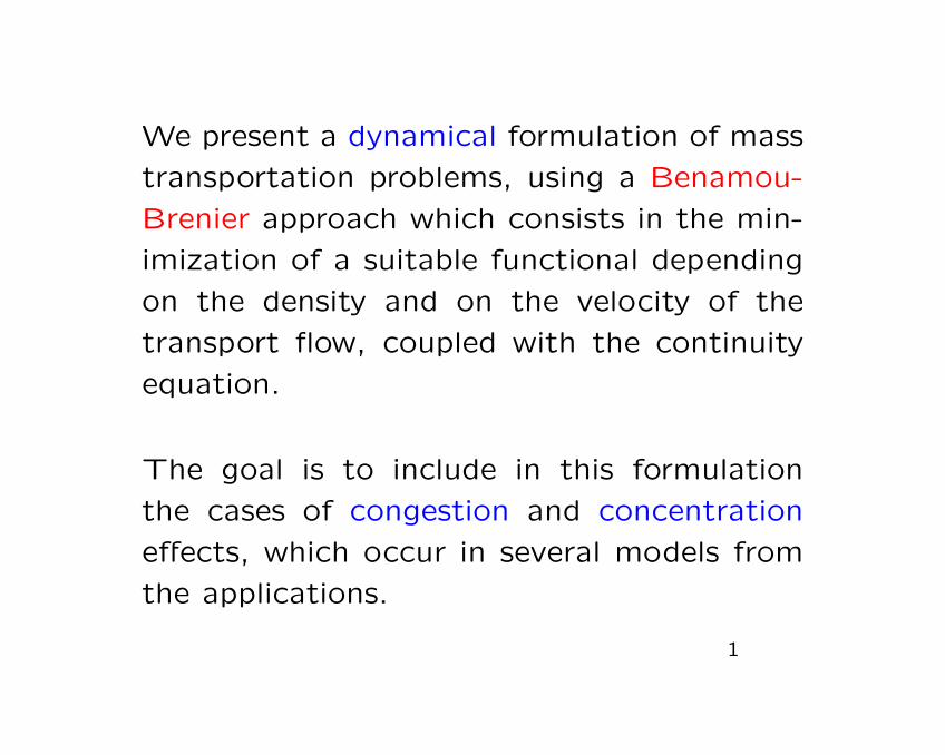
We present a dynamical formulation of mass

transportation problems, using a Benamou-

Brenier approach which consists in the min-

imization of a suitable functional depending

on the density and on the velocity of the

transport flow, coupled with the continuity

equation.

The goal is to include in this formulation

the cases of congestion and concentration

effects, which occur in several models from

the applications.

1

• Congestion effects for instance occur in

the simulation of traffic flows with high den-

sity and of movement of crowds under panic

effects.

Due to the congestion, the transport rays

tend to be far each other.

• Concentration effects for instance occur in

several models of branching transportation,

as roots of trees, roads, communication net-

works, delta of rivers, blood vessels.

2

The main tool is a good comprehension of

lower semicontinuous functionals defined on

the space of measures, studied in a series of

papers by Bouchitte-Buttazzo:

• Nonlinear Anal. 1990

• Ann.IHP Anal.NonLin. 1992

• Ann.IHP Anal.NonLin. 1993

Applications to mass transportation problems:

Brancolini-Buttazzo-Santambrogio JEMS 2006

Buttazzo-Jimenez-Oudet SIAM JCO 2009

Brasco-Buttazzo-Santambrogio preprint 2010

available at http://cvgmt.sns.it

3

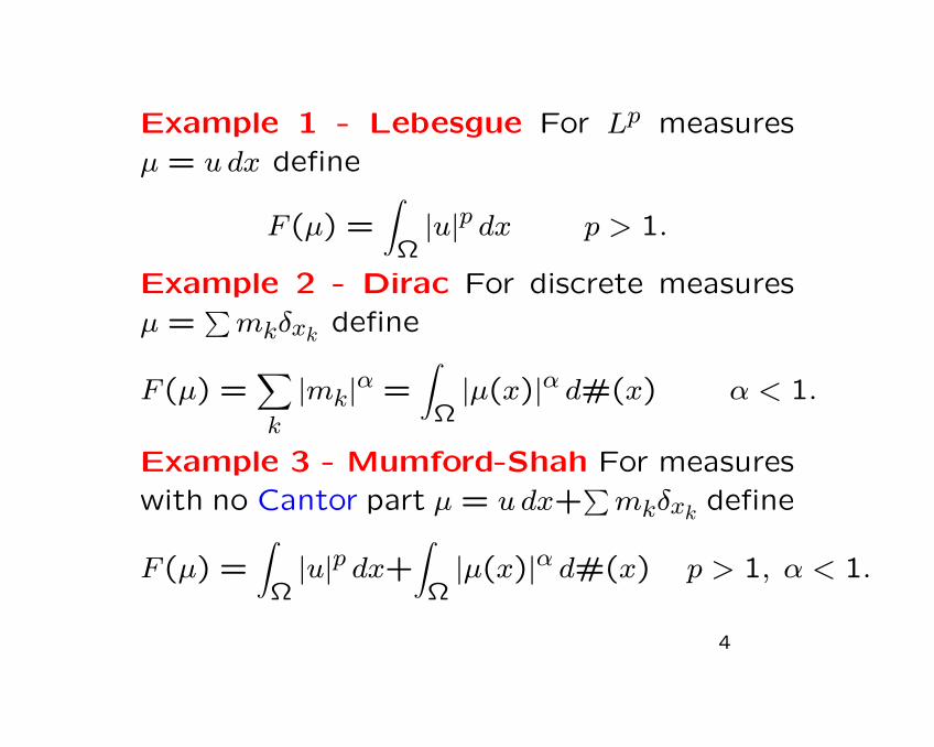
Example 1 - Lebesgue For Lp measuresµ = u dx define

F (µ) =∫

Ω|u|p dx p > 1.

Example 2 - Dirac For discrete measuresµ =

∑mkδxk define

F (µ) =∑k

|mk|α =∫

Ω|µ(x)|α d#(x) α < 1.

Example 3 - Mumford-Shah For measureswith no Cantor part µ = u dx+

∑mkδxk define

F (µ) =∫

Ω|u|p dx+

∫Ω|µ(x)|α d#(x) p > 1, α < 1.

4

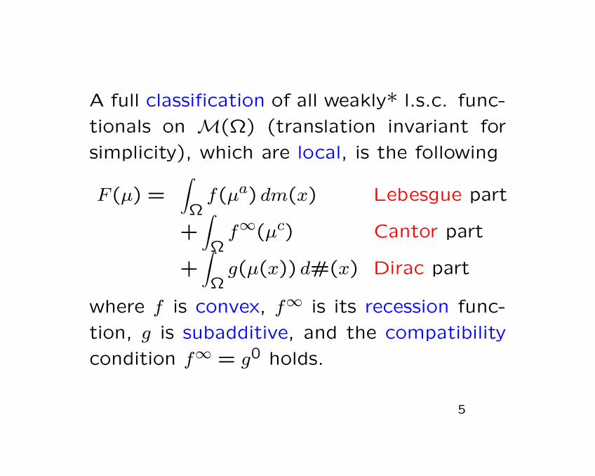
A full classification of all weakly* l.s.c. func-

tionals on M(Ω) (translation invariant for

simplicity), which are local, is the following

F (µ) =∫

Ωf(µa) dm(x) Lebesgue part

+∫

Ωf∞(µc) Cantor part

+∫

Ωg(µ(x)) d#(x) Dirac part

where f is convex, f∞ is its recession func-

tion, g is subadditive, and the compatibility

condition f∞ = g0 holds.

5

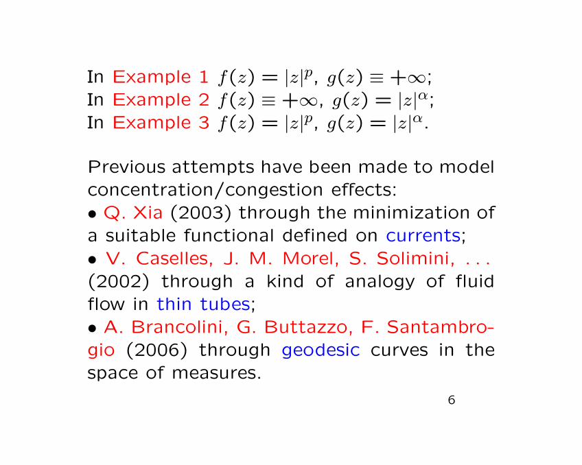
In Example 1 f(z) = |z|p, g(z) ≡ +∞;In Example 2 f(z) ≡ +∞, g(z) = |z|α;In Example 3 f(z) = |z|p, g(z) = |z|α.

Previous attempts have been made to modelconcentration/congestion effects:• Q. Xia (2003) through the minimization ofa suitable functional defined on currents;• V. Caselles, J. M. Morel, S. Solimini, . . .(2002) through a kind of analogy of fluidflow in thin tubes;• A. Brancolini, G. Buttazzo, F. Santambro-gio (2006) through geodesic curves in thespace of measures.

6

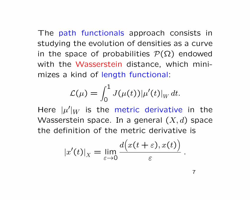
The path functionals approach consists instudying the evolution of densities as a curvein the space of probabilities P(Ω) endowedwith the Wasserstein distance, which mini-mizes a kind of length functional:

L(µ) =∫ 1

0J(µ(t))|µ′(t)|W dt.

Here |µ′|W is the metric derivative in theWasserstein space. In a general (X, d) spacethe definition of the metric derivative is

|x′(t)|X = limε→0

d(x(t+ ε), x(t)

)ε

.

7

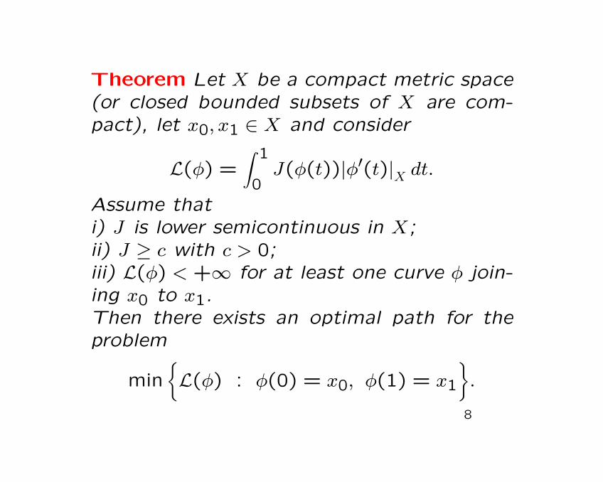
Theorem Let X be a compact metric space(or closed bounded subsets of X are com-pact), let x0, x1 ∈ X and consider

L(φ) =∫ 1

0J(φ(t))|φ′(t)|X dt.

Assume thati) J is lower semicontinuous in X;ii) J ≥ c with c > 0;iii) L(φ) < +∞ for at least one curve φ join-ing x0 to x1.Then there exists an optimal path for theproblem

minL(φ) : φ(0) = x0, φ(1) = x1

.

8

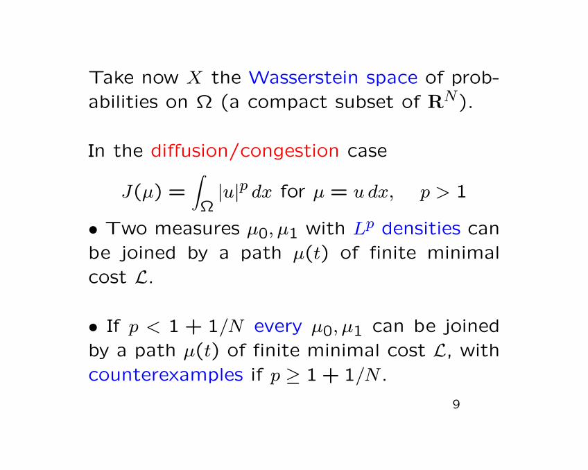
Take now X the Wasserstein space of prob-abilities on Ω (a compact subset of RN).

In the diffusion/congestion case

J(µ) =∫

Ω|u|p dx for µ = u dx, p > 1

• Two measures µ0, µ1 with Lp densities canbe joined by a path µ(t) of finite minimalcost L.

• If p < 1 + 1/N every µ0, µ1 can be joinedby a path µ(t) of finite minimal cost L, withcounterexamples if p ≥ 1 + 1/N .

9

In the concentration/branching case:

J(µ) =∑k

|mk|α for µ =∑

mkδxk, α < 1

• Two discrete measures µ0, µ1 can be joined

by a path µ(t) of finite minimal cost L.

• If α > 1 − 1/N every µ0, µ1 can be joined

by a path µ(t) of finite minimal cost L, with

counterexamples if α ≤ 1− 1/N .

10

A coefficient J(µ) of Lebesgue type thenprovides a congestion functional, while J(µ)of Dirac type gives a model for describingconcentrations.

Some refinements of the path theory ap-proach have been made in:

L. Brasco, F. Santambrogio DCDS (2011)

L. Brasco Ann. Mat. Pura Appl. (2010)

L. Brasco Ph.D. Thesis, U.Pisa + U.Paris-Dauphine, 2010.

11

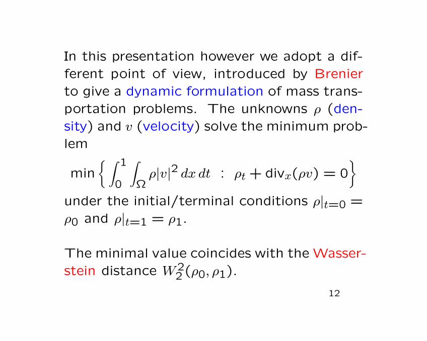
In this presentation however we adopt a dif-ferent point of view, introduced by Brenierto give a dynamic formulation of mass trans-portation problems. The unknowns ρ (den-sity) and v (velocity) solve the minimum prob-lem

min ∫ 1

0

∫Ωρ|v|2 dx dt : ρt + divx(ρv) = 0

under the initial/terminal conditions ρ|t=0 =ρ0 and ρ|t=1 = ρ1.

The minimal value coincides with the Wasser-stein distance W2

2 (ρ0, ρ1).

12

Setting ρv = q the continuity equation be-comes linear:

ρt + divx q = 0

and the cost functional (representing the ki-netic energy) becomes convex:∫ 1

0

∫Ω

|q|2

ρdx dt.

To be precise, the correct meaning has to begiven in terms of measures:∫ 1

0

∫Ω

∣∣∣∣dqdρ∣∣∣∣2 dρ(x) dt.

13

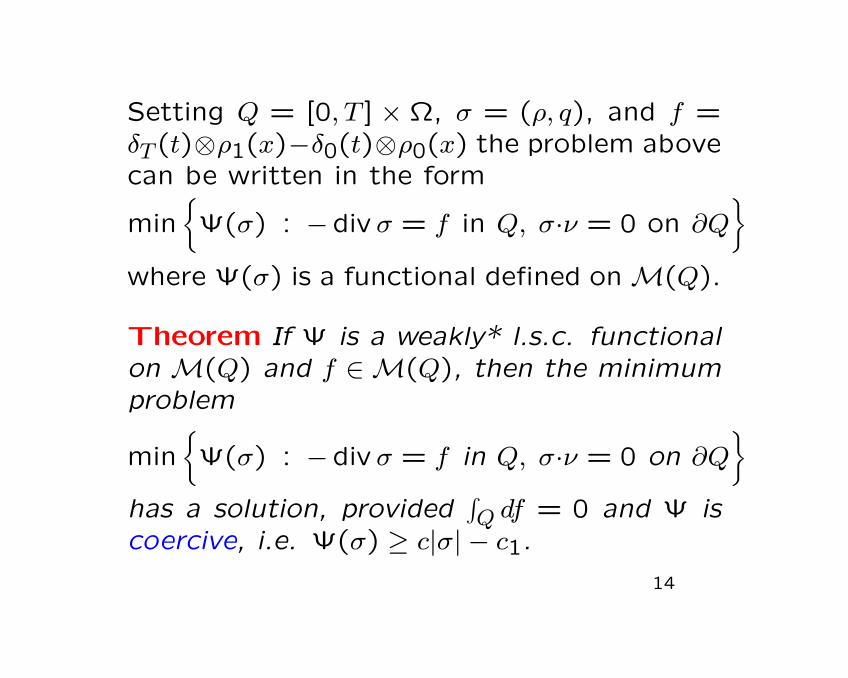
Setting Q = [0, T ] × Ω, σ = (ρ, q), and f =δT (t)⊗ρ1(x)−δ0(t)⊗ρ0(x) the problem abovecan be written in the form

min

Ψ(σ) : −div σ = f in Q, σ·ν = 0 on ∂Q

where Ψ(σ) is a functional defined onM(Q).

Theorem If Ψ is a weakly* l.s.c. functionalon M(Q) and f ∈M(Q), then the minimumproblem

min

Ψ(σ) : −div σ = f in Q, σ·ν = 0 on ∂Q

has a solution, provided

∫Q df = 0 and Ψ is

coercive, i.e. Ψ(σ) ≥ c|σ| − c1.14

The functionals Ψ we have in mind are of

the form

Ψ(σ) =∫ T

0J(σ(t)

)dt

and again J of Lebesgue type would provide

congestion models, while J of Dirac type

would provide concentration models.

The congestion case is simpler, because the

functional J is convex. The concentration

case, on the contrary, requires some extra

analysis, due to concavity effects.

15

Dual formulation (in the convex case):

sup〈f, φ〉 −Ψ∗(Dφ) : φ ∈ C1(Q)

.

Primal-dual relation:

Ψ(σopt) + Ψ∗(Dφopt) = 〈σopt, Dφopt〉.

The point is that the maximizer in the dual

formulation is not of class C1 in general. A

relaxation formula is then needed for Ψ∗ to

extend it to its natural space.

16

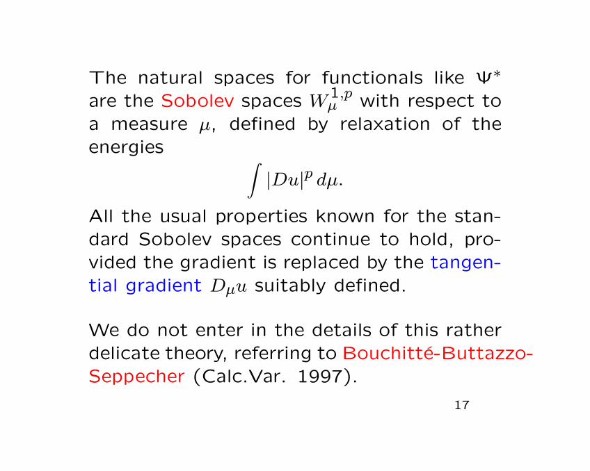
The natural spaces for functionals like Ψ∗

are the Sobolev spaces W1,pµ with respect to

a measure µ, defined by relaxation of theenergies ∫

|Du|p dµ.

All the usual properties known for the stan-dard Sobolev spaces continue to hold, pro-vided the gradient is replaced by the tangen-tial gradient Dµu suitably defined.

We do not enter in the details of this ratherdelicate theory, referring to Bouchitte-Buttazzo-Seppecher (Calc.Var. 1997).

17

The numerical approximation has been per-formed in [BJO] following the scheme usedin Benamou-Brenier, through an augmentedLagrangian algorithm. The following anima-tions deal with a domain Ω not convex (akind of subway gate) and with the cases:

• J(ρ, q) = |q|2ρ in which the transportation

simply follows the Wasserstein geodesics.• J(ρ, q) = |q|2

ρ +cρ2 in which the Wassersteintransportation is perturbed by the additionof a diffusion term (panic effect).

• J(ρ, q) = |q|2ρ + χρ≤M in which there is

the additional constraint that two differentindividual do not want to stay too close.

18

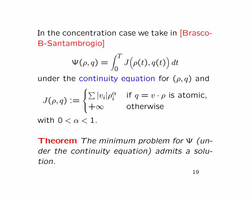
In the concentration case we take in [Brasco-B-Santambrogio]

Ψ(ρ, q) =∫ T

0J(ρ(t), q(t)

)dt

under the continuity equation for (ρ, q) and

J(ρ, q) :=

∑|vi|ραi if q = v · ρ is atomic,

+∞ otherwise

with 0 < α < 1.

Theorem The minimum problem for Ψ (un-der the continuity equation) admits a solu-tion.

19

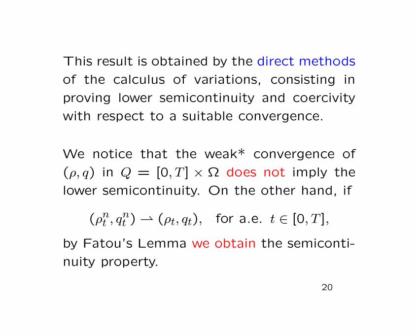
This result is obtained by the direct methods

of the calculus of variations, consisting in

proving lower semicontinuity and coercivity

with respect to a suitable convergence.

We notice that the weak* convergence of

(ρ, q) in Q = [0, T ] × Ω does not imply the

lower semicontinuity. On the other hand, if

(ρnt , qnt ) (ρt, qt), for a.e. t ∈ [0, T ],

by Fatou’s Lemma we obtain the semiconti-

nuity property.

20

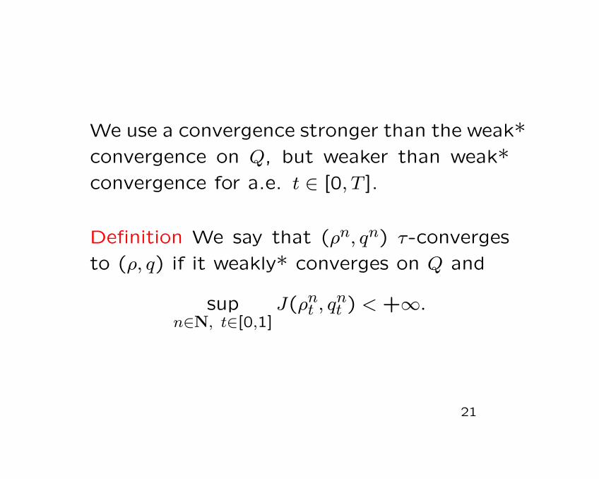
We use a convergence stronger than the weak*

convergence on Q, but weaker than weak*

convergence for a.e. t ∈ [0, T ].

Definition We say that (ρn, qn) τ-converges

to (ρ, q) if it weakly* converges on Q and

supn∈N, t∈[0,1]

J(ρnt , qnt ) < +∞.

21

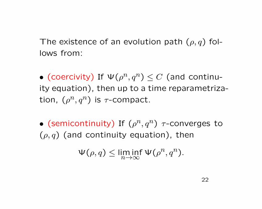
The existence of an evolution path (ρ, q) fol-

lows from:

• (coercivity) If Ψ(ρn, qn) ≤ C (and continu-

ity equation), then up to a time reparametriza-

tion, (ρn, qn) is τ-compact.

• (semicontinuity) If (ρn, qn) τ-converges to

(ρ, q) (and continuity equation), then

Ψ(ρ, q) ≤ lim infn→∞ Ψ(ρn, qn).

22

The evolution model above is “equivalent”

to the static ones by Gilbert, Xia, Bernot-

Caselles-Morel, in the sense that the two

minima coincide and there is a natural way

to pass from a dynamic minimizer of our

problem to a static minimizer of the previous

models.

Some numerical computations have been made

by E. Oudet and can be found on his web

page:

http://www.lama.univ-savoie.fr/~oudet/

23

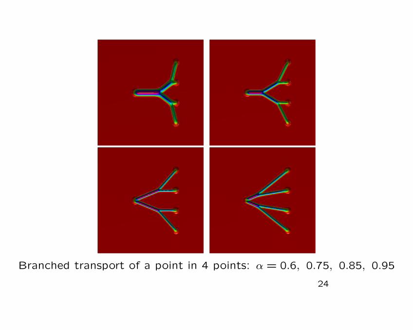
Branched transport of a point in 4 points: α = 0.6, 0.75, 0.85, 0.95

24

Branched transport of a point in a circle: α = 0.6, 0.75, 0.85, 0.95

25