EVIM: A Software Package for Extreme Value Analysis in MATLABrgencay/evim.pdf · EVIM: A Software...

EVIM: A Software Package for Extreme Value Analysis in MATLAB

Ramazan Gencay

Department of EconomicsUniversity of [email protected]

Faruk Selcuk

Department of EconomicsBilkent University

[email protected]

Abdurrahman Ulugulyagcı

Department of EconomicsBilkent University

[email protected]

Abstract. From the practitioners’ point of view, one of the most interesting questions that tail studies can

answer is what are the extreme movements that can be expected in financial markets? Have we already seen

the largest ones or are we going to experience even larger movements? Are there theoretical processes that can

model the type of fat tails that come out of our empirical analysis? Answers to such questions are essential for

sound risk management of financial exposures. It turns out that we can answer these questions within the

framework of the extreme value theory. This paper provides a step-by-step guideline for extreme value analysis

in the MATLAB environment with several examples.

Keywords. extreme value theory, risk management, software

Acknowledgments. Ramazan Gencay gratefully acknowledges financial support from the Natural Sciences

and Engineering Research Council of Canada and the Social Sciences and Humanities Research Council of

Canada. We are very grateful to Alexander J. McNeil for providing his EVIS software. This package can be

downloaded as a zip file from http://www.bilkent.edu.tr/∼faruk

Studies in Nonlinear Dynamics and Econometrics, October 2001, 5(3): 213–239

http://www.bepress.com/snde/vol5/iss3/algorithm1

Remarks

Extreme value analysis in MATLAB (EVIM) v1.0 is a free package containing functions for extreme value

analysis with MATLAB.1 We are aware of two other software packages for extreme value analysis: EVIS

(Extreme Values in S-Plus) v2.1 by Alexander McNeil2 and XTREMES v3.0 by Extremes Group.3 EVIS is a suite

of free S-Plus functions developed at ETH Zurich. It provides simple templates that an S-Plus user could

incorporate into a risk management system utilizing S-Plus. XTREMES is a stand-alone commercial product.

Users of this product must learn the programming language XPL that comes with XTREMES if they want to

adapt it for use in a risk management system.

EVIM works under MATLAB R11 or later versions. It contains several M-files that a risk manager working in

a MATLAB environment may easily utilize in an existing risk management system. Since the source code of

EVIM is completely open, these functions may be modified further. Some functions utilize the Spline 2.1 and

the Optimization 2.0 toolboxes of MATLAB. Therefore, these toolboxes should be installed for effective usage.

See Appendix 1 for a list of functions in EVIM and a Web link for downloading the package.

1 Extreme Value Theory: An Overview

From the practitioners’ point of view, one of the most interesting questions that tail studies can answer is:

what are the extreme movements that can be expected in financial markets? Have we already seen the largest

ones, or are we going to experience even larger movements? Are there theoretical processes that can model

the type of fat tails that come out of our empirical analysis? Answers to such questions are essential for sound

risk management of financial exposures. It turns out that we can answer these questions within the

framework of the extreme value theory. Once we know the index of a particular tail, we can extend the

analysis outside the sample to consider possible extreme movements that have not yet been observed

historically. This can be achieved by computation of the quantiles with exceedance probabilities.

Evidence of heavy tails in financial asset returns is plentiful (Koedijk, Schafgans, and de Vries, 1990; Hols

and de Vries, 1991; Loretan and Phillips, 1994; Ghose and Kroner, 1995; Danielsson and de Vries, 1997; Muller,

Dacorogna, and Pictet, 1998; Pictet, Dacorogna, and Muller, 1998; Hauksson et al., 2000; Dacorogna, Gencay,

et al., 2001; Dacorogna, Pictet, et al., 2001), since the seminal work of Mandelbrot (1963) on cotton prices.

Mandelbrot advanced the hypothesis of a stable distribution on the basis of an observed invariance of the

return distribution across different frequencies and apparent heavy tails in return distributions. There has long

been continuing controversy in financial research as to whether the second moment of the returns converges.

This question is central to many models in finance, which rely heavily on the finiteness of the variance of

returns.

Extreme value theory is a powerful and yet fairly robust framework for studying the tail behavior of a

distribution. Embrechts, Kluppelberg, and Mikosch (1997) is a comprehensive source of the extreme value

theory to the finance and insurance literature. Reiss and Thomas (1997) and Beirlant, Teugels, and Vynckier

(1996) also have extensive coverage on the extreme value theory.

Although the extreme value theory has found large applicability in climatology and hydrology,4 there have

been relatively few extreme value studies in the finance literature in recent years. De Haan et al. (1994)

studies the quantile estimation using the extreme value theory. McNeil (1997) and McNeil (1998) study the

estimation of the tails of loss severity distributions and the estimation of the quantile risk measures for

1MATLAB is a product of The Mathworks, Inc., 24 Prime Park Way, Natick, MA 01760-1500; phone: (508) 647 7000, fax: 548 647 7001. Sales,pricing, and general information on MATLAB may be obtained from [email protected] and www.mathworks.com.

2The package may be obtained from http://www.math.ethz.ch/∼mcneil.3Information on XTREMES may be obtained from http://www.xtremes.math.uni-siegen.de.4Embrechts, Kluppelberg, and Mikosch (1997) contains a large catalog of literature in applications of the extreme value theory in other fields.

214 EVIM: Software for Extreme Value Analysis


financial time series using extreme value theory. Embrechts, Resnick, and Samorodnitsky (1998) overviews the

extreme value theory as a risk management tool. Muller, Dacorogna, and Pictet (1998) and Pictet, Dacorogna,

and Muller (1998) study the probabilities of exceedances for the foreign exchange rates and compare them

with the generalized autoregressive conditional heteroskedasticity (GARCH) and heterogeneous

autoregressive conditional heteroskedasticity (HARCH) models. Embrechts (1999) and Embrechts (2000) study

the potential and limitations of the extreme value theory. McNeil (1999) provides an extensive overview of the

extreme value theory for risk managers. McNeil and Frey (2000) studies the estimation of tail-related risk

measures for heteroskedastic financial time series. In the following section, we present an overview of the

extreme value theory.

1.1 Fisher-Tippett theorem

The normal distribution is the important limiting distribution for sample sums or averages as summarized in a

central limit theorem. Similarly, the family of extreme value distributions is used to study the limiting

distributions of the sample maxima. This family can be presented under a single parameterization known as

the generalized extreme value (GEV) distribution. The theorem of Fisher and Tippett (1928) is at the core of

the extreme value theory, which deals with the convergence of maxima. Suppose that x1, x2, . . . , m is a

sequence of independently and identically distributed5 random variables from an unknown distribution

function F (x) and m is the sample size. Denote the maximum of the first n < m observations of x by

Mn = max(x1, x2, . . . , xn). Given a sequence of an > 0 and bn such that (Mn − bn)/an, the sequence of

normalized maxima converges in the following GEV distribution:

H (x) =e

−(1+ξ x

β

)−1/ξ

if ξ �= 0

e−e−x/βif ξ = 0

(1.1)

where β > 0, x is such that 1 + ξx > 0, and ξ is the shape parameter.6 When ξ > 0, the distribution is known

as the Frechet distribution, and it has a fat tail. The larger the shape parameter, the more fat-tailed the

distribution. If ξ < 0, the distribution is known as the Weibull distribution. Finally, if ξ = 0, it is known as the

Gumbel distribution.7 The Fisher-Tippett theorem suggests that the asymptotic distribution of the maxima

belongs to one of the three distributions above, regardless of the original distribution of the observed data.

Therefore, the tail behavior of the data series can be estimated from one of these three distributions.

The class of distributions of F (x) in which the Fisher-Tippett theorem holds is quite large.8 One of the

conditions is that F (x) has to be in the domain of attraction for the Frechet distribution9 (ξ > 0), which in

general holds for the financial time series. Gnedenko (1943) shows that if the tail of F (x) decays like a power

function, then it is in the domain of attraction for the Frechet distribution. The class of distributions whose

tails decay like a power function is large and includes the Pareto, Cauchy, Student-t , and mixture

distributions. These distributions are the well-known heavy-tailed distributions.

The distributions in the domain of attraction of the Weibull distribution (ξ < 0) are the short-tailed distribu-

tions, such as uniform and beta distributions, which do not have much power in explaining financial time series.

The distributions in the domain of attraction of the Gumbel distribution (ξ = 0) include the normal, exponential,

gamma, and log-normal distributions; of these, only the log-normal distribution has a moderately heavy tail.

5The assumption of independence can easily be dropped and the theoretical results follow through (see McNeil, 1997). The assumption ofidentical distribution is for convenience and can also be relaxed.

6The tail index is defined as α = ξ−1.7Extensive coverage can be found in Gumbel (1958).8McNeil (1997), McNeil (1999), Embrechts, Kluppelberg, and Mikosch (1997), Embrechts, Resnick, and Samorodnitsky (1998), and Embrechts(1999) have excellent discussions of the theory behind the extreme value distributions from the risk management perspective.

9See Falk, Husler, and Reiss (1994).

Ramazan Gencay et al. 215


1.2 Generalized Pareto distribution

In general, we are interested not only in the maxima of observations, but also in the behavior of large

observations that exceed a high threshold. Given a high threshold u, the distribution of excess values of x

over threshold u is defined by

Fu(y) = Pr{X − u ≤ y|X > u} = F (y + u) − F (u)

1 − F (u)(1.2)

which represents the probability that the value of x exceeds the threshold u by at most an amount y given

that x exceeds the threshold u. A theorem by Balkema and de Haan (1974) and Pickands (1975) shows that

for sufficiently high threshold u, the distribution function of the excess may be approximated by the

generalized Pareto distribution (GPD) such that, as the threshold gets large, the excess distribution Fu(y)

converges to the GPD, which is

G(x) = 1 −

(1 + ξ x

β

)−1/ξif ξ �= 0

1 − e−x/β if ξ = 0(1.3)

where ξ is the shape parameter. The GPD embeds a number of other distributions. When ξ > 0, it takes the

form of the ordinary Pareto distribution. This particular case is the most relevant for financial time series

analysis, since it is a heavy-tailed one. For ξ > 0, E [X k ] is infinite for k ≥ 1/ξ . For instance, the GPD has an

infinite variance for ξ = 0.5 and, when ξ = 0.25, it has an infinite fourth moment. For security returns or

high-frequency foreign exchange returns, the estimates of ξ are usually less than 0.5, implying that the returns

have finite variance (Jansen and deVries, 1991; Longin, 1996; Muller, Dacorogna, and Pictet, 1996; Dacorogna

et al. 2001). When ξ = 0, the GPD corresponds to exponential distribution, and it is known as a Pareto II–type

distribution for ξ < 0.

The importance of the Balkema and de Haan (1974) and Pickands (1975) results is that the distribution of

excesses may be approximated by the GPD by choosing ξ and β and setting a high threshold u. The GPD can

be estimated with various methods, such as the method of probability-weighted moments or the

maximum-likelihood method.10 For ξ > −0.5, which corresponds to heavy tails, Hosking and Wallis (1987)

presents evidence that maximum-likelihood regularity conditions are fulfilled and that the

maximum-likelihood estimates are asymptotically normally distributed. Therefore, the approximate standard

errors for the estimators of β and ξ can be obtained through maximum-likelihood estimation.

1.3 The tail estimation

The conditional probability in the previous section is

Fu(y) = Pr{X − u ≤ y, X > u}Pr(X > u)

= F (y + u) − F (u)

1 − F (u)(1.4)

Since x = y + u for X > u, we have the following representation:

F (x) = [1 − F (u)

]Fu(y) + F (u) (1.5)

Notice that this representation is valid only for x > u. Since Fu(y) converges to the GPD for sufficiently large

u, and since x = y + u for X > u, we have

F (x) = [1 − F (u)

]Gξ,β,u(x − u) + F (u) (1.6)

10Hosking and Wallis (1987) contains discussions on the comparisons between various methods of estimation.



For a high threshold u, the last term on the right-hand side can be determined by the empirical estimator

(n − Nu)/n, where Nu is the number of exceedances and n is the sample size. The tail estimator, therefore, is

given by

F (x) = 1 − Nu

n

(1 + ξ

x − u

β

)−1/ξ

(1.7)

For a given probability q > F (q), a percentile (xq) at the tail is estimated by inverting the tail estimator in

Equation (1.7):

xq = u + β

ξ

((n

Nu(1 − q)

)−ξ

− 1

)(1.8)

In statistics, this is the quantile estimation, and it is the value at risk (VaR) in the finance literature.

1.4 Preliminary data analysis

In statistics, a quantile-quantile plot (QQ plot) is a convenient visual tool for examining whether a sample

comes from a specific distribution. Specifically, the quantiles of an empirical distribution are plotted against

the quantiles of a hypothesized distribution. If the sample comes from the hypothesized distribution or a

linear transformation of the hypothesized distribution, the QQ plot is linear. In the extreme value theory and

applications, the QQ plot is typically plotted against the exponential distribution (i.e, a distribution with a

medium-sized tail) to measure the fat-tailedness of a distribution. If the data are from an exponential

distribution, the points on the graph will lie along a straight line. If there is a concave presence, this would

indicate a fat-tailed distribution, whereas a convex departure is an indication of short-tailed distribution.

A second tool for such examinations is the sample mean excess function (MEF), which is defined by

en(u) =∑n

i=1(Xi − u)∑ni=1 I{Xi>u}

(1.9)

where I = 1 if Xi > u and 0 otherwise. The MEF is the sum of the excesses over the threshold u divided by

the number of data points that exceed the threshold u. It is an estimate of the mean excess function that

describes the expected overshoot of a threshold once an exceedance occurs. If the empirical MEF has a

positive gradient above a certain threshold u, it is an indication that the data follow the GPD with a positive

shape parameter ξ . On the other hand, exponentially distributed data show a horizontal MEF, and short-tailed

data will have a negatively sloped line.

Another tool in threshold determination is the Hill plot.11 Hill (1975) proposed the following estimator for ξ :

ξ = 1

k − 1

k−1∑i=1

ln Xi,N − ln Xk,N , for k ≥ 2 (1.10)

where k is upper-order statistics (the number of exceedances), N is the sample size, and α = 1/ξ is the tail

index. A Hill plot is constructed such that estimated ξ is plotted as a function either of k upper-order statistics

or of the threshold. A threshold is selected from the plot where the shape parameter ξ is fairly stable.

A comparison of sample records and expected value of the records of an i.i.d. random variable at a given

sample size is another exploratory tool. Suppose that Xi is an i.i.d. random variable. A record Xn occurs if

Xn > Mn−1, where Mn−1 = max(X1, X2, . . . , Xn−1). A record-counting process Nn is defined as

N1 = 1, Nn = 1 +n∑

k=2

I{Xk>Mk−1}, n ≥ 2

11See Embrechts, Kluppelberg, and Mikosch (1997, chap. 6) for a detailed discussion and several examples of the Hill plot.



where I = 1 if Xk > Mk−1 and 0 otherwise. If Xi is an i.i.d. random variable, it can be shown that the expected

value and the variance of the record-counting process Nn are given by Embrechts, Kluppelberg, and Mikosch

(1997, p. 307):

E (Nn) =n∑

k=1

1

k, var(Nn) =

n∑k=1

(1

k− 1

k2

)(1.11)

The expected number of records in an i.i.d. process increases with increasing sample size, albeit at a low rate.

For example, given 100 i.i.d. observations (n = 100), we can expect 5 records (E (N100) = 5.2). The expected

number of records increases to 7 if the number of observations is 1,000.

In threshold determination, we face a trade-off between bias and variance. If we choose a low threshold,

the number of observations (exceedances) increases, and the estimation becomes more precise. Choosing a

low threshold, however, also introduces some observations from the center of the distribution, and the

estimation becomes biased. Therefore, a careful combination of several techniques, such as the QQ plot, the

Hill plot, and the MEF should be considered in threshold determination.

2 Software

2.1 Preliminary data analyses

The following functions demonstrate several preliminary data analyses for extreme value applications in the

MATLAB environment. We utilize the data set provided in EVIS in our examples: the Danish fire insurance

data and the BMW data. The Danish data consist of 2,157 losses over one million Danish Krone from 1980 to

1990 inclusive. The BMW data are 6,146 daily logarithmic returns on the BMW share price from January 1973

to July 1996.

2.1.1 emplot This function plots the empirical distribution of a sample.

Usage

emplot(data, ’axs’);

where data is the vector containing the sample, axs is the argument for scaling of the axis with options x

(x-axis is on log scale), both (both axes are on log scale, default) and lin (no logarithmic scaling).

Examples

emplot(dan);

emplot(dan, ’x’);

emplot(dan, ’lin’);

The first example plots the empirical distribution of the data vector dan on logarithmic-scaled axes (see

Figure 1). The second example plots the same empirical distribution with only the x-axis log-scaled, and the

third plots the distribution on linear-scaled axes.

2.1.2 meplot This function plots the sample mean excesses against thresholds.

Usage

[sme,out]=meplot(data,omit);



Figure 1Empirical distribution of the Danish fire loss data on logarithmic-scaled axes. User may choose a log-log plot (as in thisexample), a log-linear plot, or just a linear plot.

where data is the vector containing the sample, omit is the number of largest values to be omitted

(default = 3). Notice that the largest mean excesses are the means of only a few observations. Plotting all of

the sample mean excesses eventually distorts the plot. Therefore, some of the largest mean excesses should

be excluded to investigate the mean excess behavior at different thresholds. Among output, sme is the vector

containing sample mean excesses at corresponding thresholds in out vector. Although meplot provides a

plot directly, one can also use out and sme to produce the same plot:

plot(out,sme,’.’) .

Notice that an upward trend in the plot indicates a heavy-tailed distribution of data. If the slope is

approximately zero, the underlying distribution in the tail is exponential.

Example

[smex,outx]=meplot(dan,4);

This example provides the plot of sample mean excesses of dan data set against different thresholds (see

Figure 2).

2.1.3 qplot This function provides a QQ plot of data against the GPD in general.

Usage

qplot(data,xi,ltrim,rtrim);

where data is the data vector and xi is the ξ parameter of the GPD. If ξ = 0, the distribution is exponential.

As in the sample mean excess plot, some extreme values in the sample may distort the QQ plot. Options

rtrim and ltrim may be utilized to exclude certain values from both ends of the sample distribution. Option

rtrim is the value at which the data will be right-truncated. The other option, ltrim is the value at which the

data will be left-truncated. Only the rtrim or the ltrim option can be used. Notice that when the data are



Figure 2The mean excess of the Danish fire loss data against threshold values. An upward-sloping mean excess function as in this plotindicates a heavy tail in the sample distribution. Notice that the largest mean excesses are the means of only a few observations.The user has an option to exclude some of the largest mean excesses to investigate the mean excess behavior at relatively lowthresholds more closely.

plotted against an exponential distribution (ξ = 0), concave departures from a straight line in the QQ plot are

interpreted as an indication of a heavy-tailed distribution, whereas convex departures are interpreted as an

indication of a thin tail.

Examples

qplot(dan,0);

This example creates a QQ plot for dan data against an exponential distribution without excluding any

sample points (see Figure 3).

qplot(BMW,0.1);

This example creates a QQ plot for BMW data against the GPD with ξ = 0.1 without excluding any sample

values (see Figure 4).

qplot(BMW,0.2,[],0.05);

This example creates a QQ plot of BMW data above 0.05 against the GPD with ξ = 0.2.

2.1.4 hillplot This function plots the Hill estimate of the tail index against the k upper-order statistics

(number of exceedances) or against different thresholds.

Usage

[out,uband,lband]=hillplot(data,’param’,’opt’,ci,plotlen);

where data is the data vector. Only positive values of the input data set are considered. The option param

identifies the parameter to be plotted, that is, alpha or xi (1/alpha). The option ci is the probability for



Figure 3QQ plot of the Danish fire loss data against standard exponential quantiles. Notice that a concave departure from the straightline in the QQ plot (as in this plot) is an indication of a heavy-tailed distribution, whereas a convex departure is an indicationof a thin tail.

Figure 4QQ plot of the BMW data against the GPD quantiles with ξ = 0.1. The user may conduct experimental analyses by tryingdifferent values of the parameter ξ to obtain a fit closer to the straight line. Some of the upper and lower sample points maybe excluded to investigate the concave departure region on the plot.

confidence bands. The option plotlen allows the user to define the number of thresholds or number of

exceedances to be plotted. The second option, opt, determines whether thresholds (t) or exceedances (n)

will be plotted. Among outputs, out is the vector containing the estimated parameters, uband is the upper

confidence band, and lband is the lower confidence band.

Examples

[out,uband,lband]=hillplot(BMW,’xi’,’n’,0.95);

[out,uband,lband]=hillplot(BMW,’xi’,’t’,0.95,20);



Figure 5Hill plot of the BMW data with a 95-percent confidence interval. In this plot, estimated parameters (ξ ) are plotted against upper-order statistics (number of exceedances). Alternatively, estimated parameters may be plotted against different thresholds. Athreshold is selected from the plot where the shape parameter ξ is fairly stable. The number of upper-order statistics orthresholds can be restricted to investigate the stable part of the Hill plot.

The first example plots the estimated ξ parameters against the number of exceedances for bmw data along

with the 95-percent confidence band (see Figure 5). The second example plots the estimated ξ parameters

against the highest 20 thresholds. Notice that the first figure can be reproduced by the following commands:

plot(out)

hold on

plot(uband,‘r:’),plot(lband,‘r:’)

hold off

xlabel(‘Order Statistics’),ylabel(‘xi’),title(‘Hillplot’)

2.1.5 qgev This function calculates the inverse of a GEV distribution.

Usage

x=qgev(p,xi,mu,beta);

where p is the cumulative probability and xi, mu, and beta are parameters of the distribution (ξ, µ, β). The

output x is the calculated inverse of the particular GEV distribution with the parameters entered.

Example

x=qgev(0.95,0.1,0.5,1);

This example calculates the inverse of the GEV distribution at 95-percent cumulative probability with

parameters ξ = 0.1, µ = 0.5, and β = 1. The output is 3.9584.



2.1.6 qgpd This function calculates the inverse of a GPD.

Usage

x=qgpd(p,xi,mu,beta);


output x is the calculated inverse of the particular GPD with the parameters entered.

Example

x=qgpd(0.95,0.1,0.5,1);

This example calculates the inverse of the GPD at 95-percent cumulative probability with parameters ξ = 0.1,

µ = 0.5, and β = 1. The output is 3.9928.

2.1.7 pgev This function calculates the value of a GEV distribution.

Usage

x=pgev(p,xi,mu,beta);


output x is the calculated value of a particular GEV distribution with the parameters entered.

Example

x=pgev(0.95,0.1,0.5,1);

This example calculates the GEV distribution at 95 percent cumulative probability with parameters ξ = 0.1,

µ = 0.5 and β = 1. The output is 0.5252.

2.1.8 pgpd This function calculates the value of a GPD.

Usage

x=pgpd(p,xi,mu,beta);

where p is the cumulative probability, xi, mu, and beta are parameters of the distribution (ξ, µ, β). The

output x is the calculated value of a particular GPD with the parameters entered.

Example

x=pgpd(0.95,0.1,0.5,1);

This example calculates the GPD at 95-percent cumulative probability with parameters ξ = 0.1, µ = 0.5, and

β = 1. The output is 0.3561.



2.1.9 rgev This function generates a particular number of random samples from a GEV distribution.

Usage

x=rgev(n,xi,mu,beta);

where n is the desired sample size and xi, mu, and beta are parameters of the distribution (ξ, µ, β). The

output x is the generated random sample from the particular GEV distribution.

Example

x=rgev(1000,0.1,0.5,1);

This example generates a random sample of size 1,000 from the GEV distribution with parameters ξ = 0.1,

µ = 0.5, and β = 1.

2.1.10 rgpd This function generates a particular number of random samples from a GPD.

Usage

x=rgpd(n,xi,mu,beta);

where n is the desired sample size, xi, mu, and beta are parameters of the distribution (ξ, µ, β). The output x

is the generated random sample from the particular GPD.

Example

x=rgpd(1000,0.1,0.5,1);

This example generates a random sample of size 1,000 from a GPD with parameters ξ = 0.1, µ = 0.5 and

β = 1.

2.1.11 records This function creates a MATLAB data structure showing the development of records in a data

set and expected record behavior of an i.i.d. data set with the same sample size.12

Usage

out=records(data);

12Structures in MATLAB are used to combine variables of different types and/or of different dimensionality. For instance, a structure out maybe created having a field consisting of numbers (6, 7, 8) (out.nums) and names (John, Smith, Tom) (out.names) as follows:

out.nums=(6:8);

out.names=[’John’; ’Smith’; ’Tom’];

Entering out at the MATLAB command line would produce both numbers and names in structure out. Alternatively, one may obtain justnames as out.names or numbers as out.nums.



Figure 6Development of records in the BMW data and expected behavior for an i.i.d. data set.

where data is the data vector. The output out is the output data structure with following fields:

• out.number: number of records (i.e., the first, the second, etc.); last number is the total number of

records in the sample

• out.record: value in the sample that corresponds to a particular record

• out.trial: indices of the records

• out.expected: expected number of records in an i.i.d. data set with a sample size equal to the sample

size of sample record occurrence

• out.se: standard error of the expected records

Example

out=records(bmw);

This example creates a data structure out for the development of records in bmw data, as shown in Figure 6.

The first field indicates that there are five records in the sample. The second field indicates that the value of

the first record (first observation by definition) is 0.0477, the value of the second record is 0.0578, etc. The

third field shows that the first record is the first element of the bmw, the second record is the 151th element,

etc. The fourth field shows that expected number of records in an i.i.d. random process would be 5.5978 if

the sample size is 151, 6.2244 if the sample size is 283, etc.

2.1.12 block This function divides the input data vector into blocks and calculates block maxima or

minima.

Usage

out=block(data,blocksz,’func’);



where data is the data vector, blocksz is the size of the sequential blocks the data vector will be split into,

and func is a string argument (max or min) that determines whether maxima or minima of the blocks will be

calculated. The output out is a column vector with the block maxima or minima.

Example

out=block(BMW,30,’max’);

This example divides the bmw data vector into 204 blocks of size 30 and 1 last block of size 26 (sample size is

6,146). The maxima of blocks are calculated and stored in output vector out such that the maximum of the

first block is the first element of out and the maximum of the last block is the last element of out.

2.1.13 findthresh This function finds a threshold value such that a certain number (or percentage) of

values lie above it.

Usage

thresh=findthresh(data,’nextremes’);

where data is the input data vector, nextremes is the number or percentage of data points that should lie

above the threshold, and scalar output thresh is the calculated threshold.

Examples

thresh=findthresh(BMW,50);

thresh=findthresh(-BMW,50);

thresh=findthresh(BMW,’%1’);

The first example finds a threshold such that 50 elements of the bmw data lie above it. The second example

finds a threshold value such that 50 elements of the (negative) bmw data lie below that (left tail). The third

example finds a threshold value above which 1 percent of the bmw data lie.

2.2 Distribution and tail estimation

There are several approaches to estimating the parameters of GEV distributions and GPDs. The following

functions illustrate some of these approaches.

2.2.1 exindex This function estimates the extremal index using the blocks method. The extremal index is

utilized if the elements of the sample are not independent (Embrechts, Kluppelberg, and Mikosch, 1997,

pp. 413–429).

Usage

out=exindex(data,blocksize);

where data is the input data vector, and blocksize is the size of sequential blocks into which the data will

be split. There are only k values in the plot (number of blocks in which a certain threshold is exceeded). The



output out is a three-column matrix. The first column of out is the number of blocks in which a certain

threshold is exceeded, the second column is the corresponding threshold, and the third column is the

corresponding extremal indices vector.

Examples

out=exindex(BMW,100);

out=exindex(-BMW,100);

The first example estimates the extremal index for the right tail of the BMW data, whereas the second example

estimates the extremal index for the left tail of the BMW data.

2.2.2 pot This function fits a Poisson point process to the data. This technique is also known as the peaks

over threshold (POT) method.

Usage

[out,ordata]=pot(data,threshold,nextremes,run);

where data is the input data vector, threshold is a threshold value, and nextremes is the number of

exceedances. Notice that either nextremes or threshold should be provided. Option run is a parameter for

declustering data (see Section 2.2.4 for more details on declustering). The second output, ordata, is the same

as the original input data except that it has an increasing time index from 0 to 1. The other output, out, is a

structure with the following main fields:

• out.data: exceedances vector and associated time index from 0 to 1

• out.par ests: vector of estimated parameters: first element is estimated ξ and second is estimated β

• out.funval: value of the negative log-likelihood function

• out.terminated: Termination condition: 1 if successfully terminated, 0 otherwise

• out.details: details of the nonlinear minimization process of the negative likelihood

• out.varcov: estimated variance-covariance matrix of the parameters

• out.par ses: estimated standard deviations of the estimated parameters

Examples

[out,ordata]=pot(dan,15,[ ],[ ]);

This example estimates a Poisson process for dan data. Threshold value is 15. The results are stored in

structure out.

[out,ordata]=pot(dan,10,[ ],0.01);

This example estimates a Poisson process for the declustered dan data. The declustering parameter is 0.01 and

the threshold value is 10. A plot for the declustering is also provided.



Figure 7QQ plot of gaps in the Danish fire loss data against exponential quantiles.

2.2.3 plot pot This function is a menu-driven plotting facility for a POT analysis.

Usage

plot pot(out);

where out is the output structure from pot.m function. The function generates a menu that prompts the user

to choose among eight plot options.

Example

[out,ordata]=pot(dan,15,[],[]);

plot pot(out);

In this example, the first command fits a Poisson process to dan data with threshold parameter 15. The

second command brings up the plotting menu with its eight options. Two examples from the plots are

provided: option 3 (Figure 7, QQ plot of gaps) and option 7 (Figure 8, autocorrelation function of residuals).

2.2.4 decluster This function declusters its input so that a Poisson assumption is more appropriate over a

high threshold. The output is the declustered version of the input. Suppose that there are 100 observations,

among which there are four exceedances over a high threshold. Further suppose that these exceedances are

the 10th, 11th, 53th, and 57th observations. If the gap option is entered in the above function as 0.05, the 11th

and 57th observations are skipped, since there are fewer than five observations (5 percent of the data)

between these exceedances and the nearest previous exceedances. This function is useful when exceedances

are coming from a Poisson process, since Poisson processes assume low density (no clustering) and

independence.

Usage

out=decluster(data,gap,graphopt);



Figure 8ACF of residuals along with 95-percent confidence interval (stars) from the fit of a Poisson process to the Danish fire loss data.

where data is the input data vector, gap is the length of the gap that must be exceeded for two exceedances

to be considered as separate exceedances, and graphopt is a choice argument as to whether plots are

required (1) or not (0).

Example

[out,ordata]=pot(-BMW,[],200,[]);

decout=decluster(out.data,0.01,1);

The first command in the example assigns a time index to negative BMW data that are in interval [0,1], then

finds a threshold such that there will be 200 exceedances over it and identifies the exceedances and the time

index of these exceedances. The second command declusters these exceedances (notice that the exceedances

are in a field in the structure out as out.data) such that any two exceedances in the declustered version are

separated by more than 0.01 units and supplies the corresponding plots (see Figure 9). The declustered series

is stored in decout.

2.2.5 gev This function fits a GEV distribution to the block maxima of its input data.

Usage

out=gev(data,blocksz);

where data is the input vector and blocksz is the size of the sequential blocks into which the data will be

split. The output out is a structure that has the following seven fields:

• out.par ests: 1 × 3 vector of estimated parameters: the first element is estimated ξ , the second is

estimated σ , and the third is estimated µ


• out.terminated: termination condition: 1 if successfully terminated, 0 otherwise



Figure 9Results of declustering applied on POT model. The sample is the negative BMW log returns. The upper panel shows theoriginal data and POT model before clustering. The lower panel depicts declustered data and the POT fit.



• out.par ses: estimated standard deviations of the estimated parameters

• out.data: vector of the extremes of the blocks

Example

out=gev(BMW,100);

This example fits a GEV distribution to maxima of blocks of size 100 in BMW data. The output is stored in the

structure out. Entering out.par ests in the MATLAB command line returns the estimated parameters.

Similarly, entering out.varcov in the command line returns the estimated variance-covariance matrix of the

estimated parameters.

2.2.6 plot gev This function is a menu-driven plotting facility for a GEV analysis.

Usage

plot gev(out);

where out is the output structure from gev.m function. After the command is entered, a menu appears with

options to plot a scatterplot (option 1) or a QQ plot (option 2) of the residuals from the fit.

Example

out=gev(BMW,100);

plot gev(out);



Figure 10Scatterplot of residuals from the GEV fit to block maxima of the BMW data. The solid line is the smooth of scattered residualsobtained by a spline method.

Figure 11QQ plot of residuals from the GEV fit to block maxima of the BMW data. The solid line corresponds to standard exponentialquantiles.

In this example the first command fits a GEV distribution to block maxima of BMW data using blocks of size

100. The second command brings up a menu for producing different plots. Two plots from different options

are presented in Figure 10 (option 1) and Figure 11 (option 2).

2.2.7 gpd This function fits a GPD to excesses over a high threshold.

Usage

out=gpd(data,threshold,nextremes,’information’);

where data is the input vector and threshold is the exceedance threshold value. The option nextremes

sets the number of extremes. Notice that either nextremes or threshold should be provided. The option



information is a string input that determines whether standard errors will be calculated with data or will be

postulated value. It can be set to either expected or observed; the default value is observed. Output out is

a structure with the following seven fields:

• out.par ests: vector of estimated parameters: the first element is estimated ξ and the second is

estimated β


• out.terminated: termination condition: 1 if successfully terminated, 0 otherwise



• out.par ses: estimated standard deviations of the parameters

• out.data: vector of exceedances

Examples

out=gpd(dan,10,[ ],’expected’);

This example fits a GPD to excesses over 10 of the dan data. The output is stored in the structure out.

Entering out.par ests in the MATLAB command line returns a vector of estimated parameters. Similarly,

entering out.varcov in the command line gives the estimated variance-covariance matrix of the estimated

parameters based on postulated values.

out=gpd(dan,[ ],100,’observed’);

This example fits a GPD to 100 exceedances of dan data (the corresponding threshold is 10.5). The output is

stored in the structure out. Entering “out.varcov” in the command line returns the estimated

variance-covariance matrix of the estimated parameters based on observations.

2.2.8 plot gpd This function is a menu-driven plotting facility for a GPD analysis.

Usage

plot gpd(out);

where out is the output structure from gpd.m function. The function provides a menu for plotting the excess

distribution, the tail of the underlying distribution, and a scatterplot or QQ plot of residuals from the fit.

Example

out=gpd(dan,10,[ ]);

plot gpd(out);

The first command fits a GPD distribution to excesses over 10 of dan data. The second command brings up a

menu from which to choose a plot option (see Figure 12). An example plot for each option is provided in

Figure 13 (option 1), Figure 14 (option 2), Figure 15 (option 3), and Figure 16 (option 4).



Figure 12View of the MATLAB command window while plot gpd is running. (See Section 2.2.8 for more details.)

2.3 Predictions at the tail

It is possible to estimate a percentile value at the tail from the estimated parameters of different distributions.

The following functions give examples using different methods.

2.3.1 gpd q This function calculates quantile estimates and confidence intervals for high quantiles above the

threshold in a GPD analysis.

Usage

[outs,xp,parmax]=gpd q(out,firstdata,cprob,’ci type’,ci p,like num);

Figure 13Cumulative density function of the estimated GPD model and the Danish fire loss data over threshold 10. The estimated modelis plotted as a curve, the actual data in circles. The x-axis is on a logarithmic scale.



Figure 14Tail estimate for the Danish fire loss data over threshold 10. The estimated tail is plotted as a solid line, the actual data incircles. The left axis indicates the tail probabilities. Both axes are on a logarithmic scale.

Figure 15Scatterplot of residuals from GPD fit to the Danish fire loss data over threshold 10. The solid line is the smooth of scatteredresiduals obtained by a spline method.

where the first input, out, is the output of gpd function. The second input, firstdata, is the output of

plot gpd function. It is obtained by entering the following command:

firstdata=plot gpd(out);

and choosing options 2 and 0, respectively. The input cprob is the cumulative tail probability, ci type is the

confidence interval type (wald or likelihood), ci p is confidence level, and like num is the number of

times likelihood is calculated. The output outs is a structure for likelihoods calculated. It has three fields:

upper confidence interval, estimate, and lower confidence interval. Among the outputs, parmax is the value

of the maximized likelihood and xp is the estimated index value.



Figure 16QQ plot of residuals from GPD fit to the Danish fire loss data over threshold 10.

Example

out=gpd(dan,10,[],‘expected’);

firstdata=plot gpd(out);

Enter the first command and the second command, respectively. A menu for plotting will appear on the

screen. Choose option 2 and then option 0. Then enter the following command:

[outs,xp,parmax]=gpd q(out,firstdata,0.999,‘likelihood’,0.95,50);

Here, outs has the estimated x value for 0.999 tail probability as well as 95-percent confidence bands. The

command also provides a plot (see Figure 17).

2.3.2 shape This function is used to create a plot showing how the estimate of the shape parameter varies

with threshold or number of extremes.

Usage

shape(data,models,first,last,ci,opt);

where data is the data vector and models is the number of GDP models to be estimated (default = 30). The

input first is the minimum number of exceedances to be considered (default = 15), whereas last is the

maximum number of exceedances (default = 500). Among the other inputs, ci is the probability for

confidence bands (default = 0.95), opt is the option for plotting with respect to exceedances (0, default) or

thresholds (1).

Examples

shape(dan);

shape(dan,100);

shape(dan,[],[],[],’%3’);



Figure 17Point estimate at the tail. Quantile 99.9 estimate and 95-percent confidence intervals for the Danish fire loss data. Estimatedtail is plotted as solid line, actual data in circles. Vertical dotted lines are estimated Danish fire loss at 0.999th quantile (middledotted line), lower confidence level (left dotted line) and upper confidence level (right dotted line). Estimated value (94.3502),upper confidence band (188.9173), and lower confidence band (64.6618) can be read at the upper x-axis.

Figure 18Estimates of shape parameter, ξ , at different number of exceedances for the Danish fire loss data. In this example, estimatesare obtained from 30 different models. Dotted lines are upper and lower 95-percent confidence intervals.

The first example produces the plot in Figure 18. In the figure, the shape parameter is plotted against

increasing exceedances (implying decreasing thresholds). The second example is the same, except that 100

models are estimated instead of 30. The third example focuses on the higher quintiles such that the highest

exceedance number is approximately 3 percent of the data (see Figure 19).

2.3.3 quant This function creates a plot showing how the estimate of a high quantile in the tail of data based

on a GPD estimation varies with varying threshold or number of exceedances.



Figure 19Estimates of shape parameter, ξ , at different number of exceedances for the Danish fire loss data. In this example, estimatesare obtained from 30 different models, and exceedances are restricted to 3 percent of the full sample. Dotted lines are upperand lower 95-percent confidence intervals.

Usage

quant(data,p,models,first,last,ci,opt);

where data is the data vector and p is the desired probability for quantile estimate (default = 0.99). Among

the other inputs, models is the number of GDP models to be fitted (default = 30), first is the minimum

number of exceedances to be considered (default = 15), last is the maximum number of exceedances

(default = 500), ci is the probability for confidence bands (default = 0.95), and opt is the option for plotting

with respect to exceedances (0, default) or increasing thresholds (1).

Example

quant(dan,0.999);

This example produces the plot in Figure 20. In the figure, the tail estimates with 95-percent confidence

intervals are plotted against the number of exceedances.

Appendix 1 EVIM Functions

The primary functions in EVIM are listed below. Numbers in parentheses refer to the sections in this paper

where the corresponding functions are explained. There are some differences between EVIS and EVIM.

Unlike EVIS, EVIM does not work for series with a date index. All the data analysis functions in EVIM utilize

an n × 1 data vector as input, whereas the EVIS package can work with both n × 1 and n × 2 (the first column

being a date index) data. The reason for this difference is that to deal with the date index in MATLAB, the

Financial Time Series toolbox is required, and we intentionally excluded this option to eliminate a

requirement for one more toolbox. Another difference is due to the internal nonlinear minimization routines



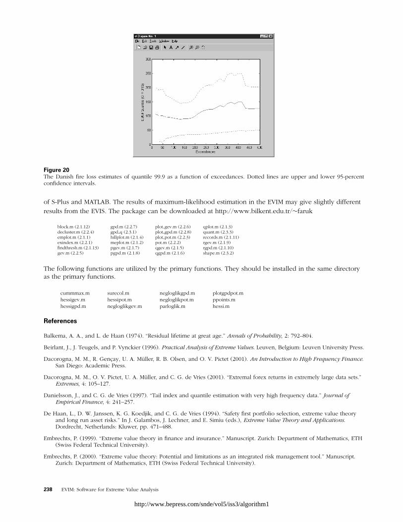
Figure 20The Danish fire loss estimates of quantile 99.9 as a function of exceedances. Dotted lines are upper and lower 95-percentconfidence intervals.

of S-Plus and MATLAB. The results of maximum-likelihood estimation in the EVIM may give slightly different

results from the EVIS. The package can be downloaded at http://www.bilkent.edu.tr/∼faruk

block.m (2.1.12) gpd.m (2.2.7) plot gev.m (2.2.6) qplot.m (2.1.3)decluster.m (2.2.4) gpd q (2.3.1) plot gpd.m (2.2.8) quant.m (2.3.3)emplot.m (2.1.1) hillplot.m (2.1.4) plot pot.m (2.2.3) records.m (2.1.11)exindex.m (2.2.1) meplot.m (2.1.2) pot.m (2.2.2) rgev.m (2.1.9)findthresh.m (2.1.13) pgev.m (2.1.7) qgev.m (2.1.5) rgpd.m (2.1.10)gev.m (2.2.5) pgpd.m (2.1.8) qgpd.m (2.1.6) shape.m (2.3.2)

The following functions are utilized by the primary functions. They should be installed in the same directoryas the primary functions.

cummmax.m surecol.m negloglikgpd.m plotgpdpot.mhessigev.m hessipot.m negloglikpot.m ppoints.mhessigpd.m negloglikgev.m parloglik.m hessi.m

References

Balkema, A. A., and L. de Haan (1974). “Residual lifetime at great age.” Annals of Probability, 2: 792–804.

Beirlant, J., J. Teugels, and P. Vynckier (1996). Practical Analysis of Extreme Values. Leuven, Belgium: Leuven University Press.

Dacorogna, M. M., R. Gencay, U. A. Muller, R. B. Olsen, and O. V. Pictet (2001). An Introduction to High Frequency Finance.San Diego: Academic Press.

Dacorogna, M. M., O. V. Pictet, U. A. Muller, and C. G. de Vries (2001). “Extremal forex returns in extremely large data sets.”Extremes, 4: 105–127.

Danielsson, J., and C. G. de Vries (1997). “Tail index and quantile estimation with very high frequency data.” Journal ofEmpirical Finance, 4: 241–257.

De Haan, L., D. W. Janssen, K. G. Koedjik, and C. G. de Vries (1994). “Safety first portfolio selection, extreme value theoryand long run asset risks.” In J. Galambos, J. Lechner, and E. Simiu (eds.), Extreme Value Theory and Applications.Dordrecht, Netherlands: Kluwer, pp. 471–488.

Embrechts, P. (1999). “Extreme value theory in finance and insurance.” Manuscript. Zurich: Department of Mathematics, ETH(Swiss Federal Technical University).

Embrechts, P. (2000). “Extreme value theory: Potential and limitations as an integrated risk management tool.” Manuscript.Zurich: Department of Mathematics, ETH (Swiss Federal Technical University).



Embrechts, P., C. Kluppelberg, and T. Mikosch (1997). Modeling Extremal Events for Insurance and Finance. Berlin: Springer.

Embrechts, P., S. I. Resnick, and G. Samorodnitsky (1998). “Extreme value theory as a risk management tool.” Manuscript.Zurich: Department of Mathematics, ETH (Swiss Federal Technical University).

Falk, M., J. Husler, and R. Reiss (1994). Laws of Small Numbers: Extremes and Rare Events. Basel, Switzerland: Birkhauser.

Fisher, R. A., and L. H. C. Tippett (1928). “Limiting forms of the frequency distribution of the largest or smallest member of asample.” Proceedings of the Cambridge Philosophical Society, 24: 180–190.

Ghose, D., and K. F. Kroner (1995). “The relationship between GARCH and symmetric stable processes: Finding the source offat tails in financial data.” Journal of Empirical Finance, 2: 225–251.

Gnedenko, B. (1943). “Sur la distribution limite du terme maximum d’une serie aleatoire” [On the distribution limit ofmaximum terms of risk series]. Annals of Mathematics, 44: 423–453.

Gumbel, E. (1958). Statistics of Extremes. New York: Columbia University Press.

Hauksson, H. A., M. Dacorogna, T. Domenig, U. Muller, and G. Samorodnitsky (2000). “Multivariate extremes, aggregation andrisk estimation.” Manuscript. Ithaca, NY: School of Operations Research and Industrial Engineering, Cornell University.

Hill, B. M. (1975). “A simple general approach to inference about the tail of a distribution.” Annals of Statistics, 3: 1163–1174.

Hols, M. C., and C. G. de Vries (1991). “The limiting distribution of extremal exchange rate returns.” Journal of AppliedEconometrics, 6: 287–302.

Hosking, J. R. M., and J. R. Wallis (1987). “Parameter and quantile estimation for the generalized Pareto distribution.”Technometrics, 29: 339–349.

Jansen, D., and C. G. de Vries (1991). “On the frequency of large stock returns: Putting booms and busts into perspective.”Review of Economics and Statistics, 73: 18–24.

Koedijk, K. G., M. M. A. Schafgans, and C. G. de Vries (1990). “The tail index of exchange rate returns.” Journal ofInternational Economics, 29: 93–108.

Longin, F. (1996). “The asymptotic distribution of extreme stock market returns.” Journal of Business, 63: 383–408.

Loretan, M., and P. C. B. Phillips (1994). “Testing the covariance stationarity of heavy-tailed time series.” Journal of EmpiricalFinance, 1: 211–248.

Mandelbrot, B. B. (1963). “The variation of certain speculative prices.” Journal of Business, 36: 394–419.

McNeil, A. J. (1997). “Estimating the tails of loss severity distributions using extreme value theory.” ASTIN Bulletin, 27:117–137.

McNeil, A. J. (1998). “Calculating quantile risk measures for financial time series using extreme value theory.” Manuscript.Zurich: Department of Mathematics, ETH (Swiss Federal Technical University).

McNeil, A. J. (1999). “Extreme value theory for risk managers.” In Internal Modeling and CAD II. London: Risk Books,pp. 93–113.

McNeil, A. J., and R. Frey (2000). “Estimation of tail-related risk measures for heteroscedastic financial time series: An extremevalue approach.” Journal of Empirical Finance, 7: 271–300.

Muller, U. A, M. M. Dacorogna, and O. V. Pictet (1996). “Heavy tails in high frequency financial data.” Discussion paper.Zurich: Olsen & Associates.

Muller, U. A., M. M. Dacorogna, and O. V. Pictet (1998). “Heavy tails in high-frequency financial data.” In R. J. Adler, R. E.Feldman, and M. S. Taqqu (eds.), A Practical Guide to Heavy Tails: Statistical Techniques and Applications. Boston:Birkhauser, pp. 55–77.

Pickands, J. (1975). Statistical inference using extreme order statistics. Annals of Statistics, 3: 119–131.

Pictet, O. V., M. M. Dacorogna, and U. A. Muller (1998). “Hill, bootstrap and jackknife estimators for heavy tails.” In R. J.Adler, R. E. Feldman, and M. S. Taqqu (eds.), A Practical Guide to Heavy Tails: Statistical Techniques. Boston:Birkhauser, pp. 283–310.

Reiss, R., and M. Thomas (1997). Statistical Analysis of Extreme Values. Basel, Switzerland: Birkhauser.



EVIM: A Software Package for Extreme Value Analysis in MATLABrgencay/evim.pdf · EVIM: A Software...

Documents

Transcript of EVIM: A Software Package for Extreme Value Analysis in MATLABrgencay/evim.pdf · EVIM: A Software...