EVIDENCE OF SALTWATER INTRUSION AT THE EMILY AND

EVIDENCE OF SALTWATER INTRUSION AT THE EMILY AND RICHARDSON PREYER BUCKRIDGE RESERVE,

TYRRELL COUNTY, NORTH CAROLINA

by Sharon Madden

Date: ______________ Approved: ___________________________________ Dr. James Pahl, Advisor _____________________________________ Dr. Dean Urban, Program Seminar Leader

Masters project submitted in partial fulfillment of the requirements for the Master of Environmental Management degree in

the Nicholas School of the Environment and Earth Sciences Duke University

2005

2

ABSTRACT

Saltwater intrusion caused by wind and storm events, rising sea-levels and human

construction of canal networks is a significant concern for coastal freshwater systems.

The Emily and Richardson Preyer Buckridge Coastal Reserve in Tyrrell County, NC was

purchased by the NC Division of Coastal Management with the objective of restoring

ditched wetland complexes - Peatland Chamaecyparis thyoides (L.) (Atlantic White

Cedar) Forests in particular. The canal network in the Reserve, which was built for cedar

harvest, flows into the Alligator River. It serves as a conduit for saltwater intrusion and

may be inhibiting regeneration of healthy C. thyoides.

The objective of this study is to determine the extent to which saltwater is

entering the peatland system through the canal network and moving laterally from the

canals into the peat soils. Hurricane Ophelia passed through on September 15, 2005

enabling study of storm event influences. Canal sampling stations and monitoring well

transects were set up to sample surface and pore water for specific conductivity, an

indirect measure of salinity, at distances from the outflow point to Alligator River from

September to November 2005. Changes in conductivity in canal stations across sampling

dates indicate the system response to Ophelia. Cation concentrations and soil samples

were analyzed from the transects to support evidence of saltwater intrusion and explore

trends between soils and levels of conductivity.

Saltwater was evident in the canal network at sampling stations and in the pore

water, as shown by high concentrations of K, Ca, Mg and Na. Ophelia pushed saltwater

deep into the canal network along the bottom of the canals. The saltwater was flushed

out slowly over the course of one to two months. In light of these trends, saltwater

intrusion must be addressed in restoration plans through the use of tide gates and long-

term management plans that address projected sea-level rise.

3

TABLE OF CONTENTS

LIST OF FIGURES ...................................................................................................... 4 LIST OF TABLES ........................................................................................................ 4 INTRODUCTION .........................................................................................................5 Objectives and Hypotheses .............................................................................................9 MATERIAL AND METHODS .....................................................................................10 Site Descriptions ............................................................................................................10 Transect Descriptions .....................................................................................................15 Sampling Methods .........................................................................................................16 Canal Surface Water .........................................................................................16 Porewater in Monitoring Wells ...........................................................................17 Soil Analyses from Monitoring Well Transects ....................................................18 Statistical Analyses .............................................................................................20 RESULTS .....................................................................................................................21 Environmental Conditions ...............................................................................................21 Canal Surface Water ......................................................................................................21 Pore Water in Monitoring Wells .....................................................................................25 Soil Analyses from Monitoring Well Transects ................................................................30 DISCUSSION .............................................................................................................33 Canal Surface Water .....................................................................................................33 Pore Water and Soils at Monitoring Well Transects .......................................................34 Restoration and Management Considerations .................................................................37 Tide Gates ........................................................................................................37 Sea-Level Rise .................................................................................................38 Further Research Opportunities ....................................................................................40 ACKNOWLEDGEMENTS …………………………………………………………42 REFERENCES ………………………………………………………………………43 APPENDIX I – RAW DATA ......................................................................................A1 APPENDIX II – SUMMARY STATISTICS ..............................................................A6 APPENDIX III – SAS CODE ....................................................................................A13

4

LIST OF FIGURES

1: Map of Coastal North Carolina ……………………………………………………….11 2: Map of the Buckridge Reserve …………………………………………………….….12 3: Map of Reserve roads and drainage network ……………………………………….…13 4: Map of Reserve natural communities ………………………………………………......14 5: Map of sampling stations and transects ………………………………………...……....17 6: Specific conductivity at sampling stations by depth and sampling date …….......………...23 7: Specific conductivity at transects by distance from edge ……………….....…………….26 8: Specific conductivity by depth to water table ………………………………………......27 9: Cation concentrations by transect and distance to edge …………………………....…...29 10: Specific conductivity by soil bulk density …………………………………………......31 11: Specific conductivity by percent soil organic matter ……………………………....…..32 12: Specific conductivity by soil carbon:nitrogen …………………………………….....…32 13: Map of lands close to sea level in Coastal North Carolina ……………………....…….40

LIST OF TABLES

1: Specific conductivity by sampling station, depth, sampling date …………………......….21 2: Mean conductivity at sampling stations …………………………………………...…...22 3: Specific conductivity by transect and distance from edge ………………………....…. .25 4: Correlation of cations in porewater …………………………………………….…….28 5: Cation concentration by transect and distance from edge ……………………...………28 6: Correlation of soil parameters ………………………………………………….……..30 7: Soil parameters by transect and distance to edge ………………………………..…….31

5

INTRODUCTION

Saltwater intrusion is the introduction of saltwater into freshwater systems. This

often occurs in coastal systems as a result of both natural and anthropogenic mechanisms.

Storm surges and strong wind events can push saltwater into freshwater channels, rising

sea levels will encroach on freshwater coastal systems and the construction of canals

provides a conduit through which saltwater can penetrate deep into a freshwater

environment. Saltwater can move into the freshwater system through both surface water

and groundwater connections to a saline source.

The extent of saltwater intrusion due to wind and storm events depends on wind

direction and speed, storm intensity, storm path and storm surge, which is directly related

to wind speed (Walker et al. 1987). The slope of the coastal shelf and orientation of the

shoreline will also dictate where and how much saltwater will enter the system from a

particular event. Hurricanes can be a significant mechanism of saltwater intrusion on the

Atlantic Coast from summer through fall. Freshwater coastal systems can be inundated

during hurricane events with saltwater that can seep into the groundwater (Anderson

2002).

Eustatic sea-level rise (SLR) is projected to be 1-2 mm/yr, which is the change in

sea level rise with a change in the ocean volume (Milly et al 2003). Rates of relative

SLR include the combination of eustatic SLR and local geologic conditions, such as local

elevation, subsidence and shoreline erosion. Relative sea-level rise for coastal North

Carolina is 3.3mm/yr as much of the land is below 1.5m in elevation (PSMSL 2003, Titus

and Richman 2001, Moorhead and Brinson 1995). Subsidence has been seen in coastal

peatland systems, such as in coastal Louisiana where relative SLR is 2.3mm/yr and

higher (Turner 1997, Day et al 2000). Rising sea levels will inundate shorelines and

promote saltwater intrusion into coastal freshwater systems; these coastal systems are at

high risk of loss to submergence with projected SLR.

Human creation of canals and ditches for drainage of freshwater systems

encourages saltwater intrusion where canals connect with a saltwater source (Craig et al

1979, Walker et al 1987, Turner 1997, Day et al 2000). Canals can carry saltwater deep

into coastal freshwater systems, especially as a result of wind and storm events. As canal

6

drainage will alter natural hydrology, reduced water tables provide an opportunity for

saltwater to seep out of canals through lateral subsurface flow and into porewater

(Barlow 2005). Canals greatly increase the extent to which saltwater can penetrate a

coastal freshwater system.

There are significant implications associated with saltwater intrusion on coastal

freshwater systems, peatlands in particular. The mortality of freshwater vegetation and

the shift in biogeochemical cycling from methanogenesis to sulfate reduction are the

primary consequences of saltwater intrusion that cumulatively result in collapse and

decomposition of peat soils, which in turn can result in loss of peatland systems.

Elevated salinity in the surface and pore water from saltwater intrusion can result

in mortality of freshwater vegetation. Many freshwater plant species are not adapted to

high salt levels and will not be able to survive. Living roots of freshwater plants are a

significant structural feature of peat soils and their death upon increased salinity will

result in collapse of these air-filled roots or, in other words, loss of turgor (DeLaune et al.

1994). With the loss of turgor of the complex root systems upon plant mortality, the peat

soils will collapse and decline in elevation. As the peat soil surface subsides, saltwater

can readily intrude into these now lower-lying areas and accelerate plant mortality and

loss of peatland systems.

Biogeochemical cycling within the peat soils is significantly altered with the

introduction of saltwater. Under natural freshwater conditions, methanogenesis is the

dominant method of anaerobic respiration in peatlands, resulting in production of

methane under these extremely reduced conditions (Mitsch and Gosselink 2000).

Saltwater introduces an abundant amount of sulfate, which shifts anaerobic respiration

from methanogenesis to sulfate reduction (Portnoy and Giblin 1997). Sulfate reduction is

more energetically favorable than methanogenesis and will increase oxidation of peat

soils (Mitsch and Gosselink 2000, Portnoy and Giblin 1997). As decomposition will thus

be accelerated, peat soils will collapse and decrease in elevation. This will also allow

saltwater to pond on the lowered peat surface, increasing sulfate inputs and exacerbating

peatland loss.

Saltwater intrusion is a large concern for much of the mainland coastal North

Carolina, as it is susceptible to storms and hurricanes during the summer and fall, low in

7

elevation with high relative SLR and networks of drainage canals cut across the

landscape. The Outer Banks run parallel to the mainland coastline and protect it from

direct influence of the Atlantic Ocean. The Albemarle and Pamlico Sounds are shallow

coastal inlets in eastern North Carolina that run between the Outer Banks and the

mainland. These sounds are estuarine systems, with seasonal variation in salinities where

high salinity is seen from September through November and lower salinity seen from

February through May (SAFMC 1998). Vertical stratification is homogeneous in the

Albermarle Sound where salinity is less than 5ppt (SAFMC 1998), while moderate

stratification is seen in the Pamlico Sound. Winds drive tides and water circulation in

the Albermarle Sound, suggesting that saltwater intrusion into the Albemarle-Pamlico

Peninsula will be influenced by strong wind and storm events.

The Albemarle Pamlico peninsula has the largest and deepest peat soils in North

Carolina as a result of the formation of the Coastal Plains over the last million years

(Ingram and Otte 1981). Fluctuations in sea level, with the expansion and contraction of

the polar ice caps, exposed and inundated the coastal plains creating scarps and sand

ridges (Daniel 1981). The withdrawal of the sea during the Wisconsin Ice Age (15,000

years ago) deeply downcut channels as much as 12 meters below present sea level (Heath

1975). As the sea level slowly rises, at about 0.3m per century since 1890 (Kaye and

Stuckey 1973), stream valleys were inundated and water tables rose, promoting peatland

formation (Daniel 1981). Peat formation in the Great Dismal Swamp and Albemarle-

Pamlico region began about 9,000 years ago when the sea level was about 130 feet below

present levels (Oaks and Coch 1973). Organic matter accumulated in the deep drainage

channels and depressions left after the last sea level retreat (Daniels 1981, Heath 1975).

Frequent precipitation and slow drainage maintained wetness in these areas, which

slowed decomposition, resulting in peat-based systems. The peat in the Great Dismal

Swamp is of fresh-water origin (Whitehead 1972), which is probably the case in the

Albermarle-Pamlico region (Heath 1975).

Much of coastal North Carolina has been ditched and drained for agriculture.

Richardson et al. (1981) estimated that 33% of the peatlands were fully converted with

another 36% partially converted as of 1979. With estimates of natural peatlands at 2.2

million acres, much of the peatlands have been altered. Drainage networks are typically

8

comprised of canals that are up to 3 to 4.5m deep, 4.5 to 7.6m wide at the top and spaced

about a 0.76 km apart with shallower, narrower ditches spaced frequently between canals

(Heath 1975). Drainage networks of peatlands close to the coastline flow into the Sounds

or estuarine river bodies that flow into the Sounds, providing an opportunity for saltwater

to move into the peatlands through the canals.

The viability of important and rare natural coastal communities is threatened by

the likelihood of saltwater intrusion into the coastal peatlands of North Carolina. Of

particular importance are the Peatland Atlantic White Cedar (Chamaecyparis thyoides

(L.), USDA Plant Database 2005) Forests. Harvesting, hydrological modification and

saltwater intrusion have caused a significant decline in these communities in both the

state of North Carolina and on a global scale (Schafale and Weakley 1990, Fuss 2001).

Pocosins and Carolina Bays are also natural peatland communities at risk of loss from

saltwater intrusion; these peatland types represent historic peat development though much

of them have been lost to ditching and drainage (Schafale and Weakley 1990).

The Division of Coastal Management purchased the Emily and Richardson Preyer

Buckridge Coastal Reserve with the objective of preserving and restoring these rare

natural communities, peatland Atlantic White Cedar forest in particular. Buckridge

Reserve is the largest largest and most inland coastal reserve at 18,652 acres located in

the Gum Neck Community of Tyrrell County, North Carolina. The largest contiguous

tract of regenerating Atlantic White Cedar (AWC) in North Carolina covers 4,000 acres

of the Reserve, while stressed and dead AWC stands are also present (Fuss 2001).

Harvesting practices, which began in the 1880’s and became more intensive from the

1950’s to the early 1980’s, have significantly modified the hydrology with the

construction of roads and a canal network. Canals and ditches can drain wetlands of both

surface and subsurface water and increase outflow rates (Gilliam and Skaggs 1981).

Roads can dam flow of surface and subsurface water, creating ponded conditions on one

side of the road (Mylecraine and Zimmermann 2000). As the canal network outflows to

Alligator River, which flows into the Albemarle Sound, there is an opportunity for

saltwater to enter the Reserve through the canals when pushed by wind tides and storm

events. AWC is tolerant of neither flooding nor saltwater (Mylecraine and Zimmerman

2000), thus successful regeneration will be hindered by present hydrologic conditions.

9

Preliminary monitoring has suggested that saltwater intrusion through the canal network

is stressing and killing AWC stands, preventing regeneration.

Salinity in the Alligator River averaged 3ppt during the study period from

September to November 2005, which is the period of highest salinities in the Albemarle

Sound (SAFMC 1998). Southwesterly winds push saltwater from the Albemarle Sound

into the Alligator River and into the canals at Buckridge Reserve. Hurricane Ophelia

brushed by this area, without making landfall, on September 15, 2005 as a Category 1

hurricane. This permitted analysis of the influence of a storm event on saltwater

intrusion into the canal network.

Objectives and Hypotheses

In light of the implications of saltwater intrusion on the peat soils and vegetation

at Buckridge Reserve, the purpose of this project was to determine if there is evidence of

saltwater intrusion and the extent to which it has entered the Reserve. This was studied

by looking at the surface water in the canals in a vertical profile, pore water in monitoring

wells and changes over time in response to Hurricane Ophelia.

There are four primary objectives of this study:

1. To determine the extent to which saltwater has moved into the Reserve along

the canal network.

2. To determine the extent to which saltwater has moved in the pore water

through the peat soils and to note respective water table and soil parameters

that may play a role in saltwater transmission.

3. To observe the influence of Hurricane Ophelia.

4. To provide restoration recommendations that address saltwater intrusion into

the Reserve and develop baseline data for further study.

10

My specific hypotheses are:

1. Presence of saltwater will decrease with increasing distance from the mouth of

the canal network to Alligator River.

2. Presence of saltwater will decrease with distance of the monitoring well

transect from the mouth of the canal network and also from the edge of each

transect.

3. Hurricane Ophelia will push saltwater through the canal network, increasing

levels at canal sampling stations.

METHODS AND MATERIALS

Site Description

Buckridge Coastal Reserve is located on the Albemarle Pamlico Peninsula in the

Gum Neck community of Tyrrell County, North Carolina (Figure 1). The Reserve is

bordered by the Gum Neck agricultural community to the west, the Alligator River to the

east and the south and the Frying Pan embayment to the north (Figure 2). The Gum Neck

agricultural community is bordered by a 2.5 to 3m high levee that is designed to protect

their farmlands from becoming flooded by Alligator River (Fuss 2001). The levee blocks

surface and subsurface water flow from the Gum Neck Drainage District through the

reserve, while agricultural drainage is pumped out at Cherry Ridge Landing. Figure 3

illustrates the road and canal network at the Reserve; roadside canals do not show up on

this figure. Thirty-one miles of road traverse the Reserve with canals running alongside

each road (ie. Juniper Rd. and Juniper Spur Rd. have canals running alongside them).

The canals range from 0.9 to 3m deep and 3 to 9.1m across, though are 1.8 to 2.4m deep

and 6 to 7.6m wide on average (Fuss 2001).

11

Figure 1. Map of Coastal North Carolina with Tyrrell County highlighted in pink and area of Buckridge Reserve outlined in blue box.

12

Figure 2. Map of the Emily and Richardson Preyer Buckridge Coastal Reserve, outlined in pink line, with study area outlined in green box. The yellow line marks a levee that borders the Gum Neck farming community and the orange circle indicates Cherry Ridge Landing, where water is pumped out of the farmland drainage network.

13

Figure 3. Map of roads (red lines) and drainage networks (blue lines) through Buckridge Reserve. (Source: Fuss 2001).

Peat depths in the Albemarle-Pamlico range from 0.3 to 2.4m, though can reach

up to 5.8m in relict channels (Ingram and Otte 1981). At the Reserve, peat depths are

known to range from 0.6 to over 2.7m (Fuss 2001). Logs and stumps of AWC and

cypress trees are typically found in the upper layers of the peat. With the variation in peat

topography, there are a variety of depressional and riverine wetland complexes and

natural communities. The wetland types at the Reserve consist of estuarine shrub scrub,

bottomland hardwood, riverine swamp forest, depressional swamp forest, hardwood flat,

Juniper Rd.

Grapevine Landing Rd.

Juniper Spur Rd.

14

pine flat and managed pineland (Fuss 2001). Natural communities found at the Reserve,

illustrated in Figure 4, are tidal cypress-gum swamp, tidal freshwater marsh, loblolly pine

(Pinus taeda L.), peatland AWC forest, non-riverine swamp forest and pond pine (Pinus

serotina Michx.) woodland (Fuss 2001).

Figure 4. Map of the natural communities found at Buckridge Reserve. (Source: Fuss 2001)

15

Transect site description

Figure 5 specifies the location of each of the four transects. The Shore transect

runs west from the shore of the Alligator River into the Reserve and represents the direct

influence of the river. The peat layer is thin at the edge of the shoreline and gets thicker

moving inland and is underlain with sand. Juncus roemerianus Scheele (Black

Needlerush) is found at the edge, with Liquidambar styraciflua L. (Sweet Gum),

Liriodendron tulipifera L. (Tulip Poplar), Platanus occidentalis L. (Sycamore), Quercus

phellos L. (Willow Oak), Acer rubrum L. (Red Maple) and Smilax spp. L. (Greenbrier)

along the transect. Phragmites australis (Cav.) Trin. Es Steud. (Common Reed)

dominates at 30m from the shore edge, at the end of the transect. All plant names are

from USDA-NRCS Plant Database (2005).

The Mouth transect is perpendicular to the Grapevine Landing Rd. canal, at 77m

from the point where the canal connects to the Alligator River. At 5m from the edge of

the transect, a swale enters the area that connects to the canal, closer to Alligator River.

The peat soils are thicker here than at the Shore Transect, and also underlain with sand at

depths below 1.2m. The soils were saturated throughout the study period and frequently

ponded, especially at the 5m well. Typha spp. L. (Cattail), Greenbrier, Red Maple,

Leucothoe racemosa (L.) Gray (Swamp dog-hobble), Sagittaria latifolia Willd.

(Broadleaf arrowhear), Arundinaria gigantea (Walt.) Muhl. (Giant Cane) and Carex spp.

L. (Sedges) are found throughout the transect. Cattail dominates the last 15m of the

transect.

The USGS transect runs perpendicular to the canal sampling station 7, which is

along Juniper Rd. and 2762m from the Alligator River along the canal network. The

transect begins near the road and runs through an area dominated by young trees such as

Red Maple and Pond Pine with Greenbrier and minimal understory. AWC was seen near

the transect, past the 30m well. The peat soils here are also deep, and saturated with

areas of ponding throughout the study period.

The Spur Rd. transect is located down the Juniper Spur Rd., across from canal

sampling station 10 at 4641m from the mouth of the canal network to Alligator River.

The transect begins near the road, where Common Reed dominates. The first 10m of the

transect is dominated by Cattail, Myrica cerifera (L.) Small (Wax-myrtle), Red Maple

16

and some Greenbrier and Broadleaf arrowhead. Woodwardia virginica (L.) Sm.

(Virginia chainfern) and Broadleaf arrowhead dominate beyond 15m from the edge of the

transect. Few AWC are seen near the 30m well. The peat soils here are very deep and

saturated, with Sphagnum spp. L. (Sphagnum mosses) accumulating on the peat surface.

Logs of cedar are found in the surface layers of the peat soils.

Sampling Methods

Canal Surface Water

Ten sampling stations were selected in the canal network starting from the

outflow point into Alligator River and along the Grapevine Landing Road canal and the

Juniper Road canal (Figure 5). Sampling stations were selected near well transects and at

points of connection with other canals. Specific conductivity at each of these sampling

stations was measured with a YSI Model 33 S-C-T meter (YSI Inc., Yellow Springs, OH,

USA) on six dates: September 6, September 23, October 1, October 15, October 28 and

November 11, 2005. Specific conductivity was used as an indirect measurement of

salinity due to the freshwater nature of the system and low salinities. Specific

conductivity is more sensitive to small changes in water chemistry than standard

measures of salinity such as with a refractometer, and measures the capacity of water to

conduct an electric current, which increases with concentration of dissolved salts,

measured in µmhos/cm (Hem 1985). Ranges of specific conductivity for freshwater are

from 0 to 1,300 µmhos/cm, for brackish water are 1,301 to 28,800 µmhos/cm and salty

water is greater than 28,800 µmhos/cm (Russell and Kane 2005).

To obtain a vertical profile of the surface water at the sampling station,

conductivity was measured in the middle of the canal at the surface and every 50

centimeters to the bottom of the canal. These measurements were conducted using either

a canoe, when launching the boat near the station was possible, or a long PVC pole, when

not, to reach out to the middle of the canal while standing on the road.

17

Figure 5. Map of canal sampling stations (blue) and monitoring well transects (red) (1998 imagery provided by NC Division of Coastal Management).

Pore Water in Monitoring Wells

Pore water was studied along the four transects described in the site description

section. At each transect, a monitoring well was placed at distances of 5, 15 and 30

meters from the shore, canal or road adjacent to a canal depending on the transect to find

gradients in conductivity and chemical components of the pore water along the transect

18

(Figure 5). The twelve PVC monitoring wells were 1.5 meters in length with 0.25mm

slotted well screen and were installed 1.2 meters deep in the peat soils on the 18th and 19th

of August 2005. As the peat layer is thinner at the transect along the shore, these wells

were only installed 0.3m deep. The wells were installed only as deep as the peat layer as

the study focuses on the effect of saltwater on the peat soils that characterize Buckridge

Coastal Reserve.

Wells were developed on September 5, 2005 by using a centrifugal, self priming

Masterflex L/S Sampling Pump (Cole-Parmer Instrument Company, Vernon Hills, IL,

USA) to pump out two volumes of well water or more until the water appeared clear of

any organic material. Wells were sampled on the same six dates as the canal stations:

September 6, September 23, October 1, October 15, October 28 and November 11, 2005.

During each visit, the water level in the well was measured and then the well was

pumped dry using a piston-driven self-priming hand pump. The wells were allowed to

recharge with water before conductivity was measured. Conductivity in the wells was

measured using the YSI Model 33 S-C-T meter at each well, though measurements at the

5 meter and 15 meter wells of the shore transect were often limited by shallow water

levels.

Pore water samples were taken on November 11, 2005 from all of the wells but

the 5 meter and 15 meter wells at the shore transect, which did not have sufficient water.

Duplicate samples of 50 mL were taken back to the lab to be analyzed for concentrations

of Na, Mg, K and Ca. Each sample was filtered with 25mm glass fiber syringe filters

with a GF/0.45 µm nylon membrane and acidified with 150 µL of 8N HNO3. Samples

were diluted 20-fold and analyzed for each cation using a Perkin-Elmer 5100PC Atomic

Absorption Spectrophotometer (Perkin-Elmer, Wellesley, MA, USA).

Soil Analyses from Monitoring Well Transects

Soil samples were taken on October 28, 2005 at two depths at each well except

for the 5 meter well at the shore transect which only had one sample due to the shallow

layer of peat. Samples were taken with a box corer (7.5 x 7.5 cm) in areas that had not

been walked on and as close to the well as possible. The box corer was pushed down

through the bare peat soil as deep as possible to obtain a sample reflective of the soil

19

through which the pore water in the well would pass. The samples represented the top 20

cm from the surface at the Shore, USGS and Spur Rd. transects and up to 50cm from the

surface at the Mouth transect. The lowest 20 cm of the sample were cut in half, making

samples of 562.5 cm3 in volume, then placed in a sealed plastic bag to be analyzed in the

lab. At the Spur Road and USGS transects, use of the box corer was made difficult by

logs and thick pieces of Atlantic White Cedar that had not fully decomposed. The one

sample at the 5 meter well at the shore transect was taken using a 7.5-cm diameter

aluminum corer, pushed into the peat layer to obtain a sample of the top 4.5cm of soil

that was 198.7 cm3 in volume.

In the lab the soils were analyzed for bulk density (43.3 Bulk Density and Total

Pore Space Carter 1993), percent organic matter (44.3 Ash Content and Organic Matter

Content, ASTM D2974 1988 Carter 1993) and total carbon and nitrogen (Total Carbon,

Hydrogen, and Nitrogen by Dry Combustion adapted from Black et al 1965). Soils were

prepared by removing live roots and pieces of cedar by hand, and then weighed in pre-

weighed aluminum foil containers. The soils were dried in a forced air oven at 105ºC for

five days. Once dried, the soils were reweighed. The volumes of the live roots and

pieces of cedar removed from the soil samples were determined by measuring the amount

of water they displaced when added to a graduated cylinder. Bulk density was then

calculated using the initial volume of the soil sample taken in the field, the volume of the

removed roots and cedar pieces and the dry weight of the soil according to Equation 1.

Eqn. 1. )()(

)(33 cmrootvolumecmsoilvolume

gdryweightyBulkdensit

−=

A subsample of the dry soil was then ground using a mortar and pestle and

shatterbox. For percent organic matter analysis, no more than 5 grams of each sample

was then added to pre-weighed crucibles for loss on ignition analysis. Crucibles with soil

were ashed in a muffle furnace at 500ºC for 4 hours and allowed to cool in a desiccator.

The remaining mineral soil was reweighed to determine the percent of organic matter lost

per sample.

20

Total carbon and nitrogen were analyzed by weighing no more than 10

micrograms of dried sample into pre-weighed tin capsules. These capsules were then dry

combusted on a Carlo Erba EA1112 CHN analyzer (ThermoQuest, Milan, Italy) to

determine the amount of carbon and nitrogen in each sample. The carbon and nitrogen

ratio was then calculated by dividing the percent carbon for each sample by the percent

nitrogen.

Statistical Analyses

All data analysis was performed using SAS for Windows Version 9.1 (SAS

Institute, Cary, NC, USA). Conductivity measurements for both canal surface water and

well pore water were normalized using a log10 transformation. The data for the canal

surface water was tested for differences between sampling stations, depths, sampling

stations by depth and these factors over sampling dates using a Repeated Measures

Analysis of Variances. Significant differences between each sampling station were tested

using a Tukey-Kramer Honestly Significant Difference (HSD) test.

Conductivity, water table, cation and soils data for the monitoring well transect

were treated as a factorial design experiment. A Factorial Analysis of Variance was used

to test for differences in conductivity between transect and between distances from the

edge and the interaction of transect and distance from the edge. Differences between

sampling dates, transects and distances from the edge, as well as any interaction between

these parameters, were tested through a Repeated Measures Analysis of Variance.

Significant differences between each transect, each distance from an edge and the

interaction of transect and distances from an edge were evaluated using a Tukey-Kramer

HSD test. This was repeated for log10-transformed cation concentration data and soil data

with a preliminary correlation analysis. The water table data was analyzed first using a

correlation analysis between depth to water table and the log10-transformed conductivity

data and followed by a Polynomial Regression analysis using a quadratic polynomial.

21

RESULTS

Environmental Conditions

Environmental conditions are from the Plymouth, NC Tidewater Research

Station, which is the nearest weather station at about 50 miles west of Buckridge Reserve.

Monthly average daily temperatures were 23.6ºC in September, 17.3ºC in October and

12.4º C in November 2005 (NC CRONOS 2005). Monthly precipitation averages were

63.8mm in September, 252.7mm in October and 64.5mm in November. Hurricane

Ophelia brushed by the Reserve on September 15 with sustained winds of up to 85 mph,

storm surges of 2 to 4 feet above tide levels and 6 to 8 feet at heads of bays and rivers,

and precipitation ranging from 4 to 9 inches (NCDC 2005). No other major storm events

occurred during the study period from September 6 through November 11.

Canal Surface Water

Specific conductivity between stations and across depths were not consistent

across sampling dates, as illustrated by the results of the Repeated Measures Analysis of

Variance in Table 1. Mean conductivity at each sampling station, averaged across

depths, is presented in Table 2 to illustrate differences between the stations. Figure 6

demonstrates the changes in conductivity at each measured depth over time at each

sampling station. Sampling stations further from the connection to Alligator River were

found to be lower in conductivity than those closer to the river.

Table 1. Repeated Measures ANOVA of specific conductivity by sampling station distance and depth, repeated over sampling dates (time).

Model Component Model DF Error DF F P

Station distance 9 15 10.29 <0.0001

Depth 1 15 7.14 0.0174

Depth*distance 9 15 1.7 0.1788

Time 5 75 67.74 <0.0001

Time*distance 45 75 5.86 <0.0001

Time*depth 5 75 2.53 <0.0001

Time*depth*distance 40 75 2.74 <0.0001

22

Table 2. Mean conductivity at each sampling station ± 1 SE. Values with the same letters are not significantly different (P>0.05) from each other.

Sampling Station Number

Distance from Alligator River

Average Specific Conductivity N

(meters) (µmhos/cm)

1 0 1925 ± 288.6a 17

2 77 1682 ± 210.7a 24

3 1492 1195 ± 172.7ab 30

4 1536 1433.3 ± 324.6a 12

5 1975 643.75 ± 39.62b 24

6 1982 720 ± 69.84b 30

7 2762 1121.4 ± 177.7b 35

8 3253 589.7 ± 28.7bc 29

9 3318 1197.2 ± 255.5a 18

19 4641 722.4 ± 42.6b 29

23

Figure 6. Graphs of specific conductivity at each sampling station by depth over sampling dates.

160

140

120

100

80

60

40

20

0

0 1000 2000 3000 4000D

epth

(cm

)Specific Conductivity (umhos/cm)

Sept 6

Sept 23

Oct 1

Oct 15

Oct 28

Nov 11

Sampling Station 1 (0m from mouth)

160

140

120

100

80

60

40

20

00 500 1000 1500 2000 2500 3000 3500 4000

Dep

th (c

m)

Specific Conductivity (umhos/cm)

Sept 6

Sept 23

Oct 1

Oct 15

Oct 28

Nov 11


200

180

160

140

120

100

80

60

40

20

00 500 1000 1500 2000 2500 3000 3500

Dep

th (

cm)


Sept 6

Sept 23

Oct 1

Oct 15

Oct 28

Nov 11


60

50

40

30

20

10

0

0 500 1000 1500 2000 2500 3000 3500

Dep

th (c

m)


Sept 6

Sept 23

Oct 1

Oct 15

Oct 28

Nov 11


160

140

120

100

80

60

40

20

00 200 400 600 800 1000 1200

Dep

th (c

m)


Sept 6

Sept 23

Oct 1

Oct 15

Oct 28

Nov 11


180

160

140

120

100

80

60

40

20

0

0 500 1000 1500 2000 2500

Dep

th (c

m)


Sept 6

Sept 23

Oct 1

Oct 15

Oct 28

Nov 11


24

Figure 6 (continued). Graphs of specific conductivity at each sampling station by depth over

sampling dates.

250

200

150

100

50

00 500 1000 1500 2000 2500 3000 3500 4000

Dep

th (

cm)


Sept 6

Sept 23

Oct 1

Oct 15

Oct 28

Nov 11


200

180

160

140

120

100

80

60

40

20

0

0 150 300 450 600 750 900

Dep

th (

cm)


Sept 6

Sept 23

Oct 1

Oct 15

Oct 28

Nov 11


80

70

60

50

40

30

20

10

00 500 1000 1500 2000 2500 3000 3500

Dep

th (

cm)


Sept 6

Sept 23

Oct 1

Oct 15

Oct 28

Nov 11


200

180

160

140

120

100

80

60

40

20

00 200 400 600 800 1000 1200

Dep

th (

cm)


Sept 6

Sept 23

Oct 1

Oct 15

Oct 28

Nov 11


25

Pore Water in Monitoring Wells

Conductivity in the pore water was found to be significantly different between

transects, between distances from an edge, and between wells within transects as

presented in Table 3. Figure 7 illustrates the conductivity for each transect by distance

from the edge. Mean conductivity was 1022.22 ± 77.8 µmhos/cm at the Spur Rd.

transect and 527.78 ± 33.63 µmhos/cm at the USGS transect and 3269.44 ± 211.6

µmhos/cm at the Mouth transect and 4291 ± 467.98 µmhos/cm at the Shore transect.

Averaged across transect, the mean conductivity was 2360.71 ± 445 µmhos/cm at 5

meters from an edge, 1776.19 ± 297.24 µmhos/cm at 15 meters from an edge and

2140.63 ± 352.33 µmhos/cm at 30 meters from an edge. The mean conductivity for each

transect is significantly different from each other with the highest mean conductivity at

the Shore transect, the next highest mean conductivity at the Mouth transect, then the

Spur Rd. transect and the lowest mean conductivity at the USGS transect. The P-value

for differences between mean conductivity is P<0.001 for both the Spur Rd. transect and

the USGS transect when compared with the each transect, while the P=0.0254 for

differences between the Mouth transect and the Shore transect. The mean conductivity

for each well can be found in Appendix II.

Table 3. ANOVA table for differences in specific conductivity between transect and distances from edge and their interaction.

Model Component Model DF Error DF F P

Model 7 58 103.28 <0.0001

Transect 3 58 48.86 <0.0001

Distance from edge 1 58 13.91 0.0004

Transect*distance 3 58 2.7 0.0540

26

Figure 7. Specific conductivity at each transect by distance of monitoring well from edge. Site*distance: P<0.0001.

F

F

F

F

F F

F

FF

F

F F

0

1000

2000

3000

4000

5000

6000

7000

8000

0 5 10 15 20 25 30

Spe

cific

Con

duct

ivity

(um

hos/

cm)

Distance from edge (m)

Spur Rd. Transect USGS Transect Mouth Transect F Shore Transect

Specific Conductivity at each monitoring well distance for each transect

There were no significant differences in conductivity across sampling date, as the results

of the Repeated Measures Analysis of Variance indicated. Conductivity stayed consistent

across transects (P=0.9375) and across distances (P=0.9995).

Conductivity and depth to water table were significantly correlated

(PCC=0.41655, P=0.0005, N=66). A quadratic relationship exists between depth to

water table and specific conductivity as results of a Polynomial Regression suggest

(P<0.0001, 2 and 63 df, F=15.56). Figure 8 illustrates the relationship between

conductivity and depth to water table, where conductivity increases with depth to water

table up to a point and then declines.

27

Figure 8. Specific conductivity and depth to water table with polynomial regression (f(x)= -0.818x^2 + 106.7x + 2044.1, r-square = 0.433)

0

1000

2000

3000

4000

5000

6000

7000

8000

-20 0 20 40 60 80 100 120 140

Spe

cific

Con

duct

ivity

(um

hos/

cm)

Depth to Water Table (cm)

Specific Conductivity by Depth to Water Table

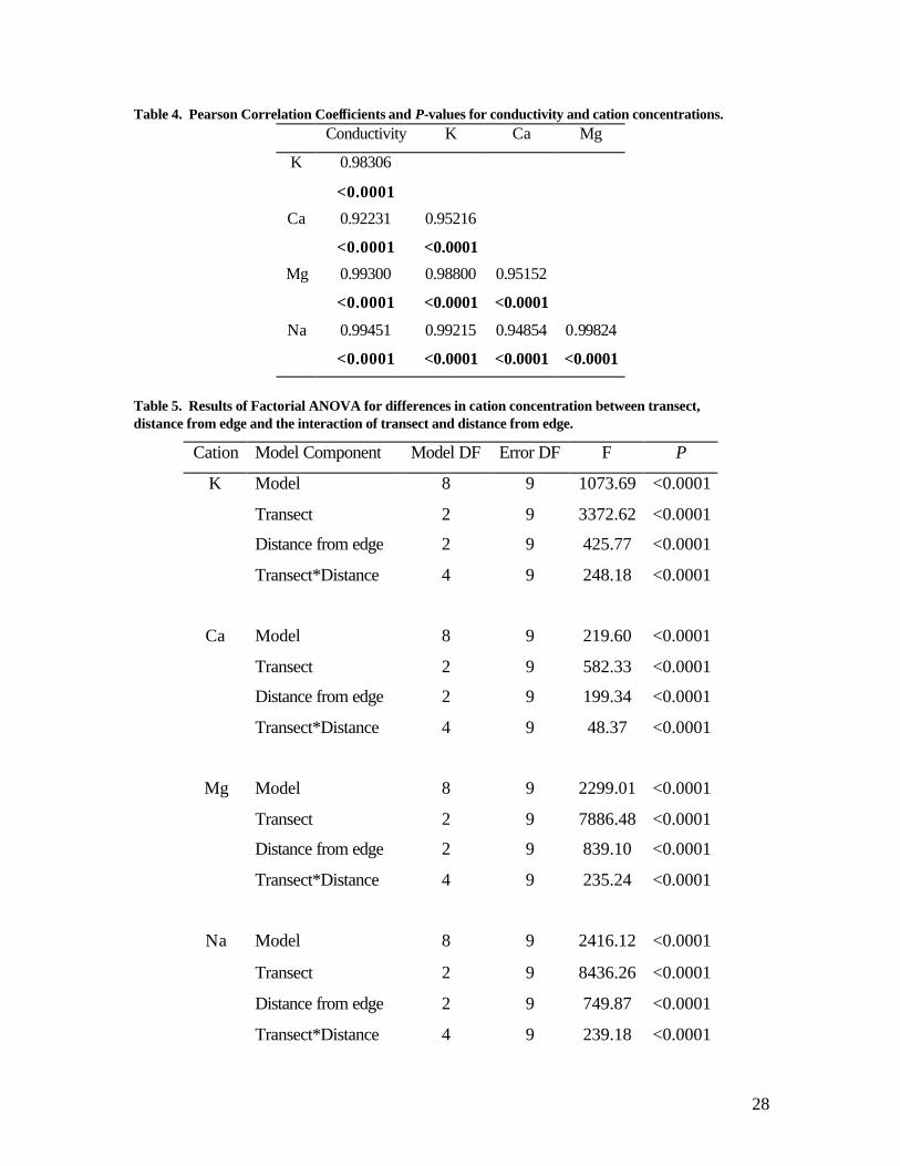
Potassium, calcium, magnesium and sodium cations were significantly correlated

with each other and with conductivity as seen in Table 4. There are significant

differences in all cation concentrations between transect and distance from the edge and

there is also differences between the cation concentrations between wells within each

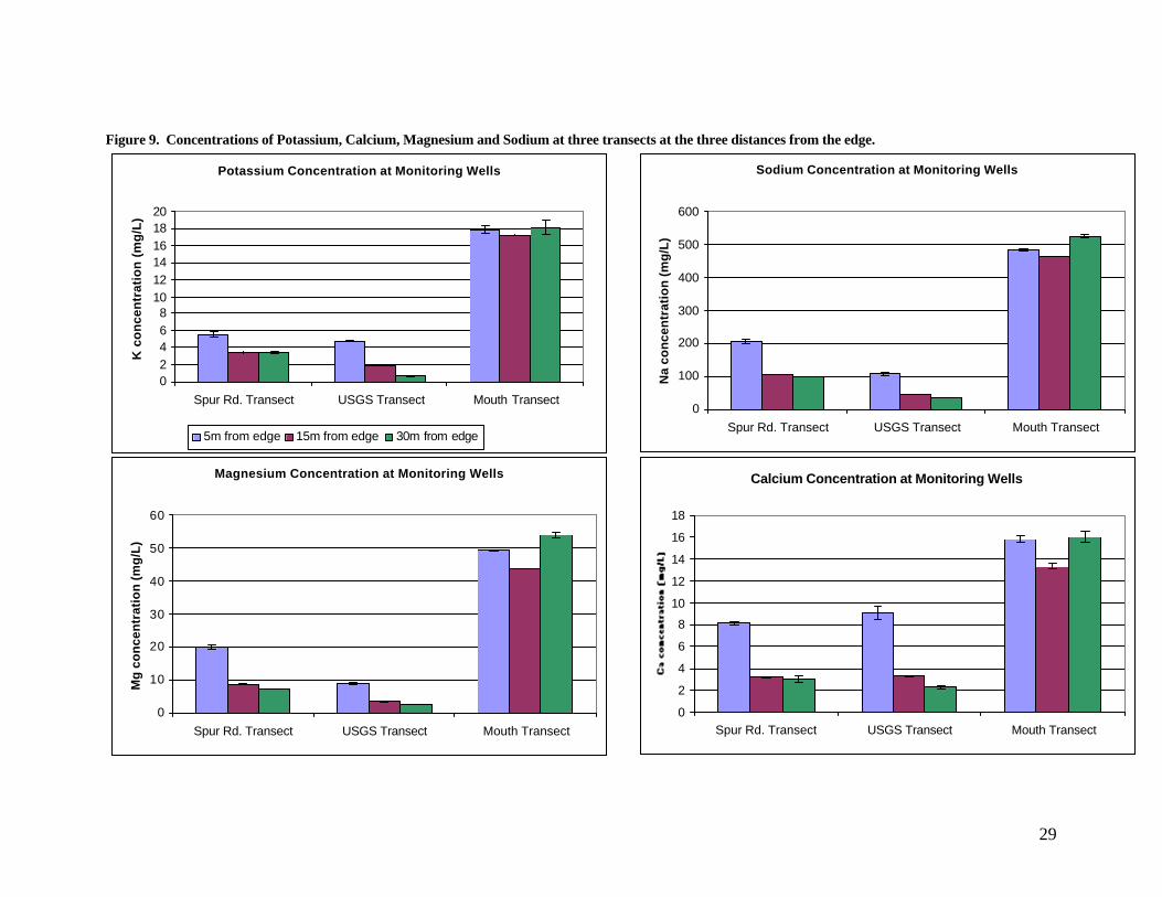
transect, as the results of the Factorial Analyses of Variance indicate in Table 5. Figure 9

illustrates the concentrations of each cation across transects. Cation concentrations are

the highest at the Mouth transect, where the same trend across distance from an edge is

seen of cations being higher at the 5m and 30m well than at the 15m well. The USGS

and Spur Rd. transects show decrease in cation concentration with distance from edge

though are significantly different for most of the cations. Similar concentrations of

calcium are seen between the Spur Rd. transect and the USGS transect.

28

Table 4. Pearson Correlation Coefficients and P-values for conductivity and cation concentrations. Conductivity K Ca Mg

K 0.98306

<0.0001

Ca 0.92231

<0.0001

0.95216

<0.0001

Mg 0.99300

<0.0001

0.98800

<0.0001

0.95152

<0.0001

Na 0.99451

<0.0001

0.99215

<0.0001

0.94854

<0.0001

0.99824

<0.0001

Table 5. Results of Factorial ANOVA for differences in cation concentration between transect, distance from edge and the interaction of transect and distance from edge.

Cation Model Component Model DF Error DF F P

Model 8 9 1073.69 <0.0001

Transect 2 9 3372.62 <0.0001

Distance from edge 2 9 425.77 <0.0001

K

Transect*Distance 4 9 248.18 <0.0001

Model 8 9 219.60 <0.0001

Transect 2 9 582.33 <0.0001


Ca


Model 8 9 2299.01 <0.0001

Transect 2 9 7886.48 <0.0001


Mg


Model 8 9 2416.12 <0.0001

Transect 2 9 8436.26 <0.0001


Na


29

Figure 9. Concentrations of Potassium, Calcium, Magnesium and Sodium at three transects at the three distances from the edge.

Potassium Concentration at Monitoring Wells

02468

101214161820

Spur Rd. Transect USGS Transect Mouth Transect

K c

on

cen

trat

ion

(m

g/L

)

5m from edge 15m from edge 30m from edge

Sodium Concentration at Monitoring Wells

0

100

200

300

400

500

600


Na

con

cen

trat

ion

(m

g/L

)

Calcium Concentration at Monitoring Wells

0

2

4

6

8

10

12

14

16

18


Magnesium Concentration at Monitoring Wells

0

10

20

30

40

50

60


Mg

co

nce

ntr

atio

n (

mg

/L)

30

Soil Analyses from Monitoring Well Transects

Correlation analyses indicate a significant correlation between all three soil

parameters, as shown in Table 6. There are significant differences in bulk density,

percent organic matter and C:N between transects, distances from an edge and within

transects, as indicated by the results the Factorial Analysis of Variance in Table 7.

However, within each model distance was not found to be significant and for bulk density

and C:N the interaction between transect and distance from an edge were also

insignificant. Nevertheless, each transect differs significantly in bulk density, percent

organic matter and C:N. Mean values of each soil parameter by distance were similar

between the Spur Rd. and USGS transects and between the Mouth and Shore transects.

The mean values for each soil parameter is presented in Appendix II.

Table 6. Pearson Correlation Coefficients and P-values for soil parameters.

While trends are apparent between specific conductivity and the three soil

parameters, cause and effect relationships cannot established due to the limited

knowledge of the hydraulic conductivity of these soils and the scope of this study. Figure

10 illustrates a decrease in conductivity with an increase in soil bulk density. Figure 11

shows an increase in conductivity with an increase in percent soil organic matter. Figure

12 also shows an increase in conductivity with an increase in C:N ratio.

Bulk Density Percent Organic Matter Carbon:Nitrogen

Bulk Density

-0.84100

<0.0001

-0.68230

0.0003

Percent Organic Matter

-0.84100

<0.0001

0.72142

0.0001

Carbon: Nitrogen

-0.68230

0.0003

0.72142

0.0001

31

Table 7. Results of Factorial ANOVA for each soil parameter. Significant P-values in bold.

0

1000

2000

3000

4000

5000

6000

7000

0 0.2 0.4 0.6 0.8 1 1.2

Spe

cific

Con

duct

ivity

(um

hos/

cm)

Bulk Density (g/cm^3)

Specific Conductivity by Bulk Density

Figure 10. Specific conducitivity by bulk density of peat soils (Pearson Correlation Coefficient [PCC]=0.69062, P <0.0001).

Soil Parameter Model Component Model DF Error DF F P

Model 11 11 5.67 0.0039

Transect 3 11 14.38 0.0004


Bulk Density

Transect*Distance 6 11 2.43 0.0959

Model 11 11 60.9 <0.0001

Transect 3 11 199.9 <0.0001


Percent

Organic

Matter


Model 11 11 3.91 0.0164

Transect 3 11 10.01 0.0018


C:N


32

0

1000

2000

3000

4000

5000

6000

7000

0 10 20 30 40 50 60 70 80 90 100

Spe

cific

Con

duct

ivity

(um

hos/

cm)

Percent Organic Matter

Specific Conductivity by Percent Soil Organic Matter

Figure 11. Specific conductivity by percent soil organic matter of peat soils (PCC=-0.93619, P<0.0001).

0

1000

2000

3000

4000

5000

6000

7000

0 5 10 15 20 25 30 35

Spe

cific

Con

duct

ivity

(um

hos/

cm)

C:N ratio

Specific Conductivity by Carbon:Nitrogen Ratio

Figure 12. Specific conductivity by carbon:nitrogen ratio of peat soils (PCC=-0.68175, P=0.0003).

33

DISCUSSION

Canal Surface Water

Sampling of canal surface water illustrated that, in general, conductivity

decreased with distance from the outflow point to Alligator River, and thus confirmed my

hypothesis that the canal network allowed saline water from Alligator River to intrude

into the Reserve. A closer look at the results of the conductivity against distance from

mouth and vertical depth test as they pertain to the spatial distribution of sampling

stations indicate interesting patterns. There are significant differences in mean

conductivity between sampling stations 1 and 2 (mouth and 77m from mouth) and

stations 5, 6, 7, 8 and 10 (1975m, 1982m, 2762m and 4641m respectively. However,

sampling station 9, which is one of the farthest stations at 3318m from the mouth, is not

significantly different from stations 1 and 2. Measurements at sampling station 9 for

each sampling date and personal observations at all sampling stations suggest that the

influence of Hurricane Ophelia lasted for a longer period as movement of water from this

point in the canal appeared slower than at the rest of the sampling stations. Before the

hurricane event, conductivity measured around 500 µmhos/cm across vertical depth,

meaning the surface water at this station was well-mixed and low in conductivity. After

the hurricane event, conductivity jumped to 3500 µmhos/cm at the surface and 3400

µmhos/cm at the bottom of the canal station. While the water at the surface returned to

lower conductance levels (400 µmhos/cm) after about 3 weeks, conductance at the

bottom of the canal dropped to 600 µmhos/cm after 5 weeks. This suggests that the slow

flushing of higher conductance water pushed in from the hurricane results in a high mean

conductivity for this sampling station during the sampling period. Additional sampling

days may actually show that conductivity is low at this station in the absence of

significant storm and wind events, such as a hurricane.

While conductivity returned to pre-hurricane levels after 3 weeks, a wedge with

increasing conductivity near the bottom of the canal station was common throughout yet

most significant at sampling station 7 (2762m). Two types of mixing can explain this

phenomena: salt-wedge and partial mixing (Mann 2000). Where there is a distinct

boundary between the freshwater upper layer and higher conductivity lower layer, mixing

34

is minimal with a sharp transition between layers, called a salt-wedge. This is seen as

sampling stations 7 where water at the surface of increased from 400 µmhos/cm to 700

µmhos/cm after the hurricane and dropped to 500 µmhos/cm after 3 weeks, while below

100cm from the surface, the conductivity increases from 400 µmhos/cm before the

hurricane to a maximum of 3900 µmhos/cm after the hurricane (Figure 6). The sampling

stations that also illustrate a gradient from low to high conductivity with depth are more

reflective of partial mixing, which is caused by tides or winds. This can be seen at

sampling station 3 and 6 (Figure 6). The difference in mixing between sampling station 3

and 6 versus sampling station 7 can be attributed to proximity to the mouth, where

stations 3 and 6 are more heavily influenced by wind tides. The common trend between

these stations suggests higher conductivity water moves into the ditch network along the

bottom of the canals. USGS preliminary data also showed this trend (Strickland 2005) at

two of their canal monitoring stations further inland. Conductivities were higher at the

bottom of the canals after the hurricane but returned to the lower levels seen at the

surface 3 weeks later.

These results indicate the importance of freshwater discharge and precipitation in

flushing saltwater from the Reserve. Saltwater intrusion was evident across sampling

stations, mainly entering the systems at the bottom of the canals though seen across the

vertical profile in sampling stations 4, 5 and 9. The saltwater was slowly flushed from

the system over time with freshwater discharge and precipitation events. Saltwater found

near the surface flushed quickly, while saltwater wedges were flushed anywhere from

one to two months after the hurricane. The nature of freshwater discharge from the

system prevents saltwater from remaining in the canals for extended periods of time,

though the seasonal fluctuations in salinity (SAFMC 1998), wind events and storm events

may illustrate different trends during other parts of the year.

Pore Water and Soils at Monitoring Well Transects

Conductivity in pore water illustrates similar trends between transects as seen at

canal sampling stations. The Shore and Mouth transects were significantly different from

each other as well as the farther inland USGS and Spur Rd. transects, which were not

significantly different. Furthermore, significant differences between distances of

35

monitoring wells from an edge showed a general decrease in conductivity as distance

from an edge increased. The distance from a surface water source of salinity is an

important variable in predicting conductivity in pore water (Hackney and de la Cruz

1978). Cation concentrations were also reflective of this pattern, where highest

concentrations were seen at the Mouth transect and at distances closer to an edge. These

trends suggest movement of water from the canals through the peat soils that result in

high conductivity in the pore water. However, the significant interaction between

transect and distance from an edge requires a closer look at each transect.

The Spur Rd. transect is the farthest along the ditch network, though conductivity

levels are higher than that of the USGS transect. Mean potassium, magnesium and

sodium cation concentrations are significantly higher at the Spur Rd. transect than at the

USGS transect. While conductivity and cation concentration decreases with distance

from the edge, the corresponding mean conductivity of the canal sampling station (10)

across from this transect is lower than that of the pore water. The cause of this increase

may be due to an unknown hydrologic connection to Alligator River, as the mapped end

of this canal is about 500 meters from the river and the wells are about 600 meters from

the river. Perhaps a storm surge or strong wind event pushed water from the river into

the canal or peat soils near this transect allowing infiltration of salts into the peat soils as

suggested by Anderson (2002). As there was no significant difference between sampling

dates to attribute this to Hurricane Ophelia in particular, further reconnaissance is

necessary to uncover speculated hydrologic connections with the Alligator River and

possible past overwash events.

The USGS transect fits the hypothesized model, where conductivity decreases

with distance from the edge and mean conductivity for the transect is lower than those

closer to the Alligator River. Concentrations of all four cations also decrease with

distance from the edge and are the lowest concentrations among the transects sampled.

The mean conductivity of the surface water at sampling station 7, across from this

transect, is higher than the mean conductivity of the pore water. This suggests that water

movement through the soil from the canal was limited, perhaps due to soil characteristics.

The Mouth transect showed high conductivity levels, though lower than the Shore

transect. Changes in conductivity with distance from the canal along this transect did not

36

show the same pattern as seen at the other transects. Mean conductivity at the well 30m

from the canal was higher than that of the 15 and 5m wells. The low-lying

microtopography at this transect may be the cause of this trend. A depression, or swale,

that connects with the canal closer to the mouth runs through the transect at the 5m well.

Strong winds can push saltwater from the canal up through the swale and across this low-

lying area, leaving salts behind. Conductivity may be higher at the 5m and 30m wells as

these areas were observed to be lower than at the 15m well, permitting longer periods

ponding and infiltration of saltwater. Concentrations of all four cations reflect the trends

seen in conductivity measurements, again supporting the influence of saltwater.

The Shore transect had the highest conductivity levels as it is directly influenced

by the Alligator River. Conductivity was highest at the well 5m from the river and

decreased at the 15m well but slightly increased at the 30m well. The slight difference

between the 15m and 30m wells could be an artifact of the few sampling measurements

at the 15m well due to low water tables.

Water table measurements and specific conductivity illustrated dilution effects as

conductivity measurements were low with high water tables. These effects were seen up

to water table depths of 60cm from the surface, when deeper water tables actually

showed lower conductivity. This drop in conductivity with deeper water table depths

could be due to the decrease in influence of saltwater on subsurface water chemistry or an

isolation of the groundwater from saltwater sources. The deepest water tables where seen

at the wells on the Shore transect, which may indicate minimal transmission of saltwater

through the deeper peat soils in this area.

The significant differences in the soil parameters between the transects indicate

trends in soil parameters and specific conductivity by transect. The shore transect has

high bulk density and the lowest percent soil organic matter and carbon to nitrogen ratio.

This may suggest influence of shoreline erosion and/or oxidation and decomposition

from biogeochemical shifts to sulfate reduction as sulfates are introduced by the saltwater

(Portnoy and Giblin 1997). As transects further inland from the Alligator River decrease

in bulk density and increase in percent soil organic matter and carbon to nitrogen ratios,

the possibility of saltwater intrusion promoting decomposition at the Shore transect and

to lesser extent at the Mouth transect is reasonable. The increase in carbon to nitrogen

37

ratios father inland are due to large increases in carbon, though small increases in

nitrogen were also seen. It must also be noted that peat depths are shallower at the Shore

transect and become increasingly greater from the Mouth transect to the USGS transect

with the deepest peats at the Spur Rd. transect.

Restoration and management considerations

Evidence of saltwater intrusion in the surface water of the canal network and the

pore water of the peat soils requires appropriate restoration measures. Restoration goals

are to be based on rehabilitating conditions that have been impacted by the construction

of the road and canal network. While installation of tide gates can prevent saltwater

intrusion into the canal network, the impact of future projections of SLR must be

considered.

Tide Gates

Tide gates are culverts placed in canals and ditches with a movable flap gate that

open and close in response to water levels (Giannico and Souder 2004). The gates will

open as tides are going out to allow outflow of freshwater and will close when tides are

coming in to prevent inflow of saltwater. Installation of the tide gates is recommended at

the mouth of the canal network into the Alligator River. This is the direct source of

saltwater and conductivity measurements were elevated in the adjacent peat soils. It

would be best to install them as close to the river as possible to prevent intrusion into

unrecognized swales, such as the one seen to penetrate the Mouth transect.

As one of the objectives of restoration is to promote regeneration of AWC,

location of tide gates further inland to protect waters feeding into regenerating AWC

areas is another option. Figure 4 shows a large stand of healthy regenerating AWC along

the Spur Rd. and Juniper Rd. heading East. A saltwater wedge was seen along the

adjacent canal after Hurricane Ophelia. Placement of a tide gate near the mouth will

prevent saltwater from entering the canals that connect to these regenerating stands. This

will also protect the area further west on Grapevine Landing Rd. near Sampling Station 9,

where a significant jump in conductivity was seen after Hurricane Ophelia.

38

There may be additional hydrologic connections to the Alligator River that this

study did not capture. Canals and ditches run through the southern part of the reserve and

connect with Alligator River at the southern Reserve border. Sampling station 4 was

located in one of the canals that have a southern connection. Mean conductivity as seen

in Table 1 is higher at this station than at Sampling Station 3, which is located directly

across from this station but in the main Grapevine Landing canal. Given that my study

has indicated the potential for saltwater intrusion into the interior areas of the Reserve

through the canal network, it is reasonable to expect that saltwater could be pushed up

from the south through this canal during storm and wind events that can feed into the

northern parts of the reserve. Entrance of saltwater at the southern part of the Reserve is

a large concern as there are stands of mature and healthy regenerating AWC. There is

also a connection with the Frying Pan Embayment at the northern part of the Reserve,

which may also be a source of saltwater as it connects with the Alligator River and is

closer to the Albemarle Sound. There are large tracts of regenerating AWC in this area

as well. Further research is needed in both the northern and southern parts of the reserve.

Sea-Level Rise

Sea-level is projected to rise at a rate of 1-2 mm/yr globally and up to 3.3mm/yr

in coastal North Carolina (Milly et al 2003, Titus and Richman 2001, Moorhead and

Brinson 1995). Projected climate change will increase SLR resulting in a eustatic rise of

48cm by the year 2100 (Houghton et al 2001). With the additional impact of climate

change, relative SLR near Buckridge Reserve can be around 70 to 75cm by 2100. This

will increase saltwater intrusion into the reserve and raise serious concerns for the future

of Buckridge Reserve.

Raised sea levels will submerge much of the low-lying coastal reserve and

increase the saltwater intrusion through the canal network. Saltwater may penetrate

deeper inland as tidal influence can become more significant and the mouth of the canal

network at a point further inland along the canal. Though I am uncertain about the

amount of freshwater discharge necessary to push out the saltwater we have seen during

this study, it is possible that the volume of freshwater discharge leaving the reserve may

not be enough to counter this saltwater intrusion. It took up to two months to flush

39

saltwater from Hurricane Ophelia, which was a single saltwater intrusion event, which

implies that consistent intrusion from raised sea levels may result in an overall increase in

the salinity of the canal water. It must be considered, however, that this was a drought

year, implying that saltwater may be flushed out faster under normal weather conditions.

I expect rainfall to be most heaviest during the spring, when the system would be most

resilient to saltwater intrusion as flushing would be at its peak.

With the potential of increased salinity and submergence of these peatlands by

SLR, comes impacts to the stability of the peatland communities. As saltwater moves

through the surface and porewater, mortality of freshwater vegetation will increase and

result in the collapse of peat soils (DeLaune 1994). Also, introduction of sulfates in the

saltwater will promote sulfate reduction over methanogenesis, which increases peat

oxidation and results in leaching of nutrients that are released during decomposition

(Portnoy and Giblin 1997, Gauci et al 2004, Vile et al 2003). Subsidence will occur

from both of these processes, which will lower the peat surface, allowing for even more

saltwater inundation, which will accelerate the loss of these coastal peatland systems.

The topography of Buckridge Reserve and the Albemarle Pamlico peninsula as a

whole is very flat, with virtually no slopes. A significant rise in sea-level to land

elevation will inundate a large portion of the Reserve and the peninsula as shown in

Figure 13. Because of the low-lying flat land, there is not an opportunity for the coastal

freshwater wetland communities at Buckridge to migrate upland (Moorhead and Brinson

1995). With slopes sufficient for vertical migration being greater than 2000m inland,

much of the area will become salinized, preventing re-establishment of the freshwater

vegetation. Also, the nature of peatland establishment at the Reserve and on the

peninsula, was not due to sediment accumulation but a result of several thousands of

years of peat accretion. Peat accretion at the project sea-level will not be rapid enough

for peatlands to migrate with the rate of SLR. Moorhead and Brinson (1995) predict that

this area will be converted to open water by the year 2100, which is a result of the flat

topography, peat subsidence due to saltwater intrusion and the rapid rate of SLR.

Restoration efforts must consider the loss of this coastal peatland to projected

SLR. While it is hard to mitigate, tide gates are a precursory step to prevent saltwater

intrusion with rising sea levels in the immediate future. It is also recommended to focus

40

regeneration efforts on AWC stands that are further inland. As saltwater intrusion across

the peat surface or in the subsurface water is already speculated near the Spur Rd.

transect, which is 500m from the Alligator River, SLR is a serious concern as it will

increase the area of influence of saltwater intrusion. Long-term planning and adaptive

management must be involved in the restoration plan for the Reserve.

Figure 13. Lands close to sea level (Source: Titus and Richman 2001)

Further Research Opportunities

This study provides baseline data for further monitoring and additional research.

As the study period only lasted from September to mid-November, I recommend that

sampling continues throughout the year and for additional years to capture seasonal

trends, additional storm events and yearly variation. SAFMC (1998) noted that salinities

below 1.5 m

1.5–3.5 m

above 3.5 m

30 miles

41

do vary between seasons, with the highest salinities seen at the same time of year as this

study. Lower salinities may be seen in the spring months due to flushing of freshwater

out of the Reserve with increased precipitation events.

Using similar methods of canal sampling stations and monitoring well transects,

the southern part of the Reserve should be studied. There is an important opportunity

here as this is where one of the very few mature stands of AWC is located. While less is

known about the extent of the canal and ditch network in this area due to access

limitations, gaining access to survey functional canals and ditches and their possible

connections is a first step.

Additional hydrologic studies should include creating a water budget to

determine discharges and water inputs to the system. Water quality studies should be

incorporated to determine if there are nutrient losses due to peat oxidation, which has

been found in other Coastal North Carolina peatlands (Richardson 1981, Gilliam and

Skaggs 1981), and if mercury, which binds strongly to organic matter, has been released

(Andriesse 1988). Nutrients and mercury in drainage waters can have serious

downstream water quality impacts, such as eutrophication and toxic mercury effects on

fish and wildlife.

Buckridge Reserve serves as an excellent research opportunity to learn more

about coastal peatland systems in North Carolina and the effects of saltwater intrusion.

As much of the coastal peatlands have been drained, restoration efforts are important not

only to restore natural communities but to gain understanding and set an example of how

to deal with natural and anthropogenic causes of saltwater intrusion.

42

ACKNOWLEDGEMENTS

I wish to thank my MP advisor, Dr. James Pahl, for all of us help in setting up this project

and guiding me through all of the steps to prepare this project report. I would also like to

thank Melissa Carle, my supervisor at NC Division of Coastal Management for providing

me the opportunity to work on this project at the Emily and Richardson Preyer Buckridge

Coastal Reserve and lending her support. Guy Stefanksi, Woody Webster, Jennifer

Rouse and Sean McGuire of NC DCM helped in the field and with the mapping

components of the project. Kristin Knight and Andy Sartor also helped greatly in the

field and provided support. Wes Willis, Paul Heine and Brian Roberts assisted with lab

work. I would also like to thank my family and friends for providing never-ending

support throughout my graduate career. This project was funded by the Duke University

Wetland Center and a Clean Water Management Trust Fund grant awarded to the

Division of Coastal Management.

43

REFERENCES Anderson, W.P. 2002. Aquifer salinization from storm overwash. Journal of Coastal

Research 18(3):413-420. Andriesse, J.P. 1988. Nature and management of tropical peat soils. Soil Resources,

Management and Conservation Service, FAO Land and Water Development Division, FAO Soils Bulletin No. 59.

Barlow, P.M. 2005. Ground water in freshwater-saltwater environments of the Atlantic

Coast. US Geological Survey, Circular 1262. Carter, M.R.(ed) 1993. Soil Sampling and Methods of Analysis. pp 449-450. Canadian

Society of Soil Science. Lewis Publishers, Boca Raton, FL. Day, J.W., L.D. Britsch, S.R. Hawes, G.P. Shaffer, D.J. Reed, D. Cahoon. 2000. Pattern

and process of land loss in the Mississippi Delta: spatial and temporal analysis of wetland habitat change. Estuaries 23(4): 425-438.

DeLaune, R.D., J.A. Nyman and W.H. Patrick, Jr. 1994. Peat collapse, ponding and

wetland loss in a rapidly submerging coastal marsh. Journal of Coastal Research 10(4): 1021-1030.

Douglas, B.C. and W.R. Peltier. 2002. The puzzle of global sea – level rise. Physics

Today 55(3):35-40. Fuss, J.D. 2001. Restoration and management plan for the Emily and Richardson Preyer

Buckridge Coastal Reserve, Tyrrell County, North Carolina: a conceptual approach. North Carolina Coastal Reserve Program, Division of Coastal Management, Department of Environment and Natural Resources, Raleigh, NC.

Gauci, V., E. Matthews, N.Dise, B. Walter, D. Koch, G. Granberg, and M. Vile. 2004.

Sulfur pollution suppression of the wetland methane source in the 20th and 21st centuries. Proceedings of the National Academy of Sciences 101(34): 12583-12587.

Giannico, G.R. and J.A. Souder. 2004. The effects of tide gates on estuarine habitats and

migratory fish. Oregon State University, Oregon Sea Grant Publication ORESU-G-04-002.

Gilliam, J.W. and R.W. Skaggs. 1981. Drainage and agricultural development: effects

on drainage waters. Pp. 109-124 in C.J. Richardson (ed.). Pocosin wetlands: an integrated analysis of Coastal Plain freshwater bogs in North Carolina. Hutchinson Ross: Stroudsbourg, Pennsylvania.

44

Hackney, C.T. and A.A. de la Cruz. 1978. Changes in interstitial water salinity of a Mississippi tidal marsh. Estuaries 1(3): 185-188.

Heath, R.C. 1975. Hydrology of the Albemarle-Pamlico region North Carolina: a

preliminary report of the impact of agricultural developments. U.S. Geological Survey Water Resources Investigations 9-75, in cooperation with N.C. Department of Natural and Economic Resources, Raleigh, North Carolina.

Hem, J.D. 1985. Study and interpretation of the chemical characteristics of natural

water. U.S. Geological Survey, Water Supply Paper 2254. Houghton, J.T., Y. Ding, D.J. Griggs, M. Noguer, P.J. van der Linden, X. Dai, K.

Maskell and C.A. Johnson. 2001. Climate Change 2001: The Scientific Basis. Intergovernmental Panel on Climate Change, Third Assessment Report.

Ingram, R.L. and L.J. Otte. 1981. Peat in North Carolina wetlands. Pp. 125-134 in C.J.

Richardson (ed.). Pocosin wetlands: an integrated analysis of Coastal Plain freshwater bogs in North Carolina. Hutchinson Ross: Stroudsbourg, Pennsylvania.

Mann, K.H. 2000. Ecology of Coastal Waters with Implications for Management,

Second Edition. Blackwell Science, Inc., Malden, Massachusetts. Milly, P.C.D., A. Cazenave, and M.C. Gennero. 2003. Contribution of climate-driven

change in continental water storage to recent sea-level rise. Proceedings of the National Academy of Sciences of the United States of America 100(23):13158-13161.

Moorhead, K.K. and M.M. Brinson. 1995. Response of wetlands to rising sea level in

the lower Coastal Plain of North Carolina. Ecological Applications 5(1): 261-271.

Mylecraine, K. and G. Zimmerman. 2000. Atlantic white cedar: ecology and best

management practices manual. Department of Environmental Protection, Division of Parks and Forestry, New Jersey Forest Service, Trenton, New Jersey.

National Climatic Data Center. Hurricane Ophelia: Event Record Details.

http://www4.ncdc.noaa.gov/cgi-win/wwcgi.dll?wwevent~ShowEvent~590780, last accessed December 13, 2005.

North Carolina Climate Retrieval and Observations Network Of the Southeast Database.

2005. Plymouth Tidewater Research Station. State Climate Center of North Carolina. http://www.nc-climate.ncsu.edu/cronos/index.php?station=PLYM&temporal=M, last accessed December 14, 2005.

45

Portnoy, J.W. and A.E. Giblin. 1997. Biogeochemical effects of seawater restoration to diked salt marshes. Ecological Applications 7(3): 1054-1063.

PSMSL. 2003. Permanent Service for Mean Sea Level Website, last accessed October

2005. Richardson, C.J., R. Evans, and D. Carr. 1981. Pocosins: an ecosystem in transition. Pp

3-19 in C.J. Richardson (ed.). Pocosin wetlands: an integrated analysis of Coastal Plain freshwater bogs in North Carolina. Hutchinson Ross: Stroudsbourg, Pennsylvania.

Russell, G.M. and R.L. Kane. 2005. Bathymetry, freshwater flow, and specific

conductance of Matlacha Pass, Southwestern Florida. U.S. Geological Survey, South Florida Information Access, Water-Resources Investigations Report 93-4057. http://sofia.usgs.gov/publications/wri/93-4057/specificc.html, last accessed December 3, 2005.

Schafale, M.P. and A.S. Weakley. 1990. Classification of the natural communities of

North Carolina: 3rd approximation. N.C. Department of Environment, Health, and Natural Resources, Division of Parks and Recreation, N.C. Natural Heritage Program, Raleigh, North Carolina.

South Atlantic Fisheries Management Council. 1998. Final Habitat Plan for the South

Atlantic Region: Essential Fish Habitat Requirements for Fishery Management Plans of the South Atlantic Fishery Management Council, Appendix B (15-27) Environmental Sensitivity Index: NC. Charleston, S.C. http://ocean.floridamarine.org/efh_coral/pdfs/Habitat_Plan/HabitatPlanAppB15-27.pdf, last accessed December 10, 2005.

Strickland, A.G. 2005. US Geological Survey, Project Chief for Buckridge Reserve

Water Quality Study. Personal Communication. Titus, J.G. and C. Richman. 2001. Maps of lands vulnerable to sea level rise: modeled

elevations along the US Atlantic and Gulf coasts. Climate Research 18: 205-228. Turner, R.E. 1997. Wetland loss in the Northern Gulf of Mexico: multiple working

hypotheses. Estuaries 20(1):1-13. USDA, NRCS. 2005. The PLANTS Database, Version 3.5 (http://plants.usda.gov). Data

compiled from various sources by Mark W. Skinner. National Plant Data Center, Baton Rouge, LA 70874-4490 USA.

Vile, M.A., S.D. Bridgham, and R.K. Wieder. 2003. Response of anaerobic carbon

mineralization rates to sulfate amendments in a boreal peatland. Ecological Applications 13(3): 720-734.

46

Walker, H.J, J.M. Coleman, H.H. Roberts, and R.S. Tye. 1987. Wetland loss in Louisiana. Geografiska Annaler. Series A, Physical Geography 69(1):189-200.

EVIDENCE OF SALTWATER INTRUSION AT THE EMILY AND

Documents

Transcript of EVIDENCE OF SALTWATER INTRUSION AT THE EMILY AND