EVIDENCE FROM RANDOMIZED LOTTERIES...

PEER GROUP EFFECTS ON STUDENT OUTCOMES:

EVIDENCE FROM RANDOMIZED LOTTERIES

By

Keke Liu

Dissertation

Submitted to the Faculty of the

Graduate School of Vanderbilt University

in partial fulfillment of the requirements

for the degree of

DOCTOR OF PHILOSOPHY

in

Leadership and Policy Studies

December, 2010

Nashville, Tennessee

Approved:

Professor R. Dale Ballou

Professor Adam Gamoran

Professor Matthew G. Springer

Professor Ron W. Zimmer

ii

To my husband, Dr. Haitao Hu, unconditional love and support

To my children Kevin and Emma Hu, unending inspiration

And

To my parents, Guosheng Liu and Jianyue Song, ceaseless encouragement

iii

ACKNOWLEDGEMENTS

I am deeply indebted to my advisor, Professor Dale Ballou, for his guidance, support,

patience, and trust. As a remarkable mentor, Dale always put in time and energy to help

me whenever I needed help. As an outstanding scholar, Dale not only taught me different

ways to approach research problems; more importantly, he showed me the invaluable

traits as a researcher: dedication, perseverance, and discipline. I am very fortunate to have

had the opportunity to work with Dale over the past years.

I am very grateful to other members of my dissertation committee --- Professors

Adam Gamoran, Matthew Springer, and Ron Zimmer, whose insightful suggestions are

greatly appreciated. I also wish to acknowledge Professors Ellen Goldring, Julie Berry

Cullen, and Steve Rivkin, for their helpful discussions on this project.

Special thanks go to my friends and colleagues at Peabody College of Vanderbilt

University for their friendship and encouragement. I especially thank Meisha Fang, for

graciously providing accommodation when I came down to Nashville and patiently

listening to my complaints about the stress of being a mother and a doctorate student.

Finally, I wish to thank all my family members for their love and support throughout

this process. To my loving parents, Guosheng Liu and Jianyue Song, whose love and

encouragement have been with me every step of this journey. To my parents-in-law,

Wenxuan Hu and Lanxiang Ding, for their understanding and support. Most importantly,

I wish to again thank my beloved husband Haitao Hu and our precious children, Kevin

and Emma --- this work would not have been possible without your love, support and

encouragement.

iv

TABLE OF CONTENTS

Page

DEDICATION……………………………………………………………………………ii

ACKNOWLEDGEMENTS………………………………………………………………iii

LIST OF TABLE………………………………………………………..……………….vii

Chapter

I. INTRODUCTION ..........................................................................................................1

Paper Organization...................................................................................................6

II. REVIEW OF THE LITERATURE.................................................................................8

Conceptual Framwork...............................................................................................8

Previous Research....................................................................................................13

III. INSTITUTIONAL BACKGROUND, DATA

AND ANALYTICAL STRATEGY ..............................................................................21

Institutional Background..........................................................................................21

Data Source..............................................................................................................27

Analytical Strategy...................................................................................................30

IV. PEER EFFECTS ON ACADEMIC ACHIEVEMENT

---RESULTS FROM SCHOOL LEVEL ANALYSIS ..................................................66

Descriptive Results ..................................................................................................67

Magnet School Treatment Effects ...........................................................................73

Impacts of Average Peer Characteristics .................................................................76

Impacts from Dispersion of Peer Characteristics.....................................................86

Heterogeneous Peer Effects .....................................................................................90

Robustness Checks..................................................................................................101

v

V. PEER EFFECTS ON ACADEMIC ACHIEVEMENT

---RESULTS FROM CLASSROOM LEVEL ANALYSIS.........................................115

Impacts of Average Peer Characteristics ................................................................116

Impacts from Dispersion of Peer Characteristics....................................................123

Heterogeneous Peer Effects ....................................................................................129


Differences Between School Level Estimates and

Classroom Level Estimates of Peer Effects ............................................................141

VI. PEER EFFECTS ON BEHAVIRORAL OUTCOMES

---RESULTS FROM BOTH SCHOOL AND CLASS LEVEL ANALYSES ............146

Descriptive Results of Outcome Variables .............................................................147

Magnet School Treatment Effects ..........................................................................150

Impacts of Average Peer Characteristics ................................................................153

Impacts from Dispersion of Peer Characteristics....................................................165

Heterogeneous Peer Effects ....................................................................................171


VII. CONCLUSIONS..........................................................................................................180

Review of Findings .................................................................................................180

Implications and Limitations ..................................................................................185

Appendix

A. PREDICTION OF PEER CHARACTERISTICS IN

NEIGHBORHOOD SCHOOLS ( )NP .........................................................................189

B. PREDICTION OF ENROLLMENT PROBABILITY ( )ˆiMd AND

CONSTRUCTION OF SCHOOL LEVEL PEER VARIABLE INSTRUMENTS......191

C. CONSTRUCTION OF INSTRUMENTS FOR CLASS LEVEL PEER VARIABLE ............................................................................196

D. VALIDITY OF THE INSTRUMENTAL VARIABLES .............................................199

vi

E. LINEAR COMBINATION RESULTS FOR HETEROGENEOUS PEER EFFECTS........................................................................204

F. READING CLASSROOM PEER EFFECTS ON

BEHAVIORAL OUTCOMES......................................................................................213

REFERENCES ......................................................................................................................220

vii

LIST OF TABLES

3.1 Number of Magnet Programs at Middle School Level ........................................23

3.2 Number of Student Observations in Middle Schools by Cohorts.........................24

3.3 Magnet School Lotteries and Enrollment ............................................................26

3.4 Lottery Outcome Combinations with the Second

Academic School as an Option .............................................................................52

3.5 Classroom Peer Characteristics (Math Class) ......................................................60

3.6 Variance in Class Peer Variables .........................................................................61

4.1 Lottery Participant Characteristics .......................................................................70

4.2 School Peer Characteristics in Grade 5 ................................................................71

4.3 Descriptive Statistics of Academic Achievement ................................................73

4.4 Magnet School Treatment Effects on Academic Achievement............................75

4.5 Average School Peer Effects on Math Achievement ...........................................79

4.6 Average School Peer Effects on Reading Achievement ......................................83

4.7 Heterogeneity of School Peer Characteristics in Grade 5 ....................................87

4.8 Impacts from Dispersion of Peer outcomes on Math Achievement ....................88

4.9 Impacts from Dispersion of Peer outcomes on Reading Achievement ................90

4.10 Heterogeneous School Level Peer Effects on Math Achievement .......................93

4.11 Heterogeneous School Level Peer Effects on Reading Achievement ..................98

viii

4.12 Average School Peer Effects on Math Achievement

(Treatment Reponse Heterogeneity) ....................................................................103

4.13 Average School Peer Effects on Math Achievement

(Teacher Fixed Effect) .........................................................................................105

4.14 Attrition Rates, by Lottery Outcomes ......................................................................107

4.15 Effects of Lottery Outcomes and Peer Characteristics on Attrition ..................111

4.16 Attrition Probabilities as Function of Prior Achievement, Peer Characteristics,

and Lottery Outcomes (Outright Win, Academic Magnet) ................................112

5.1 Average Classroom Peer Effects on Math Achievement

(Math Class).........................................................................................................118

5.2 Average Classroom Peer Effects on Reading Achievement

(Reading Class)....................................................................................................122

5.3 Heterogeneity of Classroom Peer Characteristics ...............................................125

5.4 Impacts from Dispersion of Peer Characteristics on

Math Achievement (Math Class) .........................................................................127


Reading Achievement (Reading Class) ...............................................................128

5.6 Heterogeneous Class Level Peer Effects on

Math Achievement (Math Class) ..........................................................................130

5.7 Differential Effect from Dispersion of Class Peer Achievement

on Math Achievement (Math Class) .....................................................................134

5.8 Heterogeneous Class Level Peer Effects on

Reading Achievement (Reading Class) ................................................................136

5.9 Differential Effect from Dispersion of Class Peer Achievement

on Reading Achievement (Reading Class) ............................................................138

ix

5.10 Average Classroom Peer Effects on Math Achievement

(Math Class, Teacher Fixed Effect) .....................................................................140

6.1 Descriptive Statistics of the Dependent Variable:

Suspension Times ................................................................................................148

6.2 Descriptive Statistics of the Dependent Variable:

Absence Rate .......................................................................................................149

6.3 Magnet School Treatment Effects on Disciplinary Infractions ...........................151

6.4 Magnet School Treatment Effects on Attendance Behaviors ..............................153

6.5 Average School Peer Effects on Disciplinary Infractions ..................................157

6.6 Average Classroom Peer Effects on Disciplinary Infractions

(Math Class).........................................................................................................160

6.7 Average School Peer Effects on Absence Rate ..................................................162

6.8 Average Classroom Peer Effects on Absnece Rate

(Math Class).........................................................................................................164


Disciplinary Infractions (School Lelve)...............................................................166


Disciplinary Infractions (Math Class) ..................................................................168


Absence Rate (School Lelve)................................................................................169


Absence Rate (Math Class) ..................................................................................170

x

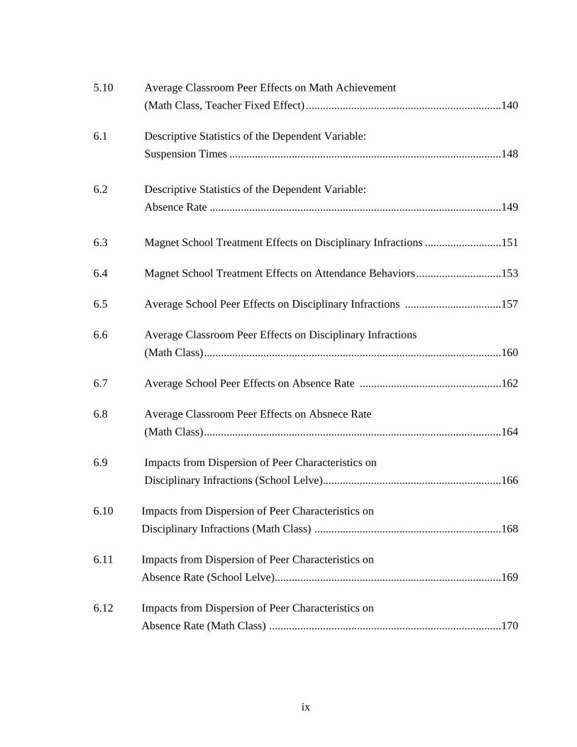
6.13 Heterogeneous Peer Effects on Disciplinary Infractions

(School Level).......................................................................................................172

6.14 Heterogeneous Peer Effects on Disciplinary Infractions

(Math Class)..........................................................................................................175

6.15 Heterogeneous Peer Effects on Absence Rate

(School Level).......................................................................................................177

6.16 Heterogeneous Peer Effects on Absence Rate

(Math Class)..........................................................................................................178

1

CHAPTER I

INTRODUCTION

This dissertation investigates the peer group effects on middle school students’

academic achievement and behavioral outcomes in a mid-size urban district in the South.

The primary objective of this project is to implement credible methodologies to

circumvent the endogeneity problems in peer effect estimation and therefore obtain

unbiased estimates of peer group effects on individual student outcomes.

Peer qualities and peer behaviors have long been recognized as among the most

important determinants of student outcomes. As early as 1966, Coleman and his

colleagues have demonstrated the importance of student composition on individual’s

achievement. In the well-known report Equality of Educational Opportunity, Coleman et

al. (1966) write:

“(Finally), it appears that a pupil’s achievement is strongly related to the educational backgrounds and aspirations of the other students in the school. ………” (p.22) “Attributes of other students account for far more variation in the achievement of minority group children than do any attributes of school facilities and slightly more than do attributes of staff”(p.302)

Aware of the importance of peer impacts, both families and policy makers have included

peer quality as a prominent element in educational decision making. For example,

parents tend to seek for better companions for their children through residential choices

and other school choice options. Many controversial education policies, such as vouchers,

school desegregation, and ability tracking, intend to improve student performance

through changing the composition of peers.

2

However, identifying peer effects is a very difficult task. The most problematic issue

is that families and students usually choose schools and peer groups where they share

similar attributes with other members. Therefore, measures of peer characteristics may

just signal other unobservable individual factors that also affect the outcomes, such as

student willingness to work and parental ambition and resources. This endogenous choice

leads to a selection bias problem. Another problem is that an individual’s outcome and

that of his peers are formed simultaneously --- a student’s achievement is impacted by the

achievement of his classmates and vice versa. This creates a standard simultaneity bias

problem, also termed as reflection problem by Manski (1993). In addition, inference

about peer effects is particularly vulnerable to a general misspecification problem ---

omitted variable bias, due to the fact that both individuals and peers are subject to a

common environment.

Studies attempting to measure peer group effects are susceptible to the endogeneity

biases arising from self-selectivity, simultaneity, and omitted variables correlated with

peer characteristics. Interestingly, in spite of the fact that theoretical articles on social

interaction or peer effects have concentrated most attention on the reflection problems (or

simultaneity bias, e.g. Manski, 1993; Moffit, 2002), selection bias is the most pervasive

methodological issue discussed in empirical studies. The majority of empirical research

on peer effects circumvents simultaneity bias by examining only peer demographic

characteristics (such as race or gender composition) or using lagged values for peer

behaviors or outcomes. Meanwhile, most peer effect studies have focused on reducing or

eliminating selection bias by implementing a variety of creative techniques, such as

3

instrumental variables (IV), fixed effect models (FE), and randomization experiments

(RA).

In the most recent two decades, efforts to identify peer effects on student outcomes

span social science. However, thus far, they have not reached a consensus. For example,

Evans, Shwab, and Oats (1992), using instrumental variable methods, find no significant

school peer effects on teenager behaviors. Hanushek et al. (2003) estimate moderate peer

effects on student achievement in Texas schools. They tackle across-school selections by

implementing fixed effect strategies, and eliminate simultaneity problems by using

lagged measures of peer achievement. Two studies by Sacerdote (2001) and Zimmerman

(2003) use randomly assigned college roommate data and find a significant association

between roommate academic attainment and individual achievement.

Among all the methods to reduce selection bias, randomization is the most credible

one. In a randomized experiment with participants arbitrarily assigned to a treatment

group (for example, a choice school) or a control group (a neighborhood school),

differences between the individuals in the two groups arise solely by chance, which

ensures the endogeneity of peer group formation. Peer group effects therefore can be

ascertained from examining how the peer composition differences between the treatment

group and the control group influence individual outcomes.

In recent years, the administration of school choice programs often provides good

opportunities of studying peer effects with randomization approach. In many school

choice programs, the admissions are conducted through lottery when the choice schools

are oversubscribed --- the unsuccessful lottery participants who enroll in the

neighborhood school can then serve as the natural control group for the purpose of

4

measuring the peer group effects on student outcomes. This approach is used in the study

by Cullen and Jacob (2007), who find no evidences that lottery winners to higher quality

schools (measured by average peer achievement) are better off in academic achievement

than those who lost the opportunity to go to the selective schools.

In this study, I will exploit randomization via magnet school admission lotteries to

examine the peer group effects on student outcomes at both school and classroom levels.

The district studied operates magnet programs at three levels---elementary, middle, and

high school. This study will focus the peer effect investigation on middle school students

(from grade 5 to grade 8) because the state end-of-year assessments have been most

consistent from grade 3 to 8. The district conducts separate lotteries for each magnet

school to determine admission. Students who apply for the district-operated magnet

schools are randomly assigned to either a choice school or a neighborhood school;

conditional on the attendance zone, students are also randomly assigned to the peers in

either the choice school or the neighborhood school. Randomized lotteries therefore bring

an exogenous source of variation in peer characteristics and will be exploited to

overcome the critical issue of selection bias in identifying peer effects.

Under an ideal situation when there is only one magnet school and one neighborhood

school and all participants fully comply with the lottery assignment, peer effects can be

estimated directly from the average differences between the treatment group (magnet

school) and the control group (neighborhood school). However, similar to many other

social experiments, the lottery-induced admission process in the district studied also has a

lot of complications. First, the lottery school enrollment process is voluntary and

participants do not fully comply with the lottery assignment. For example, lottery winners

5

may not enroll in the choice school; lottery losers seek for other options like private

school. With the existence of non-compliance, the lottery-induced admission can no

longer be considered as a pure randomized experiment. Second, the district operates more

than one magnet programs at middle school level. Although a student can only enroll in

one magnet school, a lot of students applied for multiple lotteries. Third, in the years of

investigation, there are significant student attritions among the lottery participants.

Particularly, the attrition rate is higher among lottery losers than lottery winners. Forth,

peer effects may be confounded with student’s heterogeneous responses to magnet school

treatment effects, or may be proxies for some unobserved school factors, such as the

quality of teachers. For example, if less effective teachers tend to be assigned to schools

(classrooms) with high proportion of low SES students, peer effects are likely to signal

teacher quality.

Due to all the complications, even the lottery-induced randomization can not ensure

the exogeneity of the peer compositions. Therefore, instead of simply comparing the

outcomes of winners and losers with different peers, this study exploits the randomized

admission lotteries to form an instrument variable for the regressor of interest --- the

actual peers, and estimates the causal relationship between individual outcomes and the

peer groups from the instrumented (exogenous) peer variables. The model controls for a

large number of individual and school characteristics to improve the precision of the

regression models and eliminate the biases from attrition. In order to test if peer effects

are just signals for teacher impacts, I will also include teacher fixed effects in the

analyses. In addition, the models will control for the interaction between treatment

indicators with observable individual characteristics to examine if peer effects are

6

confounded with heterogeneous responses to treatment effects. Like many other

empirical studies in peer effects, this study will circumvent the simultaneity problem by

using pre-determined peer characteristics (such as race, gender, and social economic

status in peer composition) and lagged measures of peer outcomes.

This dissertation examines the impacts of peer groups on both student academic

achievement (measured by math and reading test scores) and student behavioral

outcomes (measured by student absence rate and disciplinary infractions). The

investigation of peer effects is conducted at both school and classroom levels.

Specifically, the dissertation will answer the following research questions:

1. What is the impact from average peer characteristics on individual student

outcomes at both school and classroom levels?

2. What is the impact from the dispersion of peer characteristics on student

outcomes at both levels?

3. To whom do peer effects matter the most --- which subgroup of student

population are more significantly impact by the peer characteristics?

The rest of the dissertation will be organized in the following manners: Chapter II

provides a review of relevant literature. The theoretical research review presents the

canonical model for peer effect estimation and explains the three major methodological

challenges in identifying peer effects; and the empirical research review examines the

existing evidences from some selective studies in peer effects, with a focus on the

strengths and weaknesses of the methodologies used in these studies. Chapter III

describes the district under study and its magnet programs, presents the data sources, and

most importantly, explains the analytical strategies. The discussion of the methodology

7

includes peer effect identification strategies at both school and classroom levels. It will

start with the basic models under the strict assumption of a pure randomization, followed

by the 2-stage least square (2SLS) IV models with the relaxation of that assumption.

Chapter IV presents the results of school level peer group effects on student academic

achievement. The findings will include the average peer effects, the impacts from

dispersion of peer characteristics, and the heterogeneous peer effects on students in

different subgroups. Chapter V reports the findings of classroom peer effects on student

academic achievement, and compares the results with those from school level analyses.

Chapter VI provides the findings of peer influences on student behavioral outcomes at

both school and classroom levels. Finally, chapter VII summarizes the findings, discusses

the methodological contributions and political implications of this study.

8

CHAPTER II

REVIEW OF THE LITERATURE

This study exploits randomization through admission lotteries to examine the

relationship between peer composition and student outcomes. As such, the review of

literature focuses on previous estimates of peer group effects. The first part of this

chapter reviews theoretical studies on social interaction and peer effects in schools. It

begins by defining peer group effects, describing the multiple channels through which

peers affect student outcomes and presenting the methodological challenges in

identifying peer effects. The second part of this chapter provides an overview of the

existing evidences on the nature and quantitative importance of the association between

peer group composition and student outcomes in academic and behavior. The review of

empirical studies will focus on the methodological strengths and weaknesses.

Conceptual Framework

Peer effects, neighborhood effects, and other non-market social influences are

generally termed as ‘social interactions’--- the impact on one individual of the attributes

or actions of other group members (Moffit, 2001). Peer effects in education usually

include the impact of social interactions between individual student and other students in

the same school or classroom, rather than the interactions between the student and

families or teachers.

9

The mechanisms through which peer groups affect individual’s academic

achievement are complex. Peers not only influence individuals directly through student

teaching, role modeling, or classroom disruption; they also impact individual students

indirectly through the perceptions of teachers and administrators on the peer groups. For

example, if a teacher thinks one particular socioeconomic group is academically weak,

she may lower her expectation and slow down her curriculum in a classroom with a high

proportion of students from that group, which therefore may negatively affect an

individual student’s performance, regardless of that student’s own SES status.

In an influential article on the topic of social interaction effects, Manski (1993)

proposes that the relationship between one individual’s behavior and other group

member’s behavior comes from three distinct effects. Here, let’s apply the concepts to

peer effects in education:

a. Endogenous effects (or simultaneous effects)—a person’s behavior varies

with the mean behavior of the peer group. For example, the propensity of a

student graduating from high school will be impacted by the proportion of

students graduating from high school in the same school.

b. Exogenous effects (or contextual effects)—a person’s action varies with

the exogenous characteristics (pre-determined characteristics) of the peer group.

For example, the propensity of a student graduating from high school will be

affected by the average level of mother’s education of other students in the

school.

c. Correlated effects—persons in same group tend to behave similarly

because they are subject to a common institutional environment or they share the

10

similar characteristics. Literature often terms the shared institutional settings as

‘common shocks’---for example, that all students in the same classroom do well

academically may reflect nothing but the high quality of the teacher. The other

part of the correlated effects, ‘the shared characteristics’, draws a lot of interest

from empirical studies. It is called ‘selection problems’, which arises when

individuals tend to self select into a group with members sharing similar

attributes. For example, families that are very supportive of children’s education

are more likely to sort themselves across schools in order to seek for better peers.

Accordingly, research studying peer effects typically models the behavior (or

outcomes) of an individual (e.g., educational outcomes, criminal behavior, or teen

childbearing), as a function of the average behavior of his/her social group, the

individual’s own characteristics, and also the characteristics of the group:

ijjijijijij ZXXyy (2.1)

where ijy represents individual behavior, like test scores, for individual i in school j; ijy

is the average test scores for peers of student i in school j; ijX are a vector of mean pre-

existing peer characteristics of student i in school j; ijX are a vector of individual or

family characteristics of student i in school j, including gender, race, and social economic

status; jZ are school level characteristics, such as teacher quality and school policies etc.;

ij is an individual error term. In the language of Manski (1993), the coefficients

reflects the endogenous effects, the coefficient reflects the exogenous or contextual

effects, and the coefficient of then reflects the correlated effects.

11

However, Manski (1993, 1999, and 2000) demonstrates that without severe

restrictions, the standard single equation approach like model (2.1) is unable to separately

identify the causal peer group effects from other influences. The key issue, according to

Moffit (2001), is that peer effects are endogenous. The endogeneity, as Moffit further

explains, arises from three problems:

Simultaneity problem: simultaneity bias is also called reflection problem

by Manski (1993, 1999, 2000), which arises from the endogenous effects wherein

one person’s actions affect other group members’ actions and vice versa. As a

simple illustration, in the linear-in-mean model discussed in above, while we

assume that the average achievement of peers affects individual achievement

through the coefficient , individual i also influences the average achievement of

the peers if a symmetric equation holds for every students in the group. As a

result, the individual error term ( ij ) is mechanically correlated with the peer

effect variable ijy , which leads to an inconsistent estimation of peer parameters.

Due to this simultaneous nature, it is extraordinary difficult to identify the causal

effects of peer interactions using contemporaneous peer behavior or outcome

measures without severe restrictions.

Omitted unobserved factors or measurement error: Omitted variables

problem or measurement error occurs when a determinant of the student’s

outcome is omitted or measured poorly in the model. Omitted variables bias is a

common misspecification to all types of regression models---it is virtually never

possible to include all relevant factors in a model. However, due to the correlation

effects, omitted variable bias is particularly damaging to the inferences of peer

12

effects (Hanushek et al., 2003). For example, students in a same school are

subject to similar environment and experiences. Therefore both individual’s and

peers’ achievement will tend to be affected by the common omitted factors, which

may induce a correlation between the peer variables and the random error terms

for all students. It will lead the false attribution of common behavior among

students in the same school to peer influences, whereas, in truth, the students have

similar behavior just because they are subject to a common (unobserved)

environment, such as high-quality teachers.

Endogenous membership problems: it is usually called selection bias or

group endogeneity in the literature; and it is the most pervasive methodological

issue discussed in empirical studies. The peer group itself is often the matter of

individual choice---families and children usually choose being in a neighborhood

or school where they share similar attributes with other members. Within a

school, student placement across classes is also influenced by school policies as

well as parental involvement. Under this circumstance, measures of peer

characteristics may proxy for other unobservable factors that also affect the

outcomes, such as student willingness to work, or parental ambition and

resources. However, those family factors are usually unobservable to researchers.

A standard approach that ignores the endogenous parental choices might

erroneously attribute the entire increment in students’ performance to the superior

peer group.

Given the multiple mechanisms through which peer group impacts student outcomes,

one would predict a strong relationship between peer qualities and student achievement.

13

However, these sources of endogeneity biases make it difficult to identify peer effects. As

Rivkin (2001) argues, regardless of the number of included covariates, single equation

methods almost certainly do not identify true peer group effects. Therefore, in order to

overcome the endogeneity problems, empirical studies on peer effects have attempted to

search for alternative techniques.

Previous Research

Coleman Report (Coleman et al. 1966) is one of the earliest studies on peer group

effects in education. In particular, Coleman and colleagues indicate that black students

performed better academically if they were in schools with higher fraction of white

students. Winkler’s study (1975) finds that both white and black student’s scholastic

achievement is positively related to peer social economic composition; and especially,

transferring from a predominantly black school to a school with lower black population

adversely affects the achievement of black students. Two studies in the 70s by Summers

and Wolf (1977), and Henderson, Mieszkowski and Sauvageau (1978), have shown that

students achieve higher if they are placed with high performing peers. However, the early

studies take few steps toward addressing the endogeneity problems.

In the past two decades, a growing literature has adopted a variety of innovative

techniques to circumvent the methodological challenges in estimating peer effects.

Despite the differences among all the methods used in recent studies, the key to

overcoming the endogeneity problem is to find exogenous sources of variation in peer

composition. The following review will focus on the strengths and weaknesses of

identification strategies in some selected studies.

14

Because this study examines peer group effects on both student academic

achievement and behavioral outcomes, the literature review also includes previous peer

effect studies on both outcomes.

Peer effect on student academic achievement

Relying on longitudinal panel data from Texas, Hoxby (2001) estimates substantial

peer effects on student achievement by comparing the idiosyncratic variations in adjacent

cohorts’ race and gender composition within a grade within a school. The author argues

that the identification strategies are credibly free of selection biases because the between-

cohort peer variations are beyond the easy management of parents and schools. However,

Hanushek et al (2009) examined the same data set and pointed out that the between-

cohort peer composition changes actually come from frequent student transfers rather

than birth or biological rate differences. Student transfers, however, are related to some

unobserved family factors that also impact student achievement. If it is the transfers that

cause the variations in peer characteristics, Hoxby’s method can not eliminate the

endogeneity of family selection. Another study by Lavy and Schlosser (2007) uses very

similar strategies to Hoxby’s to examine classroom level peer impacts, and find that a

high proportion of female classmates improve both boys’ and girls’ academic

performance. Both studies avoid simultaneity bias by only examining predetermined peer

characteristics, such as peer race and gender.

Hanushek and colleagues (2003) also investigate school level peer effects using the

same set of Texas data as Hoxby; but they implement different techniques to address the

endogeneity problem. Their study eliminates the across-school sorting problems by using

15

fixed effect (FE) methods, and circumvents the reflection problems using lagged peer

achievement measures. As argued by the authors, fixed student effects account for all

systematic and unobservable time-invariant individual and family factors that may

influence the residential choice as well as student achievement, such as individual ability

and parental motivations; fixed school effects are correlated with peer composition

through school and neighborhood choices. The paper finds moderate effects of average

peer achievement on student learning, but no impacts from average peer economic status

or the dispersion of peer achievement. Fixed effects are also used in other school level

peer effect studies by Hanushek et al. (2009), McEwan (2003) and Ammermueller and

Pischke (2006).

Fixed effects are widely used in studies investigating classroom peer effects to

overcome the self-sorting problems. For example, Burk and Sass (2004) measure the peer

influences on mathematic achievement within specific math classrooms for middle school

students in Florida. Both student and teacher fixed effects, as well as school/grade and

year fixed effects are included in the regression. Based on the findings that adding

teacher fixed effects purges away the peer influences, the authors argue that the apparent

peer impacts found in other studies may just reflect the endogenous matching between

teachers and students within a school. Other classroom peer studies using fixed effect

method include Betts and Zau (2004), Vigdor and Nechyba (2004), Stiefel, Schwartz, and

Zabel(2004), and Sund(2009). Using fixed effects is expected to remove the spurious

correlations between the time–invariant unobservables and the peer measures. However,

despite its popularity, fixed effect models are not able to overcome the endogeneity that

results from time varying factors, such as the year-to-year shocks.

16

Some studies examine how student performance is impacted by externally induced

changes in peer composition. For example, Angrist and Lang (2002) find that classroom

composition changes brought by Boston METCO program only moderately impacted

minority students’ achievement in reading and language. The METCO program

transferred and randomly placed inner city students to some suburban schools and

therefore introduced plausible exogenous sources of variation in peer composition.

Similarly, Imberman and Kuglar (2008) estimate how the influx of hurricane Katrina

evacuee students impact the performance and behavior of non-evacuee (native) students.

Another conventional approach to deal with selection bias problem is by the

implementation of instrumental variables (IV). For example, in order to address the non-

random classroom assignment problem, Lefgren (2004) instruments the covariates of

peers with the interaction between student’s initial ability with school tracking policy.

The author also uses lagged peer achievement measures to overcome simultaneity bias.

This study suggests modest peer effects--- moving from a 10th percentile classroom to a

90th percentile classroom would only increase the achievement gains by between 0.03 and

0.05 grade equivalents.

Several other empirical studies on school peer effects have also used IV method to

address the endogeneity problems caused by simultaneity and self selection. For example,

Case and Katz (1992), and Gaviria and Raphael (1999) instrument the average peer

behaviors using the average background characteristics of the peers to solve the

simultaneity problems; Boozer and Cacciola (2001) use the fraction of students

previously randomly exposed to small class treatment as the IV for the contemporaneous

peer group measures; Kang (2007) examines the classroom peer effects in South Korea

17

by implementing an IV model that uses the mean and standard deviation of peer science

scores as the instruments for the variable of interest---average classmate math test scores.

The study by Evans et al. (1992) is one of the early studies using IV method to address

group endogeneity (self-selection) problems, wherein a set of metropolitan area social

economic indexes are used as instruments for the peer variable ‘proportion of

economically disadvantaged students at a school’. The study finds significant peer effects

from the simple OLS model, but no impacts from the IV model. However, Rivkin (2001)

questions the validity of instruments used in Evans et al. He examines the same research

question using similar set of instruments but different data set. His findings suggest that

using aggregated metropolitan area characteristics as instruments actually increases the

magnitude of group selection biases. Another peer effect study by Fertig’s (2003) tackles

the potential endogeneity arising from both selectivity and simultaneity by utilizing two

sets of instrumental variables: the first set of IVs indicating school policy in selecting

students upon entry and whether it is a private school; the second set of IVs including

measures of parental caring behavior. Fertig’s study finds that individual student reading

achievement is negatively impacted by the achievement heterogeneity in school peer

composition.

A new stream of empirical literature focuses on special cases where individuals are

randomly assigned across groups. Among all the methods intending to reduce selection

bias, randomization is the most credible one--- it ensures that peer group formation is

totally exogenous. Two frequently cited studies are conducted by Sacerdote (2001) and

Zimmerman (2003), who find significant association between roommate academic

attainment and individual achievement using randomly assigned roommate data at

18

Dartmouth University and Williams College respectively. However, due to the limited

experimental data in social sciences, randomization methods are only applicable to a few

special cases, such as college freshman roommates, or government assisted housing

programs (e.g., in Katz, Kling, and Liebman, 2001), where a central authority conducts

the group assignment.

The random assignment (RA) approach is rarely seen in research on pre-collegial peer

effects. One exception is the study by Boozer and Cacciola (2001) relying on the random

assigned classroom data in Tennessee STAR program to investigate the impact of

average classmate achievement on student own performance. Unlike most other empirical

studies, this study examines the endogenous peer effects --- effects from average

contemporaneous classmate achievement. Since randomization eliminates selection bias,

the authors use instrument variable methods to tackle the simultaneity problems: the

fraction of classmates previously exposed to small-class treatment is formed as

instrument. A possible flaw of this study is that the authors did not address issues that

may affect the purity of the randomization, such as selective attrition and student mobility

between class types. Two other studies using random assignment approach to examine

peer effects on student outcomes focus on classrooms in other countries. (e.g., the South

Korea study by Kang, 2007; and the Kenya by Duflo, Dupas, and Kremer, 2008)

Vigdor and Nechyba (2008) recently present a new method attempting to disentangle

the true peer effects and the effects from selection. Based on the observed peer

characteristics, they predict the probability of random assignment of students across

classrooms, which then enter the model as a predictor of selection effects by interacting

with the peer variables. Similar to many other studies, reflection problems are eliminated

19

by using previous peer achievement measures. Their results suggest that a great portion

of peer effects from OLS estimation actually reflect selection.

Peer effect on behavioral outcomes

Researchers in education have been interested in how peer composition impacts both

individual’s scholastic and non-scholastic outcomes. Due to the limitation in data access

to individual behavioral outcomes, many empirical studies have to rely on survey data to

examine peer influences on student conducts. For example, Evans, Oats and Schwab

(1992) use National Longitudinal Survey of Youth (NLSY) data and find no significant

correlation between percentage of economically disadvantaged school population and

student behaviors such as teenager pregnancy and high school drop out. Argys (2008)

uses the same data set and finds that female students are more likely to use substances if

they are accompanied by older peers. Two other studies by Gaviria and Raphael (2001,

using National Educational Longitudinal Study (NELS) data) and by Bifulco and

Fletcher (2008, using National Longitudinal Study of Adolescent Health (NLSAH) data )

also investigate peer effects on issues like high school drop out, church attendance,

college attendance, and substance uses. Behavioral outcomes (such as alcohol use,

participation in fraternities, and major choices etc) are also widely examined in peer

effect studies at college level (e.g., Lyle, 2007; Kremer & Levy, 2001; and Sacerdote ,

2000), wherein the outcome variables are usually derived from individual responses to

research surveys.

Existing literature provides little knowledge on peer impacts on student conducts at

elementary and middle school levels. The major explanation for lack of research on this

20

issue is data limitation. Many popular approaches used in identifying peer effects,

including fixed effect models (used in studies by Hanushek et.al., 2003, 2009; Betts and

Zau, 2004) and idiosyncratic between-cohort peer variations (used by Hoxby, 2000; and

Lavy and Schlosser, 2007), require the use of longitudinal panel data; so studies using

these methods have had to rely on state or local administrative data sets, which usually

just provide a small set of student outcomes, mostly limited to test scores. Therefore,

most studies on school peer effects have only focused on academic outcomes. One

exception is the study by David Figlio (2005), which investigates how disruptive

classmates impact student achievement and behavior. The behavioral outcome in Figlio’s

study is represented by whether a student is suspended at least once for more than 5 days.

However, the validity of the instrumental variable (proportion of male students with

female names) used in this paper is questionable.

Like most empirical studies, this paper also concentrates on identifying contextual

effects measured by pre-determined peer characteristics and lagged peer outcomes, which

avoids the simultaneity biases arising from endogenous peer effects. The identifying

strategies then focus on tackling the selection bias problems. Specifically, this study will

combine two approaches used in previous studies --- instrumental variables (IV) and

Randomization (RA). As mentioned before, two sets of dependent variables will be

examined: student academic achievement in both math and reading, and student

behavioral outcomes in discipline and attendance. Next chapter provides detailed

discussion on these two methods and their implementations in this study.

21

CHAPTER III

INSTITUTIONAL BACKGROUND, DATA AND METHODOLOGY

The identification of peer group effects in this dissertation relies on the randomization

through magnet school admission lotteries. This chapter starts with the introduction of the

background of the district under study and its operation of magnet programs. It then lists

all the data sources. Finally, this chapter introduces the analytical strategies and specifies

the regression models to estimate peer effects at both school and classroom levels.

Institutional Background

This study focuses on peer group effects on middle school students in a mid-size

Southern urban district. In the school year 2003-2004, the district serves approximately

80,000 students from kindergarten to 12th grade in 129 schools, with half of the student

population eligible for the federal free or reduced price lunch program. Similar to other

urban school systems in the nation, the district is racially mixed, serving 41% White

students, 47% Black students, and 9% Hispanic students. About 6% students are

categorized as English Language Learners (ELL). Middle schools in this district are

structured from grade 5 to 8, which is one grade earlier than many other districts in the

nation. During 2003-2004 school year, there are approximately 24,500 students in 52

middle schools. The demographic characteristics of middle school students are almost

identical to the whole district population.

22

The district operates magnet schools at all three levels—elementary, middle, and high

schools. There are two types of magnet programs: selective academic magnet (applicants

must meet the grade/test score requirement), and non-academic magnet. At the middle

school level, there is one academic magnet serving grades 5 to 8. While there is another

academic magnet serving grades 7 to 12, it is not considered a middle school magnet in

this study because the lottery to this school happens 2 years later than the other magnet

programs starting from 5th grade. The complications caused by the second academic

magnet school will be addressed later in this chapter.

Students are admitted to a magnet school through four channels: (1) lottery; (2)

sibling preference; (3) geographic priority zones; (4) promotion from a feeder magnet. In

practice, all students eligible for the latter 3 categories are admitted to the magnet school

without going through the lottery. Since the identification strategy relies on lottery

outcomes, the investigation of peer effects in this study will limit to the sample of

students who participated in the admission lotteries to the magnet middle schools.

Students who did not participate in magnet school lotteries are included in the

calculations of peer variables, but are dropped from the regression analysis.

Middle school lotteries are held in the spring of the fourth grade for the following

academic year. The district conducts separate lotteries for each magnet school. Students

can enter multiple lotteries. Students who are accepted outright on lottery day must

decide whether to accept any of the positions offered them --- if they accept a position in

one school, they go to the bottom of the wait list for any other magnets. Those who lost

the lottery on the lottery day are placed on wait lists and will be accepted off the list as

positions become open.

23

The district offers lottery data starting from the spring of 1997, but the achievement

data are available from school year 1998-99 through 2006-07. Because student prior

achievement (measured by 4th grade test scores) is an essential covariate in the analyses,

this study includes the 5 cohorts of students entering 5th grade between fall of 1999 and

fall of 2003.

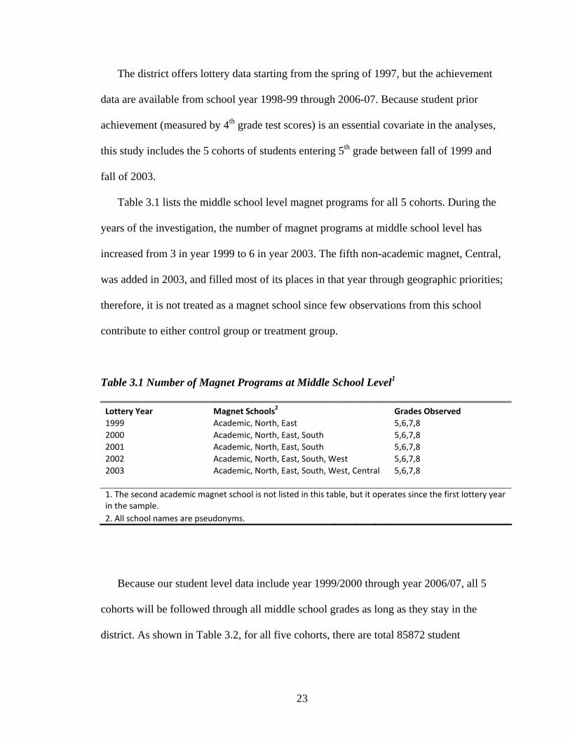
Table 3.1 lists the middle school level magnet programs for all 5 cohorts. During the

years of the investigation, the number of magnet programs at middle school level has

increased from 3 in year 1999 to 6 in year 2003. The fifth non-academic magnet, Central,

was added in 2003, and filled most of its places in that year through geographic priorities;

therefore, it is not treated as a magnet school since few observations from this school

contribute to either control group or treatment group.

Table 3.1 Number of Magnet Programs at Middle School Level1

Lottery Year Magnet Schools2 Grades Observed

1999 Academic, North, East 5,6,7,8

2000 Academic, North, East, South 5,6,7,8

2001 Academic, North, East, South 5,6,7,8

2002 Academic, North, East, South, West 5,6,7,8

2003 Academic, North, East, South, West, Central 5,6,7,8

1. The second academic magnet school is not listed in this table, but it operates since the first lottery year in the sample.

2. All school names are pseudonyms.

Because our student level data include year 1999/2000 through year 2006/07, all 5

cohorts will be followed through all middle school grades as long as they stay in the

district. As shown in Table 3.2, for all five cohorts, there are total 85872 student

24

observations in all middle schools in the district.1 The observations of lottery participants

count for 14-15% of all middle school observations for each cohort; the total number of

participant observations is 12314, which makes up the analysis sample in this study.

Table 3.2 Number of Student Observations in Middle Schools by Cohorts

Cohot1 Cohort2 Cohort3 Cohot4 Cohort5

Enrollment

All Schools 14844 17504 17991 17406 18127

Magnet School

Academic 516 524 571 621 596

North 425 514 408 312 282

South 555 586 589 532

East 302 225 290 326 371

West 250 353

Total 1243 1818 1855 2098 2134

Lottery Participation

Total Participants 2087 2449 2820 2499 2459

Academic 1261 1272 1657 1318 1608

North 860 970 997 927 528

South 1226 1292 1155 903

East 793 707 1021 922 705

West 520 461

Composite Non‐Academic 1246 1821 2020 1831 1530

Note: Counts only middle school students (5th to 8th graders) who were also enrolled

in the district as 4th graders and had non‐missing math test scores in 4th grade.

From lottery year 1999 to lottery year 2003, there were approximately 5000

applications to all middle school magnet programs, among which nearly half applied for

the academic magnet. Table 3.3 describes the lottery outcomes and 5th grade enrollment

patterns for each magnet school. There are two types of lottery winners defined: those

1 Because prior achievement is desirable to be included in the calculation of peer characteristics and in the regression, the counts of student observations are limited to students who were also enrolled in the same district as 4th graders and had non-missing math scores. The actual numbers of student observations are larger for all cohorts.

25

admitted outright on the lottery day and those whose place on the wait list was reached by

the start of the school year23.

As shown in Table 3.3, for the 2306 lottery participants for the academic magnet, the

probability of admission is less than 50 percent. Of the 1201 students not admitted by the

academic school at the beginning of 5th grade, 727 (60%) either did not apply or failed to

win any other magnet programs. Although 40% of the students who lost the academic

magnet lottery were admitted to other non-academic magnet programs, many of them did

not comply with the lottery assignment: only 285 of them chose to attend a non-academic

magnet in 5th grade, compared with 826 enrolled in regular schools. About 19% (437) of

lottery participants did not have test records in grade 5, of whom the majority no longer

attended a school in the district.4

2 Delayed winner is defined based on student original position in the wait list. If a student lost the lottery outright on the lottery day, but his number in the wait list is reached by the start of the school year, the student is defined as a delayed winner. The definition of delayed winner is based on the original wait list because the number on the list is solely determined by the lottery and not by subsequent decisions of students and parents. 3 Accordingly, there are two lottery outcome indicators are defined: outright_winMj=1 if a student is an outright winner of magnet school j, 0 otherwise; delayed_winMj=1 if a student is a delayed winner of magnet school j, 0 otherwise. 4 337 academic magnet lottery participants never enrolled in the district as 5th graders. Another 100 students enrolled in district schools but were not present for testing --- the majority of these students had probably left the system prior to the test date, as 65% of them were never enrolled in 6th grade.

26

Table 3.3 Magnet School Lotteries and Enrollment

Non‐Academic

Academic North South East West Composite Non‐Academic

Lottery Participants1 2306 1307 1384 1260 289 2564

Winners

Outright 884 709 492 511 50 1430 4

Delayed2 221 308 374 326 46 890

Losers

This Lottery 1201 290 518 423 193 397

All Lotteries 727 54 111 73 18 225

Grade 5 Enrollment3

This Magnet 758 391 384 243 30 1048

Other Magnets 285 325 413 430 143 337

Non‐Magnets 826 410 408 406 90 824

Left System/Untested

5th Grade 437 178 172 180 26 347

6th Grade5 149 122 99 93 19 196

1. Lottery participants count only the students who were enrolled in the district as 4th graders

and had non‐missing 4th grade test scores when lottery was conducted.

2. Delayed winners in this table count only the non‐outright winners who received notice before

the 12th day of school year in 5th grade.

3. Counts only students tested in mathematics as 5th graders as well as 4th graders.

4. Win at least one non‐academic magnet lottery

5. Students who were in the district as 5th graders but left the system (or untested) in 6th grade

There were more than 2500 entrants in one or more non-academic magnet lotteries.

Numbers for the West magnet school are very low because this school did not become a

magnet school until the school year 2002/03 and most of its places were actually taken by

students promoted from a feeder school. As we can tell from the table, many students

applied for more than one magnet programs, so the majority of the participants won the

admission opportunity in at least one non-academic magnet, either outright or through

delayed notices. 397 (16%) students did not win a place among all non-academic

programs; but because many of the students also applied for the academic magnet, there

27

are only 225 students who were not admitted by any magnet program, representing 8% of

all non-magnet lottery participants. Regardless of the high admission rate, less than 50%

of participants attended a treatment group school as 5th graders, while 846 were enrolled

in non-magnet schools. About 13% students left the system or were not tested in 5th

grade.

As Table 3.3 shows, there are many complications in this district’s lottery based

admission process: non-compliance, multiple choices, and attrition. All these

complications will threaten the purity of randomization; and therefore, Ordinary Least

Square (OLS) method is not able to obtain unbiased estimates of peer effects. Later

discussion in this chapter will present the solutions to address the problems caused by

these complications.

Data Source

Data for this study are collected from the district’s administrative data system. All the

datasets are student level data, including a rich set of information on individual students,

such as academic achievement, demographic background, course enrollment, lottery

participation, disciplinary infractions, and absence records etc.

(1) Achievement Data. Student academic achievement information comes from the

state annual testing program that includes virtually all students beginning in 3rd grade and

continuing through 8th grade. The tests cover five subjects: reading, mathematics,

language arts, social studies, and science. The assessments adopt the Terra Nova series of

achievement tests constructed and calibrated annually by CTB/McGraw-Hill, with

additional items reflecting special content of the state K-12 curriculum. Achievement

28

data from 4th grade will serve as the prior achievement benchmark for individual students

and will be aggregated at classroom and school levels to calculate academic ability

measures for peers. Student test scores in grades 5 to 8 are used to form the dependent

variables reflecting student academic outcomes.5 Similar to many other empirical studies,

this project focuses on achievement in math and reading.

(2) Course Data. Every year, the district provides a detailed course file, including

information of course code, course id, course title, course period, and instructor name,

etc. The course file reveals the specific class placement for each student in every subject,

thereby identifying the classroom peers. In addition, the course file also enables me to

match a student with his instructor for a specific class, which will be used to estimate

teacher fixed effects to test if peer effects actually represent the impacts of teachers.

(3) Lottery Data. The district provides lottery records of all admission lotteries

conducted for the magnet schools that have oversubscribed applications. The data include

information such as lottery application, lottery results, and wait list number etc, which are

going to be used to create variables indicating lottery participation and lottery outcomes.

Although the data are available from lottery year 19976 through 2003, only lottery

participants from lottery year 1999 to 2003 are included in the sample.

(4) Student Background Data. Another student level data file contains student

background characteristics, such as student gender, race, whether a student is in special

education program, whether a student is an English Language Learner, whether the

5 The achievement data provide scale scores in all subjects. However, we received two sets of achievement data separately: one for school year 1999 to 2004 (received in 2005), and the other for school year 2005-2007 (received in early 2009). The scores in early year data and late year data are differently scaled --- the average scores in later years are lower by 130-150 points for both math and reading. In order to address the inconsistence in test scores, I transformed student test scores (from 4th grade to 8th grades) to standardized scores with a mean of 0 and a standard deviation of 1 in each grade and each year. 6 In our sample, it means the lotteries conducted in the spring of 1997 for magnet schools starting from 5th grade in the fall of 1997.

29

student is eligible for federal free or reduced price lunch program, and student prior

achievement. All the background variables will be included in the regression as

explanatory variables to improve the model precision and deal with the possible biases

arising from sample attrition; they are also going to be aggregated at classroom and

school levels to construct peer characteristics.

(5) Discipline and Attendance Data. The district administrative data also provide

student attendance and mobility records, as well as disciplinary consequences reflecting

the frequency and severity of student misconduct incidents. Two variables are derived

from the attendance and disciplinary records: annual attendance rate, and annual number

of suspensions. The contemporary values (values in grades 5 to 8) of these two variables

are used to form the dependent variables representing student behavioral outcomes. The

lagged values (4th grade) of these two behavioral variables will be introduced as

explanatory variables and will be used to construct peer variables at both classroom and

school levels.

All of the datasets are linked by a unique student identification number and variables

are created to estimate peer group impacts on individual students in middle schools of

this Southern city district. Middle schools are chosen for two major reasons. First, the

achievement data from the state standard test are only available for students in grades 3-

8. Because most elementary schools in the district are structured from Kindergarten to 4th

grade, the elementary sample is much smaller than the middle school sample. Moreover,

focusing on students from 5th to 8th grade, I can use student’s elementary school (4th

grade) records to establish the achievement benchmark. Second, this project is going to

investigate the peer effects at both school and classroom level. In this district, the

30

majority of middle school students (especially when students reach 7th and 8th grade)

typically rotate through classrooms for different subjects. The classroom level

investigation then will estimate subject-specific peer effects, which is different from most

previous studies that examine general class peer effects using data from elementary

schools.

Analytical Strategy

In this study, the identification strategy combines both the instrumental variable

method and the method of randomization. In particular, the lottery outcomes will be

exploited to construct the counterfactual peer variables and the instrumental variables.

This part will first presents a review of the two econometrical methods --- instrumental

variables (IV) and randomization (RA). It will then discuss the analytical models to

answer the three research questions.

Overview of the methods

1. Instrumental Variables

Instrumental variables (IV) method is a frequently used estimation technique in

empirical economic studies (probably second only to Ordinary Least Squares (OLS)

according to Wooldridge (2001)). It was originally proposed by Reiersol (1941), and

further developed by Durbin (1954) and Sargan (1958).

The motivation of using instrumental variables method comes from the fact that OLS

yields consistent estimates only when the error terms are asymptotically orthogonal to the

regressors. For example, in a simple linear regression model:

31

y 0 x1 u (3.1)

If 1̂ is to be consistent for 1 , the condition 0),( uxCOV must hold7. In other words,

OLS obtains consistent estimates only if all regressors are exogenous. However, in

applied econometrics, endogeneity that causes 0),( uxCOV arises from many sources,

such as omitted variables, self-selection, measurement errors, and simultaneity etc. For

example, in peer effect estimation, one regression equation can often have multiple

sources of endogeneity.

The method of instrumental variables provides a general solution to the problems of

endogenous regressors. Valid instrumental variables must satisfy two basic conditions.

First, the instruments must be mean-independent of the error terms. For example, if we

find an observable variable z to be used as instrumental variable for the endogenous

variable x in equation (3.1), it must be uncorrelated withu : 0),( uzCOV . In other

words, the instrumental variable should not be correlated with any unobserved factors

that influence the outcome. The second condition requires that the regressor x depends

on z . In the simple case like equation (3.1), this means 0),( xzCOV --- the instrumental

variable and the regressor of interest must be correlated. In summary, an instrumental

variable is a variable that does not belong in the model in its own right; it must be

correlated with the regressor of interest x and only contributes to the outcome y

through x . When variable z satisfies the two conditions, the parameter 1 can be

identified from the following:

1 ),(/),( xzCOVyzCOV (3.2a)

7 Another condition is E( u ) = 0, but with the existence of the intercept 0, this assumption is for free.

32

Given a sample of data on yx, and ,z it is simple to obtain the IV estimation of 18:

IV1̂ ))(())((11

xxzzyyzz ii

n

ii

n

ii

(3.2b)

IV methods have been used in a number of educational studies to solve the

endogeneity problems. For example, Evans and Schwab (1995) use student’s affiliation

with Catholic Church as IVs to investigate the effectiveness of attending Catholic

schools; Neal (1997) examines the same question using geographic proximity to a

Catholic school as IVs; Hoxby(2000) uses the natural boundaries created by rivers as IVs

for the concentration of public schools within a school district to estimate the impact of

public school competition on student achievement.

Empirical studies using IV approach all face the challenges to justify the validity of

the chosen instruments. A valid instrument must satisfy the aforementioned two

conditions. In general, it is likely that the instruments can meet the second requirement of

being correlated with the regressor of interest 0),( xzCOV ; it is often hard to prove if

the instruments meet the first condition of not being correlated with the error term

0),( uzCOV . For example, in Evans and Shwab’s influential Catholic school paper,

the authors argue for the credibility of using Catholic church affiliation as instrumental

variables from two perspectives: first, being a Catholic strongly affects Catholic school

attendance; second, Catholic families are very close to the national average on a variety

of social-economic indicators --- therefore, the students from Catholic families do not

differ from other students in any way impacting outcomes than attending Catholic

8 In practice, instrument variable estimator is usually estimated from the two-stage least square (2SLS) models: (1) at the first stage: obtain the fitted values x̂ (the endogenous regressor ) from the regression of x on the instrument variable z and other exogenous regressors in the model; (2) at the second stage, run

the OLS regression of y on x̂ and other exogenous regressors.

33

schools. However, as Tyler(1994), Neal (1997) and Altonji et al. (2005) note, being

Catholic may still be well correlated with some less easily measurable neighborhood or

family characteristics that also influence individual outcomes.9

A valid instrument can be found in the context of program evaluation, such as job

training program, or school choice program, wherein a social experiment is usually

conducted to randomly assign individuals to be a control group or a treatment group.

Randomization determined eligibility meets the two requirements of a convincing

instrument: first, individuals are randomly selected to treatment or control groups, so the

eligibility is exogenous; second, in many experiments, being treated is solely determined

by the randomized assignment, therefore the eligibility is strongly correlated with the

regressor of interest --- the treatment.

2. Randomization

In program evaluation or peer effect studies, the counterfactual question asked is what

would have happened to individual’s outcomes if he/she had been placed in another

situation. For example, what would the student math performance be if he attends a

choice school instead of a neighborhood school, or if he stays with a group of high math

performing students instead of with low math performing students? Clearly, the sample

counterparts for the missing counterfactuals are not observable in ordinary data --- the

same person can not be placed in both states in the same time. Therefore, the best way to

identify the causal relationship would be comparing the outcomes of individuals with

nearly identical characteristics (both observed and unobserved) being assigned to

9 In Neal’s Catholic school study, the author uses the geographic proximity to Catholic schools as the instruments for Catholic school attendance. Altonji, Elder, and Taber(2005) examines the validity of three sets instruments used to address the self-selection problems in attending Catholic schools: religious affiliation, geographic proximity, and the interaction between religion and proximity. However, their findings suggest that none of the three instruments are valid in identifying the Catholic school effects.

34

different situations. Randomization makes this realistic. Individuals are randomly

assigned to a treatment group (for example, a choice school) or to a control group (a

neighborhood school); therefore, the control group can be used to estimate the average

outcomes corresponding to the counterfactual state that would happen to the individuals

in the treatment group had they not received the treatment.

For example, suppose there is a school choice program with one choice school

(treatment group) and one regular public school (control group). Let’s assume that a

lottery is the only way through which a student will be enrolled in the choice school. Let

ip be an indicator variable for lottery participation. For all the lottery participants

( 1ip ), let id denote the treatment: 1id indicates that student i is enrolled in the

choice school; 0id , otherwise. Let ir denote the eligibility of the treatment: 1ir

indicates that student i won the lottery and was offered the opportunity to the choice

school; 0ir indicates that student i lost the lottery.

In theory, selection bias does not arise in a randomization-induced lottery program

because winners and losers are identical on average in both observable and unobservable

characteristics. Therefore, for all the lottery participants )1( ip , the causal effect of

being offered the opportunity of treatment (in this case, being accepted into the choice

school) can be directly estimated from a simple OLS model:

iii ry (3.3)

In equation (3.3), ir is determined by the randomized lottery and is orthogonal to the

residual i . The parameter measures the average difference between the outcome of

lottery winners and lottery losers, also known as Intention to Treat effect (ITT). Although

35

equation (3.3) yields unbiased estimation of ITT effect, many empirical studies still add a

set of additional individual characteristics (denoted by iX , including demographic

characteristics and family background etc; for examples, see Cullen et al., (2006, 2007),

Katz et al (2002)) into the equation to improve the model precision:

iiii Xry (3.4)

Because these individual characteristics also impact the outcome variable y i, the

inclusion of iX means that the influence from these variables does not enter the error

term i . Therefore, including the individual characteristics improves the precision of the

estimates on ITT effect by reducing the residual variation.

The intention-to-treat (ITT) estimate measures the impact of being offered treatment.

It is argued that ITT is of the direct interest of policy makers because it is the only policy

variable under control by public officials. For example, policy makers can offer vouchers

for students to attend private schools, but they can not force families who received the

vouchers to actually use them. However, from the perspective of program evaluation, it is

still desirable to estimate the actual impact of treatment (such as choice schools, training

programs) itself, rather than just being offered the chance to get treatment. The average

effect of treatment on the treated (ETT) can be measured from the equation:

iiii Xdy (3.5)

Wherein 1id means that student i actually enrolled in the choice school, and

parameter estimates ETT. In an ideal situation where student enrollment is solely

determined by lottery and all participants comply with the lottery assignments, id equals

ir in equation (3.4) --- ITT and ETT coincide.

36

However, in many social experiments, participants usually do not fully comply with

the lottery assignments: winners may choose not enrolling in the choice school, and

losers may seek for other choices rather than the neighborhood school. In some school

choice programs that offer multiple opportunities (such as the Milwaukee voucher

program and the magnet programs in this study), students may participate in several

lotteries at the same time. Families that win multiple lotteries have to make one choice

among all the choice schools that accept their child; and lottery loser families may also

choose to relocate to another neighborhood or seek for other choices such as private

schools. Under all these circumstances, the differences between the winners and losers

are no longer purely determined by the lottery. Rather, they may be correlated with other

unobserved factors influencing student outcomes. Therefore, in equation (3.5), id is no

longer exogenous and OLS approach can not yield an unbiased estimate of parameter .

This problem can be solved by using lottery assignments )( ir as instruments for the

actual school where the student finally enrolled in )( id . Lottery assignments meet the two

required conditions of valid instrumental variables: because the assignments are

randomly decided, they are orthogonal to the error term; because lottery is the only way

through which the participants can enroll in the choice school, the assignments are highly

correlated with the enrollment variable id . Therefore, ETT can be estimated from a two

stage-least-square (2SLS) model using IV approach:

First, obtain the fitted values id̂ from the regression:

iiii Xrd i (1st stage model, 3.6a)

Second, obtain the IV estimate of parameter (ETT) from the regression:

37

iiii Xdy ˆ (2

nd stage model, 3.6b)

Randomization has been exploited by a number of studies to examine the impact of

educational policy/reform on student achievement. For example, Cullen and colleagues

(Cullen, Jacob, and Leavitt, 2003; Cullen and Jacob, 2007) estimate the ITT effects of

Chicago public school choice program. Rouse (1998) and Howell and Peterson (2002)

examine the impact of private school voucher plans using lottery assignments as

instrument. Kruger (1999) also exploits randomized assignment as an instrumental

variable to evaluate the class size reduction program in Tennessee STAR experiment.

Identification strategies in this study

As many other social experiments, the lottery-induced randomization in the

understudy district also has lots of complications: first, the lottery school enrollment

process is voluntary and participants do not fully comply with the lottery assignment;

second, in many school choice programs, students can apply for multiple schools; third,

in the years of our investigation, there are significant student attritions in both lottery

winner and loser population; forth, student’s responses to peer impact are hetergenous;

finally, peer effect may signal some unobserved school factors, such as teacher qualities.

Therefore, instead of simply comparing the outcomes of winners and losers with different

peers, this study exploits the randomization through admission lotteries to form an

instrument variable for the regressor of interest --- the actual peers, and estimates the

causal relationship between individual outcomes and the peer groups from the

instrumented (exogenous) peer variables. The model also controls for a large number of

individual and school characteristics to improve the precision of the regression models

38

and eliminate the biases from attrition. In addition, fixed teacher effect will be included to

test if the peer variables signal for teacher quality.

The following sections will discuss the analytical models identifying peer group

effects on student outcomes. The discussion will start with school level average peer

effect estimation, followed by classroom average peer effect analysis, the estimates of

effects from dispersion of peer characteristics, and the heterogeneity in peer group

impacts.

1. School level analysis

I. Basic models and variables

a. Basic models

The basic idea of the identification strategy is to estimate peer effects from the

differences between the actual peers of a magnet school student and his counterfactual

peers in a neighborhood school he would have attended had he not been enrolled in the

magnet school. Since one student can not attend both magnet school and neighborhood

school simultaneously, the counterfactual peers are not observable. However, we can

exploit the randomized admission lottery for the magnet school to construct the

counterfactual peer values. In this district, the admission lotteries randomly assign

participants to magnet schools and neighborhood schools; conditional on the attendance

zone, the lottery also randomly assign participants to peers they will encounter. If all

lottery participants fully comply with the lottery assignments, the peers for the lottery

losers who enrolled in neighborhood schools can serve as the counterfactual peers for the

magnet school students. Peer effects then can be estimated from the average differences

39

in outcomes associated with the treatment group (magnet school) peers and control group

(neighborhood school) peers.

To facilitate the explanation, let’s make some assumptions first: (1) All participants

are randomly assigned to treatment group (magnet school) and control group

(neighborhood school), and fully comply with the lottery assignment; (2) The treatment

group only includes one magnet school; (3) The indicator for lottery outcomes is binary:

win or lose. The outcomes of individual student i in school j can be estimated from the

model:

ijjiij uPXY )( (3.7)

where iX is a vector of observed student characteristics; jP represents the peer

characteristics in school j; iju is the error term for student i in school j10.

Under the assumptions, student i would attend a neighborhood school (N) if he does

not enroll in a magnet school (M). Therefore, the outcomes are ),( iNiM YY , which can be

obtained from:

iMMiiM uPXY )( (3.8a)

or

iNNiiN uPXY )( (3.8b)

Determined by the lottery, a student is assigned to either MP (peers in the magnet school)

or NP (peers in the counterfactual neighborhood school where student i would attend if he

had not been in the magnet school). Let 1id if student i enrolls in magnet school M (in

10 There are two components included in the error term iju : the school effect on all students enrolled in

school j, and the idiosyncratic error for student i.

40

treatment group); 0id if in neighborhood school N (in control group). Then we can

combine equation (3.8a) and (3.8b) together:

iNiNiMiiNiMiij udPdPduuXY )]1([)()( (3.9)

where iiNiM duu )( represents the magnet school treatment effects

and )]1([ iNiM dPdP represents the peer impacts on student outcomes.

Because N varies across students, the treatment indicator id is heterogeneous. Let’s

rearrange the model by defying )1|( iiNiM duuE as the mean expectation of

treatment effects over the students who received treatment and

)1|()( iiNiMiNiMi duuEuu as the heterogeneous responses to treatment:

iNiiiNiMiiij uddPdPdXY )]1([)( (3.10)

Now there are two components in the error term iid and iNu .

Although the lottery randomly assign student i to either MP or NP , NP itself is a

matter of parental choices, especially residential location decision. Thus, it may be

related to other unobservable factors that also affect student outcome, such as family

resources, and bias the estimation of the peer effect . If we can control for the

correlation of NP and the error term iNu , this source of endogenous bias can be

eliminated. So let )|( NiNN PuEP denote the correlation between NP and iNu , including

NP into the equation:

iNiiNiNiMiiij vdPdPdPdXY )]1([)( (3.11)

41

where )|( NiNiNiN PuEuv . With NP controlled in the model, the new error term iNv is

no longer correlated with the peer measures --- the coefficient now does not pick up

the endogenous bias from NP .

Equation (3.11) includes two peer variables: the first term )]1([ iNiM dPdP

representing lottery-based variation in peers, and the second term NP representing

residence-based variation in peers. The coefficient on the former term measures the

causal relationship between peers and student outcomes. Note from equation (3.11) that

the estimation of peer effect depends on the treatment variable id . Under the

assumptions, the value of id is randomly determined by the magnet school admission

lottery; conditional on NP , the lottery also randomly assigns students either to MP or

NP .

Therefore, given that NP is included in the model, both the treatment term id and the peer

term )]1([ iNiM dPdP are exogenous --- OLS estimation of model (3.11) can yield

unbiased estimation of peer effects11.

However, also note that peer variable NP represents the counterfactual non-magnet

school peers with whom a student would stay if not enrolled in a magnet school.

Therefore, NP is not observable for students who attended the magnet school. The next

step then is to predict the counterfactual peers NP for magnet school students. The

prediction is based on the sample of students who lost the lottery and attended regular

public schools, using their information in vector X as well as their elementary schools.

So a student in the magnet school get assigned an predicted value of NP̂ , which is close to

11 Equation (3.11) is considered as the basic model estimating school level peer effects. Other regressors included in the final regression model (not shown in the equation due to text limit) include the lottery participation indicators (including lottery year and lottery school combination), year and grade indicators.

42

the actual NP of a counterpart student (a lottery loser attending a neighborhood school)

who share similar background (such as demographic characteristics and elementary

school) with this magnet school student12.

b. Variables

The dependent variable ijY includes both student academic achievement as well as

behavioral outcomes. Individual academic achievement as dependent variable is

measured by the standardized test scores based on the distribution of original scale scores

in each grade and each school year. The behavioral outcomes are measured by student’s

total numbers of suspension and the absence rate in each school year.

The vector X includes student demographic variables as well as previous test scores

and behavioral measures: black, female, low income (measured by eligibility for the free

and reduced-price lunch program), special education, ELL, 4th grade reading and

mathematics test scores, and 4th grade disciplinary incidences and absence rate.

The regressors of interest cover a rich set of attributes of the peer groups. The

specifications not only include the most commonly expressed peer characteristics such as

race, gender, social economic status (SES)compositions and peer academic abilities, but

also include less commonly examined characteristics such as percent special education

student, percent ELL students, peer disciplinary infractions and attendance behaviors.

The contextual (exogenous) peer characteristics, such as race, gender or SES

compositions, are constructed by averaging over all individual students at each grade in

every school. The endogenous peer characteristics, including both peer achievement and

12 Detailed discussion on the prediction of NP is provided in Appendix A, which includes the regression

model that predicts NP , and the descriptive statistics comparing the predicted value and the actual value of

NP for some lottery losers.

43

behavioral outcomes, are constructed as the aggregate mean of lagged values of the

outcome variables (both academic achievement and behavioral records in 4th grade). As

noted before, the main reason of using lagged peer outcomes is to avoid the mechanical

peer correlation arising from reflection problems. Another reason of relying on peer

outcomes in 4th grade is because these values are determined before the admission

lotteries that assign participants to treatment and control groups. Therefore, it not only

circumvents the simultaneity bias, but also reduces the possible biases from omitted

variables that are correlated with both individual outcomes and the peer variables since

these peer outcomes are predetermined before students enter middle schools. However,

although lagged values of peer outcomes are expected to capture most of the relevant

variation in current peer achievement and behavior, they are still not perfect proxies for

the current values. As Hanushek et al. (2003) suggested, the estimated effects from the

lagged peer behavioral variables are most likely to be downward biased given the fact

that the current innovations to behavior form an important avenue through which peers

affect outcomes; therefore, the estimated effect of lagged peer behaviors may just provide

a lower bound estimate of current peer behaviors.

The regression models require multiple versions of peer variables for each student:

MP and NP for school level peers. MP will be calculated straightforwardly using students

actually enrolled at M, but NP is an estimated variable for magnet school students. In

order to avoid introducing a difference between students whose NP is observed (lottery

losers) and those whose NP is a counterfactual (lottery winners), the predicted NP̂ ’s will

be used in the final models for all students.

44

The main treatment indicators id are dummy variables for enrollment in a magnet

school. Students are regarded as enrolled in a magnet school if they finished the school

year at the magnet. The relatively small number of students who started the year at a

magnet before transferred out are treated as non-magnet students.

All models include a full set of grade by year interactions in order to control for

differences in test forms across grades and year. In addition, a set of lottery participation

indicators are also controlled in all models because there are separate lotteries for each

magnet school, and randomization only happens to the participants in a given lottery.

II. Relax the assumptions

From now on, let’s relax the provisional assumptions. First, there are some non-

compliers among the lottery participants. The self selection of non-compliers means that

the treatment variable id is no longer exogenous and neither is the peer term. Therefore,

OLS methods will not yield unbiased estimates of model (3.11). The solution for this

problem is to implement an instrument variable model, in which the lottery outcomes are

used to construct the instrument variables. The following is the first stage models to

predict the endogenous covariates (both treatment indicator and the peer variable) using

the instrumental variables:

(a) Estimate magnet school treatment variable d i from model

iiii Xrd (1st stage IV model1)

where the lottery result indicator r i serves as the external instrument variable ( ir =1

if student i won the lottery; 0 otherwise).

(b) Estimate the peer variable )1( iNiM dPdP from model:

45

iiiMNiMMiNiM XdPdPdPdP )]ˆ1(ˆˆ[)1( (1st stage IV model2)

Where the external IV for the endogenous peer variable is )]ˆ1(ˆˆ[ iMNiMM dPdP .

The instrument variable includes three parts: iMd̂ is an prediction of the probability

that student i attend the magnet school, which is estimated based on students’

lottery outcome indicators and demographic variables13; MP is the mean value of

school level peer variables in the magnet school; and NP̂ is the estimated school

level peer variable in the neighborhood school.

If we replace the endogenous regressors with their IV estimates, the instrumented model

(second stage model) can now be expressed as:

iNiiNiNiMiiij vdPdPdPdXY ˆˆ)]ˆ1(ˆˆ[ˆ)( (2nd stage model, 3.12)

Given the use of lottery outcomes as instruments and the inclusion of NP̂ in the

regression, we obtain unbiased estimates of peer effects free of self-selection bias even

with the lottery non-compliance.

Let’s now relax the second assumption. Instead of having one magnet program and a

single lottery, the school district operates multiple magnet schools, including one

academic magnet program and several non-academic magnet programs. Separate lotteries

are conducted for each school. Although a student can only attend one magnet school,

lots of students apply for multiple lotteries, which causes three problems: (1) Because of

multiple lottery applications, the chances for a student failing to obtain a place in at least

one of the non-academic magnet schools are small; therefore, the counterfactual sample

13 Appendix B provides the prediction models for iMd̂ , the detailed procedures of calculating iMd̂ , and the

descriptive statistics.

46

is small and thus the power of detecting the treatment effects and peer effects in each of

the non-academic magnet school is limited. (2) When the groups are small, the individual

characteristics among treatment and control groups are likely to be unbalanced even with

random assignment. (3) Lottery outcomes are multivalued for students who apply for

several lotteries, which challenges the validity of lottery outcomes as instruments for id .

The first two problems do not bias the estimations on and , but they increase the

sampling error. Combining several non-academic magnet programs into one single

treatment provides the solution14: it increases the sample sizes of both treatment and

control groups. In addition, including individual variables )( iX in the regression also

corrects the imbalances on these characteristics between treatment and control groups.

The third issue is most problematic. For lottery outcomes to be a valid instrument for

the treatment variable id , it is required that ],1|)1|([ iiMiMiMiM RddEE

]1|)1|([ iMiMiMiM ddEE 0 . That is, the lottery outcome variable iR should not

carry any information about the heterogeneous response term iid . However, there are

two treatment groups now: one is the academic magnet, and the other is a composite non-

academic magnet. Suppose that a student applied for both magnet programs, then the

lottery outcome indicator is an ordered pair ),( 21 iii rrR , with 1ir indicating the lottery

results for the first magnet school, and 2ir for the second magnet school. This pair of

lottery outcomes now may no longer be valid instruments because the combination of

14 The numbers of non academic magnet programs vary across years. For each lottery year, a student is defined as a composite lottery participant if he/she applied for at least one non-academic magnet program; a student is defined as a composite magnet enrollee if he/she is enrolled in one of the non-academic programs. The peer characteristics in the composite magnet program is a weighted mean of peer characteristics in the non-academic magnet schools, and the construction of the composite magnet peer variables is explained in second part of Appendix B.

47

two indicators may convey some information about the heterogeneous response

term iid . For example, let 1i denote response heterogeneity to magnet school 1.

Compare now

)]0,1(,1|)1|([ 1111 iiiii RddEE with )]1,1(,1|)1|([ 1111 iiiii RddEE .

When )0,1(iR student i is not offered the opportunity to attend school 2, but when

)1,1(iR he is. If the choice of school is based on private information about 1i , the

conditional expectation will be greater when student i have two options (school1 and

school 2) than when school 2 is not an option. Then

)]0,1(,1|)1|([ 1111 iiiii RddEE )]1,1(,1|)1|([ 1111 iiiii RddEE and

neither equals zero; therefore iR violates the requirements of a valid instrument.

There are two circumstances under which the third problem would not exist. First,

parents and students do not have any private information about 1i when they make the

enrollment decisions. In fact, this situation is very plausible. For example, it could

happen when every family shares the same perception of the differences in school quality

among the choice schools. It also could happen when parental/student’s preferences for

one magnet school over another are based on factors unrelated to achievement (e.g.,

distance from home). In these scenarios, because ij does not impact the enrollment

decisions, iR is uninformative about ij . Therefore, the IV approach of using lottery

outcomes as instrument works. Second, all lottery applicant families have same

preferences over magnet schools: everyone prefers A to B, and no one with a choice of

both selects the latter. Then

)]0,1(,1|)1|([ 1111 iiiii RddEE = )]1,1(,1|)1|([ 1111 iiiii RddEE — school

48

2 as a second option is simply irrelevant and contains no information about response

heterogeneity 1i . Note that the two treatment groups in current data are defined as the

academic magnet and a composite of the non-academic magnets. Very few students

admitted to the former choose to attend the latter --- the required condition for the second

solution is very nearly met15.

The same argument on the validity of instrument arises when we relax the third

assumption of one binary indicator for lottery outcomes. Instead of a binary indicator for

lottery results, there are multiple possible indicators for the outcomes of a single lottery.

Let ),( 21 iii RRR denote lottery outcomes for students i: 11 iR if student i is an outright

winner (offered a place in magnet school M on the lottery day); 12 iR if student i is a

delayed winner (district reaches student i’s position on the wait list at some point during

the school year). Many students on the wait list make other plans and do not take up the

position in the magnet school when notice arrives late. Students who do accept the

delayed offers may expect unusual benefits from attending. If we compare

)]0,1(,1|)1|([ 1111 iiiii RddEE with )]1,0(,1|)1|([ 1111 iiiii RddEE now,

it is arguable that the latter conditional expectation is larger than the former one, and

neither equals zero. When the lottery outcome indicator is not binary, both indicators

‘outright win’ and ‘delayed win’ are included to construct the instruments --- the validity

of the instrumental variables needs to be tested using over-identification test after each

regression model.

15 For all 220 students who won both the academic magnet and the non-academic composite lotteries, 71.4% (157) enrolled in the academic magnet in 5th grade, 7.7% (17) enrolled in the non-academic composite, 15% enrolled in regular public schools in the same district, and 5.9% (13) left the system after 4th grade.

49

III. Complications caused by the presence of a second selective magnet school

The school district operates another academic magnet school structured from grade 7

to grade 12, which attracts a lot of 5th grade (middle school) lottery participants

(especially lottery losers). The admission lottery for this new selective school is

conducted in the spring of the 6th grade for the following academic year. In each cohort

of middle school (5th-8th grade magnet schools) lottery participants, about 10% students

applied for the second academic magnet schools when they were in 6th grade; the number

ranges from 12% to 19% across cohorts for the first academic magnet middle school

applicants. Lottery losers for the first selective magnet middle school are more likely to

apply to this second academic magnet high school: among all 5 cohorts of lottery

participants in 6th grade, almost a quarter of lottery losers (in total 232 lottery losers) in

6th grade applied for the second selective school; when students reached 7th grade, 180

lottery losers switched to the new magnet school, which counts for 20% of lottery losers

in 7th grade. In comparison, many fewer winners were interested in the second school: in

6th grade, only 63 winners (6% of all winners in 6th grade) applied for the second

academic school lottery; and only 38 (4% of the winners in 7th grade) switched to the new

school in 7th grade.

The presence of the second selective magnet school causes some methodological

challenges. To simplify the discussion, let’s make two assumptions: (1) there is only one

magnet school at the middle school level (from grade 5 to grade 8)--- the academic

magnet middle school (M1); (2) all students comply with the 5th grade lottery

assignments. The problems therefore arise when students reach later grades and have

another selective magnet school (M2) as a second option.

50

Problem1: For the first academic magnet middle school (M1), there are a large

number of lottery losers who applied for and then enrolled in this second academic school

(M2) in later grades, which changes the composition of the control group in higher

grades: 80% of lottery losers remained in the regular neighborhood schools while the

other 20% enrolled in the new academic magnet school.

This change to the control group challenges the original analytical strategy which

identifies peer effects relying on the randomization through 5th grade lotteries. Let’s

recall the model in equation (3.5)

iNiiNiNiMiiij vdPdPdPdXY )]1([)(

Following the original strategy, the treatment variable id equals 1 for all 5th grade lottery

winners (treatment group) and equals 0 for all 5th grade lottery losers (control group)

even if they moved to the new school in later grades. To simplify the discussion, let’s

drop the peer term )]1([ iNiM dPdP and only estimate the magnet school effect d i for

now. The model then changes to:

iNiiiiij uddXY )( (3.13)

where the coefficient measures the treatment effects, and iNii ud represents the error

term. For the 20% lottery losers who switched to the new school, the outcome variable

iNY is expected to be better than the iNY if they had remained in neighborhood schools,

which improves the average iNY and in the meanwhile reduces the difference between iMY

and iNY at 7th and 8th grades. When we estimate model (3.8), the smaller gap between iMY

and iNY then yields a smaller coefficient on id .

51

For the full model with peer variables controlled, the estimation of peer effects β

could be biased toward either direction. Note that the causal effect of peer groups is

estimated from the difference between MP and NP . With more lottery losers enrolled in the

second academic magnet school, NP is improved for the whole control group, which

decreases the gap between MP and NP . If the change in peer gap is smaller than the change

in outcome gap, the estimate of β is biased downward; otherwise, the estimate is biased

upward.

Problem 2: The challenge to IV validity emerges if the second selective school M2 is

treated as an additional magnet option in 7th and 8th grades. Let’s also use the simple

model with no peer variables for discussion now. Instead of having a single treatment

variable id , the model now includes two treatment variables: 1d =1 if a student enrolled in

the first academic middle school M1; 2d =1 if a student enrolled in the second academic

middle school M2.

iNiiiiiiiij uddddXY 22112211)( (3.14)

As noted in previous discussion, self-selectivity problem arises when there are

multiple choices, which challenges the validity of using lottery outcomes as instruments

for the treatment variables. However, because there are few lottery winners applied for

the second school, the group of students with multiple choices (students with

11 ir and 12 ir ) is very small --- the multiple-choice challenge does not pose a severe

problem at this point.

However, the fact that the two options do not happen simultaneously causes more

complications. The choice to participate in the second lottery (and therefore, the lottery

52

outcomes of the second lottery) is conditional on the outcomes of the first lottery, which

results in 6 different combinations of lottery outcomes in later grades:

Table 3.4 Lottery outcome combinations with the second academic school as an option

Combinations Descriptions

(r1=0, (r2=0|p2=0)) 1st school lottery losers who did not apply for the second school

(r1=0, (r2=0|p2=1)) 1st school lottery losers who also lost the 2nd school lottery

(r1=0, (r2=1|p2=1)) 1st school lottery losers who won the 2nd school lottery

(r1=1, (r2=0|p2=0)) 1st school lottery winners who did not apply for the second school

(r1=1, (r2=0|p2=1)) 1st school lottery winners who lost the 2nd school lottery

(r1=1, (r2=1|p2=1)) 1st school lottery winners who won the 2nd school lottery

When the participation variable 2p is omitted from the regression model (3.14), the

estimation of 2 will be biased upward if 2p carries some unobservable individual

information that is positively related to the outcome variables16. For example, if all 5th

grade lottery losers (the first three groups in the table) who then applied for the second

school (the 2nd and 3rd groups) have more motivated parents, dropping 2p from the model

will compare students in the third group to both groups in the first two rows and thus

enlarge the estimation of 2 . However, with 2p controlled in the model, the make-up of

the control group for lottery M1 is changed: instead of having two randomly-assigned

groups with 01 r or 11 r , there are four groups of )0,0( 21 pr , )1,0( 21 pr ,

)0,1( 21 pr , and )1,1( 21 pr . The two pairs )0,0( 21 pr and )0,1( 21 pr are

not randomly determined; neither are the groups of )1,0( 21 pr and )1,1( 21 pr .

16 As mentioned before, although not expressed in model (3.11), all regression models include lottery participation indicators and year/grade indicators.

53

The strategy to solve the problems caused by the second selective school is to pre-

control the treatment effects from the second selective school --- that is, to make the

coefficient 2 in equation (3.14) equal to 0. If there are no special impacts (including

peer effects s and impacts from other school factors) from the second academic magnet

school, it can be treated as a regular neighborhood school which students would have

attended if they lose the middle school lottery; therefore, the original models can yield

unbiased treatment effects (equation (3.13)) and peer effects (equation (3.11)) for the

magnet middle school. Specifically, there are three steps included in this strategy:

First, estimate the treatment effect of the second academic school ( 2 ) from the

following model:

iNiiiiiiiiij udpdddXY 222112211)( (3.15)

where the peer variables are excluded in the regression. Therefore, coefficient 2

measures the total treatment effects from this new selective school, including both peer

effects and effects from other school factors. With 2ip controlled in the model and lottery

outcomes serving as instruments for the treatment variables, model (3.15) estimates the

treatment effect 2 free of bias.

Second, subtract the coefficient 2 from ijY for each student who is enrolled in school

M2. By subtracting 2 , students in the second selective school are assigned new values

(lower values when 2 is positive) for the outcome variables, which represent the

outcomes they would have had if they had not been in M2 but instead attended their

neighborhood schools. Therefore, these students can now be treated no differently from

the situation in which they remained in their 6th grade schools --- the schools that are

54

assigned by the middle school (5th grade) lotteries. If the peer effect is not the regressor of

interest, the treatment effect for the first selective school 1 can then be estimated from

the model (3.13):

iNiiiiij uddXY )('

where ijY ' is the new outcome variable ( ijY ' equals to the original ijY for students in

schools other than M2 ). The treatment indicator id is determined by the 5th grade lottery:

1id for students who won the lottery and enrolled in the first academic school M1;

0id for students who lost the middle school lottery and enrolled in other schools

(including the second selective magnet school which now is treated as a regular school).

Finally, add peer terms back into the model (3.13). Since the students in school M2

are now assigned new outcome values that are comparable to the values they would have

in regular neighborhood schools, the peer values for this school should be changed in the

same way too. Students in M2 are assigned new peer variables that are predicted from a

model based on their 6th grade peers, with all demographic characteristics, and 6th grade

academic/behavioral variables included as covariates. After all three steps, the peer

effects can be estimated from the original model (3.11):

iNiiNiNiMiiij vdPdPdPdXY )]1([)(

where the variables id , MP , and NP are determined by the first school (M1) lottery.

In addition, I’ll also implement another strategy to address the problems caused by

the new academic magnet school. The second strategy avoids the existence of the new

school by limiting the peer effect investigation only to the lottery participants in the first

55

two grades (Grades 5 and 6), for whom the 5th grade lottery ensures the exogeneity in

both treatment variable id and peer variable )]1([ iNiM dPdP .

IV. Other Complications

There is another potential source of bias in estimating peer effects. Note that in

equation (3.11), the model identifies peer effect through the interaction of )ˆ( NM PP and

id , which means that it might be confounded with unobserved response heterogeneity

( i ) which is also interacted with id . For example, suppose that magnet schools have

higher academic expectations and more rigorous curricula. It is possible that students

from a neighborhood with high proportion of low SES families (indicated by NP̂ ) are less

ready to take advantage of the magnet program (they have a lower value of i ) than those

from more affluent neighborhoods. If so, iNM dPP )ˆ( then serves as a proxy for iid ,

which biases the estimate of . In order to test this possibility, I will include more

controls for observable heterogeneity in treatment responses in the basic model (3.11),

such as the interactions between observable individual characteristics ( iX ) and the

treatment variable id , to see if this reduces the correlation between iNM dPP )ˆ( and the

unobservable heterogeneity response iid .

Second, as discussed before, peer effects may also proxy for the omitted school

factors that influence student achievement, such as the quality of teachers. For example,

if the district tends to assign less qualified teachers to schools with a high proportion of

poor students, peer effects then may signal teacher quality if it is omitted from the model.

Since many studies on teacher quality finds that the conventional measures on teacher

quality (such as experience and certification) explain very little about student

56

achievement, teacher fixed effect will be added to the basic model (3.11) to check for the

omitted variable bias problem.

Finally, studies exploiting social experiments are facing a common problem ---

attrition. In current data, it is very plausible that lottery losers are more likely to seek

other out-of-district options. The model removes the source of greatest potential bias by

including student covariates of prior achievement and behavioral measures in the

regression. Whether the estimation of peer group effects is impacted by attrition will be

examined in later analyses.

2. Classroom Level Analysis

In addition to measure the peer effects at school level, this study is also going to

estimate the classroom level peer effects. Estimating peer effects at classroom level poses

more econometric challenges. First, students in the same classroom are subject to some

common shocks, such as the quality of the instructor, or additional resources allocated to

a particular classroom. Omitting or mismeasuring these factors in the model may bias the

estimation of peer effects if they are correlated with peer characteristics. Second, across

classroom placement is often not random. A large amount of education literature has

shown that on the whole U.S. schools, students are assigned to classrooms at least

partially based on their previous achievement (Oaks, 1990; Argys, Rees & Brewer, 1996;

Betts & Shkolnik, 2000). Some parents may even exert influence over the placement of

their child to a particular classroom if they believe certain teacher is highly qualified.

Principals may choose class composition based on various considerations, such as racial

diversity, gender balance, or maximizing the school wide accountability measures of

student achievement etc.

57

In this study, the identification of classroom level peer effects follows the same

strategy used in estimating school level peer effects --- exploiting randomization through

admission lotteries. Note the facts that randomization only happens at school level ---

lotteries randomly assign students into a magnet school and a regular school. The

classroom placement within each school, however, it is not random as we found in the

data. Then, how does the identification strategy overcome the endogenous sorting

problem at the classroom level?

Here is the basic model estimating classroom level peer variables:

cijcijicij uPXY )( (3.16)

where the subscript c means classroom c in school j. cijP is calculated from the math or

reading classes that student i attends; if a student has multiple classes in the same subject,

the peer variable is a weighted average of the class peer attributes (class size used as

weight). A student’s own value is excluded in the calculation of classroom peer variables.

Same as the strategies for school level analyses, the identification of classroom peer

effects also relies on the sample of magnet school lottery participants; therefore, the

model needs to control for both the treatment indicator id and the neighborhood school

peer variables NP :

cijiiNcijiicij vdPPdXY )( (3.17)

where the coefficient measures the causal effect from classroom peers.

Model (3.17) includes two endogenous regressors --- the treatment variable id and the

peer variable cijP . The endogenous treatment indicator id is instrumented by lottery

outcomes following the IV models used for school level analyses. The biggest challenge

58

then is to find exogenous sources of variation in classroom peer characteristics as the

external IV for the endogenous class room peer variable cijP . The following is the first

stage IV model for the classroom peer variable cijP :

iiiMcNiMcMcij XdPdPP )]ˆ1(ˆˆˆ[ (1st stage IV model, 3.18)

where the external instrument variable )ˆ1(ˆˆˆiMcNiMcM dPdP includes three components:

iMd̂ is an prediction of the probability that student i attend the magnet school, which is

estimated based on students’ lottery outcome indicators and demographic variables; cMP̂

is the predicted classroom peer variable in magnet schools, which serves as the

counterfactual class peers that lottery losers would encounter in classes if they had won

the magnet school lottery; cNP̂ is the predicted classroom peer variable in neighborhood

schools, which serves as the counterfactual class peers that lottery winners would

encounter in classes if they had lost the magnet school lottery and enrolled in a

neighborhood school. Every lottery applicant is assigned both values of cMP̂ and cNP̂ , as

well as the predicted enrollment probability --- all three predicted variables are used to

construct the external instrumental variable )ˆ1(ˆˆˆiMcNiMcM dPdP . As the literature suggests,

within each school, students are likely to be grouped based on their academic abilities as

well as behavior problems. Therefore, the predictions of counterfactual class peers (both

cMP̂ and cNP̂ ) utilize all individual information of the counterpart students, including prior

test scores, prior behavioral outcome measures, and demographic characteristics. Also,

the prediction of class peers in non-magnet schools ( cNP̂ ) is conducted within each

elementary school, so that there are more heterogeneous class assignments for students

59

from the same elementary school. The prediction of cMP̂ is not conducted within each

elementary school; instead, the elementary school indicator is included as an independent

variable as other individual covariates in order to capture some unobservable factors that

may influence student outcomes as well as their class placement17.

There are two crucial questions querying the credibility of using the same school-

level analysis strategy to estimate classroom peer effects. The first one asks whether the

instrument for the classroom peer variables is valid. As introduced in previous part, for

the instrumental variable )ˆ1(ˆˆˆiMcNiMcM dPdP to be valid, it has to meet two requirements: it

must not be correlated with the error term and it should be correlated with the

endogenous peer variable. First, because the prediction of the three components ( cMP̂ , cNP̂ ,

and iMd̂ ) in the instrumental variables is based on the lottery outcomes and controls for

all observable individual covariates (including prior test scores and behavioral outcomes),

the instruments are exogenous. Second, because the instrumental variable is constructed

as an interaction between the predicted class peer value in either treatment or control

group with the enrollment probabilities, it is highly correlated with the endogenous

variable cijP .

Table 3.5 provides some descriptive results of the classroom peer characteristics by

different categories for the three enrollment groups: the academic magnet middle school,

the composite non-academic middle schools, and non-magnet middle schools.

17 The procedures of constructing cMP̂ , cNP̂ , and classroom level instruments are included in Appendix C.

60

Table 3.5 Classroom Peer Characteristics (Math Class)

Black Low SES G4 Math G4 Read G4

Suspension G4

Absence

G5 G8 G5 G8 G5 G8 G5 G8 G5 G8 G5 G8

Math Class Peers for Academic Magnet Enrollees

Actual .204 (.063)

.194 (.116)

.119 (.062)

.104 (.074)

1.16 1 (0.147)

1.150 (0.294)

1.235 (0.153)

1.257 (0.211)

.026 (.036)

.011 (.022)

.028 (.006)

0.028 (.007)

Academic .205 (.065)

.172 (.116)

.111 (.056)

.093 (.097)

1.160 (0.114)

1.152 (0.220)

1.234 (0.112)

1.257 (0.156)

.026 (.025)

.011 (.015)

.028 (.004)

.028 (.007)

Non‐academic .610 (.107)

.512 (.177)

.392 (.094)

.342 (.111)

0.500 (0.360)

0.619 (0.497)

0.534 (0.301)

0.619 (0.482)

.041 (.103)

.083 (.103)

.030 (.006)

.029 (.006)

Counterfactual .387 (.193)

.305 (.254)

.381 (.195)

.305 (.213)

0.321 (0.359)

0.674 (0.414)

0.335 (0.372)

0.641 (0.442)

.094 (.142)

.060 (.027)

.035 (.007)

.034 (.008)

Instrument .244 (.067)

.214 (.123)

.167 (.072)

.153 (.110)

0.995 (0.146)

1.01 (0.228)

1.060 (0.179)

1.086 (0.220)

.040 (.036)

.027 (.049)

.029 (.004)

.029 (.004)

Math Class Peers for Non‐ Academic Magnet Enrollees

Actual .621 (.159)

.578 (.272)

.378 (.168)

.336 (.205)

0.389 (0.426)

0.528 (0.546)

0.423 (0.398)

0.563 (0.536)

.090 (.115)

.079 (.096)

.029 (.009)

.027 (.008)


.198 (.175)

.115 (.073)

.117 (.123)

1.150 (0.130)

1.150 (0.230)

1.227 (0.122)

1.278 (0.171)

.032 (.032)

.009 (.021)

.028 (.005)

.028 (.005)


.613 (.170)

.394 (.115)

.397 (.124)

0.387 (0.302)

0.376 (0.422)

0.438 (0.260)

0.404 (0.427)

.069 (.087)

.095 (.089)

.030 (.006)

.027 (.006)

Counterfactual .519 (.214)

.507 (.278)

.500 (.215)

.488 (.233)

0.103 (0.387)

0.291 (0.458)

0.102 (0.425)

0.243 (0.449)

.139 (.166)

.128 (.180)

.036 (.008)

.035 (.008)


.549 (.195)

.431 (.122)

.436 (.160)

0.285 (0.290)

0.348 (0.404)

0.314 (0.281)

0.338 (0.401)

.096 (.094)

.109 (.118)

.032 (.005)

.031 (.006)

Math Class Peers for Non Magnet Enrollees

Actual .433 (.225)

.431 (.274)

.435 (.228)

.451 (.245 )

0.193 (0.457)

0.421 (0.565)

0.209 (0.462)

0.384 (0.550)

.126 (.191)

.112 (.225)

.036 (.010)

.035 (.011)


.228 (.186)

.121 (.079)

.125 (.172)

1.154 (0.133)

1.127 (0.246)

1.233 (0.127)

1.267 (0.207)

.028 (.028)

.011 (.017)

.028 (.005)

.028 (.007)


.626 (.172)

.406 (.116)

.422 (.134)

0.385 (0.401)

0.334 (0.455)

0.428 (0.313)

0.358 (0.464)

.063 (.096)

.099 (.092)

.030 (.007)

.027 (.013)

Non‐Magnet .430 (.214)

.438 (.278)

.433 (.218)

.471 (.245)

0.207 (0.401)

0.377 (0.528)

0.209 (0.441)

0.350 (0.523)

.119 (.155)

.121 (.194)

.035 (.014)

.035 (.014)


.464 (.240)

.395 (.179)

.416 (.203)

0.346 (0.390)

0.459 (0.488)

0.362 (0.402)

0.461 (0.492)

.094 (.114)

.103 (.137)

.034 (.007)

.032 (.009)

As we see from this table, for all three groups, the instrumental variable values are

very close to the values of the actual peer variables, which suggests that the instrumental

variables meet the validity requirement of being correlated with the endogenous

regressors. Table 3.5 also reveals another significant patterns if we compare the standard

deviations between 5th grade class peer variables with 8th grade class peer variables: the

between-class variance in peer composition is bigger in later grades, which provides

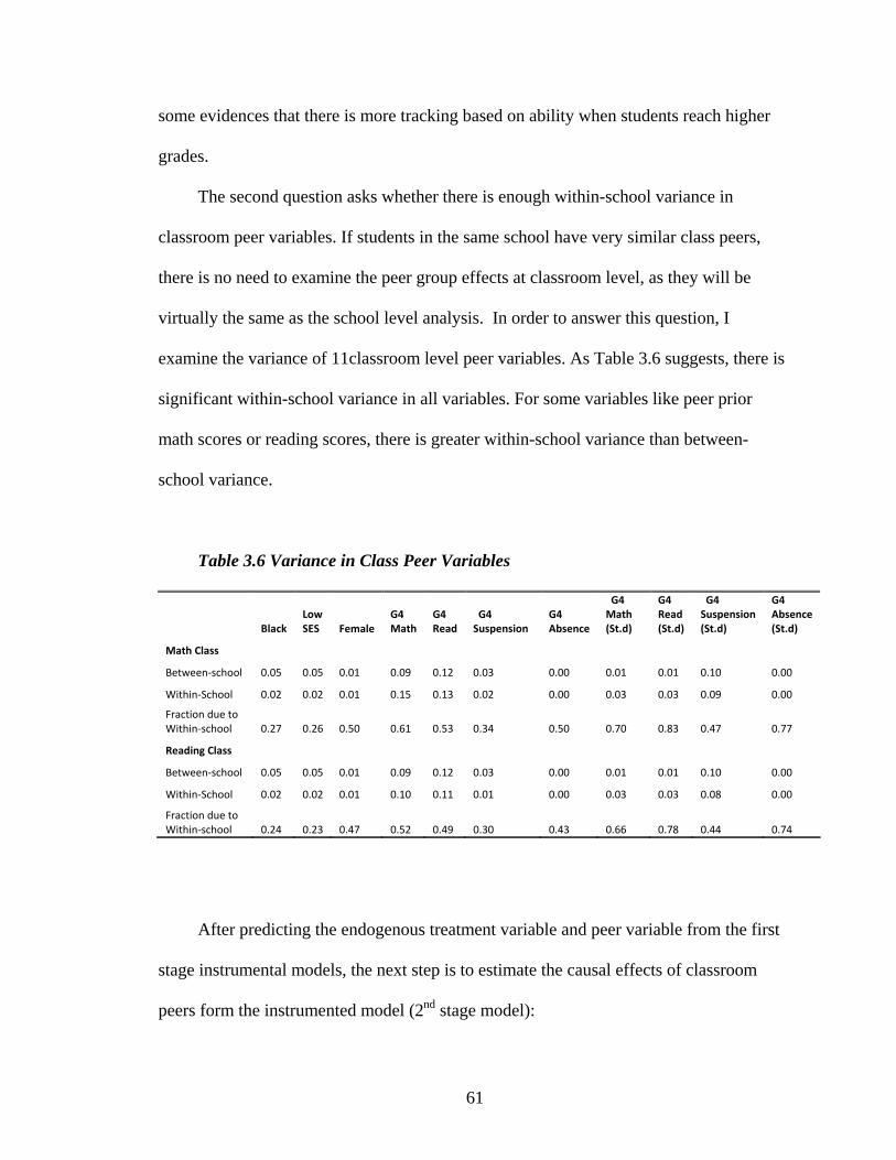
61

some evidences that there is more tracking based on ability when students reach higher

grades.

The second question asks whether there is enough within-school variance in

classroom peer variables. If students in the same school have very similar class peers,

there is no need to examine the peer group effects at classroom level, as they will be

virtually the same as the school level analysis. In order to answer this question, I

examine the variance of 11classroom level peer variables. As Table 3.6 suggests, there is

significant within-school variance in all variables. For some variables like peer prior

math scores or reading scores, there is greater within-school variance than between-

school variance.

Table 3.6 Variance in Class Peer Variables

Black

Low SES Female

G4 Math

G4 Read

G4 Suspension

G4 Absence

G4 Math (St.d)

G4 Read (St.d)

G4 Suspension (St.d)

G4 Absence (St.d)

Math Class

Between‐school 0.05 0.05 0.01 0.09 0.12 0.03 0.00 0.01 0.01 0.10 0.00

Within‐School 0.02 0.02 0.01 0.15 0.13 0.02 0.00 0.03 0.03 0.09 0.00

Fraction due to Within‐school 0.27 0.26 0.50 0.61 0.53 0.34 0.50 0.70 0.83 0.47 0.77

Reading Class

Between‐school 0.05 0.05 0.01 0.09 0.12 0.03 0.00 0.01 0.01 0.10 0.00

Within‐School 0.02 0.02 0.01 0.10 0.11 0.01 0.00 0.03 0.03 0.08 0.00

Fraction due to Within‐school 0.24 0.23 0.47 0.52 0.49 0.30 0.43 0.66 0.78 0.44 0.74

After predicting the endogenous treatment variable and peer variable from the first

stage instrumental models, the next step is to estimate the causal effects of classroom

peers form the instrumented model (2nd stage model):

62

cijiiNcijiicij vdPPdXY ˆˆˆˆ)( (3.18)

where id̂ and cijP̂ are instrumented treatment indicator and peer variables, and NP̂ is an

predicted neighborhood school peer variable that is included to remove residential

location selectivity. Model (3.18) eliminates the endogeneity in classroom peer

composition by exploiting randomly determined lottery outcomes to construct

instruments.

The estimation of classroom level peer effects deals with all other complications

following the steps in the school level investigation. One thing should be emphasized is

that classroom level peer effect estimation faces more severe omitted variable biases. For

example, if the majority of students in a classroom are above the average academic level

(measured by prior achievement) and all high quality students are assigned to the best

teachers, then failure to account for teacher characteristics will falsely attribute the

teacher’s contribution to peer influences, which will bias the peer effect estimation

upwardly. Fortunately, I can use the course data to match each student to the class

instructor for both math and reading courses, and therefore to control for teacher fixed

effect cT in the model:

cijciiNcijiicij vTdPPdXY )( (3.18)

With cT included in the model, teacher’s influence on student achievement no longer

enters through the error term, which reduces the omitted variable bias.

3. Peer Effects on Non-Academic Outcomes

In this study, the district administrative data sets provide student attendance records

and discipline records, which enables me to derive two non-academic outcome variables:

63

the first one is attendance, measured by student absence rate (absent days/ total

enrollment days) in each school year; the second one is disciplinary infraction, presented

by the year-total times of suspension that a student was given as consequences to his/her

misconduct at school.

The two behavioral outcome variables, attendance and disciplinary infractions, are

important indicators for student participation and engagement in schools (Rowley, 2005).

They are also significant factors associated with student educational attainment. Research

has found that students with higher attendance rate are more likely to have better

academic achievement (Anderson, Christenson, Sinclair, and Lehr, 2004; and Lamdin,

1995) and less likely to drop out from school (Alexander, Entwisle, & Horsey, 1997;

Rumberger, 1995). Similarly, students with frequent misconduct have been found

significantly associated with low academic achievement (Finn & Rock, 1997; Wentzel,

Weinberger, Ford, & Feldman, 1990; Wentzel, 1993) and high drop-out rate (Rumberger,

1995).

The estimation of peer effects on behavioral outcomes at both school and classroom

levels will follow the same strategies described in above sections; but the dependent

variable in the two models (3.13) and (3.17) are now replaced by the attendance or

delinquency outcomes for student i.

4. The Impact of Peer Composition Heterogeneity

In addition to examining the influences from average peer group qualities on student

outcomes, this study also intends to investigate the impacts from the dispersion of peer

characteristics. For example, do students benefit more from an ability-tracking class or

from a homogeneous class?

64

Previous studies have mixed conclusions on the influences of heterogeneity in peer

composition. In the Texas study, Hanushek and colleagues (2003) find no impacts from

the dispersion in school level peer achievement. Fertig (2003), however, provides some

evidences that heterogeneous peer academic ability composition at school level detriment

individual student reading achievement. Kang’s study (2007) on Korean schools reveals

that weak students are negatively impacted by the dispersion of peer qualities within

classroom, while strong students are positively impacted by the dispersion.

This project will examine the relationship between the dispersion of peer composition

and student outcomes at both school and classroom level. The dispersion of peer

composition is measured by the standard deviation in four major peer variables: prior

math scores, prior reading scores, prior absence rate, and prior disciplinary infractions.

The analytical strategies are very similar to those used for estimating average peer effects

except that the regression model includes both the mean peer variable and the standard

deviation of the peer variable:

iNiiNiNiMiNMiiij vdPdPdstdPdstdPPdXY )()]1)((.)(.[][)(

(3.19)

iNiiNcijcijiicij vdPPdstPdXY )(.)( (3.20)

5. Heterogeneous Peer Effects

Although the existence and magnitude of peer effects would be significant findings,

another important objective of this project is to examine whether peer qualities impact a

particular student group more significantly than other groups depending on student’s own

characteristics such as gender, race, or initial position in achievement distribution. That is

to answer the second research question “to whom do peer effects matter the most?”.

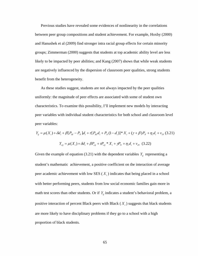
65

Previous studies have revealed some evidences of nonlinearity in the correlations

between peer group compositions and student achievement. For example, Hoxby (2000)

and Hanushek et al (2009) find stronger intra racial group effects for certain minority

groups; Zimmerman (2000) suggests that students at top academic ability level are less

likely to be impacted by peer abilities; and Kang (2007) shows that while weak students

are negatively influenced by the dispersion of classroom peer qualities, strong students

benefit from the heterogeneity.

As these studies suggest, students are not always impacted by the peer qualities

uniformly: the magnitude of peer effects are associated with some of student own

characteristics. To examine this possibility, I’ll implement new models by interacting

peer variables with individual student characteristics for both school and classroom level

peer variables:

iNiiNiiNiMiNMiiij vdPXdPdPdPPdXY )(*)]1([][)( (3.21)

iNiiNicijcijiicij vdPXPPdXY *)( (3.22)

Given the example of equation (3.21) with the dependent variables ijY representing a

student’s mathematic achievement, a positive coefficient on the interaction of average

peer academic achievement with low SES ( iX ) indicates that being placed in a school

with better performing peers, students from low social economic families gain more in

math test scores than other students. Or if ijY indicates a student’s behavioral problem, a

positive interaction of percent Black peers with Black ( iX ) suggests that black students

are more likely to have disciplinary problems if they go to a school with a high

proportion of black students.

66

CHAPTER IV

PEER EFFECTS ON ACADEMIC ACHIEVEMENT ---RESULTS FROM SCHOOL LEVEL ANALYSIS

This study is part of a big project investigating magnet school impacts and peer

effects on student achievement. While the first part study on magnet school effect aims to

answer the question whether students in magnet schools perform better than their

counterparties in neighborhood schools, this dissertation intends to find out if peer effects

play a significant role influencing student outcomes.

This chapter reports the findings of school level peer group impacts on student

academic achievement. The first section presents descriptive statistics, including lottery

participant characteristics, school level peer characteristics, and student achievement in

math and reading. The second section reports the regression results on magnet school

treatment effects, wherein the regressor of interest is only the treatment indicator id and

no peer variables are included. The purpose of presenting the findings from the treatment

effect models is to provide a baseline for further peer effect investigation, which

examines to what extent the magnet effects are attributable to its peer composition. The

subsequent sections report and discuss the findings as they are related to the following

questions:

How do average school level peer characteristics impact student academic

achievement in math and reading?

How does the variance of school peer characteristics influence student

achievement?

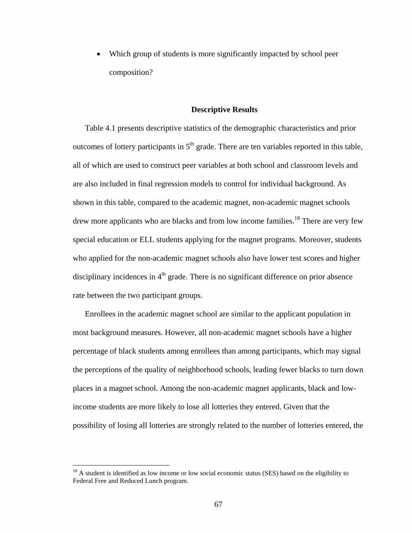
67

Which group of students is more significantly impacted by school peer

composition?

Descriptive Results

Table 4.1 presents descriptive statistics of the demographic characteristics and prior

outcomes of lottery participants in 5th grade. There are ten variables reported in this table,

all of which are used to construct peer variables at both school and classroom levels and

are also included in final regression models to control for individual background. As

shown in this table, compared to the academic magnet, non-academic magnet schools

drew more applicants who are blacks and from low income families.18 There are very few

special education or ELL students applying for the magnet programs. Moreover, students

who applied for the non-academic magnet schools also have lower test scores and higher

disciplinary incidences in 4th grade. There is no significant difference on prior absence

rate between the two participant groups.

Enrollees in the academic magnet school are similar to the applicant population in

most background measures. However, all non-academic magnet schools have a higher

percentage of black students among enrollees than among participants, which may signal

the perceptions of the quality of neighborhood schools, leading fewer blacks to turn down

places in a magnet school. Among the non-academic magnet applicants, black and low-

income students are more likely to lose all lotteries they entered. Given that the

possibility of losing all lotteries are strongly related to the number of lotteries entered, the

18 A student is identified as low income or low social economic status (SES) based on the eligibility to Federal Free and Reduced Lunch program.

68

higher percentage of black/low-income students losing all lotteries reflects more about

the application behavior than the fairness of the lotteries.19

Table 4.2 presents school peer characteristics for lottery participants in 5th grade.

School/grade level peer variables are calculated by averaging over all students in each

grade in the schools attended. For students who switched schools during the school year,

the peer variables are weighted averages reflecting the proportion of school days spent in

each school. A student is defined as a magnet school enrollee if his/her end-of-year

(EOY) school is recorded as a magnet school.20

For all lottery participants, the peer characteristics for the enrollees are of differences

from the general applicants. Students who attend the academic magnet school have more

favorable peers than the applicants over almost all dimensions. However, Compared to

the general participants in non-academic magnets, enrollees in these schools are more

likely to have black and low SES peers and peers with lower prior test scores. All magnet

school enrollees have lower percentage of peers identified as special education or ELL

students. Because the enrollees for each magnet program attend the same school, the

standard deviations of all peer variables are much lower. Since the sample included in

Table 4.2 is pooled across all five cohorts of 5th graders, the non-zero standard deviation

reflects the variation from one cohort to the next. The big difference between peer

characteristics for enrollees and lottery losers suggests that the qualities of one student’s

peers are very much affected by the lottery outcomes.

19 Among all the entrants to the non-academic magnet lotteries, 59% Blacks applied for at least 2 schools, while 75% non-black students applied for 2 schools or more. Similarly, 59% low income students and 71 non low income students applied for multiple lotteries. 20 A student may attend a non magnet school at the beginning of the school year, but receive the notice during the school year and switched to the magnet school then.

69

Table 4.1 Lottery Participant Characteristics

Black Low Income

Special Education ELL Female Hispanic G4 Math G4 Reading G4 Suspension G4 Absence

Pct Pct Pct Pct Pct Pct Mean SD Mean SD Mean SD Mean SD

Academic

Academic

Participants1 20.6 14.8 1.1 0.9 53.1 1.1 1.13 0.68 1.22 0.68 0.03 0.20 0.03 0.03

Losing Participants2 22.1 15.5 1.0 1.0 49.9 1.1 1.11 0.68 1.20 0.68 0.02 0.19 0.03 0.03

Losing Participants3 17.7 13.6 1.2 1 49.9 1.2 1.13 0.68 1.20 0.70 0.02 0.19 0.03 0.03

Enrolling Participants4 20.6 12.0 0.1 0.1 53.8 1.3 1.15 0.67 1.23 0.66 0.03 0.22 0.03 0.03

Non‐Academic

North

Participants1 51.3 34 4.3 0.4 60.2 1.5 0.43 0.83 0.53 0.85 0.08 0.39 0.03 0.03


Losing Participants3 72.2 53.7 3.7 0 62.9 0 0.09 0.90 0.21 0.72 0.19 0.62 0.04 0.04


South

Participants1 42.6 24.9 2.5 1.7 46.4 1 0.75 0.83 0.76 0.82 0.07 0.38 0.03 0.03


Losing Participants3 47.7 27 4.5 2.7 40.5 1.8 0.73 0.79 0.76 0.71 0.07 0.37 0.03 0.03

Enrolling Participants4 49.2 21.4 1.6 3.1 44.8 1 0.69 0.79 0.66 0.75 0.05 0.35 0.02 0.03

East

Participants1 43.6 30.7 2.6 1 54.7 1.1 0.63 0.83 0.74 0.85 0.05 0.32 0.03 0.03




West

Participants1 63 36 5.9 1 51.9 1.4 0.36 0.80 0.49 0.86 0.07 0.33 0.03 0.03


Losing Participants3 77.8 61.1 0 0 44.4 0 0.35 0.55 0.39 0.63 0.22 0.55 0.03 0.03

Enrolling Participants4 93.3 40 6.6 0 60 0 ‐0.08 0.69 0.05 0.64 0.00 0.00 0.03 0.02

70

Table 4.1 Continued

Composite Non‐Academic

Participants1 45.4 29.4 3.2 1.2 52.5 1.2 0.60 0.84 0.67 0.84 0.06 0.37 0.03 0.03




1.Counted as 4th graders who participated the magnet school lottery and had non‐missing test scores in 4th grade.

2. Students who lost this lottery (neither outright winner nor delayed winner by the start of 5th grade).

3. Students who lost all lotteries they entered (neither an outright winner nor a delayed winner by the start of 5th grade).

4.Counted only 5th graders who enrolled in the magnet school and have non‐missing test scores in 4th and 5th grades.

71

Table 4.2 School Peer Characteristics in Grade 5 1

Black Low Income Special Education ELL Female Hispanic G4 Math G4 Reading G4Suspension G4 Absence

Mean SD Mean SD Mean SD Mean SD Mean SD Mean SD Mean SD Mean SD Mean SD Mean SD

Academic pct pct pct pct pct pct

Academic

Participants 35.8 18.5 30.1 19.3 6.7 6.8 2.1 3.3 51.3 4.7 2.7 3.9 0.56 0.54 0.61 0.56 0.09 0.10 0.03 0.01

Enrollees 20.5 3.7 12.0 2.9 0.5 0.6 0.1 0.2 54.2 2.0 1.3 0.7 1.16 0.08 1.23 0.06 0.03 0.01 0.03 0.00

Losers2 41.5 16.2 43.1 17.8 13.1 4.8 4.2 4.2 48.4 4.5 4.7 5.3 0.08 0.26 0.11 0.31 0.14 0.13 0.04 0.01

Non‐Academic North

Participants 56.3 21 44.3 17.4 8.7 5.9 1.9 3 52.8 5.5 2.5 3.7 0.20 0.42 0.45 0.43 0.14 0.10 0.03 0.01

Enrollees 73.1 5.4 51.2 7.4 8.9 4.5 0.3 0.2 57.7 4 1.3 1 ‐0.02 0.11 0.08 0.11 0.18 0.04 0.04 0.00

Losers2 59.8 20.9 50.3 19.1 10.7 4.6 3.7 4.9 49.8 4 3.5 4.8 0.05 0.36 0.08 0.40 0.15 0.10 0.04 0.01

South

Participants 49.9 20.6 39.1 17.3 7.2 5.9 2.3 2.9 50.6 4.5 2.3 2.9 0.37 0.45 0.40 0.47 0.12 0.10 0.03 0.01

Enrollees 61.4 1.6 44 7.3 6.2 4.1 2.8 1.5 48.6 2.3 1.2 0.4 0.32 0.16 0.29 0.18 0.13 0.08 0.03 0.00

Losers2 51.4 21.9 43.3 17.9 11.7 5.5 3.7 3.7 48.8 3.5 3.4 4.6 0.10 0.32 0.12 0.36 0.15 0.09 0.04 0.01

East

Participants 50.4 20.2 40.1 18.8 7.2 6.5 2 2.9 51.6 4.8 2.3 3.5 0.36 0.46 0.40 0.48 0.11 0.11 0.03 0.01

Enrollees 52.9 6.4 33.3 5 1.7 1.6 0.9 1 53.2 3.6 0.7 0.6 0.57 0.10 0.65 0.09 0.04 0.01 0.03 0.01

Losers2 59.2 21.5 53.2 20.2 12.9 5.9 2.4 2.7 50.2 4.3 2.8 2.8 ‐0.00 0.31 0.01 0.33 0.18 0.14 0.04 0.01

West

Participants 59.4 22.5 45.6 16.6 7.8 5.5 1.8 3 51.1 5.1 2.7 3.9 0.27 0.41 0.30 0.45 0.10 0.08 0.03 0.01

Enrollees 95.2 0 54.2 0 9.5 0 0 0 55 0 1.7 0 ‐0.05 0.00 ‐0.05 0.00 0.11 0.00 0.03 0.00

Losers2 61.3 20.7 61.3 18.6 12.3 4.6 3.4 4 50.4 3.7 3.4 4.7 ‐0.03 0.41 ‐0.02 0.44 0.19 0.12 0.04 0.00


Participants 52.2 21.5 41.2 18.2 7.8 6.2 2 2.9 51.6 5 2.4 3.5 0.30 0.45 0.34 0.47 0.12 0.10 0.03 0.01

Enrollees 64.7 10.5 44.4 9.7 6.3 4.7 1.4 1.5 53.2 5.1 1.13 0.8 0.24 0.27 0.29 0.26 0.13 0.08 0.03 0.01

Losers2 55.7 21.5 49.2 19.7 12.4 5.4 3.3 3.8 49.4 3.9 3.4 4.3 0.03 0.31 0.05 0.34 0.17 0.11 0.04 0.01

1.Counted as 5th graders with non‐missing test scores in both grades 4 and 5.

2. Students who lost all lotteries (neither as outright winner nor delayed winner by the start of 5th grade).

Sample limited to 4th graders with non‐missing test scores.

72

There are some discrepancies between Table 4.1 and 4.2, notably for the non-

academic magnet schools. Overall, the percentage of black peers or low SES peers is

higher than the percentage of black or low SES lottery participants enrolling in the non-

academic magnet schools. As noted before, many non-academic magnet schools have

places filled by students from other channels such as geographic priority zones, sibling

preference, or a feeder school, which causes school peer characteristics to differ from the

characteristics of lottery participants.

Table 4.3 presents the descriptive statistics on the two dependent variables --- student

test scores in math and reading. As I mentioned in Chapter III, I standardized student test

scores by grade and year: for every grade (from grade 4 to grade 8) in each school year

from 1999 to 2007, the district mean score is 0 with a standard deviation of 1. As shown

in Table 4.3, overall, lottery participants score higher in both math and reading than other

middle school students in the district. Academic magnet school enrollees appear to

perform better in both subjects than the lottery losers who enrolled in other schools. Also,

the standardized scores for the academic magnet enrollees are less dispersed than the

scores for lottery losers enrolled in neighborhood schools. The non-academic composite

enrollees, however, only significantly outperform their counterpart students in

neighborhood schools in 6th grade; the achievement differences between the enrollees and

lottery losers are not notable in other grades.

73

Table 4.3 Descriptive Statistics on Academic Achievement Grade 5 Grade 6 Grade 7 Grade 8

Math Scores Mean SD Mean SD Mean SD Mean SD

Lottery Participants

All 0.82 0.86 0.86 0.85 0.86 0.84 0.86 0.85

Academic

Participants 1.22 0.70 1.21 0.75 1.23 0.72 1.22 0.71

Enrollees 1.33 0.65 1.28 0.73 1.32 0.69 1.36 0.65

Enrollees in Other Magnet Schools 1.09 0.70 1.23 0.74 1.19 0.70 1.19 0.76

Enrollees in Non‐Magnet Schools 1.17 0.73 1.15 0.75 1.16 0.75 1.12 0.73


Participants 0.62 0.85 0.69 0.85 0.69 0.84 0.70 0.87

Enrollees 0.49 0.81 0.66 0.82 0.60 0.81 0.63 0.86



Reading Scores Mean SD Mean SD Mean SD Mean SD


All 0.89 0.81 0.89 0.84 0.90 0.84 0.87 0.82

Academic

Participants 1.26 0.67 1.26 0.72 1.28 0.71 1.22 0.69

Enrollees 1.35 0.63 1.33 0.69 1.45 0.67 1.38 0.63




Participants 0.71 0.81 0.73 0.84 0.73 0.86 0.70 0.81

Enrollees 0.60 0.76 0.65 0.78 0.59 0.74 0.58 0.72



*Count only students who have non‐missing 4th grade test scores.

Magnet School Treatment Effects

The estimation of magnet school treatment effects follows the same strategy as the

peer effect estimation except that the peer term is dropped from the model. Because there

are two treatment groups (the academic magnet, and the composite non-academic

magnet) in the data, the regressors of interest include two treatment indicators: 1id equals

1 if student i enrolled in the academic magnet; 2id equals 1 if student i enrolled in the

74

non-academic composite. The regression model estimating magnet school treatment

effects is expressed as

iNiiiiiiiij uddddXY 22112211)( (4.1)

In order to eliminate the possible selection bias arising from non-compliances, lottery

outcomes are exploited to form the instruments for both treatment indicators 1id and 2id .

Table 4.4 reports the estimates of magnet treatment effect models on student achievement

in math and reading. For both subjects, I ran the regression models on two different

samples separately21: students in the first two grades (Grades 5 and 6), and students in all

four grades (Grades 5 to 8). The point estimates of treatment indicators suggest that the

academic magnet school improves student standard score by almost 0.1 point of

standardized scores in both math and reading. This implies that students enrolling in the

academic magnet school achieve 0.1 point higher in standardized score than the test

scores they would achieve if they had lost the academic magnet lottery and enrolled in

the neighborhood schools. The estimates of treatment effects for the non-academic

magnet composite are not statistically significant in either subject.

21 As mentioned in Chapter III, the purpose of limiting the investigation to 5th and 6th graders is to avoid the complications arising from the presence of the second academic magnet school in later grades. I also ran a set of grade-specific models, wherein the treatment indicator is interacted with grade indicators (for grades 6 to 8) to examine whether the treatment effect varies across grades. Since the treatment effects in grades 6 to 8 are not found different from 5th grade, I’m not going to report the results from the grade specific models in the text.

75

Table 4.4 Magnet School Treatment Effects on Academic Achievement

Math Reading

Independent Variables First 2 grades

All 4 grades

First 2 grades

All 4 grades

Academic Magnet Treatment

Academic 0.09* 0.08* 0.07* 0.09**

(0.04) (0.03) (0.03) (0.03)

Non‐Academic Magnet Treatment

Composite 0.11 0.07 0.02 ‐0.01

(0.08) (0.08) (0.08) (0.07)

Student Characteristics

Black ‐0.19*** ‐0.20*** ‐0.17*** ‐0.17***

(0.02) (0.02) (0.02) (0.01)

Hispanic ‐0.24*** ‐0.12* 0.01 0.02

(0.07) (0.05) (0.06) (0.05)

Special Education ‐0.20*** ‐0.17*** ‐0.12** ‐0.11***

(0.05) (0.03) (0.04) (0.03)

Low SES ‐0.09*** ‐0.12*** ‐0.12*** ‐0.14***

(0.02) (0.01) (0.02) (0.01)

ELL 0.17 0.16* ‐0.10 ‐0.11

(0.09) (0.07) (0.08) (0.07)

Female ‐0.03 ‐0.03** 0.01 0.04***

(0.01) (0.01) (0.01) (0.01)

Grade 4 Reading 0.18*** 0.18*** 0.53*** 0.50***

(0.01) (0.01) (0.01) (0.01)

Grade 4 Math 0.44*** 0.43*** 0.11*** 0.12***

(0.01) (0.01) (0.01) (0.01)

Grade 4 Absence ‐0.86** ‐1.19*** ‐0.31 ‐0.44*

(0.29) (0.21) (0.26) (0.20)

Grade 4 Suspension 0.00 0.00 0.01 ‐0.01

(0.02) (0.02) (0.02) (0.02)

Over‐Identification Test 0.61 0.57 0.75 0.82

N 6267 11869 6270 11885

* p<0.05, ** p<0.01, *** p<0.001

The other coefficients reported in Table 4.4 pertain to student characteristics. Black

students and students from low SES families score significantly below other lottery

participants in both mathematics and reading. This is also true of special education

students in both subjects. Although Hispanic students score significantly lower in math,

their reading achievement does not differ from other students. ELL students in our

76

sample outperform other students by 0.16 standard scores in mathematics22, but not in

reading. As one would expect, prior achievement is significantly associated with later

performance, with a more substantial intra-subject correlation. For example, a 0.5 point

increase in 4th grade standardized math score is related to 0.2 point of standardized score

increase in middle school math test. Moreover, students with a high absence rate in 4th

grade have lower achievement in middle school grades, while prior disciplinary

infractions are not found significantly related to middle school performance.

The P-values of the omnibus over-identification tests are reported in the second panel

of the table.23 The results indicate that the instruments used in all four models are

exogenous.

Impacts of Average School Peer Characteristics

This section investigates the average school level peer effects on middle student

achievement in both math and reading. All ten specifications of peer characteristics

(including 6 predetermined peer characteristics, and 4 lagged values of peer outcome

measures) are examined. First, I run a set of single variable models with only one peer

variable included in the regression; I then include all specifications of peer characteristics

in one regression. Coefficients from all 11 models are reported in this part. Similar to the

treatment effect investigation, all models are run twice using both the small sample

comprising grades 5 and 6 and the big sample of all four grades. Overall, the findings

from both samples are close, but the estimates from the models using the big sample have

22 In the regression sample, 164 (1.25%) observations are Hispanic and 79 (0.6%) observations are ELL students, but only 9 Hispanic observations are identified as ELL students. 23 Recall that the lottery outcomes are not binary, and there are two excluded instruments (outright-win and delayed-win) for each treatment variable. Therefore, the validity of the external instruments is tested for all regression models using the over-identification tests.

77

smaller standard errors and higher P-values from the omnibus over-identification tests.

Therefore, I’m only going to report and discuss the results from the full sample analysis.

Math Achievement

Estimates of average school level peer effects on math achievement are presented in

Table 4.5. As introduced in Chapter III, there are two types of peer variables included in

the model: the exogenous, lottery-based variation in peer characteristics

)]1([ iNiM dPdP ; and the endogenous, residence-based variation in peer

characteristicsNP . The causal relationship between peer group composition and student

outcomes are obtained from the estimates on the first exogenous peer term; and the

second peer term is included to control for residence choice (or neighborhood school

choice). The estimated effects of both peer terms are reported in Table 4.5 along with the

magnet school treatment effects. Individual characteristics are also controlled in the

regression models, but are not reported in the table since the estimates are quite similar to

those in previous treatment effect models.

Several estimates from Table 4.5 are noteworthy. The first result to draw is from

model 1, which suggests that students tend to perform worse in mathematics if they are in

a school with a high proportion of black students. The estimate of this racial composition

effect is quite large. For instance, increasing the share of black schoolmates from 25% to

75% would reduce student math scores by 0.25 points of standardized score. Although

the estimate of percent low SES student effect is not statistically significant (Model 2),

the coefficient on this variable is negative. Also note that in model 1 and model 2,

including the peer variables --- percent Black and percent low income students ---

78

completely overturns the positive treatment effect from the academic magnet school

reported in Table 4.4. This implies that if the academic magnet school lottery losers

attend a neighborhood school where peer racial or Social Economic Status composition is

very similar to the academic magnet school, they would do as well in mathematics as

those students enrolled in the academic magnet.

The second significant estimate is on school gender composition effect (Model 3),

which shows that having more girls in a school decreases average math scores for the

lottery participants. While some previous studies find female peers help to improve

student achievement (e.g., Hoxby, 2000; Lavy & Scholosser, 2007), results in Table 4.5

do not support that conclusion. The coefficient is strikingly large --- for 50 percent point

increase of female students in the school, the average math score falls by almost 0.8

standard deviations. However, a 50% change in percent school female population far

exceeds anything observed in our data.

Model 5 and Model 6 find significant and positive coefficients on school percent

special education students and school percent ELL students. For example, the estimate

from Model 5 suggests that double the special education population in the academic

magnet school (from 0.5% to 1%) would increase the average math scores by 0.02 points

of standardized scores. However, although the school level estimates suggests positive

peer effect from percent special education or ELL students, the impact of having special

education peers or ELL peers is more likely to work through the classroom. For instance,

a teacher may spend disproportional time on a leaning disabled student, which would

have a great impact on the children in the same classroom but not on other children in the

school. Therefore, it would be more meaningful to draw the conclusion on the effect of

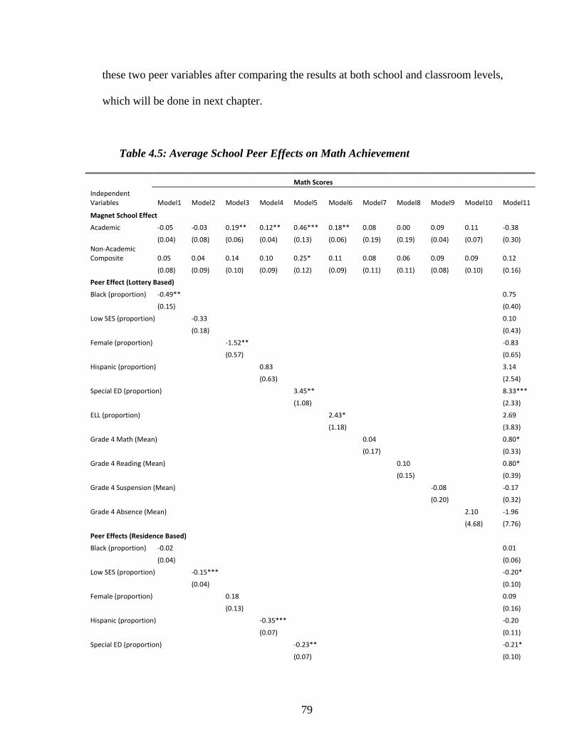
79

these two peer variables after comparing the results at both school and classroom levels,

which will be done in next chapter.

Table 4.5: Average School Peer Effects on Math Achievement

Math Scores

Independent Variables Model1 Model2 Model3 Model4 Model5 Model6 Model7 Model8 Model9 Model10 Model11

Magnet School Effect

Academic ‐0.05 ‐0.03 0.19** 0.12** 0.46*** 0.18** 0.08 0.00 0.09 0.11 ‐0.38

(0.04) (0.08) (0.06) (0.04) (0.13) (0.06) (0.19) (0.19) (0.04) (0.07) (0.30) Non‐Academic Composite 0.05 0.04 0.14 0.10 0.25* 0.11 0.08 0.06 0.09 0.09 0.12

(0.08) (0.09) (0.10) (0.09) (0.12) (0.09) (0.11) (0.11) (0.08) (0.10) (0.16)

Peer Effect (Lottery Based)

Black (proportion) ‐0.49** 0.75

(0.15) (0.40)

Low SES (proportion) ‐0.33 0.10

(0.18) (0.43)

Female (proportion) ‐1.52** ‐0.83

(0.57) (0.65)

Hispanic (proportion) 0.83 3.14

(0.63) (2.54)

Special ED (proportion) 3.45** 8.33***

(1.08) (2.33)

ELL (proportion) 2.43* 2.69

(1.18) (3.83)

Grade 4 Math (Mean) 0.04 0.80*

(0.17) (0.33)

Grade 4 Reading (Mean) 0.10 0.80*

(0.15) (0.39)

Grade 4 Suspension (Mean) ‐0.08 ‐0.17

(0.20) (0.32)

Grade 4 Absence (Mean) 2.10 ‐1.96

(4.68) (7.76)

Peer Effects (Residence Based)

Black (proportion) ‐0.02 0.01

(0.04) (0.06)

Low SES (proportion) ‐0.15*** ‐0.20*

(0.04) (0.10)

Female (proportion) 0.18 0.09

(0.13) (0.16)

Hispanic (proportion) ‐0.35*** ‐0.20

(0.07) (0.11)

Special ED (proportion) ‐0.23** ‐0.21*

(0.07) (0.10)

80

Table 4.5 (Continued) ELL (proportion) ‐0.24*** ‐0.04

(0.06) (0.08)

Grade 4 Math (Mean) 0.04* ‐0.26*

(0.02) (0.10)

Grade 4 Reading (Mean) 0.05* 0.18

(0.02) (0.10)

Grade 4 Suspension (Mean) ‐0.08 0.11

(0.06) (0.08)

Grade 4 Absence (Mean) ‐2.53* 0.94

(1.00) (1.52)


Yes Yes Yes Yes Yes Yes Yes Yes Yes Yes Yes

Over‐identification Test 0.6 0.53 0.71 0.8 0.45 0.34 0.58 0.58 0.81 0.57 0.96

Sample Size24 11780 11780 11780 11780 11780 11780 11778 11778 11778 11778 11778

* p<0.05, ** p<0.01, *** p<0.001

School level models do not find significant estimates of average peer achievement

variables (Models 7 and 8), average peer disciplinary infractions (Model 9)25, or average

peer absence rate (Model10). Because middle school students (especially students in later

grades) are often grouped for instruction based on their academic abilities26 --- students

with lower prior achievement (or behavioral problems) are often placed in a class with

other disadvantaged students, it is possible that average school level peer academic

ability or behavioral measures may only have a moderate or no impact on these variables.

24 The regression sample is limited to lottery participants to all magnet middle schools. The sample size in the peer effect models is 11780, which is smaller than the sample size in the treatment effect models (11885) in Table 4.4. The difference is caused by the creation of peer variables --- there are about 100 observations whose End-of-Year school can not be identified. 25 In order to circumvent the reflection problems, I use student 4th grade test scores and behavioral records to construct these peer variables. Given that students in elementary schools are less likely get suspension, I also constructed another peer disciplinary variable representing average 4th grade punishment numbers including severe punishments such as suspension and other less severe punishments. However, the conclusion from the average punishment peer variable is very similar to that from the suspension variable except that the coefficient is smaller. Since suspension is more often used in other studies measuring student disciplinary infractions (e.g., Figlio, 2005; Rowley, 2005), I follow the literature and keep only the suspension variable in the result table. 26 It is also possible that some schools keep students with behavioral problems in one class just because the teacher is more experienced with disruptive students.

81

Note that although there is no significant peer effect from these four peer variables, the

positive treatment effect of the academic magnet program vanishes in all four models

while the peer variables are controlled. Because of the tracking police in middle school,

the influence of peer achievement or misconduct is more likely to work through a

classroom rather than through the school/grade level; therefore, I expect significant

estimates of peer ability effects at the classroom level. This of course will be examined in

next chapter.

Model 11 incorporates all peer variables in one regression. Among the four peer

variables that are found significantly influencing student math achievement in the single

variable models, only the estimate of percent special education peers remains significant

and positive. With all specifications of peer characteristics controlled in one model, the

estimates of prior peer math and reading scores become weakly significant (P<0.05) and

show positive impact on student math achievement. Due to the correlations among the

peer variables, the estimates of most peer characteristics are insignificant in the full

model. Moreover, with all peer variables controlled in the same equation, the coefficient

on the academic magnet school treatment effect turns to -0.38. This result suggests that if

school peer compositions are held constant, lottery winners enrolling in the magnet

schools do not perform better than their counterpart students enrolling in neighborhood

schools, at least not in math test.

The lower part of Table 4.6 presents the estimates on the residence based peer

variables. Four residence-based pre-determined (contextual) peer characteristics, percent

low SES students, percent Hispanic students, percent special education students, and

percent ELL students, have shown negative impacts on student math achievement in

82

middle school; the estimates on the two residence-based peer ability variables (Model 7

and Model 8) suggest that students tend to score slightly higher in math if their

neighborhood schools have more high performing students. The residence-based peer

absence rate is also found reducing student achievement. However, compared to the

estimated effects from the exogenous, lottery-based peer variables, the estimates of

residence based peer characteristic effects are smaller in magnitude.

The findings from the residence-based peer variables suggest that although the

admission lotteries randomly assign students between a magnet school and a

neighborhood school, family residential choice (indicated by neighborhood school

characteristics) is still correlated with some factors influencing student achievement ---

although the correlation is smaller than the peer effects identified from the exogenous

peer characteristics.

Reading Achievement

Estimates of peer effect models on reading achievement are presented in Table 4.6.

Compared to the estimates from the math achievement models, there are fewer significant

peer variable coefficients on reading achievement. The first significant estimate is percent

ELL students, which shows positive impact on student reading achievement in middle

school. Surprisingly, Model 6 suggests that school level average peer reading

achievement reducing student reading scores in middle school: if average school peer 4th

grade reading scores increase by 1 point of standardized scores, student reading

achievement in middle school falls by almost 0.3 points of standardized scores. The last

83

significant coefficient is from model 10, which finds a positive association between

individual reading achievement and prior peer absence rate.

Table 4.6: Average School Peer Effects on Reading Achievement

Reading Scores



Academic 0.04 0.12 0.15** 0.13*** 0.28* 0.21*** 0.41* 0.44* 0.06 0.21*** 0.53

(0.04) (0.07) (0.06) (0.04) (0.12) (0.05) (0.18) (0.18) (0.04) (0.06) (0.27) Non‐Academic Composite ‐0.02 0.01 0.03 0.03 0.09 0.05 0.07 0.09 ‐0.03 0.10 0.25

(0.07) (0.08) (0.09) (0.08) (0.11) (0.08) (0.10) (0.11) (0.08) (0.10) (0.14)

Peer Effect (Lottery Based) Black (proportion) ‐0.20 0.21

(0.14) (0.37)

Low SES (proportion) 0.05 ‐0.54

(0.17) (0.38)

Female (proportion) ‐0.88 ‐1.23*

(0.54) (0.57)

Hispanic (proportion) 0.90 ‐1.70

(0.59) (2.25)

Special ED (proportion) 1.72 1.69

(1.01) (2.14)

ELL (proportion) 3.18** 5.70

(1.13) (3.45)

Grade 4 Math (Mean) ‐0.29 ‐0.04

(0.16) (0.30)

Grade 4 Reading (Mean) ‐0.29* ‐0.02

(0.14) (0.36)

Grade 4 Suspension (Mean) ‐0.27 ‐0.64*

(0.18) (0.29)

Grade 4 Absence (Mean) 12.20** 14.38*

(4.45) (7.03)

Peer Effects (Residence Based) Black (proportion) ‐0.06 ‐0.04

(0.04) (0.06)

Low SES (proportion) ‐0.18*** ‐0.08

(0.04) (0.09)

Female (proportion) ‐0.03 ‐0.09

(0.12) (0.14)

Hispanic (proportion) ‐0.32*** ‐0.25**

(0.07) (0.10)

Special ED (proportion) ‐0.16* ‐0.03

(0.07) (0.09)

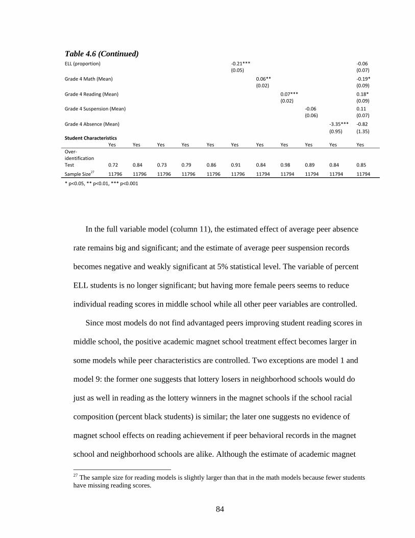
84

Table 4.6 (Continued)

ELL (proportion) ‐0.21*** ‐0.06 (0.05) (0.07)

Grade 4 Math (Mean) 0.06** ‐0.19* (0.02) (0.09)

Grade 4 Reading (Mean) 0.07*** 0.18* (0.02) (0.09)

Grade 4 Suspension (Mean) ‐0.06 0.11 (0.06) (0.07)

Grade 4 Absence (Mean) ‐3.35*** ‐0.82

(0.95) (1.35) Student Characteristics Yes Yes Yes Yes Yes Yes Yes Yes Yes Yes Yes


Sample Size27 11796 11796 11796 11796 11796 11796 11794 11794 11794 11794 11794

* p<0.05, ** p<0.01, *** p<0.001

In the full variable model (column 11), the estimated effect of average peer absence

rate remains big and significant; and the estimate of average peer suspension records

becomes negative and weakly significant at 5% statistical level. The variable of percent

ELL students is no longer significant; but having more female peers seems to reduce

individual reading scores in middle school while all other peer variables are controlled.

Since most models do not find advantaged peers improving student reading scores in

middle school, the positive academic magnet school treatment effect becomes larger in

some models while peer characteristics are controlled. Two exceptions are model 1 and

model 9: the former one suggests that lottery losers in neighborhood schools would do

just as well in reading as the lottery winners in the magnet schools if the school racial

composition (percent black students) is similar; the later one suggests no evidence of

magnet school effects on reading achievement if peer behavioral records in the magnet

school and neighborhood schools are alike. Although the estimate of academic magnet

27 The sample size for reading models is slightly larger than that in the math models because fewer students have missing reading scores.

85

school treatment effect is particularly big in model 11 where all peer variables are held

constant, it is not statistically significant.

Seven out of ten estimates of residence based peer effects are significant. Although

the size of the coefficients on the residence based peer variables are smaller, the

coefficient signs are as expected. This again suggests that residential choice is correlated

with other factors influencing student achievement, although the impact is in a small

magnitude.

All 11 models in both Table 4.6 and Table 4.7 have high P-values from the omnibus

over-identification tests, which support the exogeneity of the instruments used in the peer

effect models on both math and reading achievement.

In conclusion, the estimates of average school peer effects on math and reading

achievement are not quite similar. Overall, a student’s math score is more likely to

increase if the individual is in a school with more advantaged peers; this, however, is not

true on student reading achievement in our sample. Several estimates of peer effects on

student academic outcomes are noteworthy. First, although percent black students is

significant only in the math equation, controlling for this school racial composition

variable totally overturns the positive magnet school treatment effect in both math and

reading. Second, school SES composition does not show significant impact on student in

either subject. Third, there is no evidence that average school peer academic abilities or

average school peer disciplinary records are associated with student math achievement in

middle school, while average school peer reading achievement is even negatively

correlated with student reading scores in middle school. However, as I mentioned before,

the peer group impacts on student academic achievement may mostly come from

86

classroom where the direct peer interaction on learning actually takes place. Therefore, it

would be more interesting to see how different the estimates of peer effects at the

classroom level are from the estimates at the school level.

Impacts from Dispersion of Peer Characteristics

The last section finds some important peer group effects on student academic

outcomes from average school peer characteristics. In this part, I am going to explore

whether student academic achievement is influenced by the variance of peer

characteristics. The heterogeneity of peer composition is measured by the standard

deviations in four lagged peer outcome variables: peer math achievement, peer reading

achievement, peer disciplinary infractions, and peer absence Rate. One thing needs to be

kept in mind is that this chapter focuses on peer effects at the school level. The variance

specifications are aggregated grade level measures of variance, not variance within

classes.

Table 4.7 presents some descriptive statistics on the four school level heterogeneity

variables in 5th grade. The mean values reported in the table are across-cohort means of

standard deviations in all four peer outcome variables. As shown in the table, the average

standard deviation of peer math achievement is about 0.82 for the applicants of the

academic magnet program, and 0.86 for lottery participants of the non-academic magnet

composite. There is less variance in peer outcomes (all 4 specifications) for academic

magnet school enrollees than for lottery losers attending neighborhood schools. However,

the differences in the dispersion measures are not very significant between the non-

academic magnet enrollees and losers.

87

Table 4.7 Heterogeneity of School Peer Characteristics in Grade 51

Standard Deviation in G4 Math

Standard Deviation in G4Readng

Standard Deviation in G4 Suspension

Standard Deviation in G4 Absence

Mean SD Mean SD Mean SD Mean SD

Academic

Academic

Participants 0.82 0.18 0.82 0.17 0.38 0.27 0.03 0.01

Enrollees 0.66 0.09 0.66 0.04 0.21 0.06 0.03 0.00

Losers2 0.97 0.12 0.96 0.12 0.53 0.31 0.04 0.01

Non‐Academic

North

Participants 0.88 0.13 0.89 0.13 0.52 0.26 0.03 0.01

Enrollees 0.90 0.06 0.93 0.07 0.63 0.12 0.04 0.02

Losers2 0.89 0.14 0.92 0.12 0.53 0.28 0.04 0.01

South

Participants 0.88 0.15 0.88 0.14 0.46 0.26 0.03 0.01

Enrollees 0.95 0.09 0.93 0.09 0.48 0.21 0.03 0.00

Losers2 0.92 0.12 0.92 0.07 0.56 0.22 0.04 0.01

East

Participants 0.83 0.15 0.85 0.14 0.42 0.27 0.03 0.01

Enrollees 0.71 0.10 0.78 0.06 0.20 0.04 0.03 0.01

Losers2 0.91 0.11 0.92 0.14 0.59 0.34 0.04 0.01

West

Participants 0.81 0.14 0.85 0.12 0.39 0.22 0.03 0.01

Enrollees 0.75 0.00 0.83 0.00 0.37 0.00 0.03 0.00

Losers2 0.93 0.10 0.92 0.10 0.66 0.29 0.03 0.00


Participants 0.86 0.15 0.87 0.14 0.46 0.26 0.03 0.01

Enrollees 0.87 0.12 0.89 0.1 0.47 0.22 0.03 0.01

Losers2 0.91 0.17 0.92 0.11 0.58 0.28 0.04 0.01

1. Counted as 5th graders with non‐missing test scores in both grades 4 and 5.

2. Students who lost all lotteries (neither as outright winner nor delayed winner by the start of 5th grade).

3. Sample limited to 4th graders with non‐missing test scores.

Math Achievement

The models estimating the dispersion of peer composition effects are reported in

Table 4.8. The regression model is equation 3.19 in Chapter III, wherein both the average

peer characteristics and the heterogeneity of peer composition are included in the same

equation. Since the conclusions on the estimates of the magnet school treatment effects

88

and the residence based peer effects are quite similar to those in average peer effect

models, Table 4.8 only reports the estimates of the two regressors of interest: the mean

peer outcome variables, and the variance of peer outcome variables (from the exogenous,

lottery based peer characteristics).

Table 4.8 Impacts from Dispersion of Peer Characteristics on Math Achievement

Math Scores

Independent Variables Model1 Model2 Model3 Model4


Yes Yes Yes Yes

Peer Effect ( Mean, Lottery Based)

Grade 4 Math (Mean) 0.05

(0.16)

Grade 4 Reading (Mean) 0.16

(0.14)

Grade 4 Suspension (Mean) ‐0.47

(0.49)

Grade 4 Absence (Mean) 0.30

(5.71)

Peer Effect (Dispersion, Lottery Based)

Grade 4 Math (Standard Deviation) 0.06

(0.14)

Grade 4 Reading (Standard Deviation) 0.60***

(0.13)

Grade 4 Suspension (Standard Deviation) 0.16

(0.18)

Grade 4 Absence (Standard Deviation) 1.76

(2.31)

Peer Effects (Residence Based) Yes Yes Yes Yes

Student Characteristics Yes Yes Yes Yes

P‐value for Over‐identification Tests 0.58 0.5 0.52 0.59

Sample Size 11778 11778 11778 11778

* p<0.05, ** p<0.01, *** p<0.001

Only one dispersion variable is found significantly influencing student math

achievement. Model 2 suggests that the heterogeneity of school peer reading ability

89

levels is positively associated with student math scores in middle school. For instance, a

0.5 point increase in the standard deviation of school peer reading achievement (this is

about 3 standard deviation of this dispersion variable) will improve student math

achievement by 0.3 point in standardized scores. There is little evidence that changes in

the heterogeneity of peer math ability or student behaviors (discipline or attendance)

affect individual math performance in middle school.

The estimates of average peer math and reading achievement remain almost

unchanged after controlling for the variance of both variables. However, due to the high

collinearity between the average term and the dispersion term28, the coefficient on

average peer suspension times increases substantially, but it is still insignificant.

Similarly due to the collinearity, the estimated effect of average peer absence rate drops

while controlling for the variance variable and also remains insignificant.

Reading Achievement

Table 4.9 reports the results from the reading achievement models. Column 1 and 2

suggest that the heterogeneity of peer academic achievement in both subjects tends to

increase student reading performance in middle school. Although the coefficient on the

standard deviation of peer disciplinary infractions is negative, the estimate is not

statistically significant. The estimated effects from most specifications of average peer

outcomes do not change much with the variance terms included in the regression, except

that the coefficient on average peer absence rate is no longer significant now in model 4.

28 The average peer suspension times is highly correlated with the standard deviation of peer suspension times (0.56 in our sample). Given the fact that 90% students never received a suspension in 4th grade, a school with a high value of average peer suspension times is most likely to have a high value in the dispersion term.

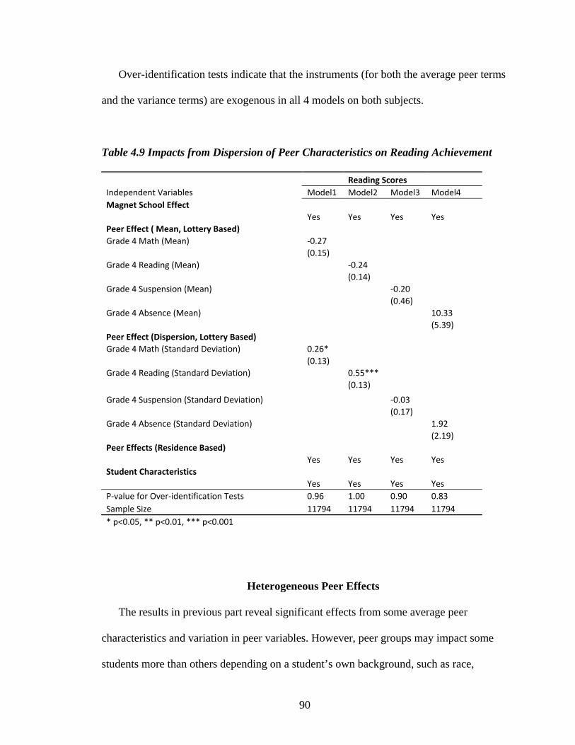
90

Over-identification tests indicate that the instruments (for both the average peer terms

and the variance terms) are exogenous in all 4 models on both subjects.

Table 4.9 Impacts from Dispersion of Peer Characteristics on Reading Achievement

Reading Scores



Yes Yes Yes Yes


Grade 4 Math (Mean) ‐0.27

(0.15)

Grade 4 Reading (Mean) ‐0.24

(0.14)


(0.46)


(5.39)


Grade 4 Math (Standard Deviation) 0.26*

(0.13)

Grade 4 Reading (Standard Deviation) 0.55***

(0.13)

Grade 4 Suspension (Standard Deviation) ‐0.03

(0.17)


(2.19)


Yes Yes Yes Yes


Yes Yes Yes Yes


Sample Size 11794 11794 11794 11794

* p<0.05, ** p<0.01, *** p<0.001

Heterogeneous Peer Effects

The results in previous part reveal significant effects from some average peer

characteristics and variation in peer variables. However, peer groups may impact some

students more than others depending on a student’s own background, such as race,

91

gender, or academic ability. This section answers the third research question “to whom

do peer effects matter more”. To examine this possibility, I interact all peer group

variables with individual characteristics, including black, Low SES, female, and

indicators of student academic ability.29 The student academic ability indicators are

measured by student initial position in each cohort lottery participants’ achievement

distribution in 4th grade: if a student’s prior math score is in the bottom quartile (1st) of

math score distribution among lottery participants, this student is coded as a low math

achiever; if a student’s prior math score is in the top quartile (4th) of the distribution,

he/she is coded as a high math achiever. The same procedure is also applied to reading

achievement. Therefore, there are four academic ability indicators for one student: high

math achiever, low math achiever, high reading achiever, and low reading achiever. The

four indicators along with three demographic variables are interacted with all 10 peer

variables to investigate if there are heterogeneous peer effects.

As shown in previous part, not every peer characteristic has shown a significant

impact on student outcomes. Therefore, although all 10 specifications of peer

characteristics are examined in the investigation of heterogeneous peer effects, I’m only

going to report the results from two widely expressed contextual peer characteristics

(percent black students and percent low SES students30 ) and from the other four peer

29 Because there are very few Hispanic, Ell, and Special Education students among the lottery participants (especially for the academic magnet program), I only choose three student demographic variables (black, female, and SES) to interact with the peer characteristics. Also, due to the fact that most lottery participants never received suspension and have very low absence rate, more than 80% students will receive the value of 1 as low disciplinary incidences based on the quartiles, and very few will be coded as high misbehaving group. Therefore, I only create the academic ability indicators, which are also used in Haneshek et al (2002) and Kang (2007) in examining heterogeneous peer effects. 30 Another widely expressed peer variable is peer gender composition (percent female students), I did not include in the tables here because most models (at both levels) find no significant effect from this variable.

92

outcome variables (peer math and reading achievement, peer disciplinary incidence, and

peer absence rate).

Math Achievement

The regression model examining the heterogeneous peer effect is expressed in

equation (3.17) of Chapter III, in which the interaction of the peer variables with

individual characteristics is added into the model. The two regressors of interest then

include the average peer characteristics and the interaction term. As usual, since the

estimates of magnet school treatment effect, residential choice effect, and individual

characteristics do not change much from previous average peer effect models, Table 4.10

omits the coefficients on these variables.

Each column in Table 4.10 represents an individual background variable; each

horizontal panel represents a peer variable. The coefficients on the average peer term are

reported in each row of the mean effect; the coefficients on the interaction terms are

reported in each row of the heterogeneous effect. However, note that the coefficients on

the average peer term in Table 4.10 can not be interpreted as the overall estimates of

average peer effects on all students; instead, they should be explained as the average peer

effects on students of the group not indicated at the top of each column. The coefficients

on the heterogeneous terms stand for the peer effect differences between the two groups.

The estimated peer effects on the specific student group in each column are obtained as

the linear combination of the coefficient on the average term and the coefficient on the

interaction term31.

31 The combination test results will be reported in Appendix E.

93

Table 4.10 Heterogeneous School Level Peer Effects on Math Achievement

Math Scores

Model1 Model2 Model3 Model4 Model5 Model6 Model7

Black LSES Female

Low Reading Achiever

High Reading Achiever

Low Math Achiever

High Math Achiever

Peer Effects (Lottery Based)

Proportion of Black Students Mean Effect ‐0.43** ‐0.48** ‐0.66*** ‐0.47** ‐0.46** ‐0.39** ‐0.45**

(0.18) (0.16) (0.16) (0.15) (0.15) (0.15) (0.15)

Heterogeneous Effect ‐0.11 ‐0.04 0.32*** ‐0.09** ‐0.16** ‐0.22*** ‐0.18***

(0.09) (0.10) (0.07) (0.03) (0.05) (0.03) (0.05)

Proportion of Low SES Students

Mean Effect ‐0.33 ‐0.36* ‐0.48** ‐0.30 ‐0.30 ‐0.22 ‐0.28

(0.18) (0.18) (0.18) (0.18) (0.18) (0.18) (0.18)

Heterogeneous Effect ‐0.00 0.14 0.22** ‐0.11** ‐0.18** ‐0.27*** ‐0.20***

(0.10) (0.13) (0.08) (0.04) (0.06) (0.04) (0.05)

Peer Prior Math Achievement

Mean Effect 0.04 0.04 0.14 0.05 0.06 0.07 0.03

(0.17) (0.17) (0.17) (0.17) (0.17) (0.17) (0.17)

Heterogeneous Effect 0.06 ‐0.01 ‐0.08* ‐0.09* ‐0.09** ‐0.05 ‐0.13***

(0.04) (0.05) (0.03) (0.04) (0.03) (0.04) (0.03)

Peer Prior Reading Achievement

Mean Effect 0.10 0.10 0.18 0.12 0.12 0.13 0.10

(0.15) (0.15) (0.15) (0.15) (0.15) (0.15) (0.15)

Heterogeneous Effect 0.04 ‐0.03 ‐0.07* ‐0.08* ‐0.08** ‐0.06 ‐0.12***

(0.04) (0.05) (0.03) (0.03) (0.03) (0.03) (0.03)

Peer Prior Disciplinary Records

Mean Effect ‐0.17 ‐0.14 ‐0.23 ‐0.03 ‐0.04 0.13 0.09

(0.23) (0.21) (0.23) (0.20) (0.20) (0.20) (0.21)

Heterogeneous Effect 0.18 0.17 0.25 ‐0.20 ‐0.28 ‐0.58*** ‐0.71***

(0.20) (0.23) (0.19) (0.12) (0.18) (0.12) (0.16)

Peer Prior Attendance Records

Mean Effect 0.97 0.89 0.31 2.48 2.08 3.01 2.35

(4.86) (4.69) (5.08) (4.69) (4.69) (4.68) (4.68)

Heterogeneous Effect 4.86 5.48 2.60 ‐1.83*** ‐2.50*** ‐3.45*** ‐3.51***

(4.05) (4.55) (3.44) (0.51) (0.63) (0.50) (0.61)

* p<0.05, ** p<0.01, *** p<0.001

94

The first peer variable reported in the table is percent Black students. The results from

model 1 and model 2 suggest that although individual math score appears to be lower in a

school with high percentage of black students, there is little evidence showing that Blacks

or low income students are more severely impacted by school racial composition. This is

different from previous findings of Hanueshek et al (2002) and Hoxby (2000), who both

find stronger intra-racial group peer effects for Black students. However, although the

heterogeneous effect is not statistically significant for black students, the linear

combination test in Model 1 shows a coefficient of 0.55 (P<0.01) on black students,

which is still bigger than the coefficient on non-black students (0.43). Female students,

however, are much less strongly impacted than males by school percent black students.

For instance, switching from a school with 25% black students to another school with

75% black students is likely to lower the math scores for boys by 0.33 points of

standardized scores; but for girls, the achievement reduction is only 0.17, about half the

size of the impact on boys. Interestingly, models 4 to 7 suggest that the estimated effect

of school percent black students appears to be stronger on both low achievers and high

achievers. Recall that the estimate of percent Black student effect on all lottery

participants is 0.49 in the average peer effect model (model 1 in Table 4.5). The

heterogeneous peer effect models find the percent black student coefficients (linear

combination coefficients) are higher on students at both the bottom and the top quartiles

of achievement distribution: 0.56 for low reading achievers, 0.61 for high reading

achiever, 0.61 for low math achievers, and 0.63 for high math achievers. All 4

coefficients are statistically significant at 1% level.

95

The second peer variable examined here is percent low SES students. Although there

is no significant effect of percent low SES students on the whole lottery participant

sample (as shown in Model 2 of Table 4.5), the heterogeneous models find that school

percent low income students does have significant impact on some student groups. First,

the estimate of percent low SES student effect is significant (P<0.05) on students from

more affluent families (students who are not eligible for free and reduced lunch

programs). Second, boys are much more likely to score lower if they are in a school with

high percentage of low SES peers. The coefficient is quite large (-0.48), which suggests

that a 50 percentage point change in school low SES population will affect the average

math performance by 0.24 points of standardized score for boys; in contrast, the

estimated effect is much less sizeable and not significant for girls. Third, students in both

the bottom and top quartiles of achievement distribution seem to be more impacted by the

changes in school low SES population. For instance, the linear combination coefficients

for both low math achievers and high math achievers are -0.49 and are statistically

significant at 1 percent level.

The next two peer variables are the lagged measures of peer math and reading

achievement. The results from all models on these two variables are very similar. First,

school average peer achievement (in both math and reading) does not have significant

influence on individual math scores; and there is no heterogeneous effect on black

students or low SES students. Second, although girls and students in both the bottom and

top achievement quartiles appear to be more negatively impacted by average peer

achievement, the linear combination tests do no reveal significant effects on these groups

of lottery participants.

96

The fifth peer variable is peer average disciplinary infraction, which has shown no

significant impact on student math scores from the average peer effect model (Model 9 in

Table 4.5). Heterogeneous effect of this peer discipline variable is only found in two

models: both high math achievers and low math achievers are much more strongly

influenced by peer disciplinary behaviors than other students. The linear combination

coefficient for students in the top quartile of math achievement distribution is -0.62

(P<0.01), which suggests that if half of the school peers received 1 more suspension in 4th

grade, high math performing lottery participants are likely to score lower by 0.3 points of

standardized score in math.

The last peer variable is average school peer absence rate, which represents peer

attendance behavior. There is no significant influence from the average attendance

behavior of peers on student math achievement in middle school. No heterogeneous

effects are found from the interactions of this peer variable with the three demographic

characteristics. Although the estimates of peer attendance behavior appear to be different

on students in both the bottom and top quartile of achievement distribution, the linear

combination tests do not find the coefficients significant.

Reading Achievement

The estimates of heterogeneous peer effect models are presented in Table 4.11. The

first peer variable is percent Black students. Recall that the average peer effect model

(model 1 in Table 4.7) does not reveal significant peer effect from this variable on student

reading achievement. Table 4.11, however, finds some significant heterogeneous effects.

First, boys tend to have worse math performance if they attend a school with high

97

proportion of black peers, while the negative impact is much smaller and insignificant

(the linear combination coefficient) on girls. Second, the estimates of heterogeneous peer

racial composition effects are significant on both low and high reading achievers.

Especially for the students in the top quartile of reading score distribution, the linear

combination coefficient is -0.54 (P<0.001), which is more than 5 times of the coefficient

for other students whose prior reading scores are lower. Low math performing students

also appear to be more negatively impacted by average school percent black students than

other students, but the linear combination coefficient is not significant.

The second peer variable is percent low SES students. Significant heterogeneous

effects are found for female students, students in both the bottom and top quartiles of

reading achievement distribution, and low math achievers. However, the estimated effect

of average school percent low SES students is only significant on the reading

achievement of high reading achievers --- the linear combination coefficient is -0.34

(P<0.05), suggesting that increasing the school low SES population from 25% to 75%

tends to reduce the average reading score by 0.17 points of standardized scores for

students with high reading skills.

The third peer variable is peer math achievement. Both high and low reading

achievers are more negatively impacted by average peer math achievement than other

students. The linear combination coefficients on both groups are -0.38 and significant at

5% statistical level, suggesting that lottery participants at both the top and bottom math

achievement distribution are likely to perform worse in reading if their school peers have

better prior math achievement. There are no significant findings for other groups of

students.

98

Table 4.11 Heterogeneous School Level Peer Effects on Reading Achievement

Reading Scores


Black LSES Female



Low Math Achiever

High Math Achiever


Proportion of Black Students Mean Effect ‐0.15 ‐0.21 ‐0.30* ‐0.16 ‐0.10 ‐0.17 ‐0.19

(0.16) (0.15) (0.15) (0.14) (0.14) (0.14) (0.14)

Heterogeneous Effect ‐0.09 0.06 0.19** ‐0.18*** ‐0.43*** ‐0.07* ‐0.05

(0.09) (0.09) (0.06) (0.03) (0.04) (0.03) (0.04)

Proportion of Low SES Students

Mean Effect 0.06 0.05 ‐0.05 0.11 0.14 0.09 0.06

(0.17) (0.17) (0.17) (0.17) (0.17) (0.17) (0.17)

Heterogeneous Effect ‐0.04 0.01 0.15* ‐0.23*** ‐0.48*** ‐0.10** ‐0.03

(0.09) (0.12) (0.08) (0.04) (0.05) (0.04) (0.05)


Mean Effect ‐0.30 ‐0.30 ‐0.28 ‐0.27 ‐0.27 ‐0.31 ‐0.30

(0.16) (0.16) (0.16) (0.16) (0.16) (0.16) (0.16)

Heterogeneous Effect 0.06 ‐0.01 ‐0.01 ‐0.15*** ‐0.13*** 0.03 ‐0.05

(0.04) (0.05) (0.03) (0.04) (0.03) (0.03) (0.03)


Mean Effect ‐0.30* ‐0.30* ‐0.29* ‐0.26 ‐0.27 ‐0.31* ‐0.29*

(0.14) (0.14) (0.14) (0.14) (0.14) (0.14) (0.14)

Heterogeneous Effect 0.05 ‐0.00 ‐0.00 ‐0.14*** ‐0.11*** 0.03 ‐0.04

(0.03) (0.05) (0.03) (0.03) (0.03) (0.03) (0.03)


Mean Effect ‐0.25 ‐0.36 ‐0.11 ‐0.09 ‐0.13 ‐0.24 ‐0.18

(0.21) (0.20) (0.22) (0.19) (0.19) (0.19) (0.19)

Heterogeneous Effect ‐0.04 0.24 ‐0.26 ‐0.56*** ‐0.82*** ‐0.09 ‐0.37*

(0.19) (0.21) (0.18) (0.11) (0.16) (0.11) (0.15)


Mean Effect 12.64** 13.47** 14.02** 13.10** 12.28** 12.51** 12.28**

(4.62) (4.47) (4.83) (4.46) (4.45) (4.47) (4.47)

Heterogeneous Effect ‐1.96 ‐5.74 ‐2.66 ‐3.65*** ‐4.93*** ‐0.97* ‐0.69

(3.83) (4.30) (3.26) (0.48) (0.59) (0.47) (0.58)

* p<0.05, ** p<0.01, *** p<0.001

99

Average peer prior reading achievement has been found negatively associated with

student reading scores in middle school. The estimates of heterogeneous models suggest

that both high and low reading achievers are 50% more negatively impacted by average

school peer prior reading achievement --- the linear combination coefficients are about

0.40 and significant at 1% level.

Average school peer disciplinary infractions (the fifth peer variables), significantly

reduces the reading test scores of both high and low reading achievers. The

heterogeneous effect is particularly large for students who are in the top quartile of

reading achievement distribution. Linear combination test of Model 5 finds that when

average school peer disciplinary infractions increase by 0.5, reading scores of high

reading performing students falls by almost 0.47 in standardized scores (P<0.001) --- the

estimate if very substantial.

The last peer variable is peer attendance behavior, measured by average peer absence

rate. Overall, there is a positive correlation between average peer absence rate and

student reading achievement. However, three subgroups, the high and low reading

achievers, and low math achievers, appear to be less strongly impacted by peer

attendance behavior than other students. Moreover, the linear combination tests suggest

no significant effects of average peer absence rate on the reading scores of low income

students or students with high reading abilities.

The heterogeneous peer effect models on both math and reading achievements reveal

that peer influences do affect students differently depending on their backgrounds.

Overall, the academic outcomes (in both math and reading) of female students are less

impacted by school peer compositions. Both strong and weak ability students (measured

100

by both math and reading skills) seem to be more strongly impacted by school racial and

SES composition, as well as peer disciplinary infractions; and interestingly, both groups

of students seem to be more negatively impacted by average school peer academic

achievement.

Recall that the regression sample in this study is limited to lottery participants and the

identification of peer effects relies on the differences between lottery losers in

neighborhood schools and lottery winners in magnet programs. Overall, lottery

participants attending neighborhood schools are superior (in terms of social economic

status, prior achievement, and prior disciplinary records etc.) than other students in the

same school, and are more likely to be grouped with other advantaged peers for classes.

Especially for high performing lottery participants, because they are really advanced

compared to other students in their neighborhood school, they may be placed with the

best teacher, receive special instructions and more attention. This may less likely happen

to high performing lottery participants in magnet schools because the overall peer quality

is high. Similarly, even a student is at the bottom quartile of the prior achievement

distribution among the lottery participants; he/she may still be a high performer in his

neighborhood school and be assigned to classes with high quality peers and good

teachers; while this again may not be true for the low performing lottery participants

attending magnet programs. These are the possibilities that cause the large negative effect

of peer achievement on students at both the top and bottom quartiles of prior achievement

distribution. Given that students are often tracked within schools, high ability students are

likely to be grouped with more advantaged students (e.g., fewer black students or low

101

SES students, and fewer students with behavioral problems), the conclusions from the

classroom level may be different, which will be examined in next chapter.

Robustness Checks

Previous sections have shown that some of the estimated peer effects are quite large,

which raises the question whether the estimates capture something other than the effect of

peers. In this section, I am going to check the robustness of the peer effect estimates. In

specific, there are three major problems as discussed in Chapter III. First, whether the

estimated peer effects are confounded with some unobserved heterogeneity in treatment

responses? Second, whether the estimates of peer effects capture some other unobserved

school factors, especially teacher qualities? Third, whether the estimated peer effects are

biased by sample attrition?

This section will address the above three problems in order. Although I did the

robustness checks for all models related to the three research questions, in order to save

some space, the following discussion will only focus on the average peer effect models

on math achievement32.

Heterogeneity in Treatment Response

Recall that in the average peer effect model (equation 3.11) the causal effect of peer

group is identified from the interaction between the lottery based peer term )ˆ( NM PP

and the treatment indicator id . Therefore, the estimate of peer group effect could be

confounded with unobserved heterogeneity in the treatment response ( i id ). It is hard to

32 The conclusions from other models are similar to the average peer effect model on math achievement; and the results are available upon request.

102

directly test this hypothesis. However, controlling for the observable heterogeneity in

treatment response can help to indirectly check whether the estimated peer effects are

proxies for the treatment response heterogeneity. In specific, we are going to control for

the interactions of the treatment indicators33 ( id ) with all individual characteristics in the

model, including prior achievement and behavioral outcomes. If controlling for all these

observable treatment response heterogeneity in the regression leads to a diminished

estimate of peer effect, then it indirectly proves that the estimated peer effect is in fact

confounded with the way different individual respond to treatment.

Table 4.12 presents the estimates of average school peer effect models on math

achievement, with the observed heterogeneity in treatment response controlled in the

regression. As shown in the table, including the interaction of treatment indicator with

individual variables in the model does not produce the expected changes in most of the

estimates of peer effects, especially not for the widely expressed peer characteristics,

such as peer race and SES composition, and peer academic achievement.

Some of the point estimates of peer effects become even larger than before (results in

Table 4.5), e.g., percent black students and percent low SES students. Especially, the

estimated effect of percent low SES students turns bigger and significant while

controlling for the heterogeneous treatment response term. The estimates of peer

academic ability measures (models 7and 8), and peer attendance behavior are also larger,

but they are still insignificant.

The point estimates of variables like percent female students, percent special

education students, and prior student discipline infractions, are a little smaller, but they

33 There are two treatment indicators, one for the academic magnet, and the other for the non-academic composite.

103

still remain significant. Including treatment response heterogeneity only overturns the

significant impact from one variable --- percent ELL students. The point estimate of

percent ELL students is about 40% smaller than the estimate from the original model

(model 6 in Table 4.5), and is not statistically significant.

Table 4.12: Average School Peer Effects on Math Achievement (Treatment Response Heterogeneity) Math Scores

Independent Variables Model1 Model2 Model3 Model4 Model5 Model6 Model7 Model8 Model9 Model10


Academic Treatment indicators are interacted with individual characteristics

Non‐Academic Composite Treatment indicators are interacted with individual characteristics

Peer Effect (Lottery Based) Black (proportion) ‐0.59***

(0.18)

Low SES (proportion) ‐0.41*

(0.18)

Female (proportion) ‐1.15*

(0.54)

Hispanic (proportion) ‐0.11

(0.63)

Special ED (proportion) 2.33*

(0.98)

ELL (proportion) 1.40

(1.22)

Grade 4 Math (Mean) 0.22

(0.15)

Grade 4 Reading (Mean) 0.20

(0.14)


(0.20)


(4.58)


Yes Yes Yes Yes Yes Yes Yes Yes Yes Yes



Sample Size 11780 11780 11780 11780 11780 11780 11778 11778 11778 11778

* p<0.05, ** p<0.01, *** p<0.001

104

Overall, the results from Table 4.13 do not support that the estimates of average

school peer effects are confounded with unobservable heterogeneity in treatment

response.

Unobserved School Factors

The second problem is whether the estimates of peer effects pick up some other

unobserved school characteristics, especially teacher qualities. A lot of research (e.g,

Ingersoll 1999, 2004; Peske & Haycock, 2006) has shown that low quality teachers are

more likely to be assigned to schools with high percent poor and minority students. In our

sample, if the neighborhood schools that lottery losers must attend (those schools usually

have higher percentage of black and low income students) tend to have less effective

teachers, then the estimates of peer effects may just be proxies for the school teacher

qualities.

To examine this possibility, I re-estimate the average peer effect models with teacher

fixed effects included in the regression. Introducing teacher fixed effect into the model

greatly reduces the variation in the data to estimate peer effects because the between-

teacher differences in peer characteristics are absorbed by the estimates of teacher effect.

Fortunately, we have 5 cohorts of students in the sample, which ensures a great within-

teacher variation in peer characteristics. Also, the district was undergoing a school

reassignment during the investigation years34, which also contributes to a great variation

in peer characteristics over the course of a teacher’s career.

34 The district moved from a court-ordered desegregation plan to a neighborhood-based school system during these years.

105

Table 4.13 presents the results from the teacher fixed effect models. Overall, the

estimates of peer effects have larger standard errors, which are expected given that

estimating teacher fixed effects requires a large amount of data. However, the new

models do not find any evidence that the estimated peer effects in the original models are

picking up the effects from school teachers. Instead, while teacher fixed effect is

controlled in the regression, some estimates of peer effects are even larger than earlier,

such as percent black students, percent special education peers and percent ELL students.

Table 4.13: Average School Peer Effects on Math Achievement (Teacher Fixed Effect)

Math Scores

Independent Variables Model1 Model2 Model3 Model4 Model5 Model6 Model7 Model8 Model9 Model10 Magnet School Effect Academic Treatment indicators are interacted with individual characteristics

Non‐Academic Composite Treatment indicators are interacted with individual characteristics


Black (proportion) ‐1.47* (0.63) Low SES (proportion) ‐0.16

(0.69)

Female (proportion) ‐1.44 (1.11)

Hispanic (proportion) 4.38*

(2.13)

Special ED (proportion) 5.49**

(2.17)

ELL (proportion) 7.22*

(3.52) Grade 4 Math (Mean) ‐0.34

(0.74) Grade 4 Reading (Mean) ‐0.34

(0.74)

Grade 4 Suspension (Mean) 0.03

(0.51)


(11.74) Peer Effects (Residence Based)


Student Characteristics Yes Yes Yes Yes Yes Yes Yes Yes Yes Yes

Sample Size 11764 11764 11764 11764 11764 11764 11762 11762 11762 11762

* p<0.05, ** p<0.01, *** p<0.001

106

In addition, I also implemented a set of school fixed effect models to check if the

estimated peer effects are confounded with some unobserved time-invariant school

factors, such as school policy and principal leadership. The school fixed effect model

results are very similar to the results from the teacher fixed effect models, and do not

support that the large estimates of peer effects are proxies for unobserved school factors.

Attrition Problems

All studies exploiting randomized experiment face a common problem --- attrition. In

our data, there are two types of attrition: (1) students do not continue to enroll in the

district schools in a year subsequent to the lottery --- they may switch to a private school,

or move to another district; (2) students do not have spring test scores. Not all of the

students in the second group are attritors for that they may still stay in the system --- there

are other reasons that no test scores may be reported. However, since a student without

test scores could not contribute to the estimation of peer effects, they pose the same

problem as the attritors.

If attrition from the lottery winners is the same as from the lottery losers, it will not

impact the difference in outcomes between these two groups and will not bias the

estimates of treatment effect and peer effect. Unfortunately, as shown in table 4.14, the

attrition rate of lottery winners is quite different from the rate of the lottery losers. The

discrepancy is particularly pronounced for lottery participants in the academic magnet

program --- losers are 50 percent more likely to leave the district than winners between

4th and 5th grade. The attrition rate of lottery losers continues to be larger than lottery

winners in later grades. For non-academic composite lottery participants, although the

107

attrition gap is smaller, lottery losers still have an attrition rate 40 percent higher than

lottery winners in the year subsequent to the lottery.

Table 4.14 Attrition Rates, by Lottery Outcomes1,2

Lotteries

Academic Non‐academic Composite

Winners Losers Winners Losers

Leave the system after grade

4 11.50% 17.45% 7.45% 10.58%

5 6.05% 12.01% 9.85% 6.57%

6 7.79% 9.94% 9.18% 6.23%

7 4.61% 8.20% 7.97% 6.02%

No spring Math scores in grade

5 4.00% 6.16% 6.60% 3.14%

6 1.73% 2.46% 3.46% 2.37%

7 1.61% 2.50% 2.24% 1.51%

8 1.08% 1.79% 2.13% 2.49%

1.Counts only students who were in the system as 4th grade students when the lotteries

were conducted and do not miss 4th grade math scores.

2. A student is defined as a lottery winner if he/she won the lottery outright on the lottery day

or received the delayed offer in 5th grade.

The lower part of Table 4.14 shows the percentage of students missing math scores in

the spring35. There is less significant difference between winners and losers who do not

have spring test scores. In 5th grade, academic magnet lottery losers are more likely to

miss math scores than lottery winners, and the pattern is opposite for the non academic

composite lottery participants. The between group gap is even smaller in later grades.

35 Students who miss spring test scores are different from the first type of attritor (those who left the district before a new school year started as indicated in the upper part of the table). They have records in the district attendance file and student file, but do not have the record of test scores in the state standardized tests. Although there are many reasons that test scores are not reported, many students may have left the system during the school year. For example, there are 337 academic magnet lottery participants who never enrolled in the system as 5th graders (they are considered as the first type of attritors); there are 100 participants who enrolled in district schools but were not present for testing (considered as students with missing scores). Among these 100 students, the majority of them had probably left the system prior to the test date, as 65% of them were never enrolled in 6th grade.

108

Therefore, I’ll only focus on the first type of attritors (those who do not return to the

system in the fall) in the following analysis.

Apparently, attrition is not random among lottery winners and lottery losers. Lottery

outcomes do affect the decision whether to stay or leave the system. The problem is

whether the correlation between attrition and student outcomes is systematically different

between lottery winners and lottery losers. For example, if the lottery losers who left the

system have families that are more concerned than the average about the quality of their

children’s schools (especially, more concerned about the peers in the school), attrition

may introduce systematic differences in outcomes between treatment group and control

group, and then bias the estimates of treatment effect and peer effect.

In this study, all regression models control for a large set of observed individual

characteristics, including prior achievement and behavioral records, which greatly

reduces attrition-induced bias36 . However, if attrition is correlated with some

unobservable variables, the differences between winners and losers may not be a simple

linear function of the observed student characteristics, then even these controls are not

enough to offset the bias caused by attrition. For example, if high achieving lottery losers

are more likely to leave the system when they have to return to a neighborhood school

that has a high percentage of disadvantaged peers, then attrition difference may bias the

estimate of peer effect upwards by removing high achievers from schools that have a

large population of minority and poor students.

36 To the extent that attrition-related outcome differences are a linear function of student demographic characteristics and 4th grade test scores and behavioral records, including these individual variables restore the balance between treatment and control groups.

109

To examine the attrition problem further, I estimate a model of attrition between

fourth and fifth grades among the academic magnet participants.37 The dependent

variable is a dichotomous variable indicating attrition: 1 if the student left the system in

5th grade; 0 otherwise. The independent variables are mostly limited to the regressors

already included in the achievement models, including lottery outcome indicator38 and

individual characteristics. If the results do not find a significant correlation between the

attrition and the observable characteristics that predict achievement, it is less plausible

that other unobservables with comparable predictive power could drive the decision of

attrition. In addition, four variables as functions of peer characteristics are also included

in the model to explore the possibility whether there is selective attrition among high

achieving students when they have had to attend a school with disproportional minority

and low income students. The four variables include: the school peer characteristics

(percent black and percent low income students) a student will face if he/she loses the

lottery NP( in the above notation); the interaction of lottery outcome indicator with NP ;

the interaction of individual prior math achievement with NP ; and a three way interaction

of individual prior math scores, lottery outcome indicator, and NP . Since the

neighborhood school peer characteristics should not affect a student’s attrition decision if

he won the lottery, one would expect the estimate on the second term (the interaction of

winning with NP ) to offset the effect of the stand-alone NP . Moreover, if the previously

described scenario is true, the coefficient on the interaction of prior math achievement

with NP should be positive, while the coefficient on the three way interaction are

37 The discrepancy in attrition rate is more pronounced in the year subsequent to the lottery between lottery winners and lottery losers in the academic magnet lottery. 38 Given that students have to make the private school enrollment decision in the spring, while the delayed win notice usually comes at the beginning of the fall semester, I only use the outright win indicator.

110

expected to be negative. Only two models are estimated--- one with the peer variable of

percent black and the other with percent low SES students.39

Table 4.15 presents the results from the two attrition models. Given the numerous

interactions included in the model, all coefficients have large standard errors and are very

imprecise. While the point estimate of percent school black students is positive as

expected, the estimate of percent low SES students is negative; the coefficient on winning

the lottery is negative which offsets the impact from the stand-alone peer characteristics.

However, the coefficients on the interaction of peer characteristics with prior math

achievement are negative, which works opposite to the hypothesis that high achieving

students are more likely to leave the system if they had to return to a neighborhood

school with more disadvantaged students; the coefficients on the three way interaction are

also unexpectedly positive.

39 The reasons to choose these two peer variables include: (1) these are two school characteristics that are usually released to the public, such as posted on the district website. It is easier for parents to check school racial composition and SES composition than to check other school peer characteristics, such as average prior achievement, disciplinary records, or special education students. Therefore, they are likely to be the major factors influencing parents’ decision on school enrollment. (2) these two peer variables are found significantly influencing student math achievement as shown in Table 4.5. Although the overall coefficient on average percent low SES peers is not significant in Table 4.5, the heterogeneous effect table (Table 4.10) shows that many groups of students are negatively impact by school low income population. (3) these are commonly expressed peer characteristics examined in the literature.

111

Table 4.15 Effects of Lottery Outcomes and Peer Characteristics on Attrition Attrition

Model 1 Model 2

Independent Variables

Outright Winner ‐0.43 ‐0.3 (0.48) (0.47)

Percent Black 0.32 (0.48)

Percent Black * Winner ‐0.38 (0.91)

Percent Black * 4th grade math ‐0.22 (0.35) Percent Black * 4th grade math*winner 0.02 (0.62) Percent low SES ‐0.47 (0.51)

Percent low SES * Winner ‐0.74 (0.96)

Percent LOW SES * 4th grade math ‐0.16

(0.37)

Percent LOW SES * 4th grade math*winner 0.49 (0.66)

4th grade math scores 0.06 0.02

(0.17) (0.17)

4th grade math scores *winner 0.12 ‐0.07

(0.29) (0.29)

4th grade reading scores 0.05 0.04

(0.06) (0.07)

4th grade reading scores *winner 0.14 0.15 (0.11) (0.11)

Black ‐0.49** ‐0.44** (0.13) (0.13)

Black*winner 0.13 0.08

(0.24) (0.23)

Low SES ‐0.09 ‐0.02

(0.13) (0.13)

Low SES*winner 0.01 0.03 (0.26) (0.26)

Special Ed ‐0.57 ‐0.62 (0.53) (0.54)

Special Ed*winner 0.52 0.58

(0.79) (0.79)

ESL ‐0.33 ‐0.31 (0.51) (0.51)

ESL*winner 0.63 0.60

(0.78) (0.78)

Female 0.03 0.02

(0.08) (0.08)

Female*winner 0.10 0.07 (0.15) (0.15)

No. of Observation 2275 2275

* p<0.05, ** p<0.01, *** p<0.001

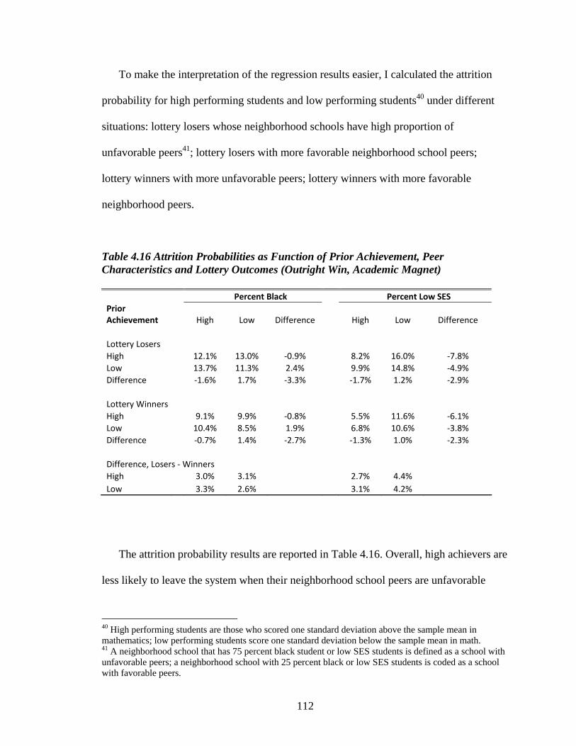
112

To make the interpretation of the regression results easier, I calculated the attrition

probability for high performing students and low performing students40 under different

situations: lottery losers whose neighborhood schools have high proportion of

unfavorable peers41; lottery losers with more favorable neighborhood school peers;

lottery winners with more unfavorable peers; lottery winners with more favorable

neighborhood peers.

Table 4.16 Attrition Probabilities as Function of Prior Achievement, Peer Characteristics and Lottery Outcomes (Outright Win, Academic Magnet)

Percent Black Percent Low SES

Prior Achievement High Low Difference High Low Difference

Lottery Losers

High 12.1% 13.0% ‐0.9% 8.2% 16.0% ‐7.8%

Low 13.7% 11.3% 2.4% 9.9% 14.8% ‐4.9%

Difference ‐1.6% 1.7% ‐3.3% ‐1.7% 1.2% ‐2.9%

Lottery Winners

High 9.1% 9.9% ‐0.8% 5.5% 11.6% ‐6.1%

Low 10.4% 8.5% 1.9% 6.8% 10.6% ‐3.8%

Difference ‐0.7% 1.4% ‐2.7% ‐1.3% 1.0% ‐2.3%

Difference, Losers ‐ Winners

High 3.0% 3.1% 2.7% 4.4%

Low 3.3% 2.6% 3.1% 4.2%

The attrition probability results are reported in Table 4.16. Overall, high achievers are

less likely to leave the system when their neighborhood school peers are unfavorable

40 High performing students are those who scored one standard deviation above the sample mean in mathematics; low performing students score one standard deviation below the sample mean in math. 41 A neighborhood school that has 75 percent black student or low SES students is defined as a school with unfavorable peers; a neighborhood school with 25 percent black or low SES students is coded as a school with favorable peers.

113

(column 1 and column 4); and low achievers are less likely to exit when the situation is

reversed --- with more favorable neighborhood school peers (column 2 and column 5).

This pattern holds for both lottery winners and lottery losers in both peer characteristics;

and it works against finding large peer effects.

Under any scenario, lottery losers are more likely to leave the system. However, a

more important problem is whether the attrition rate gap between high performing lottery

losers and lottery winners is different from the gap between lottery losers and lottery

winners who are low performers. Overall, the loser-winner difference is modest as

reported in the bottom panel. When the neighborhood school peers are unfavorable, the

attrition gap is larger for low achievers than for high achievers; the reverse is true when

peers are favorable --- the loser-winner difference is bigger for high achievers than for

low achievers. These findings again, do not support the hypothesis that differential

attrition biases the estimates of peer effects upward by removing high performing lottery

losers from schools serving high proportion minority and poor students.42

The final step to assess the attrition impact is to re-estimate the achievement model

(with only two peer characteristics examined, percent Black and percent low SES

students) using a weight option. Each observation is weighted by the inverse of the

predicted probability that the student remains in the school system; therefore, the

weighted sample resembles what the sample would be if no student had left the system.

The stay-in-system probability (the inverse of the weight) equals 1 minus the attrition

42 However, one thing should be mentioned that the linear combinations of the coefficients reported in Table 4.17 have large standard errors and overlapping confidence intervals, so we can not reject the hypothesis that high performing students do not differ from low performing students in attrition rate, regardless of the peers and lottery outcomes.

114

probability, which is calculated from a more general attrition model than the one shown

in Table 4.15.43

The estimates of peer effects are quite similar to those in Model 1 and Model 2 of

Table 4.6. The coefficient on percent Black from the weighted model is -0.53 (P<0.001),

virtually identical to the coefficient (-0.49, P<0.001) in Table 4.6. The coefficient on

percent low SES students from the weighted model is -0.43 (P<0.05), which is even

larger than the one in original model (-0.33) and is weakly significant (at 5% level) in

statistical sense.

To conclude, although there is significant attrition from our data, with more lottery

losers leaving the system than lottery winners, there are no systematic differences

between the remaining (or attrited) lottery losers and lottery winners in the correlation

between all observed characteristics and achievement. Therefore, there is no evidence

that attrition has biased the estimates of magnet school treatment effects and the peer

group effects.

43 The attrition model is very similar to the one shown in Table 4.15, but includes lottery participants in both the academic magnet and the non-academic composite, and has separate equations for attrition after each grade. For instance, the attrition equation after grade 5 includes 5th grade test scores as additional controls; the one after grade 6 includes 6th grade achievement; the one after grade 7 includes 7th grade test scores.

115

CHAPTER V

PEER EFFECTS ON ACADEMIC ACHIEVEMENT ---RESULTS FROM CLASSROOM LEVEL ANALYSIS

This chapter explores how the classroom peer composition impacts student academic

achievement in math and reading. Last chapter finds significant peer effects from some

school peer characteristics, such as percent Black students, but no evidences that average

school peer academic abilities or peer disciplinary records influence student achievement

in middle school. Intuitively, it is expected that peer effects at the classroom level should

be stronger than the school level peer effects since classroom is the place where

instruction happens and peer interactions in academics mostly take place. In this chapter,

I am going to examine how classroom peers influence student achievement and whether

the magnitude of classroom peer effects is larger than that of school peer effects.

As discussed in Chapter III, identifying classroom peer effects poses more

econometrical challenges, including selection bias arising from the non-random

classroom placements and omitted variable bias which is likely to be stronger at the

classroom level. This section overcomes these methodological challenges by exploiting

the admission lotteries that randomly assign students to a magnet school or a

neighborhood school. In particular, each student in both the treatment group and the

control group is assigned a predicted value of counterfactual classroom peers, which is

close to the class peers that a student would encounter if he had been in the opposite

situation. The prediction of the counterfactual peer characteristics utilizes a rich set of

information including lottery outcomes, individual characteristics, prior outcomes, and 4th

116

grade schools. The exogenous estimates of the classroom peer effects on student

achievement can then be derived from the differences between the actual classroom peer

characteristics and the counterfactual classroom peer characteristics.

The descriptive statistics of classroom peer characteristics has already been reported

in Chapter III; therefore this chapter will skip the section of descriptive results. The first

three sections in this chapter are organized to answer the three research questions on: (1)

average classroom peer effects on student achievement; (2) the impact from dispersion of

classroom peer characteristics; (3) the heterogeneous classroom peer effects. The fourth

section checks the robustness of the estimates with a focus on whether the estimated

classroom peer effects are proxies for classroom instructors. The final section discusses

the differences between school level peer effects and classroom level peer effects.

Impacts from Average Classroom Peer Characteristics

The model used to estimate average classroom peer effect is equation 3.17. The major

regressor of interest is cijP , the actual classroom peer characteristics. To deal with he

endogeneity of the classroom peer variable, I constructed an instrumental variable

consisting of the enrollment probability and counterfactual class peer characteristics.

Other important variables included in the equation are the magnet school treatment

indicators, residence based school peer characteristics44, and individual characteristics

(including prior outcomes).

The majority of middle school students usually rotate through classrooms for

different subjects, so the achievement models in this chapter estimate subject-specific

44 The residence based school peer characteristics are included in the model in order to control for the correlation between family residence choice and achievement.

117

peer effects on student academic achievement. The peer variables used in the math

achievement model are the average peer characteristics of one’s math classes; the

variables used in the reading achievement model are the average peer values of the

reading/language classes.45,46

Math Achievement

Table 5.1 presents the estimates of classroom peer effects on math achievement. Only

coefficients on the lottery based classroom peer variables and the magnet school

treatment indicators are reported in the table.47 Model 1 and model 2 suggest that student

math achievement is negatively impacted by classroom percent Black students and

percent low income students. The estimates of peer effects from these two classroom peer

variables are quite large: the average math score decreases by 0.33 points in standardized

score if the classroom black students increase from 25% to 75%; and a 50 percent point

change in classroom low income students is related to 0.4 point change in standardized

math scores. Moreover, the treatment effect of the academic magnet school turns to

negative (significant at 5% level) when classroom percent low income student is

controlled. This implies that a student would do even better in his neighborhood school if

he attends a class in the neighborhood school that has the same percent of low income

peers as his class in the academic magnet school.

45 If a student took multiple classes in one subject, the peer variable is an average value across all courses in this subject. 46 Schools have different titles for reading and language classes, for example, the same class may be titled Reading in some school, but as Language Arts (or English) in other schools. Therefore, we coded the class as reading class if the course id starts with ENG (the district course id for reading/language arts classes), but excludes some selective classes such as Creative Writing or Theater. 47 The coefficients on student characteristics are not included in the table because they are quite similar to previous results. The coefficients on majority of the residence based school peer characteristics are quite small and insignificant; and the conclusions on these estimates are similar to those from the school level models.

118

Table 5.1 Average Classroom Peer Effects on Math Achievement (Math Class)

Math Scores

Independent Variables Model1 Model2 Model3 Model4 Model5 Model6 Model7 Model8 Model9 Model10 Model11 Magnet School Effect

Academic 0.00 ‐0.09* 0.12** 0.09* 0.09* 0.21*** ‐0.09 ‐0.19** 0.08* 0.07 ‐0.08 (0.03) (0.05) (0.04) (0.04) (0.04) (0.06) (0.05) (0.05) (0.04) (0.05) (0.07) Non‐Academic Composite 0.11 0.02 0.13 0.11 0.09 0.18 0.06 0.00 0.11 0.06 0.02

(0.08) (0.09) (0.09) (0.09) (0.09) (0.09) (0.09) (0.09) (0.09) (0.10) (0.11)


Black (proportion) ‐0.66*** ‐0.08

(0.09) (0.43)


(0.10) (0.33)


(0.25) (0.26)

Hispanic (proportion) ‐0.88 ‐2.28*

(0.70) (1.07)

Special ED (proportion) ‐0.87* ‐0.43

(0.34) (0.52)

ELL (proportion) 2.82* 4.47

(1.29) (2.45)

Grade 4 Math (Mean) 0.32*** 0.03

(0.05) (0.22)

Grade 4 Reading (Mean) 0.40*** 0.15

(0.05) (0.14)

Grade 4 Suspension (Mean) ‐0.65*** 0.24

(0.20) (0.30)

Grade 4 Absence (Mean) ‐6.73 1.99

(4.05) (6.85)


Yes Yes Yes Yes Yes Yes Yes Yes Yes Yes Yes Student Characteristics Yes Yes Yes Yes Yes Yes Yes Yes Yes Yes Yes


Sample Size48 10224 10224 10224 10224 10224 10224 10224 10224 10224 10224 10224

* p<0.05, ** p<0.01, *** p<0.001

48 The sample size for classroom level analysis is smaller than that for school level analysis is due to two reasons: (1) Some lottery participants are not included in the course file so we are not able to construct classroom peer variables for them. (2) The academic magnet school did not report course information during school years 1999-2003. We are able to use homeroom number to calculate class peer variables for students in this school. However, due to the tracking policy in later grades, homeroom peer characteristics are quite different from the true class peer characteristics in grades 7 and 8. After consulting with the school former principle, we decided to include only 5th and 6th graders in school year 2000 to 2003 in the regression sample. Therefore, we exclude lottery participant observations from the following cohort: lottery year 1999 participants (7th graders in 2002 and 8th graders in 2003) and lottery year 2000 participants (8th graders in 2003).

119

The third significant finding is on classroom percent special education students

(Model 5), which is found significantly decreasing student math scores in middle school.

For instance, a 10 point percentage change in classroom percent special education

students is associated with a 0.09 point standardized score change in math achievement.

The estimated effect is quite large. Note that students eligible for special education

programs are often placed in the same class to meet their needs: in our data, the average

class percent special education peers is 0.33 for lottery participants who are also

identified as special education; and it is only 0.03 for non special education lottery

participants. The problem then is whether the negative impact of classroom percent

special education peers mainly works on those who are identified as special education

students. This will be addressed in the third section of heterogeneous peer effects. Also

note that the estimate of percent special education peers at the classroom level is opposite

to the estimate at school level which shows positive impact on student achievement. The

difference between the classroom estimate and school level estimate will also be

discussed later.

Model 6 in Table 5.1 finds that student math achievement tends to increase if there

are more ELL students in their class. The estimated effect is substantial: if the classroom

percent ELL students increases by 5% (one standard deviation of this peer variable in our

sample), the average math score improves by 0.14 standardized score. Interestingly, the

estimate of percent ELL students at the classroom level is very close to the estimate at the

school level, both indicating a positive correlation between student math scores and

percent ELL peers, at least in our sample.

120

The two peer academic ability variables, measured by average 4th grade math and

reading scores, have shown significant and positive impact on individual math

achievement in middle school. The sizes of the estimated effects from both peer academic

ability indicators are substantial. For example, a student’s math score in middle school

improves by 0.32 points in standardized scores if the average class prior math

achievement increases by 1 point (also in standardized scores); the estimated effect of

average class reading achievement is even larger. Also note that the treatment effect of

the academic magnet school is negative when the academic quality of class peers is

controlled. Model 8 finds a coefficient of -0.19 (P<0.01) on the academic magnet

treatment indicator, which suggests that lottery losers of the academic magnet school

would perform 0.19 standardized score higher in mathematics than the winners enrolling

in the academic program if the average class peer prior reading achievement in the

neighborhood school is the same as the academic magnet school. This implies that once

the classroom peer academic ability is controlled, students enrolled in the academic

magnet program are actually worse off in academics than their counterpart students in

neighborhood schools.

The result from Model 9 shows that average classroom peer disciplinary infractions

greatly decrease student math achievement in middle school. The coefficient on this

variable is -0.65 (P<0.001), implying that if half of the peers in the same class received

one more suspension in 4th grade, the average math score will decrease by 0.33

standardized score --- the effect is very large.

The classroom level analyses do not find significant impacts from percent Female

students, percent Hispanic students, and peer attendance behaviors. In column 11, all

121

specifications of peer characteristics are incorporated in one model. Due to the

collinearity of all these variables49, the estimated effects of most peer variables are no

longer significant. Only the variable percent Hispanic student shows weakly significant

and negative effect in the full variable model. Moreover, with all peer characteristics

included in one equation, neither of the two magnet programs is found influencing

student achievement --- the coefficient on the treatment indicator is negative for the

academic magnet. Again, the findings suggest that once we control for the class peer

composition, the magnet program is no more successful than the regular public schools in

this district, at least not in improving student math achievement.

Reading Achievement

Table 5.2 reports the regression results of classroom peer effects on student reading

achievement. Most estimates of peer effects on reading achievement are similar to the

estimates from the math achievement models. First, classroom race composition and SES

composition have strong and negative impact on student reading scores as shown in

model 1 and model 2. Second, peer academic abilities (model 7 and model 8), measured

by average peer math and reading scores in 4th grade, significantly improve individual

reading achievement in middle school. Third, average class peer disciplinary behavior

has shown strong and negative influence on student reading score. Interestingly, the point

estimate of the peer behavior effect on reading achievement (0.95) is almost 50% larger

than the estimated effect on math achievement (0.65): if every peer in the class received 1

49 Given the ability grouping policies in many schools, it is likely that the classroom peer characteristics are highly correlated.

122

more suspension in 4th grade, the average class reading score decreases almost 1 point in

standardized score. 50

Table 5.2 Average Classroom Peer Effects on Reading Achievement (Reading Class)

Reading Scores



Academic 0.02 ‐0.07 0.13*** 0.11** 0.11** 0.10 ‐0.04 ‐0.11* 0.06 0.12* ‐0.06

(0.03) (0.04) (0.04) (0.04) (0.04) (0.06) (0.06) (0.05) (0.03) (0.06) (0.09) Non‐Academic Composite 0.05 ‐0.02 0.07 0.06 0.06 0.06 0.01 ‐0.02 0.04 0.06 0.01

(0.08) (0.08) (0.08) (0.08) (0.08) (0.09) (0.08) (0.08) (0.08) (0.11) (0.12) Peer Effect (Lottery Based)

Black (proportion) ‐0.49*** ‐0.18

(0.10) (0.28)


(0.10) (0.27)


(0.25) (0.26)

Hispanic (proportion) ‐0.67 0.08 (0.85) (1.48) Special ED (proportion) ‐0.16 ‐0.11

(0.48) (0.67) ELL (proportion) ‐1.13 ‐1.85 (1.90) (3.10) Grade 4 Math (Mean) 0.23** ‐0.24 (0.07) ‐0.21

Grade 4 Reading (Mean) 0.30*** 0.22 (0.05) (0.20)

Grade 4 Suspension (Mean) ‐0.93*** ‐0.55*

(0.18) (0.25)

Grade 4 Absence (Mean) ‐0.54 0.90

(6.01) (8.77)



Student Characteristics Yes Yes Yes Yes Yes Yes Yes Yes Yes Yes Yes


Sample Size 10246 10246 10246 10246 10246 10246 10246 10246 10246 10246 10246

* p<0.05, ** p<0.01, *** p<0.001

50 The vast majority students in our sample took multiple reading/language classes, but only one (15% of the students took two) math class. The reading class peer characteristics assigned to one student is an averaged value across all the reading/language courses, so one point change in the average reading class peer disciplinary infraction usually means that the student has encountered more misbehaving peers in classes than one point change of average disciplinary infraction in math class. Therefore, it is not surprising the estimate of reading class peer behavior problem is larger.

123

Other peer variables, including percent special education students and percent ELL

classmates (they have shown significant impact on math achievement), are not found

significantly associated with student reading achievement. When all peer characteristics

are included in one model (Column 11), only the estimate of average peer disciplinary

infraction still remains strong and negative. Again, when the classroom peer composition

is controlled, neither of the magnet programs has shown any positive impact on student

reading achievement.

All models from both Table 5.1 and Table 5.2 are over-identified. The omnibus over-

identification tests suggest that the instruments (for both the treatment indicators and the

peer variables) in both math and reading achievement models are exogenous.


Ability tracking in schools has long been a controversial topic. Supporters of within

school tracking argue that putting similar students in classes can improve instructional

efficiency, while opponents argue that ability grouping would essentially harm low-

ability students by isolating them from peers with high ability and high motivations. In

this section, I am going to use the classroom data to examine how the heterogeneity of

classroom peer composition influences student academic achievement --- whether

students benefit from a more homogeneous class setting or they perform better in a class

with students at various levels in academic qualities.

Table 5.3 presents some descriptive statistics on the peer composition heterogeneity

variables, measured by the standard deviations in peer math and reading achievements,

peer disciplinary infractions, and peer absence rates. Overall, the classroom peer

124

academic qualities (measured by prior math and reading achievement) are more dispersed

in 5th grade than in 8th grade, which reflects that students in higher grades are more likely

to be tracked based on their ability. Enrollees in the academic magnet have more

homogeneous classes than the lottery losers enrolled in neighborhood schools; however,

the heterogeneity gap is very small in 8th grade. The same pattern is also applied to the

lottery participants of the non-academic composite, but with a smaller enrollee-loser gap.

There is a large gap between enrollees and losers in the heterogeneity of peer

disciplinary infractions in both 5th and 8th grades. However, note that the average value of

class peer disciplinary records is highly correlated with the dispersion value in our data.51

Therefore, although many schools may also group students for instruction based on their

behavioral problems (note that the mean variance is smaller in 8th grade), the

heterogeneity of peer disciplinary behavior is still much larger in neighborhood school

classes because the average value is bigger.

Finally, there is no significant difference in peer attendance behavior (measured by

prior absence rate) between the enrollees and losers, or across grades.

51 The correlation between the mean value and the standard deviation in peer disciplinary infractions is 0.90 for both math and reading classes in our sample.

125

Table 5.3 Heterogeneity of Classroom Peer Characteristics1

Standard Deviation in G4 Math

Standard Deviation in G4 Reading

Standard Deviation in G4 Suspension

Standard Deviation in G4 Absence

G5 G8 G5 G8 G5 G8 G5 G8 Mean SD Mean SD Mean SD Mean SD Mean SD Mean SD Mean SD Mean SD Math Class Academic

Participants 0.72 0.18 0.60 0.14 0.74 0.18 0.65 0.16 0.23 0.32 0.14 0.25 0.03 0.01 0.03 0.01

Enrollees 0.66 0.12 0.59 0.12 0.65 0.10 0.64 0.12 0.13 0.17 0.06 0.11 0.03 0.01 0.03 0.01

Losers2 0.79 0.20 0.61 0.18 0.82 0.20 0.65 0.15 0.32 0.41 0.18 0.32 0.03 0.01 0.03 0.01 Non‐Academic Composite

Participants 0.73 0.19 0.60 0.16 0.75 0.20 0.65 0.17 0.30 0.36 0.27 0.36 0.03 0.01 0.03 0.01

Enrollees 0.71 0.18 0.59 0.15 0.75 0.20 0.64 0.15 0.29 0.31 0.27 0.31 0.03 0.01 0.03 0.01

Losers2 0.78 0.18 0.59 0.17 0.82 0.17 0.64 0.17 0.45 0.44 0.29 0.42 0.03 0.01 0.03 0.01

Reading Class Academic

Participants 0.72 0.17 0.65 0.14 0.72 0.18 0.65 0.14 0.22 0.31 0.16 0.27 0.03 0.01 0.03 0.01

Enrollees 0.66 0.12 0.64 0.14 0.65 0.10 0.66 0.13 0.13 0.17 0.06 0.11 0.03 0.01 0.03 0.01

Losers2 0.78 0.18 0.67 0.18 0.78 0.21 0.66 0.17 0.30 0.40 0.23 0.35 0.03 0.01 0.03 0.01 Non‐Academic Composite

Participants 0.73 0.19 0.65 0.14 0.74 0.19 0.64 0.15 0.29 0.34 0.27 0.33 0.03 0.01 0.03 0.01

Enrollees 0.72 0.17 0.63 0.12 0.74 0.19 0.63 0.13 0.28 0.29 0.26 0.28 0.03 0.01 0.03 0.01

Losers2 0.78 0.18 0.65 0.15 0.19 0.18 0.65 0.14 0.40 0.40 0.33 0.38 0.03 0.01 0.03 0.01

1.Counted only lottery participants with non‐missing test scores in 4th grade. 2. Students who lost all lotteries (neither as outright winner nor delayed winner by the start of 5th grade).

126

Math Achievement

The model estimating the impacts of the dispersion in classroom peer composition is

equation 3.16, wherein the regressors of interest include both the average term and the

dispersion term of peer outcome variables. Regression results are reported in Table 5.4.

Overall, there is no evidence that the heterogeneity of classroom peer characteristics

influence student math achievement in middle school. First, results in model 1 and model

2 suggest that although students tend to have higher math scores when they are in classes

with high performing peers, the variation in peer academic qualities does not show

significant impacts on student math achievement. Second, controlling for the

heterogeneity of peer disciplinary infractions overturns the strong impact from the

average discipline measures, even though the coefficient on the dispersion term is not

significant. This is due to the high collinearity between the average term and the

heterogeneity term, which causes big standard errors. However, the linear combination

test on both the average term and the standard deviation term still finds a significantly

negative coefficient, which indicates that students do perform worse in a class with more

disruptive peers. Third, no evidence shows that either the mean or the variation of class

peer absence rate has significant impact on student math achievement in middle school.

127

Table 5.4 Impacts from Dispersion of Peer Characteristics on Math Achievement (Math Class) Math Scores

Model1 Model2 Model3 Model4


Yes Yes Yes Yes


Grade 4 Math (Mean) 0.31***

(0.05)

Grade 4 Reading (Mean) 0.41***

(0.05)


(0.69)

Grade 4 Absence (Mean) ‐11.79

(9.33)


Grade 4 Math (Standard Deviation) ‐0.22

(0.21)

Grade 4 Reading (Standard Deviation) 0.22

(0.37)


(0.31)


(6.52)



P‐value for Over‐identification Test 0.78 0.88 0.52 71

Sample Size 10215 10215 10215 10215

* p<0.05, ** p<0.01, *** p<0.001

Reading Achievement

Table 5.5 presents the estimated effects of the heterogeneity of classroom peer

characteristics on reading achievement. The regression results are very similar to those

from the math achievement models. One exception is from Model 3, wherein the estimate

of average peer disciplinary infractions increases while controlling for dispersion. This is

also caused by the high collinearity between the average term and the dispersion term in

128

peer disciplinary records --- when the positive effect of the dispersion value (although it

is not significant) is controlled, the negative impact of the average term rises.

Table 5.5 Impacts from Dispersion of Peer Characteristics on Reading Achievement (Reading Class) reading Scores



Yes Yes Yes Yes



(0.06)


(0.05)

Grade 4 Suspension (Mean) -1.57**

(0.58)


(13.77)



(0.20)

Grade 4 Reading (Standard Deviation) ‐0.01

(0.25)


(0.23)

Grade 4 Absence (Standard Deviation) ‐2.03

(8.62)



P‐value for Over‐identification Test 0.73 0.58 0.66 0.79

Sample Size 10243 10243 10243 10243

* p<0.05, ** p<0.01, *** p<0.001

Overall, the results from both the math and reading achievement models reveal little

evidence that the heterogeneity of class peers (measured by the standard deviation in peer

achievement levels and behavioral records) affect individual academic outcomes. While

129

this finding implies that ability tracking per se has little effect on average achievement in

our sample, another question emerges: how are students at different academic levels

impacted by class grouping? For example, if high ability students benefit but low ability

students suffer from being in an ability grouping setting, it is likely to get a zero net

effect. Therefore, it is important to explore the differential effects of classroom peer

heterogeneity.


This section examines whether students from different background (race or SES

groups) or at different achievement levels are influenced by classroom peer composition

uniformly. The model estimating the heterogeneous class peer effects is equation 3.18,

which includes two sets of regressors of interest --- the average peer characteristics and

the interaction of peer characteristics with individual variables.

Math Achievement

Table 5.6 reports the estimates of heterogeneous classroom peer effect models on

math achievement. Same as Table 4.12 in Chapter IV, Table 5.5 only presents 6 peer

variables interacted with 7 individual characteristics.

The first peer variable reported in the table is average percent black students. While

model 1 and model 2 do not find that Black students or low income students are

differently impacted by percent black classmates, model 3 suggests that the negative

impact of having more black peers is stronger on boys: the coefficient is -0.75 (P<0.001)

for boys and 0.58 for girls (linear combination coefficient, P<0.001). Model 4 to Model 7

130

suggest that both high and low performing students (depending on their initial position in

achievement distribution among lottery participants) appear to be more negatively

impacted by class Black population; and the negative impact is even stronger on students

with high prior achievement. For example, model 7 finds that the estimated effect of

percent black classmates is 30% stronger on students who are in the top quartile of math

achievement distribution.

Table 5.6 Heterogeneous Class Level Peer Effects on Math Achievement (Math Class)

Math Scores


Black LSES Female



Low Math Achiever

High Math Achiever

Peer Effects (Lottery Based) Percent Black Students Mean Effect ‐0.69*** ‐0.68*** ‐0.75*** ‐0.64*** ‐0.63*** ‐0.61*** ‐0.62***

(0.10) (0.09) (0.10) (0.09) (0.09) (0.09) (0.09)

Heterogeneous Effect 0.06 0.10 0.17** ‐0.08* ‐0.14* ‐0.17*** ‐0.22***

(0.08) (0.08) (0.06) (0.03) (0.06) (0.03) (0.06) Percent Low SES Students Mean Effect ‐0.81*** ‐0.84*** ‐0.93*** ‐0.78*** ‐0.78*** ‐0.73*** ‐0.78***

(0.11) (0.10) (0.10) (0.10) (0.10) (0.10) (0.10) Heterogeneous Effect ‐0.01 0.11 0.23** ‐0.09* ‐0.17* ‐0.20*** ‐0.15*

(0.09) (0.11) (0.07) (0.04) (0.07) (0.04) (0.07) Peer Prior Math Achievement Mean Effect 0.31*** 0.32*** 0.35*** 0.33*** 0.34*** 0.33*** 0.35***

(0.06) (0.05) (0.06) (0.06) (0.05) (0.06) (0.05) Heterogeneous Effect 0.06 0.04 ‐0.05 ‐0.03 ‐0.08** ‐0.04 ‐0.10***

(0.04) (0.04) (0.03) (0.03) (0.03) (0.03) (0.03) Peer Prior Reading Achievement Mean Effect 0.39*** 0.40*** 0.43*** 0.41*** 0.41*** 0.41*** 0.42***

(0.05) (0.05) (0.05) (0.05) (0.05) (0.05) (0.05) Heterogeneous Effect 0.02 0.00 ‐0.05 ‐0.05* ‐0.05* ‐0.05* ‐0.08***

(0.03) (0.04) (0.03) (0.03) (0.02) (0.03) (0.02) Peer Prior Disciplinary Records Mean Effect ‐0.86*** ‐0.72** ‐0.70** ‐0.58** ‐0.65** ‐0.47* ‐0.62**

(0.24) (0.27) (0.23) (0.22) (0.20) (0.23) (0.21) Heterogeneous Effect 0.42 0.13 0.10 ‐0.19 ‐0.06 ‐0.46** ‐0.20

(0.25) (0.27) (0.23) (0.17) (0.37) (0.17) (0.31) Peer Prior Attendance Records Mean Effect ‐7.25* ‐8.97* ‐7.78* ‐6.34 ‐6.25 ‐5.62 ‐5.48

(3.57) (4.08) (3.53) (4.03) (4.08) (4.02) (4.10) Heterogeneous Effect 2.06 8.28 2.13 ‐2.32*** ‐2.69*** ‐3.44*** ‐3.21***

(6.13) (5.78) (4.68) (0.61) (0.76) (0.59) (0.73)

* p<0.05, ** p<0.01, *** p<0.001

131

The second peer variable is percent low income students. Similarly, the first two

models do not find significant differential effect of this variable on Blacks or low income

students; but model 3 suggests that female students are less impacted by class low income

peers than male students. Heterogeneous effect of percent class low income students is

also found in models 4 to 7 --- both high and low performing students are more

negatively impact by percent low income classmates. The linear combination of the

coefficients on the mean term and the interaction term is 0.93 for students with high prior

math achievement (model 7), which is about 20% larger than the coefficient on other

students. The estimated effect of percent low income class peers is very substantial for

boys and high performing students: increasing the class low income peers from 25% to

75% is associated with a 0.47 point (standardized scores) fall in math achievement.

The next two peer variables are average class peer math and reading test scores in 4th

grade. The coefficients on the main effect terms of two peer variables are positive and

significant for all 7 models. The first two models reveal little evidence of heterogeneous

effects on black or low income students. Although high performing students (in two

subjects, as shown in column 5 and column 7) appear to be less strongly influenced by

average class peer achievement, the linear combinations of both coefficients are still

positive and statistically significant.

The fifth class peer variable is peer disciplinary infractions (average class peer

suspensions in 4th grade). Overall, average class peer disciplinary infractions exert very

strong and negative impact on student math scores. The differential effect is only

significant from model 6 --- low math achievers are much more strongly influenced by

peer disciplinary problems. The linear combination test finds a coefficient of 0.92

132

(P<0.001) on students at the bottom quartile of math achievement distribution, doubling

the estimate of average peer disciplinary behavior effect on other students (0.47, P<0.05).

The last peer variable is average class peer absence rate. The estimate of class peer

attendance behavior is not found significant from the average model (Model 10 in Table

5.1); however, Table 5.5 suggests that some groups of students tend to score lower if the

class peers have high absence rate in 4th grade. For example, the negative effects of

average peer absence rate are significant (P<0.05) on non-black students, non-low-

income students, and male students, with coefficients slightly higher than the overall

estimate (-6.60, model 10 in Table 5.1). Moreover, both the low achievers and higher

achievers (in both subjects) appear to be more negatively impacted by peer absence rate

than other students. The estimated effect of class peer absence rate is about -8.5 (P<0.05)

for students at the two ends of achievement distributions. This implies that if the class

peers were absent from schools for 2 more days (with an absence rate of 1.14% in a

school year of 175 days), the average math achievement of high or low performing

students falls by 0.1 point of standardized scores.

Although it is not reported in the table, the heterogeneous effects of two other peer

variables are worth mention. The first one is percent special education students, which

significantly decreases average student math scores (-0.88, P<0.05; model 5 in Table

5.1). The heterogeneous effect model finds that the coefficient on the mean effect term is

-0.46 (for non-special education students), and the coefficient on the interaction term

(percent special education * special education indicator) is -0.57. Although neither of the

coefficients is statistically significant, the linear combination coefficient is -1.03

(P<0.001), which suggests that the negative effect of percent special education peers

133

mainly works on special education students themselves. The other peer variable is

percent class ELL students, which has shown a positive impact on student math scores

(2.83, P<0.05; model 6 in Table 5.1). Interestingly, the positive influence of having more

ELL classmates, however, mainly woks on non-ELL students: the coefficient on the

average term is 3.16 (P<0.05); and the coefficient on the interaction of the peer variable

with ELL indicator is -12.96, but is not statistically significant at 5% level.

Moreover, I also ran a set of models to check if there are differential effects from the

heterogeneity of classroom peer characteristics on students from various backgrounds. In

order to examine this possibility, I add the interaction of the standard deviation of peer

achievement (in both math and reading) with individual characteristics to equation 3.16.

Therefore, there are three regressors of interest in the model: average class peer

achievement, standard deviation of class peer achievement, and the interaction of the

standard deviation with individual characteristics.

Table 5.7 presents the differential effects of classroom peer achievement

heterogeneity on student math achievement. The first peer variable is the variation of

class peer math achievement. The results suggest that some students are impacted

differently by the heterogeneity of classroom peer math achievement. First, Black

students and low income students appear to be more negatively impacted by the

heterogeneity of class peer achievement. The linear combination of the coefficients on

the standard deviation term and the interaction term is -0.75 (P<0.05) for low income

students, which implies that low income students would have better math performance in

a more homogeneous class. Second, the negative impacts from the variation in class peer

achievement seem to be stronger on both high and low performing students than on other

134

students in the middle of the achievement distribution. However, the linear combination

tests from model 4 to model 7 find little evidence that the heterogeneity of peer

achievement influence the math achievement of students from either the bottom or the

top achievement quartiles. Finally, the conclusions from the models of classroom peer

reading achievement are very similar to those from the math achievement models,

suggesting that the heterogeneity of peer reading achievement has a stronger negative

impact on black and low income students.

Table 5.7 Differential Effect from Dispersion of Class Peer Achievement on Math Achievement (Math Class) Math Scores


Peer Effects (Lottery Based) Black LSES Female

Low Reading achiever


Low Math achiever

High Math Achiever


Mean 0.32*** 0.32*** 0.31*** 0.32*** 0.31*** 0.32*** 0.31***

(0.05) (0.05) (0.05) (0.05) (0.05) (0.05) (0.05)

Standard deviation ‐0.02 ‐0.10 ‐0.14 ‐0.20 ‐0.20 ‐0.12 ‐0.18

(0.20) (0.21) (0.27) (0.21) (0.21) (0.21) (0.21) Standard deviation * individual variables ‐0.54* ‐0.65* ‐0.13 ‐0.11*** ‐0.09* ‐0.19*** ‐0.10*

(0.24) (0.27) (0.19) (0.03) (0.03) (0.03) (0.04) Peer Prior Reading Achievement

Mean 0.44*** 0.41*** 0.40*** 0.41*** 0.40*** 0.41*** 0.40***

(0.05) (0.05) (0.05) (0.05) (0.05) (0.05) (0.05)

Standard deviation 0.61 0.52 0.22 0.25 0.24 0.28 0.22

(0.31) (0.37) (0.59) (0.38) (0.38) (0.37) (0.37)

Standard deviation * individual variables ‐1.18 ‐1.46* ‐0.00 ‐0.12*** ‐0.06 ‐0.18*** ‐0.10**

(0.63) (0.60) (0.44) (0.03) (0.04) (0.03) (0.03)

* p<0.05, ** p<0.01, *** p<0.001

135

Reading Achievement

Estimates of heterogeneous effect of average classroom peer characteristics on

student reading achievement are reported in Table 5.8. Many of the estimates are quite

similar to those on math achievement. First, there is no significant differential effect of

class racial or SES composition on the reading achievement of Blacks or low income

students (model 1 and model 2); and the negative impacts from both peer variables are

only 70% as great on female students as compared to males. Second, heterogeneous

effects of percent black or low SES classmates are significant on both low and high

reading achievers. Especially for students with high prior reading scores (model 5), the

magnitude of the estimated effect of percent black peers is double the effect on other

students.

Heterogeneous effects of average peer academic qualities (measured by peer

achievement in math and reading) are only found significant from model 4 and model 5.

The results suggest that students at both the bottom and the top quartiles of reading

achievement distribution are less likely to be impacted by average classmate academic

abilities, although the linear combination coefficients still suggest positive influence from

average class peer achievement on both groups.

The fifth peer variable is average peer disciplinary records. Model 1 shows that the

average reading scores for black students tend to decrease more with the same change in

peer prior suspension records. Moreover, the negative impacts are much stronger on both

high and low reading achievers. Especially for students at the top reading achievement

quartile, the linear combination test suggests that the average reading score for these

students would drop by 1.6 point of standardized scores if every student in the class

136

received 1 more suspension in 4th grade, which almost doubles the estimated effect on

other students below the 75th percentile of prior reading achievement.

Table 5.8 Heterogeneous Class Peer Effects on Reading Achievement (Reading Class)

Reading Scores


Black LSES Female



Low Math achiever

High Math Achiever


Percent Black Students Mean Effect ‐0.48*** ‐0.49*** ‐0.59*** ‐0.43*** ‐0.39*** ‐0.47*** ‐0.49***

(0.11) (0.10) (0.10) (0.10) (0.10) (0.10) (0.10)

Heterogeneous Effect ‐0.02 0.01 0.19** ‐0.19*** ‐0.44*** ‐0.07* ‐0.03

(0.08) (0.08) (0.06) (0.03) (0.05) (0.03) (0.05)

Percent Low SES Students

Mean Effect ‐0.68*** ‐0.70*** ‐0.88*** ‐0.62*** ‐0.60*** ‐0.67*** ‐0.72***

(0.11) (0.11) (0.11) (0.10) (0.10) (0.10) (0.10)

Heterogeneous Effect ‐0.06 ‐0.01 0.33*** ‐0.23*** ‐0.48*** ‐0.09* 0.09

(0.08) (0.10) (0.07) (0.04) (0.07) (0.04) (0.06)


Mean Effect 0.21** 0.23** 0.25*** 0.25** 0.24** 0.22** 0.24**

(0.07) (0.07) (0.07) (0.07) (0.07) (0.07) (0.07)

Heterogeneous Effect 0.08 0.02 ‐0.05 ‐0.08* ‐0.14*** 0.02 ‐0.04

(0.04) (0.04) (0.03) (0.03) (0.03) (0.03) (0.03)


Mean Effect 0.28*** 0.30*** 0.32*** 0.33** 0.31*** 0.30*** 0.31***

(0.05) (0.05) (0.05) (0.05) (0.05) (0.05) (0.05)

Heterogeneous Effect 0.07* 0.01 ‐0.03 ‐0.09*** ‐0.11*** 0.01 ‐0.02

(0.03) (0.40) (0.03) (0.00) (0.00) (0.00) (0.00)


Mean Effect ‐0.64** ‐0.91*** ‐1.04*** ‐0.57** ‐0.82*** ‐0.83*** ‐0.95***

(0.22) (0.23) (0.20) (0.21) (0.18) (0.22) (0.18)

Heterogeneous Effect ‐0.55* ‐0.02 0.25 ‐0.76*** ‐0.76* ‐0.20 0.11

(0.22) (0.23) (0.20) (0.15) (0.30) (0.16) (0.26)


Mean Effect 0.69 1.59 ‐4.54 0.75 0.42 0.05 ‐0.41

(4.90) (6.03) (4.56) (5.99) (6.05) (6.05) (6.09)

Heterogeneous Effect ‐2.37 ‐7.14 8.03 ‐4.02*** ‐5.17*** ‐1.29* ‐0.43

(7.67) (8.02) (6.26) (0.58) (0.75) (0.58) (0.70)

* p<0.05, ** p<0.01, *** p<0.001

137

Finally, heterogeneous effects of average peer absence rate are only found significant

on students at the top and bottom quartiles of reading achievement distribution. However,

the linear combination tests do not suggest significant effect of peer absence rate on any

student group specified in the table.

Unlike the models on math achievement, there is no evidence that special education

students themselves are more strongly influenced by class percent special education

students in reading achievement. Similarly, there is no heterogeneous effect of percent

class ELL students.

Table 5.9 reports the estimates of heterogeneous effect from the dispersion of class

peer achievement on student reading scores. First, differential effects of peer math

achievement variation are found for female students and students at the two end quartiles

of reading achievement distribution. The linear combination tests find that if the standard

deviation of peer math achievement increases by 0.5, the average reading scores for girls,

or students in either the bottom or top quartile of reading achievement will fall by 0.2

point of standardized scores (P<0.05). This implies that female students, both high and

low reading performers, will achieve higher reading scores if the peers in their reading

classes are more alike in math abilities. Second, the dispersion of peer reading

achievement shows more negative impact on both high and low reading achievers, but the

coefficients from the linear combination tests are not significant.

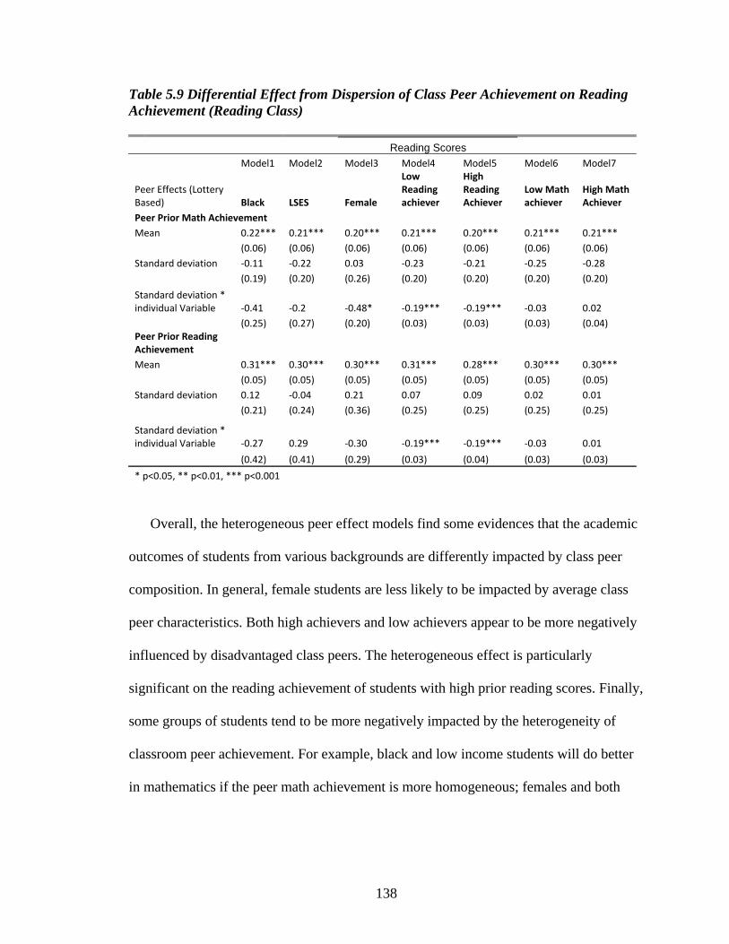
138

Table 5.9 Differential Effect from Dispersion of Class Peer Achievement on Reading Achievement (Reading Class) Reading Scores


Peer Effects (Lottery Based) Black LSES Female



Low Math achiever

High Math Achiever


Mean 0.22*** 0.21*** 0.20*** 0.21*** 0.20*** 0.21*** 0.21***

(0.06) (0.06) (0.06) (0.06) (0.06) (0.06) (0.06)

Standard deviation ‐0.11 ‐0.22 0.03 ‐0.23 ‐0.21 ‐0.25 ‐0.28

(0.19) (0.20) (0.26) (0.20) (0.20) (0.20) (0.20)

Standard deviation * individual Variable ‐0.41 ‐0.2 ‐0.48* ‐0.19*** ‐0.19*** ‐0.03 0.02


Mean 0.31*** 0.30*** 0.30*** 0.31*** 0.28*** 0.30*** 0.30***

(0.05) (0.05) (0.05) (0.05) (0.05) (0.05) (0.05)

Standard deviation 0.12 ‐0.04 0.21 0.07 0.09 0.02 0.01

(0.21) (0.24) (0.36) (0.25) (0.25) (0.25) (0.25)

Standard deviation * individual Variable ‐0.27 0.29 ‐0.30 ‐0.19*** ‐0.19*** ‐0.03 0.01

(0.42) (0.41) (0.29) (0.03) (0.04) (0.03) (0.03)

* p<0.05, ** p<0.01, *** p<0.001

Overall, the heterogeneous peer effect models find some evidences that the academic

outcomes of students from various backgrounds are differently impacted by class peer

composition. In general, female students are less likely to be impacted by average class

peer characteristics. Both high achievers and low achievers appear to be more negatively

influenced by disadvantaged class peers. The heterogeneous effect is particularly

significant on the reading achievement of students with high prior reading scores. Finally,

some groups of students tend to be more negatively impacted by the heterogeneity of

classroom peer achievement. For example, black and low income students will do better

in mathematics if the peer math achievement is more homogeneous; females and both

139

high and low reading achievers will score higher in reading if their reading class peers are

less dispersed in prior math achievement.

Robustness Checks

Following the procedures in last chapter, I also ran a set of models to check if the

strong estimates of class peer effects pick up the effects of some other factors than the

classroom peer characteristics. First, I include the interaction of the treatment indicators

with individual characteristics in the regression to test if peer effects are confounded with

the heterogeneity in treatment responses. However, it turns out that the point estimates of

classroom peer effects become even larger (and remain significant) when the

heterogeneous interaction term is controlled. The results do not support that the estimated

classroom peer effects are proxies for treatment response heterogeneity.

Second and more importantly, I implemented teacher fixed effect model to test if

classroom peer effects are confounded with teacher impacts. One of the challenges faced

by peer effect identification at the classroom level is the non-random matching between

teachers and students within each school. For example, schools may place students with

disciplinary problems with one teacher who is more experienced with misbehaving

students; or schools may assign the best teachers to classes with high performing

students. Therefore, the estimation of classroom peer effects is likely to pick up some

effects of teacher characteristics.52

52 For example, the Florida study by Burk and Sass (2004) finds that adding teacher fixed effect totally overturned the significant estimates of peer influence on student math achievement. They argue that the apparent peer impacts found in other studies may just reflect the endogenous matching between teachers and students within a school.

140

The estimates of classroom peer effect models (on math achievement) with teacher

fixed effect are presented in Table 5.1053. Due to the large amount of data required by

teacher fixed effect models, the standard errors of the peer effect estimates arise.

However, the point estimates of some major classroom peer characteristics, including

percent black students, percent low income students, average peer math achievement,

average peer reading achievement, and average peer disciplinary records become even

larger and still remain statistically significant. Therefore, there is little evidence that the

large estimated effects of classroom peers are signals for teacher qualities or the

endogenous matching between teachers and students.

Table5.10 Average Class Peer Effects on Math Achievement (Teacher Fixed Effect) Math Scores

Independent Variables Model1 Model2 Model3 Model4 Model5 Model6 Model7 Model8 Model9 Model10


Academic Yes Yes Yes Yes Yes Yes Yes Yes Yes Yes

Non‐Academic Composite Yes Yes Yes Yes Yes Yes Yes Yes Yes Yes


Black (proportion) ‐0.96***

(0.24)

Low SES (proportion) ‐1.39***

(0.27)

Female (proportion) 0.26

(0.36)

Hispanic (proportion) ‐3.59

(2.49)

Special ED (proportion) ‐1.18*

(0.54)

ELL (proportion) 6.45

(3.57)

Grade 4 Math (Mean) 0.42**

(0.10)


(0.09)

53 The findings from the teacher fixed effect models on reading achievement are quite similar, except that the estimate of average peer disciplinary infraction effect is larger and significant.

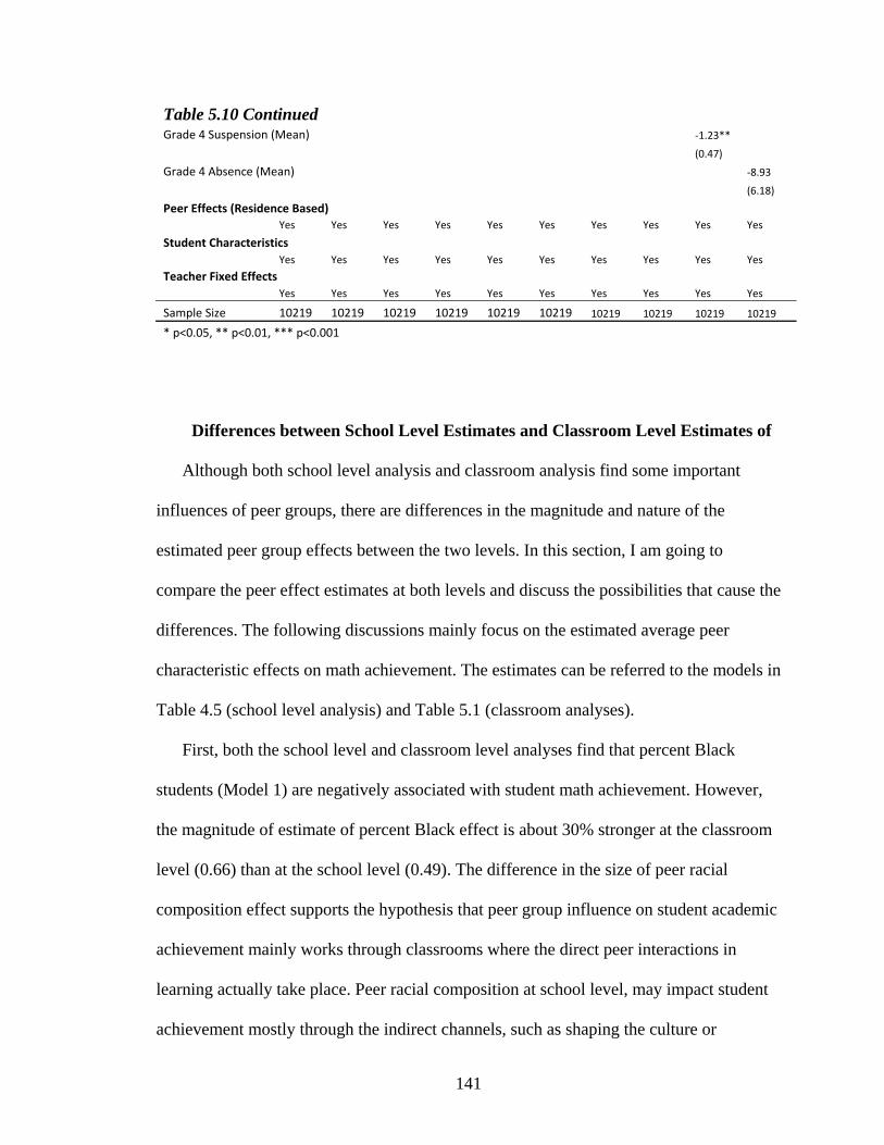
141

Table 5.10 Continued

Grade 4 Suspension (Mean) ‐1.23**

(0.47)


(6.18)





Teacher Fixed Effects


Sample Size 10219 10219 10219 10219 10219 10219 10219 10219 10219 10219

* p<0.05, ** p<0.01, *** p<0.001

Differences between School Level Estimates and Classroom Level Estimates of

Although both school level analysis and classroom analysis find some important

influences of peer groups, there are differences in the magnitude and nature of the

estimated peer group effects between the two levels. In this section, I am going to

compare the peer effect estimates at both levels and discuss the possibilities that cause the

differences. The following discussions mainly focus on the estimated average peer

characteristic effects on math achievement. The estimates can be referred to the models in

Table 4.5 (school level analysis) and Table 5.1 (classroom analyses).

First, both the school level and classroom level analyses find that percent Black

students (Model 1) are negatively associated with student math achievement. However,

the magnitude of estimate of percent Black effect is about 30% stronger at the classroom

level (0.66) than at the school level (0.49). The difference in the size of peer racial

composition effect supports the hypothesis that peer group influence on student academic

achievement mainly works through classrooms where the direct peer interactions in

learning actually take place. Peer racial composition at school level, may impact student

achievement mostly through the indirect channels, such as shaping the culture or

142

environment of the schools (e.g., low expectations and fewer resources in a school with

disproportional black students). However, peer racial composition at classroom level, in

addition to the indirect influence such as teacher expectations, may also have direct

impact on student achievement through the interactions between students. For example,

black students are more likely to have disciplinary problems (as found in next chapter),

which can directly impact student learning if the disruptive behavior happens in the

classroom.

Second, while there is little evidence that the percentage of low income students

(model 2) at school level impacts student math achievement, the estimated effect at the

classroom level is large and significant. The same patterns are also found from model 7

and model 8 --- school level estimates of average peer academic abilities (in both

subjects) do not show significant influence on student math achievement, but the

classroom level estimates are positive and significant. One possibility is due to the

tracking practice in middle schools. As suggested by many studies (e.g., Gamoran, 1986;

Oaks, 1990; Argys, Rees & Brewer, 1996; Mickelson, 2001), students are often tracked

in schools (especially in middle and high schools). Therefore, if disadvantaged students,

such as low SES students or students with low academic abilities, are grouped with other

disadvantaged students for classes no matter what school they attend (regardless of the

school type or the average school peer characteristics), then the school level peer

composition may only have a moderate or no influence on student outcomes. Moreover,

the estimated differences between school level and classroom level further suggest that

the causal relationship between peer groups and student achievement mostly comes from

classrooms where students directly interact with each other on learning activities.

143

Third, although school level analysis finds that high percent female students decrease

individual math scores, the significance vanishes at the classroom level (Model 3).

Although it might be true that schools with more female students have relatively lower

expectations on math achievement and put more emphasis on reading or language arts

classes, I would not draw the conclusion from the school level estimate that there is a

strong and negative causal relationship between percent female students and average

student math achievement. As I mentioned in the previous chapter, because the analytical

strategy in this paper identifies peer effect from the average difference in peer

characteristics between the treatment group and the control group, the small gap in school

gender composition between the two groups is likely to yield a large coefficient on the

peer variable percent female students. However, although it may also be true that there

are low expectations and motivations in a female dominate math class, the negative

impact can be canceled out because there are fewer classroom disruptions.

Fourth, the school level models find significant and positive effects from percent

school special education students and percent ELL students. In our data, many of the

special education and ELL lottery participants chose to attend neighborhood schools even

when they won the lottery of the academic magnet school, which may signal the

perceptions of certain school qualities of some neighborhood schools, such as good

special education or ELL programs, or teachers more experienced with special need or

ELL students. However, I still would not conclude that the causal relationship between

student achievement and school special education students or ELL students is strongly

positive. In fact, the classroom estimate of percent special education students tells a

totally different story: having more students with special needs in a class reduces average

144

student math achievement in middle school. For example, when the instructor has to slow

down her class pace or spend disproportional time teaching students with learning

disabilities, it will likely have a negative impact on other students in the same classes

regardless of their own academic abilities. Interestingly, the classroom heterogeneous

peer effect model finds that in our sample, the negative influence of percent special

education students mainly works on the lottery participants who are also special

education students. This is not surprising because the special education lottery

participants perform much better in both subjects than other special education students in

the same district.54 Therefore, if special education lottery participant are put in a special

education class where most of other students are at extremely low academic levels55, it is

very likely that they are going to achieve lower than what they could do in a class with

regular students. Moreover, although the classroom estimate of percent ELL student is

also positive and very close to the school level estimate in magnitude, the impact of

having more ELL peers in the same classroom might work differently from the impact of

school level ELL peers. Note that in our sample, ELL lottery participants outperform

other students in mathematics56. Due to the tracking policy in middle school, having more

ELL classmates may also signal a high average class math achievement in the magnet

schools where all ELL students are enrolled through admission lotteries.

54 The average prior scores for special education lottery participants are 620 (math) and 646 (reading); and the average prior scores for non-lottery participant special education students are 572 (math) and 585 (reading). The average scores for the special education lottery participants are even higher than the average scores for the non lottery participant regular students (623 in math, 635 in reading). 55 This is most likely to happen in neighborhood schools where many special education lottery participants choose to attend and other special education enrollees (the majority) did not participated in the magnet school lotteries. 56 Although the average prior math achievement for ELL lottery participants is slightly lower than other lottery participants, they achieve higher math scores in middle schools than other lottery participants in our sample.

145

Fifth, average peer disciplinary infractions only show significantly negative impact

on student achievement at classroom level (model 9). One possibility that causes the

insignificant school level estimate is also due to the school tracking policy. If students

with behavioral problems are often placed in the same class (maybe because the teacher

is experienced with disruptive students), it is likely to find little impact from the average

school level disciplinary variable. The big difference in the estimates of average peer

disciplinary records at both levels again suggests that peer group influence on student

achievement mostly comes from classroom level instead of school level.

Finally, although the estimates of average peer absence behavior are not statistically

significant at both school and classroom levels, the signs of the coefficients are opposite.

Moreover, the heterogeneous peer effect models at the classroom level (Table 5.5) find

that some groups of students, such as non-Blacks, high income students, boys, and

students at the two ends of achievement distributions, are negatively impacted by average

peer absence rate (significant at 5% level). For example, if the class teacher has to spend

disproportional time helping a frequent absent student catch up with school work, it will

definitely slow down the study of other students in the same class. However, this negative

impact is unlikely to be spread to students in other classes of the same school.

Overall, the comparison of peer effect estimates between school level and classroom

level suggests that stronger and direct influence of peers on student academic

achievement comes from classrooms where the direct peer interaction in learning mostly

takes place. The school level peer composition, however, has a relatively moderate

impact on student academic outcomes through shaping school culture and atmosphere.

146

CHAPTER VI

PEER EFFECTS ON BEHAVIORAL OUTCOMES --- RESULTS FROM BOTH SCHOOL AND CLASSROOM LEVEL ANALYSES

Although a large body of research has extensively examined the presence of peer

effects in education, most studies have focused on student academic outcomes. Due to

data limitations, the question of whether peers influence student non-scholastic outcomes

in school is much less studied in literature. In this project, I am able to derive two

behavioral outcome variables from the district admission data. The two outcomes of

interest include student discipline and attendance, which are considered as important

indicators of student social engagement and participation in schools. (Rowley, 2005)

This chapter seeks to explore the impacts of peer groups on student disciplinary and

attendance behaviors in school. The first part of this chapter presents some descriptive

statistics of the two outcome variables. The second part reports the magnet school

treatment effects, with no peer variables controlled. The following sections are organized

to answer the three research questions of: (1) the influence on peer behaviors from

average peer composition; (2) the impact from the dispersion of peer composition; and

(3) the heterogeneous peer effects. Different from previous two chapters, the regression

results from both school and classroom analyses will be reported and discussed together

in this chapter.

147

Descriptive Statistics of the Outcomes Variables

Disciplinary Infraction

The district discipline data keep the records of the disciplinary actions given to a

student as a consequence to his/her misconducts. The actions are taken based on the

severity of student behavior, including less severe punishments, such as warning, call to

parents, or corporal punishment, and severe punishments, like suspension (both in school

and out of school) and expulsion.57 While well behaved students do not have any record

in the discipline data, many students experienced more than one disciplinary action in a

given year. To measure student disciplinary infractions, I coded two variables from these

records: annual number of times punished, which sums all disciplinary actions for every

student in each year; and annual number of times suspended, counting only in-school and

out-of-school suspensions. A zero value is given to the students who did not receive any

disciplinary actions in the school year.

The current value of the discipline variable is used as dependent variable to measure

student behavior in middle school. The 4th grade value of the discipline variable is

included in the regression models as an independent variable, and is also aggregated at

both school and classroom level to form the peer behavioral variable. I ran the regression

analyses on both discipline variables (total punishment numbers and total suspension

numbers) and obtained very similar conclusions. Following Figlio’s 2005 study in which

suspension is used as the outcome of interest, I report only the results for the suspension

variable in this chapter.

57 Since there are only 2 students (among 5 cohorts) expelled from middle schools in our data, I did not include the expulsion variable in discipline measures.

148

Table 6.1 Descriptive Statistics of the Dependent Variable: Number of Suspensions Suspension Numbers (per student per year)

Grade 5 Grade 6 Grade 7 Grade 8



All 0.25 0.94 0.35 1.21 0.61 1.81 0.72 1.87

Academic

Participants 0.14 0.61 0.20 0.92 0.32 1.13 0.39 1.12 Enrollees 0.11 0.54 0.10 0.45 0.10 0.54 0.18 0.63




Participants 0.31 1.05 0.42 1.32 0.76 2.07 0.88 2.12

Enrollees 0.29 1.02 0.43 1.42 0.75 1.96 0.80 1.69



*Counted only students who were in the system as 4th graders in the lottery year.

Table 6.1 presents the descriptive results of the suspension variable for lottery

participants. Clearly, the disciplinary infractions increase as the students progress through

grades. The biggest jump is between 6th grade and 7th grade --- the average number of

suspensions for 7th graders is almost double the number for 6th graders. While this

suggests that older students are more likely to have disciplinary problems in school, it

may also reflect that schools become stricter with student behavioral problems in higher

grades and issue more suspensions. Academic magnet school enrollees appear to receive

fewer suspensions than their counterpart students enrolled in neighborhood schools; this

pattern is also true of non-academic magnet lottery participants. The large standard

deviation of this variable suggests that there is a great variation in behaviors among all

lottery participants.

149

Absence Rate

The district keeps a daily base attendance record for each student. For each required

school day, I code the absence variable as 1 if a student was absent (either unexcused or

excused), 0 otherwise. I then sum the values of the absence variable across the days in the

school year that the student was enrolled in the district. The total is then divided by the

days enrolled for each student to calculate the annual absence rate.

Similar to other outcome variables, the current value of this variable enters the

regression model as a dependent variable. The lagged measure (4th grade) of this variable

is employed to form the peer variable measuring peer attendance behavior, and is also

included as an individual control in the regression.

Table 6.2 Descriptive Statistics of the Dependent Variable: Absence Rate

Annual Absence Rate

Grade 5 Grade 6 Grade 7 Grade 8

Absence Rate



All 0.03 0.05 0.03 0.04 0.04 0.05 0.04 0.05

Academic

Participants 0.03 0.04 0.03 0.03 0.03 0.05 0.04 0.04

Enrollees 0.03 0.03 0.03 0.03 0.03 0.03 0.03 0.03




Participants 0.03 0.04 0.03 0.05 0.04 0.05 0.04 0.05

Enrollees 0.03 0.03 0.03 0.03 0.03 0.04 0.03 0.03

Enrollees in Other Magnet Schools 0.03 0.03 0.03 0.03 0.03 0.03 0.03 0.03 Enrollees in Non‐Magnet Schools 0.04 0.06 0.04 0.06 0.04 0.06 0.05 0.06

*Counted only students who were in the system as 4th graders in the lottery year.

150

As shown in Table 6.2, the average absence rate of the lottery participants is 0.035

across grades. The difference in average absence rate between magnet school enrollees

and lottery participants enrolled in other schools is small --- the average gap is 0.01 for

both academic and non-academic magnet schools. If all lottery participants were enrolled

in the district for a full school year (175 school days)58, a difference of 0.01 in absence

rate would mean that lottery participants enrolled in neighborhood schools were absent

1.75 days more than the winners enrolled in the magnet programs. There is also more

variation in attendance rate among the lottery losers in non-magnet schools than among

the magnet school enrollees.

Magnet School Treatment Effects

Although academic outcome improvement is often used to evaluate the effectiveness

of school choice programs, many studies also suggest that choice schools outperform

their counterpart neighborhood schools in issues like student behavior and parental

satisfaction (e.g., Cullen et al., 2003; Peterson, 1998; Smrekar and Goldring, 1999). This

section examines whether the magnet schools in the district reduce student misconduct in

middle schools and improve student attendance. The regression strategy is the same as

the one used in the academic achievement models.

Disciplinary Infractions

Table 6.3 presents the estimated treatment effects on student disciplinary infractions

from the models using both the small sample and the large sample. When I estimate the

model using the sample of 5th and 6th graders, I do not find significant treatment effects 58 The school year length varies across years, from 169 to 180 days.

151

for either the academic or non-academic magnet schools. However, results for the large

sample indicate that enrolling in a magnet school substantially reduces the number of

suspensions. The estimated treatment effect is larger for the non-academic magnet

composite --- with all individual background variables held constant, students who enroll

in the non-academic magnet composite schools are likely to receive 0.4 fewer

suspensions than lottery losers who attend a neighborhood school.

The second panel of Table 6.3 shows the coefficients on individual characteristics.

Compared to other students, black students, special education program students, and

students from low SES families are more likely to receive disciplinary actions. Female

students, and students with higher prior test scores, not surprisingly, appear to behave

better. Also as it is expected, prior behavioral outcome is strongly correlated to student

current behavior problems in middle school.

Table 6.3 Magnet School Treatment Effects on Disciplinary Infractions

Suspension Numbers

First 2 Grades All 4 Grades

Independent Variables Academic Magnet Treatment Academic ‐0.043 ‐0.262*** (0.06) (0.07) Non‐Academic Magnet Treatment Composite 0.066 ‐0.401* (0.14) (0.19) Student Characteristics

Black 0.229*** 0.375*** (0.03) (0.04) Hispanic 0.035 0.048 (0.11) (0.11)

Special Education 0.397*** 0.561***

(0.07) (0.07)

Low SES 0.198*** 0.348***

(0.03) (0.03) ELL ‐0.196 ‐0.13 (0.14) (0.17)

Female ‐0.190*** ‐0.245***

(0.03) (0.03)

152

Table 6.3 Continued

Grade 4 Reading ‐0.051* ‐0.058**

(0.02) (0.02)

Grade 4 Math ‐0.062** ‐0.069***

(0.02) (0.02)

Grade 4 Absence 0.61 0.975

(0.48) (0.50)

Grade 4 Suspension 0.593*** 0.669***

(0.04) (0.04)

Over-Identification Test 0.06 0.3

N 6558 12286

* p<0.05, ** p<0.01, *** p<0.001

Absence Rate

The estimated magnet school treatment effects on student attendance are reported in

Table 6.4. In neither sample do I find significant magnet school effects on student

absence rate. The coefficients on individual characteristics suggest that with all other

factors held constant, blacks, girls, and ELL students are less likely to be absent from

schools. Special education program students and students from low SES background,

however, have higher absence rates than other students. As expected, students with

higher prior math scores show better attendance behavior, and students who were more

often absent in 4th grade continue to have higher absence rates in middle school.

153

Table 6.4 Magnet School Treatment Effects on Attendance Behavior

Absence Rate

First 2 Grades All 4 Grades

Independent Variables Model1 Model2 Academic Magnet Treatment Academic ‐0.005 ‐0.004 (0.00) (0.00) Non‐Academic Magnet Treatment Composite 0.000 ‐0.003 (0.01) (0.01) Student Characteristics Black ‐0.008*** ‐0.008*** (0.00) (0.00) Hispanic 0.007 0.002 (0.00) (0.00) Special Education 0.011*** 0.011*** (0.00) (0.00)

Low SES 0.005*** 0.010*** (0.00) (0.00) ELL ‐0.015** ‐0.013* (0.01) (0.01) Female ‐0.002* ‐0.002** (0.00) (0.00) Grade 4 Reading ‐0.001 0.001 (0.00) (0.00) Grade 4 Math ‐0.002** ‐0.003*** (0.00) (0.00)

Grade 4 Absence 0.603*** 0.587*** (0.02) (0.01)

Grade 4 Suspension ‐0.000 0.002

(0.00) (0.00)

Over-Identification Test 0.34 0.31

N 6558 12286

* p<0.05, ** p<0.01, *** p<0.001

Impacts from Average Peer Characteristics

This section presents the estimated effects of average peer characteristics on student

discipline and attendance behaviors. As in the previous two chapters, I present the results

from the large sample models only.


1. School Level Analysis

154

The coefficients on school level peer characteristics are reported in Table 6.5. Each

peer characteristic is examined separately in Model 1 to Model 10, while all peer

variables are incorporated in Model 11.

The top 2 rows of Table 6.5 present the estimated magnet school treatment. These

effects continue to be negative, which indicates that students in the magnet schools have

fewer behavioral problems even with peer variables controlled. Indeed, the magnet

school treatment effects are even stronger in many equations.

Many of the estimated effects have unexpected coefficients. First, Increases in the

percent low income (column 2), percent Hispanic (column 4), and percent special

education students (column 5), are associated with fewer incidences of measured

misbehavior (measured by the numbers suspended). Second, average school peer

academic achievement (measured by 4th grade test scores in both math and reading) is

positively correlated with measured misbehavior. A 1 point (in standardized scores)

difference in average peer prior math achievement produces 1.5 suspensions. Third,

students whose peers were more frequently absent appear to behave better in middle

school. Finally, model 9 suggests that there is no significant correlation between school

peer prior disciplinary records and individual behavioral outcomes in middle schools.

There are some possible reasons for the unexpected coefficients on the school level

peer variables. First, although district has a uniform discipline code, it is the school that

takes disciplinary actions based on student behavior. The way in which each school deals

with misbehaving students can vary: the same kind of misconduct may receive different

consequences in different schools. Second, it is possible that the student body

composition influences a school’s discipline decisions. For example, a neighborhood

155

school with a higher proportion of low-income and low achieving students may be less

willing to punish a lottery participant for his misbehavior just because this student

performs and behaves better than other students in this school. However, if this student

enrolled in a magnet school, it is less likely that he will get an exemption.

Although most peer characteristics have a significant influence on individual

behaviors in the single variable models, this is true less often in column 11 where all peer

characteristics are included. Due to the high collinearity among the peer variables, the

estimated effects of most peer characteristics are insignificant. As shown in Column 11,

there are three significant coefficients. The estimated effects of percent female students

and average peer math achievement are positive and significant at 5% statistical level.

Average peer prior disciplinary record shows a strong and positive impact on individual

behaviors while all school peer characteristics are controlled.

Six residence based peer attributes show significant impact on student disciplinary

infractions. Although the estimates of residence based peer effects are less sizeable than

the estimates of lottery based peer effects, they all have expected coefficient signs. In

none of the 11 models does the inclusion of school peer characteristics overturn the

magnet school effects; rather, the treatment effects are even bigger in most models with

school peer variables controlled.

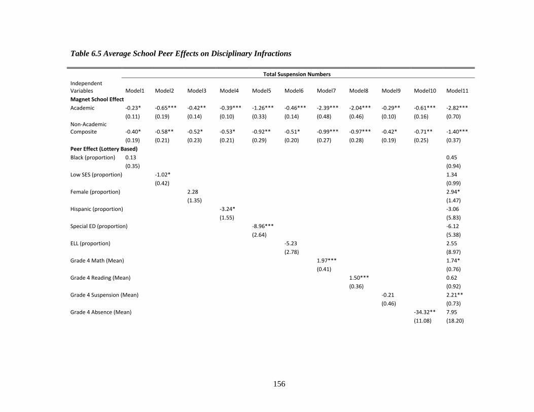
156

Table 6.5 Average School Peer Effects on Disciplinary Infractions Total Suspension Numbers



Academic ‐0.23* ‐0.65*** ‐0.42** ‐0.39*** ‐1.26*** ‐0.46*** ‐2.39*** ‐2.04*** ‐0.29** ‐0.61*** ‐2.82***

(0.11) (0.19) (0.14) (0.10) (0.33) (0.14) (0.48) (0.46) (0.10) (0.16) (0.70)

Non‐Academic Composite ‐0.40* ‐0.58** ‐0.52* ‐0.53* ‐0.92** ‐0.51* ‐0.99*** ‐0.97*** ‐0.42* ‐0.71** ‐1.40***

(0.19) (0.21) (0.23) (0.21) (0.29) (0.20) (0.27) (0.28) (0.19) (0.25) (0.37)


Black (proportion) 0.13 0.45

(0.35) (0.94)

Low SES (proportion) ‐1.02* 1.34

(0.42) (0.99)

Female (proportion) 2.28 2.94*

(1.35) (1.47)

Hispanic (proportion) ‐3.24* ‐3.06

(1.55) (5.83)

Special ED (proportion) ‐8.96*** ‐6.12

(2.64) (5.38)

ELL (proportion) ‐5.23 2.55

(2.78) (8.97)

Grade 4 Math (Mean) 1.97*** 1.74*

(0.41) (0.76)

Grade 4 Reading (Mean) 1.50*** 0.62

(0.36) (0.92)

Grade 4 Suspension (Mean) ‐0.21 2.21**

(0.46) (0.73)

Grade 4 Absence (Mean) ‐34.32** 7.95

(11.08) (18.20)

157

Table 6.5 (Continued) Peer Effects (Residence Based)

Black (proportion) 0.22* 0.10

(0.10) (0.14)

Low SES (proportion) 0.36*** 0.06

(0.10) (0.23)


(0.31) (0.34)

Hispanic (proportion) 0.36* 0.44

(0.17) (0.23)

Special ED (proportion) 0.67*** 0.20

(0.18) (0.25)

ELL (proportion) 0.05 ‐0.23

(0.13) (0.18)

Grade 4 Math (Mean) ‐0.27*** ‐0.70**

(0.05) (0.23)

Grade 4 Reading (Mean) ‐0.22*** 0.45

(0.05) (0.23)

Grade 4 Suspension (Mean) 0.12 ‐0.55**

(0.15) (0.18)

Grade 4 Absence (Mean) 4.64 1.88

(2.42) (3.50


Yes Yes Yes Yes Yes Yes Yes Yes Yes Yes yes


Sample Size 12195 12195 12195 12195 12195 12195 12195 12195 12195 12195 12195

* p<0.05, ** p<0.01, *** p<0.001

158


Although most middle school students in the district rotate through classes on

different subjects, a student’s classroom peers are relatively stable across subjects given

that many schools practice tracking or ability grouping59. Therefore, the interactions

between one student and his classmates are more frequent than the interactions with the

average school peers; and the impacts from one’s class peers are expected to be stronger

and more meaningful even on discipline and attendance outcomes.

Because the classroom peer variables are subject based, there are two sets of peer

variables from math classes and reading/language arts classes. I ran separate models

using peers in both subjects and obtained very similar estimates of peer effects. Here I

report the results for only math class peers. 60

Table 6.6 presents estimates of models that include classroom peer variables. The

estimated effects of peer characteristics at the classroom level are quite different from

those at school level and all of the significant coefficients have the expected signs. A

higher proportion of black and low SES classmates is associated with more disciplinary

infractions: a student is likely to receive 1 more suspension if he moves from a class with

no low income peers to a class with 80% low income students61. Second, peer academic

ability (measured by prior reading achievement) appears to decrease individual

misdemeanors. A 1 point increase in peer prior reading scores (standardized scores)

yields a 0.4 decrease in student suspension times. Third, classmates’ prior disciplinary

records are strongly correlated with individual behavioral problems in middle school. The

59 In some schools, there is less ability-grouping in 5th and 6th grades, and students tend to stay with the same group of peers for all subjects just like elementary schools. 60 The results from the reading class peer models are included in Appendix F. 61 The estimated effect is quite large given that about 78% lottery participants never received any suspension during the years of investigation.

159

estimated effect of peer’s prior behavioral problems is very substantial --- if every peer in

the same class received 1 more suspension in 4th grade, the average class number

suspended in middle school increase by 1.8. Finally, being with classmates with past

history of higher absence rates also increases individual misconduct as measured by

suspension numbers. Overall, the single variable models find significant and expected

peer effects on student disciplinary infractions from both peer racial/SES composition

variables and peer prior behaviors.

Model 11 incorporates all classroom peer characteristics. Most peer variables are

individually insignificant in the full model except peers’ prior absence rate, which

remains positive and weakly significant. Some of this may be due to the collinearity

among the class peer variables, which increase the standard errors.

In an equation where a classroom peer characteristic has a significant influence on

student behavior, magnet school treatment effects are insignificant. One exception is

model 9, where the estimated treatment effect of the academic magnet program remains

negative and significant, but less sizeable than the estimate in Table 6.3. When the model

controls all peer characteristics, the point estimate of the non-academic magnet effect

falls nearly to zero.

160

Table 6.6 Average Classroom Peer Effects on Disciplinary Infractions (Math Class)

Total Suspension Numbers



Academic ‐0.10 0.05 ‐0.28** ‐0.36*** ‐0.25** ‐0.33* ‐0.13 0.05 ‐0.18* ‐0.08 0.13

(0.08) (0.11) (0.09) (0.10) (0.09) (0.13) (0.12) (0.13) (0.08) (0.11) (0.17) Non‐Academic Composite ‐0.33 ‐0.21 ‐0.36 ‐0.45* ‐0.35 ‐0.39 ‐0.33 ‐0.24 ‐0.33 ‐0.09 0.02

(0.20) (0.20) (0.20) (0.21) (0.21) (0.21) (0.20) (0.21) (0.20) (0.24) (0.26)


Black (proportion) 0.96*** 0.85

(0.21) (1.01)

Low SES (proportion) 1.23*** 0.76

(0.24) (0.79)


(0.57) (0.62)

Hispanic (proportion) ‐3.05 ‐4.12

(1.64) (2.56)

Special ED (proportion) 1.30 0.83

(0.82) (1.24)

ELL (proportion) ‐1.92 3.63

(2.95) (5.97)

Grade 4 Math (Mean) ‐0.22 0.97

(0.13) (0.52)

Grade 4 Reading (Mean) ‐0.42*** ‐0.51

(0.11) (0.33)

Grade 4 Suspension (Mean) 1.75*** 0.60

(0.46) (0.69)

Grade 4 Absence (Mean) 28.37** 36.48*

(9.58) (16.68)




Yes Yes Yes Yes Yes Yes Yes Yes Yes Yes yes


Sample Size 10369 10369 10369 10369 10369 10369 10368 10368 10368 10368 10368

* p<0.05, ** p<0.01, *** p<0.001

161

The results from both school and classroom level analyses on student discipline

problems are very interesting. Although the school level results suggest many

unfavorable peer attributes decreasing student misdemeanors, the classroom level results

find the opposite. Moreover, classroom analyses find strong and expected effects from

peer prior achievement and behaviors. Again, the results suggest that the stronger and

direct impacts of peer group effects come from classroom level, even on individual

disciplinary outcomes. The estimates of school level peer effects, in this case, reflects

more about how school student composition impact one’s chances of receiving

disciplinary actions (suspensions, as measured in this section).

Attendance Behavior


Table 6.7 reports the effects of school level peers on student attendance behavior.

Only one peer characteristic is found significantly correlated with student attendance

behavior: peers with a history of behavioral problems tend to increase the individual

absence rate in middle schools. Specifically, the coefficient suggests that a student will be

absent for 2.5 more days from school if peer prior suspensions increase by 0.5 on

average.

Several residence-based peer characteristics have shown significant associations with

student absence rate. Students who are from a neighborhood with more low SES families,

or more Hispanic and ELL peers, or more special education peers, are more likely to be

absent from schools than other students. Residence-based peer math achievement is

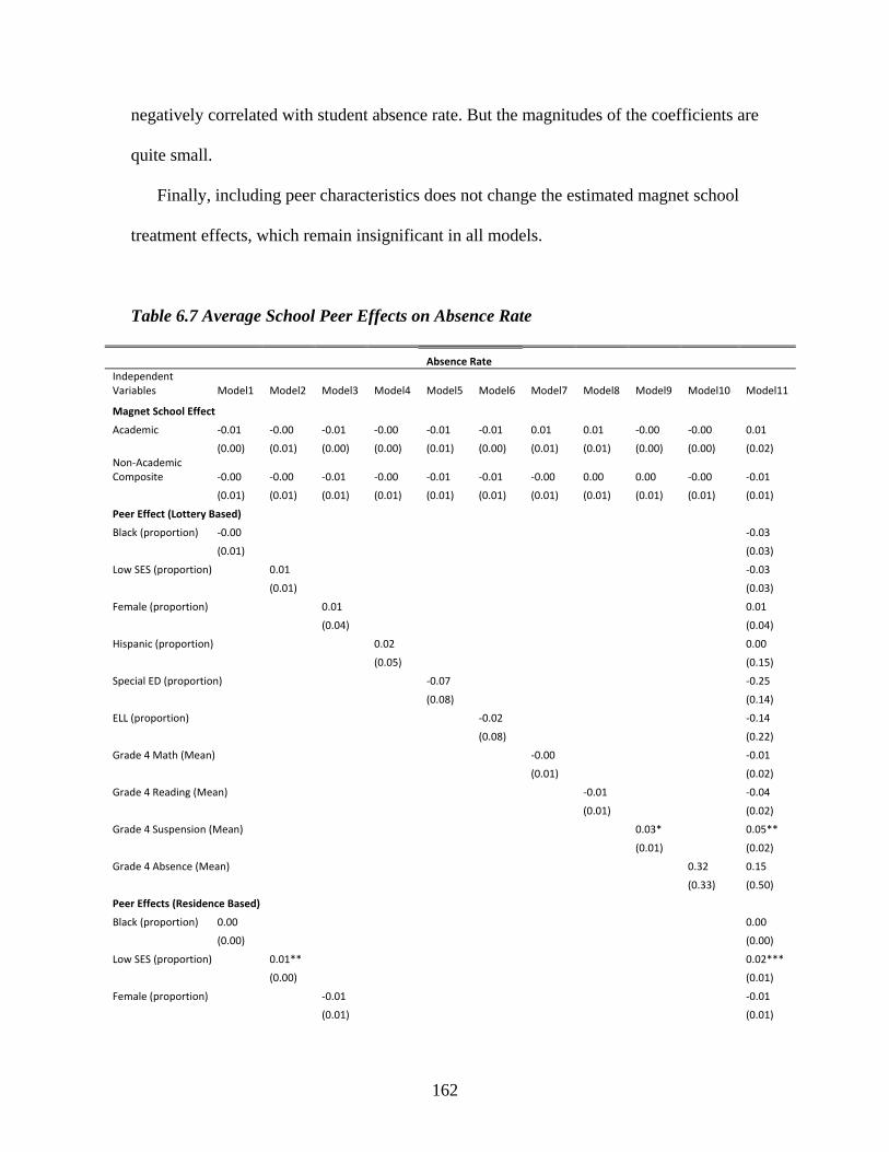
162

negatively correlated with student absence rate. But the magnitudes of the coefficients are

quite small.

Finally, including peer characteristics does not change the estimated magnet school

treatment effects, which remain insignificant in all models.

Table 6.7 Average School Peer Effects on Absence Rate

Absence Rate



Academic ‐0.01 ‐0.00 ‐0.01 ‐0.00 ‐0.01 ‐0.01 0.01 0.01 ‐0.00 ‐0.00 0.01

(0.00) (0.01) (0.00) (0.00) (0.01) (0.00) (0.01) (0.01) (0.00) (0.00) (0.02) Non‐Academic Composite ‐0.00 ‐0.00 ‐0.01 ‐0.00 ‐0.01 ‐0.01 ‐0.00 0.00 0.00 ‐0.00 ‐0.01

(0.01) (0.01) (0.01) (0.01) (0.01) (0.01) (0.01) (0.01) (0.01) (0.01) (0.01)


Black (proportion) ‐0.00 ‐0.03

(0.01) (0.03)


(0.01) (0.03)


(0.04) (0.04)


(0.05) (0.15)

Special ED (proportion) ‐0.07 ‐0.25

(0.08) (0.14)

ELL (proportion) ‐0.02 ‐0.14

(0.08) (0.22)

Grade 4 Math (Mean) ‐0.00 ‐0.01

(0.01) (0.02)

Grade 4 Reading (Mean) ‐0.01 ‐0.04

(0.01) (0.02)

Grade 4 Suspension (Mean) 0.03* 0.05**

(0.01) (0.02)

Grade 4 Absence (Mean) 0.32 0.15

(0.33) (0.50)



(0.00) (0.00)

Low SES (proportion) 0.01** 0.02***

(0.00) (0.01)


(0.01) (0.01)

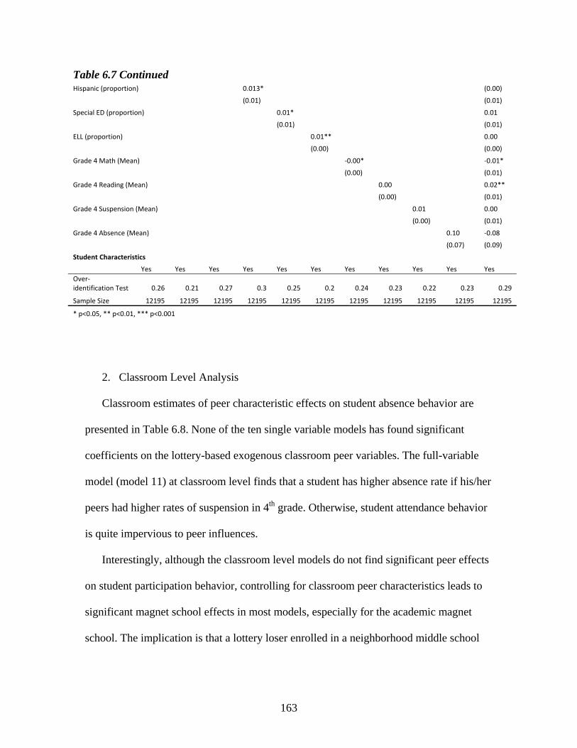
163

Table 6.7 Continued

Hispanic (proportion) 0.013* (0.00)

(0.01) (0.01)

Special ED (proportion) 0.01* 0.01

(0.01) (0.01)

ELL (proportion) 0.01** 0.00

(0.00) (0.00)

Grade 4 Math (Mean) ‐0.00* ‐0.01*

(0.00) (0.01)

Grade 4 Reading (Mean) 0.00 0.02**

(0.00) (0.01)

Grade 4 Suspension (Mean) 0.01 0.00

(0.00) (0.01)

Grade 4 Absence (Mean) 0.10 ‐0.08

(0.07) (0.09)




Sample Size 12195 12195 12195 12195 12195 12195 12195 12195 12195 12195 12195

* p<0.05, ** p<0.01, *** p<0.001


Classroom estimates of peer characteristic effects on student absence behavior are

presented in Table 6.8. None of the ten single variable models has found significant

coefficients on the lottery-based exogenous classroom peer variables. The full-variable

model (model 11) at classroom level finds that a student has higher absence rate if his/her

peers had higher rates of suspension in 4th grade. Otherwise, student attendance behavior

is quite impervious to peer influences.

Interestingly, although the classroom level models do not find significant peer effects

on student participation behavior, controlling for classroom peer characteristics leads to

significant magnet school effects in most models, especially for the academic magnet

school. The implication is that a lottery loser enrolled in a neighborhood middle school

164

tends to be absent from school for 2 more days even if he/she attends a class whose peers

are identical to the class peers in the academic magnet.

Table 6.8 Average Classroom Peer Effects on Absence Rate (Math Class)

Absence Rates



Academic ‐0.01** ‐0.00 ‐0.01** ‐0.00** ‐0.01** ‐0.00 ‐0.01* ‐0.01 ‐0.00** ‐0.01** ‐0.01*

(0.00) (0.00) (0.00) (0.00) (0.00) (0.00) (0.00) (0.00) (0.00) (0.00) (0.00) Non‐Academic Composite ‐0.01 ‐0.01 ‐0.01* ‐0.01 ‐0.01* ‐0.01 ‐0.01* ‐0.01 ‐0.01 ‐0.01* ‐0.01

(0.00) (0.01) (0.01) (0.01) (0.01) (0.01) (0.01) (0.01) (0.00) (0.01) (0.01)



(0.01) (0.03)


(0.01) (0.02)


(0.01) (0.02)


(0.04) (0.07)


(0.02) (0.03)

ELL (proportion) 0.08 0.20

(0.07) (0.15)

Grade 4 Math (Mean) 0.00 0.02

(0.00) (0.01)

Grade 4 Reading (Mean) 0.00 ‐0.00

(0.00) (0.01)

Grade 4 Suspension (Mean) 0.02 0.04*

(0.01) (0.02)

Grade 4 Absence (Mean) ‐0.34 ‐0.05

(0.24) (0.43)






Sample Size 10369 10369 10369 10369 10369 10369 10368 10368 10368 10368 10368

* p<0.05, ** p<0.01, *** p<0.001

165


In this section, I examine whether the variance of peer academic abilities and peer

behavioral outcomes impacts student discipline and participation behaviors.



In Table 6.9, peer heterogeneity is measured as the standard deviation of prior peer

test scores (in math and reading), prior suspensions, and prior absence rate. Since the

conclusions regarding magnet school effects and the residence-based peer variables are

very similar to previous findings, Table 6.9 reports only the coefficients on the

exogenous peer variables (means and standard deviations).

Columns 1-2 show the effect of peer achievement. The coefficient on the mean is

positive, but the coefficient on the standard deviation is negative. The implication is that

a lottery participant tends to have fewer measured misbehaviors (indicated by fewer

suspensions received by the student) in a school where there is a greater variation in

student academic ability. Recall my hypothesis that the misbehavior of a lottery

participant enrolled in a neighborhood school may be overlooked because he performs

better than his peers, while the participants enrolled in a magnet school are less lucky

because students in the magnet school are more alike (e.g., all high performers). The

negative coefficient on the standard deviation of peer achievement lends support to this

explanation --- more dispersion in peer ability is associated with less individual

disciplinary infractions as measured by number of suspensions.

166

Table 6.9 Impacts from Dispersion of Peer Characteristics on Disciplinary Infractions (School Level)

Total Suspension Numbers



Yes Yes Yes Yes



(0.29)


(0.35)


(1.07)

Grade 4 Absence (Mean) ‐27.77*

(13.53)


Grade 4 Math (Standard Deviation) ‐1.26***

(0.33)

Grade 4 Reading (Standard Deviation) ‐1.63***

(0.32)


(0.40)


(5.44)


Yes Yes Yes Yes


Yes Yes Yes Yes


Sample Size 12192 12192 12192 12192

* p<0.05, ** p<0.01, *** p<0.001

Neither the mean nor the standard deviation of prior peer suspensions is significantly

associated with student disciplinary infractions in middle school. Moreover, model 4

suggests no significant effect from the heterogeneity in peer attendance behavior on

student disciplinary infractions, although the estimated effect from average peers

attendance rate is still negative and significant.

167


The results from the classroom level dispersion models are presented in Table 6.10.

The heterogeneity of peer academic abilities (Model1 and model 2) does not exert

significant impact on individual discipline behaviors, nor does its inclusion alter the

coefficients on mean peer characteristics.

There is no evidence that the dispersion of peer disciplinary infractions at the

classroom level has any significant impact on individual behaviors. However, controlling

for the dispersion term overturned the effect of the average peer disciplinary record. This

again is due to the high collinearity between the mean and the standard deviation, though

now both terms have positive coefficient. When I test a linear combination of these two

variables, I find a strong and positive correlation between the classmates’ disciplinary

records and individual behavior.

The standard deviation of peers’ prior absentee has a significant negative effect on

measured misconduct. However, notice that with the dispersion term in the model, the

coefficient on the average peer attendance variable increases by almost 40 (28.3 in Table

6.6). Again, collinearity between the mean and the standard deviation is likely to cause

this change.

The omnibus over-identification tests suggest that instruments used in all the models

in both Table 6.9 and Table 6.10 are exogenous.

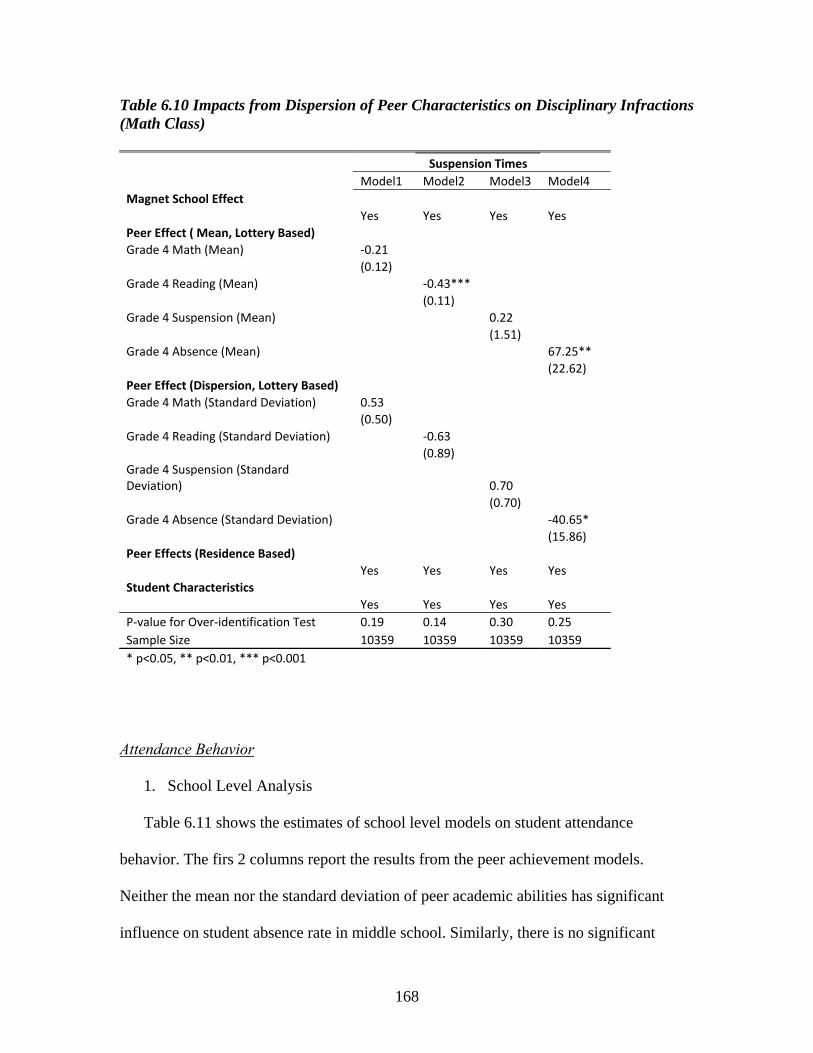
168

Table 6.10 Impacts from Dispersion of Peer Characteristics on Disciplinary Infractions (Math Class) Suspension Times



Yes Yes Yes Yes



(0.12)

Grade 4 Reading (Mean) ‐0.43***

(0.11)


(1.51)

Grade 4 Absence (Mean) 67.25**

(22.62)



(0.50)


(0.89) Grade 4 Suspension (Standard Deviation) 0.70

(0.70)

Grade 4 Absence (Standard Deviation) ‐40.65*

(15.86)


Yes Yes Yes Yes


Yes Yes Yes Yes


Sample Size 10359 10359 10359 10359

* p<0.05, ** p<0.01, *** p<0.001

Attendance Behavior


Table 6.11 shows the estimates of school level models on student attendance

behavior. The firs 2 columns report the results from the peer achievement models.

Neither the mean nor the standard deviation of peer academic abilities has significant

influence on student absence rate in middle school. Similarly, there is no significant

169

effect from either the mean or the standard deviation of peer prior disciplinary infractions

(Model 3). In model 4, the average peer absence rate and its standard deviation work in

opposite directions: while the average peer absence rate tends to raise the possibility of

absence, its standard deviation dispersion has a negative effect. Again, the much larger

and significant coefficient on the average peer absence rate is likely to be due to the high

collinearity between the average term and the variance term.

Table 6.11 Impacts from Variance of Peer Characteristics on Absence Rate (School Level) Absence Rate


Magnet School Effect Yes Yes Yes Yes Peer Effect ( Mean, Lottery Based)


(0.01)


(0.01)


(0.03)

Grade 4 Absence (Mean) 0.80*

(0.40)



(0.01)


(0.01)


(0.01)

Grade 4 Absence (Standard Deviation) ‐0.47**

(0.16)


Yes Yes Yes Yes


Yes Yes Yes Yes


Sample Size 12192 12192 12192 12192

* p<0.05, ** p<0.01, *** p<0.001

170


There is little evidence that changes in the heterogeneity of peer achievement or past

behavior at the classroom level affects student attendance behavior. The coefficients on

the average peer outcome variables remain insignificant, too. Although not shown in the

table, controlling for peer heterogeneity does not change the coefficients on other

variables: particularly, attending the academic magnet school appears to decrease student

absenteeism.

Table 6.12 Impacts from Variance of Peer Characteristics on Absence Rate (Math Class) Absence Rate Independent Variables Model1 Model2 Model3 Model4 Magnet School Effect Yes Yes Yes Yes Peer Effect ( Mean, Lottery Based) Grade 4 Math (Mean) 0.00 (0.00) Grade 4 Reading (Mean) 0.00 (0.00) Grade 4 Suspension (Mean) 0.07 (0.04) Grade 4 Absence (Mean) ‐0.07 (0.55) Peer Effect (Dispersion, Lottery Based) Grade 4 Math (Standard Deviation) ‐0.00 (0.01) Grade 4 Reading (Standard Deviation) ‐0.00 (0.02) Grade 4 Suspension (Standard Deviation) ‐0.02 (0.02) Grade 4 Absence (Standard Deviation) ‐0.23 (0.39) Peer Effects (Residence Based) Yes Yes Yes Yes Student Characteristics Yes Yes Yes Yes P‐value for Over‐identification Test 0.14 0.14 0.16 0.11 Sample Size 10359 10359 10359 10359 * p<0.05, ** p<0.01, *** p<0.001

171


This section examines whether peer group characteristics effects on student discipline

and attendance behaviors differ depending on individual background. The results in this

part answer the third research question --- to whom do peer effects matter more.



Many estimates of average school level peer effects are having unexpected coefficient

signs in previous Table 6.5. This part will find out if different subgroups of students are

impacted homogeneously by school level peer compositions. Regression results are

reported in Table 6.13, which includes coefficients on both the mean peer terms and the

interaction terms.

The first peer variable examined in this table is percent black students. Model 1

suggests that although other students are not significantly influenced by school black

population (even with a negative coefficient), black students tend to have more

suspensions while being in a school with disproportionately more Blacks. A similar

conclusion can be drawn from model 2, wherein the peer variable of percent black

students is found having a stronger and positive impact on students from low income

families. The linear combination of the coefficients on main effect and the interaction

with low SES variable is 0.9 (p<0.05), suggesting that low income students are likely to

receive 1 more suspension if they attend a school where the population is 100% Black

rather than 0% Black. Compared to boys, female students’ behaviors are less influenced

by black peers; and the influence from percent black students are stronger on low

172

achieving students than on high achieving students. However, the linear combinations of

the coefficients on the main effect and the interaction are not statistically significant.

Table 6.13 Heterogeneous Peer Effects on Disciplinary Infractions (School Level)

Suspension Times


Black LSES Female



Low Math achiever

High Math Achiever


Percent Black Students

Mean Effect ‐0.50 ‐0.12 0.48 0.09 0.13 0.03 0.08

(0.41) (0.37) (0.37) (0.36) (0.35) (0.36) (0.35)

Heterogeneous Effect 1.06*** 1.02*** ‐0.65*** 0.16* ‐0.01 0.20** 0.17

(0.22) (0.23) (0.16) (0.07) (0.11) (0.07) (0.11)


Mean Effect ‐1.35** ‐1.31** ‐0.56 ‐1.09* ‐1.03* ‐1.16** ‐1.09*

(0.44) (0.43) (0.44) (0.43) (0.43) (0.43) (0.43)

Heterogeneous Effect 1.02*** 1.12*** ‐0.67*** 0.19* ‐0.02 0.29** 0.19

(0.23) (0.31) (0.19) (0.09) (0.13) (0.09) (0.13)


Mean Effect 1.99*** 1.91*** 1.73*** 1.97*** 1.94*** 2.13*** 1.99***

(0.41) (0.41) (0.42) (0.41) (0.41) (0.42) (0.41)

Heterogeneous Effect ‐0.37*** ‐0.32*** 0.19* 0.02 0.20** ‐0.29** 0.21*

(0.10) (0.13) (0.08) (0.09) (0.07) (0.09) (0.07)


Mean Effect 1.42*** 1.39*** 1.19*** 1.41*** 1.38*** 1.51*** 1.41***

(0.36) (0.36) (0.36) (0.36) (0.36) (0.36) (0.36)

Heterogeneous Effect ‐0.43*** ‐0.41*** 0.20** 0.02 0.21** ‐0.32** 0.21**

(0.09) (0.11) (0.07) (0.08) (0.06) (0.08) (0.06)


Mean Effect ‐0.77 ‐0.49 ‐0.14 ‐0.36 ‐0.22 ‐0.71 ‐0.35

(0.53) (0.49) (20.55) (0.47) 0.47 (0.47) (0.48)

Heterogeneous Effect 1.19** 0.73 ‐0.11 0.31 ‐0.19 1.17*** 0.36

(0.47) (0.52) (0.44) (0.28) (0.40) (0.28) (0.39)

Peer Prior Absence Rate

Mean Effect ‐34.81** ‐32.61** ‐32.57** ‐35.18** ‐34.78** ‐35.20** ‐35.04**

(11.46) (11.17) (12.00) (11.12) (11.10) (11.11) (11.10)

Heterogeneous Effect 2.37 ‐7.79 ‐2.59 1.85 1.95 1.76 4.18**

(9.53) (10.46) (8.04) (1.19) (1.47) (1.18) (1.44)

* p<0.05, ** p<0.01, *** p<0.001

173

The second peer variable shown in this table is percent Low SES students. Recall that

in Table 6.5, school percent Low SES population reduces suspensions. The models in

Table 6.13 show that the negative association between percent low SES student variable

and student disciplinary infractions does not hold for every group of students. First, black

and low SES students appear to be not impacted by school low SES population: the

positive coefficients on the interaction term almost cancel out the negative coefficients on

the main effects in model 1 and model 2. Second, the negative impact of school percent

low SES students is not significant on male students. Third, although both high and low

achieving lottery participants seem to have fewer disciplinary infractions when there is a

high proportion of low SES students in the school, the negative impact is stronger on

students with higher prior test scores.

Both school level peer academic ability variables were found to increase student

disciplinary infractions in our sample. There are some significant heterogeneous effects

from both peer achievement variables. For example, the positive impact of peer

achievement is weaker on Blacks, low income students (model 1 and model 2), and low

performing students (model 6), but it is stronger on students with high prior achievement

(model 5 and model 7).

Average school peer prior disciplinary records do not have a significant impact on

student behaviors (as shown in Column9, Table 6.5). Although model 1 and model 6

show significant heterogeneous effect on Blacks and low math achievers, the linear

combination of the coefficients on the main effect and the interaction finds no evidence

that either of these groups is significantly influenced by peer prior disciplinary

infractions.

174

The last peer variable reported in Table 6.13 is peer prior attendance record, which is

negatively associated with individual disciplinary infractions for all groups of students.

The effect is slightly weaker on students with higher math scores.

Again, the estimates from the heterogeneous models on school level peer

characteristics support my previous hypothesis that advantaged students (e.g., students

from non-low-income families or high performing students) are less likely to receive

disciplinary actions if he is in a school with disproportional disadvantaged peers.


Table 6.14 presents the estimates of classroom level heterogeneous peer effect

models. As before, only results from math class peer variables are reported given that the

conclusions from peer variables in reading classes are very similar.

First, although high percentage of Black or low SES class peers tends to increase

individual misconduct for all students, the size of the impact is much stronger on Blacks,

students from low income families, and low achieving students. For example, combined

main effect and interaction for percent black students is 1.88 for low income students,

almost 3 times of the estimated effect (0.66) on students from affluent families. Girls are

less impacted by black or low SES peers than boys, although combined main effect and

interaction is still positive and significant for girls for both variables.

Second, average peer math achievement significantly reduces the number of

suspensions only for Blacks, boys, and low income students. However, the main effect of

peer reading achievement is significant and negative in all models. There is also

significant heterogeneity in this effect: Blacks and low income students appear to be

175

more negatively impacted by class average peer reading achievement; the negative

impact, however, is weaker on girls and students with high math scores.

Table 6.14 Heterogeneous Peer Effects on Disciplinary Infractions (Math Class) Suspension Times


Black LSES Female



Low Math achiever

High Math Achiever


Percent Black Students

Mean Effect 0.62** 0.66** 1.20*** 0.88*** 0.96*** 0.87*** 0.92***

(0.24) (0.22) (0.22) (0.22) (0.22) (0.22) (0.22) Heterogeneous Effect 0.81*** 1.22*** ‐0.49*** 0.23** ‐0.01 0.27*** 0.19

(0.19) (0.20) (0.14) (0.08) (0.14) (0.08) (0.13)


Mean Effect 0.79** 0.83*** 1.60*** 1.11*** 1.25*** 1.08*** 1.24***

(0.25) (0.25) (0.25) (0.24) (0.24) (0.24) (0.24) Heterogeneous Effect 1.29*** 1.43*** ‐0.71*** 0.34*** ‐0.10 0.36*** ‐0.03

(0.21) (0.25) (0.17) (0.10) (0.17) (0.10) (0.16)


Mean Effect ‐0.14 ‐0.13 ‐0.33* ‐0.18 ‐0.25 ‐0.19 ‐0.26

(0.13) (0.13) (0.13) (0.13) (0.13) (0.13) (0.13) Heterogeneous Effect ‐0.36*** ‐0.56*** 0.22** ‐0.17* 0.14* ‐0.13 0.11*

(0.13) (0.10) (0.07) (0.07) (0.06) (0.07) (0.06)


Mean Effect ‐0.30** ‐0.34** ‐0.52*** ‐0.38** ‐0.44*** ‐0.38** ‐0.45***

(0.12) (0.12) (0.12) (0.12) (0.11) (0.12) (0.11) Heterogeneous Effect ‐0.41*** ‐0.50*** 0.18** ‐0.13 0.11* ‐0.13* 0.11*

(0.08) (0.09) (0.06) (0.06) (0.06) (0.06) (0.05)


Mean Effect 0.55 1.42* 2.10*** 1.4** 1.76*** 1.34* 1.68***

(0.56) (0.62) (0.52) (0.52) (0.45) (0.53) (0.48) Heterogeneous Effect 2.35*** 0.66 ‐0.81 0.65 ‐0.11 0.89* 0.35

(0.58) (0.62) (0.52) (0.39) (0.87) (0.40) (0.73)


Mean Effect 6.77 29.31** 20.24* 27.75** 28.08** 27.64** 27.47**

(8.83) (9.69) (8.35) (9.54) (9.66) (9.54) (9.73) Heterogeneous Effect 76.70*** ‐4.40 16.61 3.22* 1.23 2.02 2.11

(14.81) (13.35) (11.06) (1.41) (1.80) (1.38) (1.73)

* p<0.05, ** p<0.01, *** p<0.001

176

Third, although the overall lottery participants seem to have more disciplinary

incidents if they are placed in a class with more misbehaving peers, two subgroups of

students seem to be impacted by peer disciplinary behaviors differently from other

students. A black student tends to receive 2.4 more suspensions if the average prior peer

suspensions increase by 1, while the coefficient on this variable is 0.55 and insignificant

for non-black students. Also, the effect is larger on students with low math achievement:

compared to other students, the students at the bottom quarter receive 1 more suspension

if the average prior peer suspensions increase by 1.

Finally, conclusions from the models of peer prior absence rates are very similar to

those from peer suspensions. The positive association between peer absence rate and

individual disciplinary infraction works mainly on black students, and the positive impact

is slightly larger on students with low reading achievement. Other models find no

significant heterogeneity in the effect of prior peer absences.

Attendance Behavior


Results for student attendance are presented in Table 6.15. Most peer characteristics

examined, including percent black students, percent low income students, average peer

math scores, average reading scores, and average prior absence rate, do not show a

significant influence on student attendance.

Interestingly, although Table 6.7 (column 9) suggests that average peer prior

disciplinary infractions increase student absence rate, the heterogeneous models find that

the estimated peer disciplinary record effect is not significant on every group of students.

177

For example, the attendances of black students, boys, and students in the middle quartiles

of achievement distributions are not significantly influenced by peer behavioral records,

but the linear combination test (see Appendix E) suggests that low income students, girls,

and low achievers are likely to be more absent if the school peers received more

suspensions in 4th grade.

Table 6.15 Heterogeneous Peer Effects on Absence Rate (School Level)

Absence Rate


Black LSES Female



Low Math achiever

High Math Achiever

Peer Effects (Lottery Based) Percent Black Students Mean Effect 0.00 0.00 0.00 ‐0.00 ‐0.00 ‐0.00 ‐0.00

(0.01) (0.01) (0.01) (0.01) (0.01) (0.01) (0.01) Heterogeneous Effect ‐0.01 ‐0.01 ‐0.01 0.00 0.01* ‐0.00 ‐0.00

(0.01) (0.01) (0.00) (0.00) (0.00) (0.00) (0.00) Percent Low SES Students Mean Effect 0.01 0.01 0.01 0.01 0.01 0.01 0.01

(0.01) (0.01) (0.01) (0.01) (0.01) (0.01) (0.01) Heterogeneous Effect ‐0.02* ‐0.01 0.01 0.01* 0.01* 0.00 ‐0.00

(0.01) (0.01) (0.01) (0.00) (0.00) (0.00) (0.00) Peer Prior Math Achievement Mean Effect ‐0.00 ‐0.00 ‐0.00 ‐0.00 ‐0.01 ‐0.00 ‐0.00

(0.01) (0.01) (0.01) (0.01) (0.01) (0.01) (0.01) Heterogeneous Effect 0.00 ‐0.00 ‐0.00 ‐0.00 0.00 ‐0.00 0.00

(0.00) (0.00) (0.00) (0.00) (0.00) (0.00) (0.00) Peer Prior Reading Achievement Mean Effect ‐0.01 ‐0.01 ‐0.01 ‐0.01 ‐0.01 ‐0.01 ‐0.01

(0.01) (0.01) (0.01) (0.01) (0.01) (0.01) (0.01) Heterogeneous Effect 0.00 ‐0.00 ‐0.00 ‐0.00 0.00 ‐0.00 0.00

(0.00) (0.00) (0.00) (0.00) (0.00) (0.00) (0.00) Peer Prior Disciplinary Records Mean Effect 0.04** 0.02 0.02 0.02 0.02 0.02 0.04**

(0.01) (0.01) (0.01) (0.01) (0.01) (0.01) (0.01) Heterogeneous Effect ‐0.02 0.03 0.01 0.01 0.02 0.01 ‐0.02

(0.01) (0.02) (0.01) (0.01) (0.01) (0.01) (0.01) Peer Prior Absence Rate Mean Effect 0.42 0.34 ‐0.07 0.30 0.31 0.32 0.32

(0.34) (0.33) (0.35) (0.33) (0.33) (0.33) (0.33) Heterogeneous Effect ‐0.44 ‐0.10 0.58* 0.05 0.10* ‐0.01 ‐0.01

(0.28) (0.31) (0.24) (0.04) (0.04) (0.03) (0.04)

* p<0.05, ** p<0.01, *** p<0.001

178


As shown in Table 6.16, the estimates of heterogeneous peer effect models on student

attendance behavior are quite simple: overall, most peer variables do not show significant

impacts on individual attendance; there are no significant heterogeneous effects in most

models either. Two exceptions are from average class prior absence rate. Non black

students and male students seem to be less absent when class absence rate is higher.

Again, neither the heterogeneous peer effect models nor the average peer effect

models (at both school and classroom levels) suggest that individual attendance behavior

change significantly in response to the changes in school or class peer composition.

Table 6.16 Heterogeneous Peer Effects on Absence Rate (Math Class) Absence Rate


Black LSES Female



Low Math Achiever

High Math Achiever

Peer Effects (Lottery Based) Percent Black Students

Mean Effect 0.00 0.00 0.01 0.00 0.00 0.00 0.00

(0.01) (0.01) (0.01) (0.01) (0.01) (0.01) (0.01) Heterogeneous Effect ‐0.00 ‐0.00 ‐0.01** 0.00 0.00 ‐0.00 0.00

(0.00) (0.00) (0.00) (0.00) (0.00) (0.00) (0.00) Percent Low SES Students

Mean Effect 0.01 0.00 0.01 0.00 0.01 0.01 0.01

(0.01) (0.01) (0.01) (0.01) (0.01) (0.01) (0.01) Heterogeneous Effect ‐0.00 0.00 ‐0.01 0.00 0.00 ‐0.01 0.00

(0.01) (0.01) (0.00) (0.00) (0.00) (0.00) (0.00) Peer Prior Math Achievement

Mean Effect 0.00 0.00 0.00 0.00 0.00 0.00 0.00

(0.00) (0.00) (0.00) (0.00) (0.00) (0.00) (0.00) Heterogeneous Effect 0.00 0.00 0.00 ‐0.00 0.004* 0.00 0.00


Mean Effect 0.00 0.00 0.00 0.00 ‐0.00 0.00 0.00

(0.00) (0.00) (0.00) (0.00) (0.00) (0.00) (0.00)

Heterogeneous Effect 0.00 ‐0.00 0.00 0.00 0.00 ‐0.00 0.00

(0.00) (0.00) (0.00) (0.00) (0.00) (0.00) (0.00) Peer Prior Disciplinary Records

Mean Effect 0.01 0.01 0.02 0.01 0.02 0.02 0.02

(0.01) (0.02) (0.01) (0.01) (0.01) (0.01) (0.01) Heterogeneous Effect 0.01 0.02 ‐0.00 0.02 0.01 0.00 ‐0.02

(0.01) (0.02) (0.01) (0.01) (0.02) (0.01) (0.02)

179

Table 6.16 Continued Peer Prior Absence Rate

Mean Effect ‐0.49* ‐0.24 ‐0.43* ‐0.34 ‐0.35 ‐0.32 ‐0.36

(0.21) (0.24) (0.21) (0.24) (0.24) (0.24) (0.24)


(0.36) (0.33) (0.28) (0.04) (0.04) (0.03) (0.04)

* p<0.05, ** p<0.01, *** p<0.001

Robustness Checks

Similar to the work on student academic achievement, I checked whether the

estimates of peer group effects on student behavioral outcomes are confounded with

heterogeneous treatment effects and teacher effects. There is no significant evidence that

the estimated peer effects on student discipline or attendance behaviors are confounded

heterogeneous treatment effects or teacher effects. In particular, with teacher fixed effects

in the model, the coefficients on class peer characteristics in the discipline outcome

models are even larger. Although including teacher fixed effect does not change the

estimated peer effects on student absence behavior, the academic magnet school

treatment effect became insignificant.

In addition, I also ran a set of school fixed effect models to see if the unexpected

coefficients on school level peer variables are impacted by some time-invariant school

factors (such as discipline policies). However, the conclusions regarding school level

peer characteristics remained unchanged.

180

CHAPTER VII

CONCLUSIONS

This dissertation investigates the peer group effects on student outcomes (both

academic and behavioral outcomes). Relying on the admission lotteries that randomly

assign students to a magnet school or a neighborhood school, this study implements

credible methods to identify peer effects free from selection bias and omitted variable

bias; it also circumvents the simultaneity bias by using lagged values of student

achievement and behavior records to form peer variables. The investigation of peer

effects answers three research questions:

What is the impact from average peer characteristics on individual

student outcomes at both school and classroom levels?

What is the impact of peer heterogeneity on student outcomes at both

levels?

To whom do peer effects matter the most? --- That is, which

subgroups of students are more impacted by peer characteristics?

This chapter will summarize the key findings, implications, and limitations of this study.

Review of Findings

Average Peer Effects

This study examines peer group effects from a large set of specifications of peer

characteristics at both school and classroom levels. Although both level analyses find

181

some large estimates of peer effects, there are many differences between the school level

estimates and the classroom estimates. The comparison of estimated peer effects at two

levels shows that the stronger peer influences come from classroom.

First, student achievement tends to be lower if they are surrounded by more black

peers at both school and classroom levels. The negative effect of percent black students

agrees with the findings from some recent literature, such as the Texas studies by Hoxby

(2004) and Hanushek, Kain, and Rivkin (2009). However, the two Texas studies also find

stronger intra-racial effects of average school percent black students. In this study, the

heterogeneous effect model does not suggest that black students are more negatively

impacted by school or classroom black population. One possibility is that the sample in

my study is limited to magnet school lottery participants. The black students in our

sample may be different from other black students in motivations and parental support,

and less susceptible to the influence of black peers.

Although school percent black students does not show significant impact on student

disciplinary behavior, classroom level analysis finds that having more black students in a

class increases disciplinary incidents. There is no evidence that school or classroom black

population influences individual attendance behavior in middle school.

Second, the effect of low income peers is not significant at the school level. The

school level finding agrees with previous studies by Hanushek et al (2003) and McEwan

(2004) which did not find significant impacts of percent low income students. However,

classroom level analysis found that percent low income student is associated with lower

academic achievement. The estimated effect at the classroom level is substantial: a 50%

182

change in classroom low income students leads to a 0.4 point decline in standardized

score changes in student math scores, and a 0.35 point decline in reading scores.

Third, although school level estimates of average peer achievement are not

significant, the average class peer achievement has a positive impact on student test

scores in both subjects. Because this study examines peer effects on middle school

students who are often grouped for classes based on academic abilities, it is likely that

average school level peer achievement has minimum impact on student outcomes.62 The

positive estimate of classroom peer achievement effect echoes the findings in some

literature, such as Betts and Zau (2004), and Lefgren (2007).

Interestingly, the school level analyses find that percent low SES students decreases

disciplinary problems in middle school and average peer achievement increases

individual disciplinary infractions. However, the estimated effects of the same peer

variables at the classroom level yield totally opposite conclusions: middle school

students are more likely to misbehave (measured by number of suspensions) if there are

more peers from low income families; and students tend to behave better if the classmates

have higher prior test scores (significant only for peer reading achievement). These

results suggest that the effects of peers are stronger and more direct at the classroom

level. The estimates of school level peer effects may well reflect how school student

composition impacts disciplinary actions (suspensions, as measured in this section).

Fourth, while classroom level prior peer disciplinary infractions significantly decrease

individual academic achievement and increase individual misconducts in middle school,

62 Both Hoxby (2001) and Hanushek et al (2000) found that school level average peer achievement improves student test scores. However, their studies focus on elementary school students. Given that there is often general teaching and few ability tracking, the mix of students in any class may just mirror the school as a whole in elementary schools.

183

the effect of peer disciplinary records at school level is not significant at all. This again

suggests that a stronger and more direct peer effect happens at the classroom level.

Finally, there is no evidence in our data that percent female students improves student

academic achievement or decreases disciplinary incidences; and average peer attendance

behavior does not show any significant impact on individual achievement or behavior at

either the school or classroom level.

Another important finding from the peer effect models is that adding peer

characteristics into the model totally overturn the significant treatment effect of the

academic magnet school in many models. In particular, when the average classroom peer

reading achievement is controlled, the estimate of academic magnet treatment effect on

student math achievement becomes significantly negative. This implies that lottery losers

who attend the neighborhood schools can do even better in academics than the academic

magnet enrollees if the classroom peers are the same. It also indicates that superior peer

composition makes a large contribution to the success of magnet programs.

Effects of peer heterogeneity

School level analyses find some significant effects of peer heterogeneity. The average

student test scores in both subjects tend to increase if the variation in prior peer reading

achievement is larger; and student disciplinary incidents decrease when the variation in

peer academic qualities is larger.

However, there is little evidence that changes in the heterogeneity of classroom peer

characteristics (prior peer achievement, disciplinary records, or attendance records)

impact student academic achievement or behavioral outcomes. The findings at the

184

classroom level do not suggest that within school ability grouping has a significant

influence on student outcomes.

Heterogeneous peer effects

The estimates of peer group effects are different on some students depending on their

demographic characteristics and academic abilities. First, although no evidence shows

that academic achievement of black or low income students decline with a high

proportion of peers from the same group, there is a strong intra-group impact on

individual disciplinary outcomes for Blacks and low income students at both the school

and classroom levels.

Second, the estimates of peer group effects are less strong on female students than on

male students. This is true of both academic achievement and disciplinary outcomes at

both the school and classroom levels.

Third, academically, both high and low performing students appear to be more

negatively impacted by percent black or low income students, but less positively

impacted by average peer academic achievement. However, a significant heterogeneous

effect on disciplinary outcomes is only found for low performing students, who are more

likely to receive suspensions if there is a high proportion of disadvantaged peers.

Finally, there is no significant heterogeneous peer effect on student attendance

outcomes, either with respect to mean peer characteristics or their variance within the

classroom.

185

Implications and Limitations

Research Implications

This dissertation yields its research implications on two fronts. First, this study adds

an empirical piece to the growing literature that implements credible strategies to identify

peer group effects on student outcomes. Second, the various methods used in this study to

deal with complications in randomized data have important implications for research with

experimental design.

Empirical studies on peer effects are plagued by the critical issues of selection bias

and simultaneity bias. This dissertation improves on previous attempts to eliminate self

selectivity by employing both randomization and instrument variable methods. In

specific, the identification strategies used in this study ensures the estimation of peer

effects free of selectivity by exploiting randomly determined lottery outcomes to

construct exogenous sources of variation in peer characteristics.

In recent years, two pieces of federal legislation the No Child Left Behind Act of 2001

(NCLB) and the Education Sciences Reform Act of 2002 (ESRA) have led to a rising

demand of experimental research using random assignment to produce more rigorous

evidences in evaluating education intervention programs. While randomization through

experiments is considered as the most promising method to obtain unbiased estimates of

causal effects, there are many complications in social experiments that may threat the

validity of the randomness, such as non-compliance, selective attrition, and

heterogeneous responses to treatment effects. This study presents detailed discussions of

the complications that arise in the magnet program admission lotteries. The solutions to

186

these complications adopted here contribute to the education research by offering

workable approaches to using these sorts of data to address policy questions.

Policy Implications

From the perspective of practice, this study also has important policy implications.

Although attending the academic magnet program in the district studied improves student

academic achievement in both math and reading, this effect can be entirely accounted for

by the peer characteristics. While this finding suggests that peer group characteristics

make a large contribution to the magnet school success, it also implies that district

administrators or policy makers need alternative assessment models while evaluating

schools and teachers based on student test scores. Student characteristics or peer

compositions should be incorporated in the models assessing teacher (school)

effectiveness, or schools and teachers will be held accountable for factors that are beyond

their control.

Second, scholars have argued that socioeconomic isolation of poor, minority students

in urban school systems is a major cause of the continuing achievement gap (see

Kahlenberg (2001) for a summary). Magnet program has been considered as an important

mechanism to reform urban districts through decreasing racial or social-economical

segregation as well as improving student achievement. However, this study finds that

students from magnet schools are mostly benefiting from superior peer groups. This

finding provides some evidences to the policy makers that magnet schools have not

actually reduced the socioeconomic isolation but may have exacerbated the within-

district inequality by creaming off good students from conventional schools.

187

Third, this study finds large and negative impact of average peer disciplinary

infractions on student outcomes (both academic and behavior), which indicates that

middle school students are very sensitive to the misconducts of their peers. Therefore, in

addition to the standard test scores of students, reduction of student misbehavior and

improvement of safe school environment should also be an important element in

assessing school effectiveness.

Finally, there is no evidence from either the school level or classroom level analyses

that change in the heterogeneity of peer composition influences student outcomes.

Moreover, the heterogeneous effect models do not find that any specific student group is

significantly impacted by the heterogeneity of peer characteristics. These findings

suggest that ability tracking per se has no impact on student achievement, at least not on

the lottery participants in the district studied.

Limitations

This study is limited in several respects. First, the investigation of peer effects in this

study relies on data from only one district. Compared to other studies using state-wide

data (such as the Texas studies by Hanushek et al. and Hoxby, and the North Carolina

study by Vigdor and Nechby etc), this study contains far less observations. Although the

district examined in this study is similar to other urban school systems in many ways,

how well these findings generalized is unknown.

Second, because the research design relies on lottery randomization to estimate peer

effects, the inferences are limited to a subset of students who participate in the lotteries.

This strategy excludes the large number of students who do not express an interest in

188

attending magnet schools, and the smaller number of students who are admitted in other

ways (e.g., through sibling preferences or neighborhood zone preferences). Similarly, the

conclusions about peer effects from this study can not be fully extended to students

unlike those participating in the lotteries.

Third, in order to circumvent the simultaneity bias, this project does not estimate the

endogenous peer effects --- contemporaneous peer achievement or behavioral measures.

Instead, the investigation of peer effects focuses on contextual effects, represented by

peer academic ability (measured by lagged academic outcomes) and other predetermined

peer characteristics. While endogenous peer effects imply potentially large social

multiplier effects and efficiency gains through the feedback in the behavior of individuals

within an existing social network (e.g., Hoxby argues that positive student behavior leads

to more positive behavior in the network), contextual peer effects do not have these

dynamic implications.

Finally, using lagged values of peer scores and behavioral records may not

completely remove the reflection problems due to the serial correlations between the

measurement errors in the lagged outcomes and those in current outcomes. However,

controlling for student prior outcomes in the data greatly reduces the correlation between

current outcomes and the measurement errors in lagged peer outcomes. Moreover, given

the facts that we use students’ 4th grade scores to construct peer academic ability

measures and most students in the district go to a new middle school after 4th grade, the

serial correlation are less likely to cause significant simultaneity bias in the estimation of

the effects from current peers.

189

Appendix A

Prediction of Peer Characteristics in Neighborhood Schools ( )NP

As introduced in Chapter III, although the admission lottery randomly assigns lottery

participants to a treatment group (a magnet school) or a control group (a neighborhood

school), neighborhood schools still vary across lottery participants. The neighborhood

school where a lottery participant is expected to attend if not admitted by a magnet school

reflects family residence choices, and is very likely to be related to unobserved factors

that also influence student outcomes. In order to eliminate the selection bias arising from

neighborhood choices, we include the variable NP as an independent variable in the

regression.

However, NP is not observable for students who are enrolled in the magnet schools.

Therefore, we need to predict the value of NP . The prediction of NP is based on the

sample of students who lost all middle school lotteries and attended regular public

schools in the district. The prediction model can be specified as:

iglNP , )( , igligl SXf (A.1)

where iglNP , is a set of neighborhood school peer variables for lottery loser i in grade g

and lottery year l (cohort indicator), iglX is a vector of lottery losers’ demographic

characteristics and prior achievements, iglS indicates the elementary school where lottery

loser i attended in 4th grade. As indicated by the model, the prediction models are run for

every grade and every lottery cohort separately. Although the regression is only limited to

190

the sample of lottery losers, the predicted value of NP̂ is assigned to all lottery

participants in the same grade and same cohort63. For example, if student A and student B

are from the same elementary school and share very similar demographic attributes (race,

gender, SES, special ed, and ELL) as well as 4th grade test scores, each of them is

assigned a predicted NP̂ with close values regardless of their lottery outcomes.

The following table provides some descriptive statistics of predicted counterfactual

neighborhood school peer variables ( NP̂ ) for 5th graders in two cohorts: lottery year 2000

and lottery year 2001. The second column (“Group”) indicates that students are from the

same 4th grade school, same ethnicity group and same social economic status group. As

we can see from the table, regardless of their lottery outcomes, the predicted value of

neighborhood school peer characteristics are very similar for students sharing same

attributes in race, SES and elementary schools.

Table A.1 Counterfactual School Peer Variables for 5th graders

Lottery Year Group

Lottery outcomes Obs

Predicted Neighborhood school Peer Variables

Black Low SES Grade 4 Math Grade 4 Reading

Pct SD Pct SD Mean SD Mean SD

2000 1 Win 11 33.1 2.7 11.4 1.9 0.67 0.06 0.82 0.07

Lose 13 32.9 2.4 11.1 1.7 0.67 0.07 0.84 0.08

2000 2 Win 18 28.5 1.5 18.1 2.5 0.44 0.04 0.61 0.05

Lose 7 28.9 1.4 19.1 2.2 0.42 0.04 0.58 0.05

2001 3 Win 20 31.6 1.9 30.0 2.3 0.42 0.02 0.42 0.02

Lose 13 32.7 2.3 31.7 3.2 0.43 0.03 0.44 0.03

2003 4 Win 25 31.3 7.6 31.3 5.5 0.16 0.03 0.30 0.03

Lose 8 30.6 4.4 31.0 4.4 0.15 0.01 0.29 0.02

Note: Lottery outcome 'WIN' means the student won at least one lottery;

'LOSE' means the student lost all lotteries.

63 In order to avoid introducing a difference between students whose NP is observed (lottery losers) and

students whose NP is a counterfactual prediction, the predicted NP̂ are used in all final models for all

students.

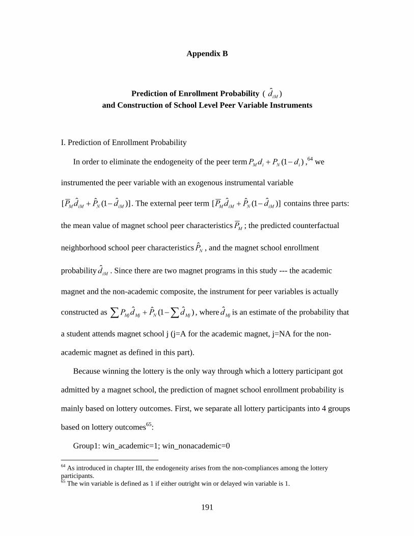
191

Appendix B

Prediction of Enrollment Probability ( )ˆiMd

and Construction of School Level Peer Variable Instruments

I. Prediction of Enrollment Probability

In order to eliminate the endogeneity of the peer term )1( iNiM dPdP ,64 we

instrumented the peer variable with an exogenous instrumental variable

)]ˆ1(ˆˆ[ iMNiMM dPdP . The external peer term )]ˆ1(ˆˆ[ iMNiMM dPdP contains three parts:

the mean value of magnet school peer characteristics MP ; the predicted counterfactual

neighborhood school peer characteristics NP̂ , and the magnet school enrollment

probability iMd̂ . Since there are two magnet programs in this study --- the academic

magnet and the non-academic composite, the instrument for peer variables is actually

constructed as )ˆ1(ˆˆ MjNMjMj dPdP , where Mjd̂ is an estimate of the probability that

a student attends magnet school j (j=A for the academic magnet, j=NA for the non-

academic magnet as defined in this part).

Because winning the lottery is the only way through which a lottery participant got

admitted by a magnet school, the prediction of magnet school enrollment probability is

mainly based on lottery outcomes. First, we separate all lottery participants into 4 groups

based on lottery outcomes65:

Group1: win_academic=1; win_nonacademic=0

64 As introduced in chapter III, the endogeneity arises from the non-compliances among the lottery participants. 65 The win variable is defined as 1 if either outright win or delayed win variable is 1.

192

Group2: win_academic=0, win_nonacademic=1



Accordingly, each student received 4 group indicators: group1=1 for students in the 1st

group, 0 otherwise, and till group4.

Second, we define 4 magnet school enrollment probability variables for every lottery

participants in the sample: 1AMd and 2AMd as the enrollment probabilities in the academic

magnet school; and 1NAMd and 2NAMd as the non-academic magnet composite enrollment

probabilities. The initial values of all four probability variables are set to be zero.

Third, we run the regression models to predict magnet school enrollment probabilities

for students in each group separately. In specific, the equations are:

For Group1 students:

iAM1 ),,,( iiii GLOLXf (B.1)


iAM 2 ),,,( iiii GLOLXf (B.2)


iNAM1 ),,,( iiii GLOLXf (B.3)


iNAM 2 ),,,( iiii GLOLXf (B.4)

where iAM1 is a dichotomous variable indicating whether student i from group 1 is

enrolled in the academic magnet school, iAM 2 for student i from group 3;

iNAM1 indicates the non-academic magnet enrollment from students from group 2,

193

iNAM 2 for students from group 3. Other variables included in the models are: iX is a

vector of individual characteristics; iL is a lottery indicator which combines the

information of lottery year and lottery application; iLO is the lottery outcome indicator

including outright win and delayed win for both magnet programs; and iG is a grade

indicator. The predicted value of the dependent variable in each model is then assigned to

every student to replace the initial zero value of the enrollment probability: 1ˆ

AMd = iMA 1ˆ ,

2ˆ

AMd = iMA 2ˆ ; 1ˆ

NAMd = iMAN 1ˆ , 2ˆ

NAMd = iMAN 2ˆ .

Based on the predicted magnet school enrollment probabilities, we also defined 4

variables representing the enrollment probabilities in non-magnet schools:

1ˆ1NMd 1

ˆAMd ; 1ˆ

2NMd 1ˆ

NAMd ; 1ˆ3NMd 2

ˆAMd - 2

ˆNAMd ; 1ˆ

4 NMd . Therefore, each

student in our sample has 4 group indicator variables, 4 magnet school enrollment

probability variables, and 4 non-magnet school enrollment probability variables. Finally,

the enrollment probabilities for the academic magnet school, the non-academic magnet

composite and non magnet schools are:

Academic Magnet School: 3*ˆ1*ˆˆ21 groupdgroupdd AMAMAM (B.5)

Non-academic Magnet School: 3*ˆ2*ˆˆ21 groupdgroupdd NAMNAMNAM (B.6)

Non Magnet School:

4*ˆ3*ˆ2*ˆ1*ˆˆ4321 groupdgroupdgroupdgroupdd NMNMNMNMNM (B.7)

The following Table B.2 presents the predicted enrollment probabilities for 5th grade

students in different groups across lottery years. The predicted values of enrollment

probabilities reveal similar messages as shown in Table 3.3 (magnet school lotteries and

5th grade enrollment) in Chapter III: there is a high non-compliance rate among lottery

194

participants of the non-academic magnet composite; most students who won both

lotteries chose to attend the academic magnet.

Table B.2 Enrollment Probability by lottery outcome Groups (5th Grade)

Enrollment Probability

Lottery Year Group Academic Non‐Academic Non Magnet

Mean SD Mean SD Mean SD

1999 1 0.77 0.09 0.00 0.00 0.23 0.09

2 0.00 0.00 0.54 0.08 0.46 0.08

3 0.74 0.20 0.04 0.12 0.22 0.13

4 0.00 0.00 0.00 0.00 1.00 0.00

2000 1 0.76 0.12 0.00 0.00 0.24 0.12

2 0.00 0.00 0.59 0.08 0.41 0.08

3 0.68 0.13 0.07 0.05 0.26 0.10

4 0.00 0.00 0.00 0.00 1.00 0.00

2001 1 0.82 0.09 0.00 0.00 0.17 0.09

2 0.00 0.00 0.57 0.07 0.43 0.07

3 0.71 0.16 0.16 0.12 0.13 0.09

4 0.00 0.00 0.00 0.00 1.00 0.00

2002 1 0.87 0.07 0.00 0.00 0.13 0.07

2 0.00 0.00 0.64 0.08 0.36 0.08

3 0.84 0.12 0.06 0.06 0.11 0.08

4 0.00 0.00 0.00 0.00 1.00 0.00

2003 1 0.86 0.07 0.00 0.00 0.14 0.07

2 0.00 0.00 0.66 0.08 0.34 0.08

3 0.70 0.16 0.10 0.13 0.20 0.09

4 0.00 0.00 0.00 0.00 1.00 0.00

Note: Group1 students only won the academic magnet lottery;

Group2 students only won the non‐academic lottery;

Group3 won both lotteries; Group4 students lost both lotteries

II. Construction of School Level Peer Variable Instrument

After predicting the enrollment probability, the next step is to construct the

instrumental variable )ˆ1(ˆˆ MjNMjMj dPdP , or .ˆˆˆNMNMjMj dPdP In specific, the

instrumental variable for peer characteristics is constructed as:

195

)ˆ1(ˆˆ MjNMjMj dPdP =

)4*ˆ3*ˆ2*ˆ1*ˆ(*ˆ

)3*ˆ2*ˆ(*)3*ˆ1*ˆ(*

4321

2121

groupdgroupdgroupdgroupdP

groupdgroupdPgroupdgroupdP

iNMiNMiNMiNMN

iNAMiNAMNAMiAMiAMAM

(B.8)

where AMP is the mean value of school peer variable in the academic magnet school,

NAMP represents mean school peer variable in the non-academic composite, and NP̂ is the

predicted neighborhood school peer characteristics.

Note that there are 4 schools in the non-academic magnet composite. Therefore, the

values of NAMP is a weighted mean of the average peer characteristics in each non-

academic magnet school, wherein the weight is the fraction of numbers of outright

winner in each school over the total numbers of outright winners in the composite:

NAMP = jNAMjNAMj

winnersoutrightNoP _.(*4

1

)_.4

1jNAM

j

winnersoutrightNo

(B.9)

196

Appendix C

Construction of Instruments for Classroom Level Peer Variables

In order to eliminate the endogeneity of the classroom peer variable cijP , we

instrumented this variable using the model

iiiMcNiMcMcij XdPdPP )]ˆ1(ˆˆˆ[ (1st stage IV model)

where )ˆ1(ˆˆˆiMcNiMcM dPdP serves as the external instrumental variable. There are three

components in this instrumental variable: iMd̂ is an prediction of the probability that

student i attend the magnet school; cMP̂ is the predicted classroom peer variable in magnet

schools, which serves as the counterfactual class peers that lottery losers would encounter

in classes if they had won the magnet school lottery; cNP̂ is the predicted classroom peer

variable in neighborhood schools, which serves as the counterfactual class peers that

lottery winners would encounter in classes if they had lost the magnet school lottery and

enrolled in a neighborhood school.

Since the prediction of the first component iMd̂ has been introduced in Appendix B,

this part will focus on explaining the procedures predicting cMP̂ and cNP̂ . The prediction of

cMP̂ is done separately for each magnet school (the academic magnet and the four non-

academic magnet schools) by cohort and by grade --- for example, the models that predict

class peer characteristics in the academic magnet school cAMP̂ are only limited to a sample

of students enrolling in this academic magnet school. Moreover, because students in

197

middle schools are often grouped for instructions based on their academic ability (or

possibly based on behavioral problem), the prediction models include all individual

demographic variables as well as prior outcomes (academic and behavior outcomes); the

prediction also controls for a set of student 4th grade school indictors given that student

elementary school may carry some unobserved information influencing both outcomes

and class assignments in middle school. The prediction model for cMP can be expressed as

the following:

),(, igligliglcjM SXfP (C.1)

where iglcjMP

,indicates the classroom peer characteristics in magnet school j for student i

in grade g and lottery year (cohort) l, iglX is a vector of individual demographic variables

and prior outcomes, and iglS represents 4th grade school indicators. Although the

prediction of cjMP is only limited to students enrolled in magnet school j, the predicted

value is assigned to every student in the same grade and cohort regardless of the lottery

status and enrollment status. Similarly, the predicted classroom peer characteristics in the

non-academic magnet composite is a weighted mean of the class peer variables in all

non-academic magnet schools

cNAMP̂ = jNAMcjNAMj

winnersoutrightNoP _.(*ˆ4

1

)_.4

1jNAM

j

winnersoutrightNo

(C.2)+

The prediction of classroom peer characteristics in the neighborhood schools cNP̂

focuses on the sample of lottery losers. Different from models predicting cjMP , the

prediction of cNP is conducted within each elementary school, so that there are more

198

heterogeneous class assignments for students from the same elementary school. In

specific, the prediction model is:

)(, igsligslcN XfP (C.3)

where igslcNP , is the classroom peer characteristics for lottery loser i (who is from

elementary school s in 4th grade) in grade g and lottery year l , and igslX is a set of

individual factors. After each prediction, the predicted value of cNP̂ is assigned to both

lottery winners and lottery losers in the same grade and cohort.

Each student in our sample is assigned both predicted values of cMP̂ and cNP̂ , which

are incorporated with the enrollment probabilities to construct instrumental variables for

the true classroom peer characteristics:

)ˆ1(ˆˆˆiMcNiMcM dPdP =

)4*ˆ3*ˆ2*ˆ1*ˆ(*ˆ

)3*ˆ2*ˆ(*ˆ)3*ˆ1*ˆ(*ˆ

4321

2121

groupdgroupdgroupdgroupdP

groupdgroupdPgroupdgroupdP

iNMiNMiNMiNMicN

iNAMiNAMNAMiciAMiAMAMic

(C.4)

As Table 3.4 in chapter III already shows, the instrumental variables for classroom peer

characteristics are very close to the true values of classroom peer variables.

199

Appendix D

Validity of the Instrumental Variables

A valid instrumental variable has to meet two requirements: first, the IV must be

orthogonal to the error term; second, the IV must be correlated to the endogenous

regressor of interest. All peer effect models in this study include two sets of external

instruments: lottery outcomes ( ), 21 ii rr as instruments for the magnet school treatment

effect id ; )ˆ1(ˆˆiMNiMM dPdP as the instruments for school level peer characteristics, or

)ˆ1(ˆˆˆiMcNiMcM dPdP as the instruments for classroom level peer characteristics.

The omnibus over-identification tests of all regression models in Chapter IV to

Chapter VI (As shown at the bottom of the result tables) have provided strong evidence

that both sets of external instruments are orthogonal to the error terms and meet the first

validity requirement of exogeneity. Therefore, in this part, I will examine whether the

instruments meet the second validity requirement: correlated with the regressors of

interest.

As introduced in Chapter II, the estimates of peer effect are yielded from a 2 Stage

Lease Square (2SLS), wherein the first level model predicts the endogenous peer

variables from the instrumental variables. Therefore, the coefficients on the instrumental

variables from the first stage regression represent the correlation between the instruments

and the regressors of interest.

Table D.1 presents the estimates of first stage models of school level peer effects on

math achievement (the single variable models in Table 4.6 in Chapter IV). There are 10

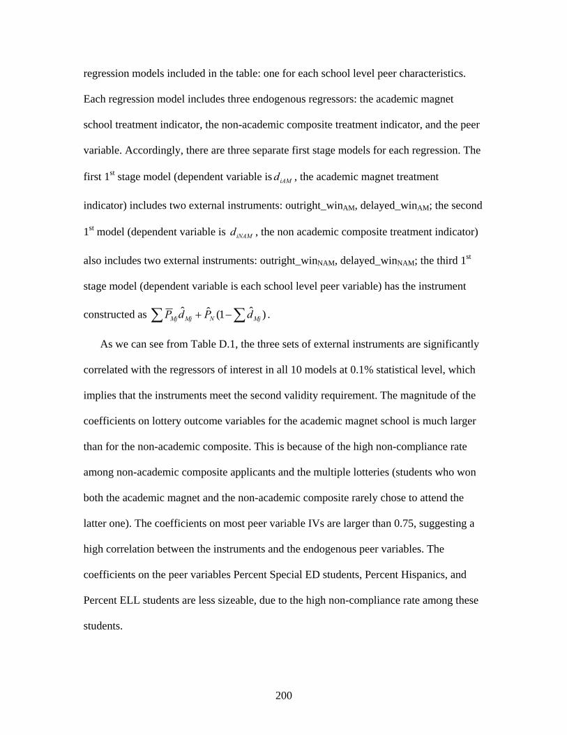
200

regression models included in the table: one for each school level peer characteristics.

Each regression model includes three endogenous regressors: the academic magnet

school treatment indicator, the non-academic composite treatment indicator, and the peer

variable. Accordingly, there are three separate first stage models for each regression. The

first 1st stage model (dependent variable is iAMd , the academic magnet treatment

indicator) includes two external instruments: outright_winAM, delayed_winAM; the second

1st model (dependent variable is iNAMd , the non academic composite treatment indicator)

also includes two external instruments: outright_winNAM, delayed_winNAM; the third 1st

stage model (dependent variable is each school level peer variable) has the instrument

constructed as )ˆ1(ˆˆ MjNMjMj dPdP .

As we can see from Table D.1, the three sets of external instruments are significantly

correlated with the regressors of interest in all 10 models at 0.1% statistical level, which

implies that the instruments meet the second validity requirement. The magnitude of the

coefficients on lottery outcome variables for the academic magnet school is much larger

than for the non-academic composite. This is because of the high non-compliance rate

among non-academic composite applicants and the multiple lotteries (students who won

both the academic magnet and the non-academic composite rarely chose to attend the

latter one). The coefficients on most peer variable IVs are larger than 0.75, suggesting a

high correlation between the instruments and the endogenous peer variables. The

coefficients on the peer variables Percent Special ED students, Percent Hispanics, and

Percent ELL students are less sizeable, due to the high non-compliance rate among these

students.

201

Table D.1 First Stage Regression (School Level): Correlations between Endogenous Regressors and the Instrumental Variables Model1 Model2 Model3 Model4 Model5 Model6 Model7 Model8 Model9 Model10

Magnet School Treatment Indicators

Academic Magnet

Outright Win 0.67*** 0.62*** 0.73*** 0.73*** 0.76*** 0.76*** 0.53*** 0.54*** 0.74*** 0.73***

(0.01) (0.01) (0.01) (0.01) (0.01) (0.01) (0.01) (0.01) (0.01) (0.01)

Delayed Win 0.57*** 0.53*** 0.63*** 0.62*** 0.65*** 0.65*** 0.46*** 0.46*** 0.63*** 0.62***

(0.01) (0.01) (0.01) (0.01) (0.01) (0.01) (0.01) (0.01) (0.01) (0.01)

Non‐Academic Composite

Outright Win 0.27*** 0.29*** 0.25*** 0.28*** 0.29*** 0.29*** 0.29*** 0.29*** 0.29*** 0.26***

(0.01) (0.01) (0.01) (0.01) (0.01) (0.01) (0.01) (0.01) (0.01) (0.01)

Delayed Win 0.24*** 0.26*** 0.22*** 0.25*** 0.26*** 0.27*** 0.26*** 0.26*** 0.26*** 0.23***

(0.01) (0.01) (0.01) (0.01) (0.01) (0.01) (0.01) (0.01) (0.01) (0.01)

Peer Variables

Black (Proportion)

Black IV 0.80***

(0.02)

Low SES (Proportion)

Low SES IV 0.81***

(0.02)

Female (Proportion)

Female IV 0.78***

(0.02)

Special ED (Proportion)

Special ED IV 0.29***

(0.02)

Hispanic (Proportion)

Hispanic IV 0.42***

(0.02)

ELL (Proportion)

ELL IV 0.19***

(0.01)

Mean G4 Math

Mean G4 Math IV 0.67***

(0.03)

Mean G4 Reading

Mean G4 Reading IV 0.69***

(0.01)

Mean G4 Suspension

Mean G4 Suspension IV 0.94***

(0.03)

Mean G4 Absence

Mean G4Absence IV 0.76***

(0.03)

202

Table D.2 reports the estimates of first stage models of classroom level peer effects

on math achievement (the single variable models in Table 5.1 in Chapter V). The

coefficients on the lottery outcomes for both magnet programs are very similar to the

estimates from school level models in last Table D.1, suggesting that the instruments and

the endogenous magnet school treatment variables are highly correlated. Although the

estimates of the classroom peer variable IVs are less sizeable than those from school level

models, the coefficients from all 10 models are significant at 0.1% statistical level. The

results again prove that the external instruments in our classroom level peer effect models

meet the second validity requirement of high correlation with the regressors.

Table D.2 First Stage Regression (Classroom Level): Correlations between Endogenous Regressors and the Instrumental Variables Model1 Model2 Model3 Model4 Model5 Model6 Model7 Model8 Model9 Model10

Magnet School Treatment Indicators

Academic Magnet

Outright Win 0.76*** 0.75*** 0.77*** 0.77*** 0.77*** 0.77*** 0.76*** 0.74*** 0.77*** 0.77***

(0.01) (0.01) (0.01) (0.01) (0.01) (0.01) (0.01) (0.01) (0.01) (0.01)

Delayed Win 0.68*** 0.67*** 0.69*** 0.69*** 0.69*** 0.69*** 0.67*** 0.66*** 0.69*** 0.69***

(0.01) (0.01) (0.01) (0.01) (0.01) (0.01) (0.01) (0.01) (0.01) (0.01)

Non‐Academic Composite

Outright Win 0.29*** 0.29*** 0.29*** 0.30*** 0.29*** 0.30*** 0.29*** 0.29*** 0.29*** 0.29***

(0.01) (0.01) (0.01) (0.01) (0.01) (0.01) (0.01) (0.01) (0.01) (0.01)

Delayed Win 0.27*** 0.28*** 0.28*** 0.28*** 0.28*** 0.28*** 0.28*** 0.27*** 0.28*** 0.27***

(0.01) (0.01) (0.01) (0.01) (0.01) (0.01) (0.01) (0.01) (0.01) (0.01)

Peer Variables

Black (Proportion)

Black IV 0.56***

(0.01)

Low SES (Proportion)

Low SES IV 0.54***

(0.01)

Female (Proportion)

Female IV 0.34***

(0.01)

Special ED (Proportion)

Special ED IV 0.23***

(0.02)

203

Table D.2 (Continued)

Hispanic (Proportion)

Hispanic IV 0.15***

(0.02)

ELL (Proportion)

ELL IV 0.12***

(0.01)

Mean G4 Math

Mean G4 Math IV 0.42***

(0.01)

Mean G4 Reading

Mean G4 Reading IV 0.56***

(0.02)

Mean G4 Suspension

Mean G4 Suspension IV 0.28***

(0.01)

Mean G4 Absence

Mean G4Absence IV 0.24***

(0.01)

In conclusion, the results from both the over-identification tests and the 1st stage

models suggest that the three sets of external instrumental variables in our peer effect

models are valid: they are exogenous to the error terms; and they are correlated with the

endogenous regressors.

204

Appendix E

Linear Combination Results of Heterogeneous Peer Effects

Both school level and classroom level analyses find that some students are impacted

by their peers more strongly than other students. The tables in Chapter IV (Table 4.10

and Table 4.11) and Chapter V (Table 5.5 and Table 5.6) present the estimates of

heterogeneous effects for seven different student groups. This part will report the

coefficients on peer variables from the linear combination tests, which shows the

estimates of peer effects on different students depending on their own background.

Since I have discussed many of the linear combination test coefficients in Chapter IV

to Chapter VI, this part will only reports the results.

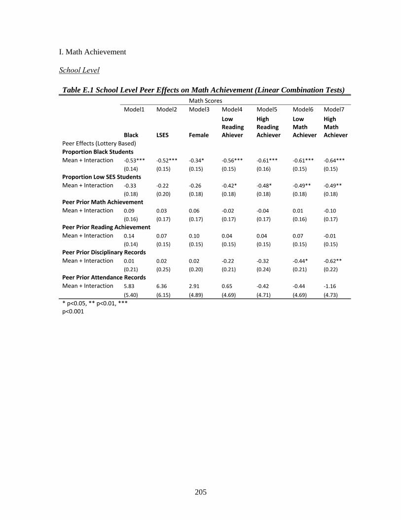
205

I. Math Achievement

School Level

Table E.1 School Level Peer Effects on Math Achievement (Linear Combination Tests) Math Scores


Black LSES Female

Low Reading Ahiever


Low Math Achiever

High Math Achiever


Proportion Black Students Mean + Interaction ‐0.53*** ‐0.52*** ‐0.34* ‐0.56*** ‐0.61*** ‐0.61*** ‐0.64***

(0.14) (0.15) (0.15) (0.15) (0.16) (0.15) (0.15)

Proportion Low SES Students

Mean + Interaction ‐0.33 ‐0.22 ‐0.26 ‐0.42* ‐0.48* ‐0.49** ‐0.49**

(0.18) (0.20) (0.18) (0.18) (0.18) (0.18) (0.18)


Mean + Interaction 0.09 0.03 0.06 ‐0.02 ‐0.04 0.01 ‐0.10

(0.16) (0.17) (0.17) (0.17) (0.17) (0.16) (0.17)


Mean + Interaction 0.14 0.07 0.10 0.04 0.04 0.07 ‐0.01

(0.14) (0.15) (0.15) (0.15) (0.15) (0.15) (0.15)


Mean + Interaction 0.01 0.02 0.02 ‐0.22 ‐0.32 ‐0.44* ‐0.62**

(0.21) (0.25) (0.20) (0.21) (0.24) (0.21) (0.22)


Mean + Interaction 5.83 6.36 2.91 0.65 ‐0.42 ‐0.44 ‐1.16

(5.40) (6.15) (4.89) (4.69) (4.71) (4.69) (4.73)

* p<0.05, ** p<0.01, *** p<0.001

206

Classroom Level

Table E.2 Heterogeneous Class Level Peer Effects on Math Achievement (Linear Combination Tests) (Math Class) Math Scores


Black LSES Female



Low Math Achiever

High Math Achiever


Proportion Black Students Mean + Interaction ‐0.63*** ‐0.59*** ‐0.58*** ‐0.71*** ‐0.76*** ‐0.78*** ‐0.83***

(0.10) (0.11) (0.10) (0.09) (0.10) (0.09) (0.10)


Mean + Interaction ‐0.81*** ‐0.73*** ‐0.69*** ‐0.86*** ‐0.94*** ‐0.93*** ‐0.91***

(0.11) (0.13) (0.11) (0.10) (0.11) (0.10) (0.11)


Mean + Interaction 0.37*** 0.35*** 0.29*** 0.30*** 0.25*** 0.29*** 0.25***

(0.06) (0.07) (0.06) (0.06) (0.06) (0.06) (0.06)



(0.05) (0.06) (0.05) (0.05) (0.05) (0.05) (0.05)


Mean + Interaction ‐0.44 ‐0.58** ‐0.60** ‐0.77*** ‐0.71 ‐0.92*** ‐0.77*

(0.23) (0.21) (0.23) (0.21) (0.40) (0.20) (0.32)


Mean + Interaction ‐5.08 ‐0.57 ‐5.49 ‐8.53* ‐8.77* ‐8.99* ‐8.43*

(7.28) (6.32) (5.65) (4.18) (3.94) (4.10) (3.99)

* p<0.05, ** p<0.01, *** p<0.001

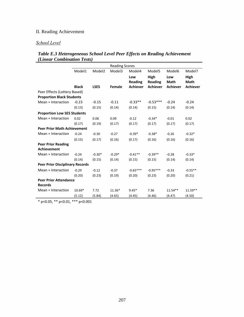
207

II. Reading Achievement

School Level

Table E.3 Heterogeneous School Level Peer Effects on Reading Achievement (Linear Combination Tests) Reading Scores


Black LSES Female



Low Math Achiever

High Math Achiever


Proportion Black Students Mean + Interaction ‐0.23 ‐0.15 ‐0.11 ‐0.33** ‐0.53*** ‐0.24 ‐0.24

(0.13) (0.15) (0.14) (0.14) (0.15) (0.14) (0.14)


Mean + Interaction 0.02 0.06 0.09 ‐0.12 ‐0.34* ‐0.01 0.02

(0.17) (0.19) (0.17) (0.17) (0.17) (0.17) (0.17)


Mean + Interaction ‐0.24 ‐0.30 ‐0.27 ‐0.39* ‐0.38* ‐0.26 ‐0.32*

(0.15) (0.17) (0.16) (0.17) (0.16) (0.16) (0.16)


Mean + Interaction ‐0.24 ‐0.30* ‐0.29* ‐0.41** ‐0.39** ‐0.28 ‐0.33*

(0.14) (0.15) (0.14) (0.15) (0.15) (0.14) (0.14)


Mean + Interaction ‐0.29 ‐0.12 ‐0.37 ‐0.65*** ‐0.95*** ‐0.33 ‐0.55**

(0.20) (0.23) (0.19) (0.20) (0.23) (0.20) (0.21)


Mean + Interaction 10.69* 7.72 11.36* 9.45* 7.36 11.54** 11.59**

(5.12) (5.84) (4.65) (4.45) (4.46) (4.47) (4.50)

* p<0.05, ** p<0.01, *** p<0.001

208

Classroom Level

Table E.4 Heterogeneous Class Level Peer Effects on Reading Achievement (Linear Combination Tests) (Reading Class) Reading Scores


Black LSES Female



Low Math Achiever

High Math Achiever


Proportion Black Students Mean + Interaction ‐0.50*** ‐0.49*** ‐0.39*** ‐0.62*** ‐0.83*** ‐0.54*** ‐0.51***

(0.10) (0.11) (0.10) (0.10) (0.10) (0.09) (0.10)


Mean + Interaction ‐0.74*** ‐0.71*** ‐0.54*** ‐0.85*** ‐1.07*** ‐0.76*** ‐0.63***

(0.11) (0.12) (0.11) (0.10) (0.11) (0.10) (0.11)


Mean + Interaction 0.28*** 0.25*** 0.20** 0.17** 0.10 0.24** 0.20**

(0.07) (0.08) (0.07) (0.07) (0.08) (0.07) (0.08)



(0.05) (0.05) (0.05) (0.05) (0.06) (0.05) (0.05)


Mean + Interaction ‐1.22*** ‐0.96*** ‐0.81*** ‐1.36*** ‐1.61*** ‐1.05*** ‐0.85**

(0.20) (0.19) (0.21) (0.17) (0.33) (0.17) (0.28)


Mean + Interaction ‐1.50 ‐5.39 3.71 ‐3.21 ‐4.57 ‐1.16 ‐0.69

(9.78) (9.04) (8.44) (6.05) (5.83) (5.99) (5.88)

* p<0.05, ** p<0.01, *** p<0.001

209

III. Disciplinary Infractions

School Level

Table E.5 Heterogeneous School Level Peer Effects on Disciplinary Infractions (Linear Combination Tests) Suspension Times


Black LSES Female



Low Math Achiever

High Math Achiever


Proportion Black Students Mean + Interaction 0.56 0.90* ‐0.17 0.25 0.12 0.24 0.26

(0.34) (0.36) (0.36) (0.35) (0.36) (0.35) (0.36)


Mean + Interaction ‐0.33 ‐0.19 ‐1.23** ‐0.91* ‐1.05* ‐0.87* ‐0.90*

(0.43) (0.48) (0.43) (0.43) (0.43) (0.43) (0.43)



(0.40) (0.43) (0.41) (0.43) (0.43) (0.41) (0.42)



(0.35) (0.37) (0.36) (0.38) (0.38) (0.36) (0.36)


Mean + Interaction 0.42 0.24 ‐0.25 ‐0.05 ‐0.42 0.46 0.01

(0.50) (0.57) (0.48) (0.50) (0.57) (0.49) (0.52)


Mean + Interaction ‐32.44* ‐40.50** ‐35.17** ‐33.33** ‐32.83** ‐33.45** ‐30.85**

(12.81) (14.22) (11.55) (11.08) (11.13) (11.11) (11.19)

* p<0.05, ** p<0.01, *** p<0.001

210

Classroom Level

Table E.6 Heterogeneous Class Level Peer Effects on Disciplinary Infractions (Linear Combination Tests) (Math Class) Suspension Times


Black LSES Female



Low Math Achiever

High Math Achiever


Proportion Black Students Mean + Interaction 1.43*** 1.88*** 0.71** 1.11*** 0.95*** 1.15*** 1.11***

(0.23) (0.26) (0.23) (0.21) (0.24) (0.22) (0.23)



(0.27) (0.29) (0.26) (0.24) (0.27) (0.24) (0.26)


Mean + Interaction ‐0.50** ‐0.69*** ‐0.12 ‐0.35** ‐0.11 ‐0.32* ‐0.14

(0.14) (0.15) (0.13) (0.13) (0.14) (0.13) (0.14)


Mean + Interaction ‐0.72*** ‐0.84*** ‐0.38** ‐0.51*** ‐0.33* ‐0.51*** ‐0.33**

(0.12) (0.13) (0.12) (0.12) (0.13) (0.12) (0.13)


Mean + Interaction 2.90*** 2.09*** 1.28* 2.10*** 1.65 2.23*** 2.03**

(0.53) (0.48) (0.53) (0.46) (0.95) (0.45) (0.75)


Mean + Interaction 83.47*** 24.91 36.84** 30.97** 29.31** 29.66** 29.57**

(17.71) (14.69) (13.43) (9.86) (9.31) (9.71) (9.43)

* p<0.05, ** p<0.01, *** p<0.001

211

IV. Attendance Behavior

School Level

Table E.7 Heterogeneous School Level Peer Effects on Attendance Behavior (Linear Combination Tests) Absence Rate


Black LSES Female



Low Math Achiever

High Math Achiever


Proportion Black Students Mean + Interaction ‐0.00 ‐0.01 ‐0.00 0.00 0.00 ‐0.00 ‐0.00

(0.01) (0.01) (0.01) (0.01) (0.01) (0.01) (0.01)


Mean + Interaction ‐0.00 0.00 0.01 0.01 0.02 0.01 0.01

(0.01) (0.01) (0.01) (0.01) (0.01) (0.01) (0.01)


Mean + Interaction ‐0.00 ‐0.00 ‐0.00 ‐0.01 ‐0.01 ‐0.01 ‐0.01

(0.01) (0.01) (0.01) (0.01) (0.01) (0.01) (0.01)



(0.01) (0.01) (0.01) (0.01) (0.01) (0.01) (0.01)


Mean + Interaction 0.02 0.04** 0.03* 0.04** 0.05** 0.03* 0.01

(0.01) (0.02) (0.01) (0.01) (0.02) (0.01) (0.01)


Mean + Interaction ‐0.02 0.24 0.50 0.35 0.41 0.31 0.30

(0.37) (0.42) (0.34) (0.33) (0.33) (0.33) (0.33)

* p<0.05, ** p<0.01, *** p<0.001

212

Classroom Level

Table E.8 Heterogeneous Class Level Peer Effects on Attendance Behavior (Linear Combination Tests) (Math Class) Absence Rate


Black LSES Female



Low Math Achiever

High Math Achiever


Proportion Black Students Mean + Interaction 0.00 0.00 ‐0.00 0.00 0.01 0.00 0.01

(0.01) (0.01) (0.01) (0.01) (0.01) (0.01) (0.01)


Mean + Interaction 0.00 0.01 0.00 0.01 0.01 0.00 0.01

(0.01) (0.01) (0.01) (0.01) (0.01) (0.01) (0.01)


Mean + Interaction 0.00 0.00 0.00 0.00 0.01 0.00 0.00

(0.00) (0.00) (0.00) (0.00) (0.00) (0.00) (0.00)


Mean + Interaction 0.00 ‐0.00 0.00 0.00 0.00 0.00 0.00

(0.00) (0.00) (0.00) (0.00) (0.00) (0.00) (0.00)


Mean + Interaction 0.02 0.03* 0.02 0.03* 0.02 0.02 0.00

(0.01) (0.01) (0.01) (0.01) (0.02) (0.01) (0.02)



(0.42) (0.36) (0.33) (0.25) (0.23) (0.24) (0.24)

* p<0.05, ** p<0.01, *** p<0.001

213

Appendix F

Reading Classroom Peer Effects on Behavioral Outcomes

Chapter VI reports and discusses the estimates of math class peer effects on student

disciplinary infractions and attendance rates. This part presents the regression results of

reading class peer effects on student behavioral outcomes. As usual, estimates of peer

effects from all three parts (the average peer effects, the effects from dispersion of peer

variables, and the heterogeneous peer effects) are reported in order. Although there are

some differences in the magnitudes of the coefficients on some peer variables between

math class estimates and reading class estimates, the overall conclusions are very similar.

Therefore, I am not going to discuss the results again in this part since Chapter VI has

provided detailed discussions.

214

I. Average Peer Effects


Table F.1 Average Classroom Peer Effects on Disciplinary Infractions (Reading Class) Suspension Numbers



Academic ‐0.11 0.00 ‐0.24** ‐0.32** ‐0.21* ‐0.24 ‐0.09 0.16 ‐0.20* 0.05 0.47*

(0.08) (0.11) (0.09) (0.10) (0.10) (0.15) (0.16) (0.13) (0.08) (0.15) (0.23) Non‐Academic Composite ‐0.34 ‐0.25 ‐0.33 ‐0.40 ‐0.33 ‐0.35 ‐0.31 ‐0.22 ‐0.33 0.06 0.27

(0.20) (0.20) (0.20) (0.21) (0.21) (0.22) (0.21) (0.21) (0.20) (0.27) (0.31)

Peer Effect (Lottery Based) Black (proportion) 0.82*** 0.84

(0.24) (0.76) Low SES (proportion) 1.03*** ‐0.38

(0.25) (0.75)


(0.63) (0.69) Hispanic (proportion) ‐1.63 ‐4.94

(2.15) (3.91)

Special ED (proportion) 2.52* 1.24

(1.26) (1.88) ELL (proportion) 1.21 8.43

(4.82) (8.38)


(0.18) (0.56)

Grade 4 Reading (Mean) ‐0.57*** ‐1.12*

(0.12) (0.52)

Grade 4 Suspension (Mean) 1.12* ‐0.64

(0.44) (0.68)

Grade 4 Absence (Mean) 45.23** 66.04**

(15.52) (23.90)

Peer Effects (Residence Based) Yes Yes Yes Yes Yes Yes Yes Yes Yes Yes Yes

Student Characteristics Yes Yes Yes Yes Yes Yes Yes Yes Yes Yes Yes


Sample Size 10378 10378 10378 10378 10378 10378 10378 10378 10378 10378 10378

* p<0.05, ** p<0.01, *** p<0.001

215

Absence Rate

Table F.2 Average Classroom Peer Effects on Absence Rate (Reading Class)

Absence Rates Independent Variables Model1 Model2 Model3 Model4 Model5 Model6 Model7 Model8 Model9 Model10 Model11

Magnet School Effect Academic ‐0.004* 0.00 ‐0.01* 0.00 ‐0.01** 0.00 ‐0.01 0.00 ‐0.01* ‐0.01* ‐0.00

(0.00) (0.00) (0.00) (0.00) (0.00) (0.00) (0.00) (0.00) (0.00) (0.00) (0.01) Non‐Academic Composite ‐0.01 ‐0.01 ‐0.01 ‐0.01 ‐0.01* ‐0.01 ‐0.01 ‐0.01 ‐0.01 ‐0.01* ‐0.01

(0.00) (0.01) (0.01) (0.01) (0.01) (0.01) (0.01) (0.01) (0.00) (0.01) (0.01)

Peer Effect (Lottery Based) Black (proportion) 0.01 0.03

(0.01) (0.02) Low SES (proportion) 0.01 ‐0.02

(0.01) (0.02)


(0.02) (0.02) Hispanic (proportion) 0.09 0.00

(0.05) (0.10)


(0.03) (0.01) ELL (proportion) 0.31* 0.51*

(0.13) (0.22)


(0.00) (0.01)

Grade 4 Reading (Mean) ‐0.00 ‐0.01

(0.00) (0.01)

Grade 4 Suspension (Mean) 0.02 0.03

(0.01) (0.02)

Grade 4 Absence (Mean) ‐0.43 ‐0.05

(0.38) (0.62)






Sample Size 10369 10369 10369 10369 10369 10369 10368 10368 10368 10368 10368

* p<0.05, ** p<0.01, *** p<0.001

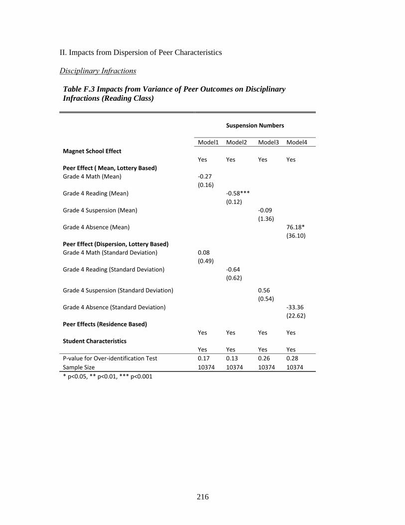
216

II. Impacts from Dispersion of Peer Characteristics


Table F.3 Impacts from Variance of Peer Outcomes on Disciplinary Infractions (Reading Class)

Suspension Numbers



Yes Yes Yes Yes



(0.16)

Grade 4 Reading (Mean) ‐0.58***

(0.12)


(1.36)

Grade 4 Absence (Mean) 76.18*

(36.10)



(0.49)


(0.62)


(0.54)


(22.62)


Yes Yes Yes Yes


Yes Yes Yes Yes


Sample Size 10374 10374 10374 10374

* p<0.05, ** p<0.01, *** p<0.001

217

Absence Rate

Table F.4 Impacts from Variance in Peer Outcomes on Absence Rate (Reading Class) Absence Rate



Yes Yes Yes Yes



(0.00)


(0.00)


(0.03)


(0.87)



(0.00)

Grade 4 Reading (Standard Deviation) 0.00

(0.02)


(0.01)


(0.55)


Yes Yes Yes Yes


Yes Yes Yes Yes


Sample Size 10374 10374 10374 10374

* p<0.05, ** p<0.01, *** p<0.001

218

III. Heterogeneous Peer Effects


Table F.5 Heterogeneous Class Level Peer Effects on Disciplinary Infractions (Reading Class) Suspension Numbers


Black LSES Female



Low Math achiever

High Math Achiever


Proportion Black Students

Mean Effect 0.54** 0.54** 1.11*** 0.76** 0.81*** 0.75** 0.79**

(0.27) (0.25) (0.25) (0.24) (0.24) (0.24) (0.24)

Heterogeneous Effect 0.64** 1.21*** ‐0.59*** 0.19* 0.05 0.21*** 0.2

(0.20) (0.20) (0.15) (0.08) (0.14) (0.08) (0.13)


Mean Effect 0.63* 0.65* 1.43*** 0.93*** 1.04*** 0.90*** 1.02***

(0.27) (0.27) (0.27) (0.26) (0.26) (0.26) (0.26)

Heterogeneous Effect 1.11*** 1.46*** ‐0.77*** 0.27*** ‐0.05 0.32*** 0.05

(0.21) (0.26) (0.18) (0.10) (0.17) (0.10) (0.16)


Mean Effect ‐0.12 ‐0.14 ‐0.37* ‐0.20 ‐0.26 ‐0.22 ‐0.29

(0.18) (0.18) (0.18) (0.18) (0.17) (0.18) (0.17)

Heterogeneous Effect ‐0.47*** ‐0.77*** 0.25** ‐0.21** 0.14 ‐0.13 0.15*

(0.09) (0.11) (0.08) (0.08) (0.07) (0.08) (0.06)


Mean Effect ‐0.42* ‐0.45** ‐0.66*** ‐0.53*** ‐0.58*** ‐0.53*** ‐0.59***

(0.13) (0.13) (0.13) (0.13) (0.12) (0.13) (0.12)

Heterogeneous Effect ‐0.44*** ‐0.61*** 0.17** ‐0.13 0.08 ‐0.11 0.12*

(0.08) (0.09) (0.07) (0.07) (0.06) (0.06) (0.05)


Mean Effect ‐0.20 0.5 1.55** 0.66 1.16** 0.52 1.07*

(0.55) (0.57) (0.49) (0.53) (0.45) (0.53) (0.45)

Heterogeneous Effect 2.48*** 1.24* ‐0.98 0.91* ‐0.36 1.17** 0.29

(0.55) (0.57) (0.50) (0.38) (0.76) (0.41) (0.64)


Mean Effect 11.27 54.71*** 26.61* 44.48** 45.30** 44.51** 44.98**

(13.28) (15.60) (11.80) (15.49) (15.64) (15.60) (15.70)

Heterogeneous Effect 95.09*** ‐34.14 33.84* 2.39 ‐0.19 1.57 1.01

(20.50) (20.42) (16.11) (1.48) (1.93) (1.48) (1.81)

* p<0.05, ** p<0.01, *** p<0.001

219

Absence Rate

Table F.6 Heterogeneous Class Level Peer Effects on Attendance Behavior (Reading Class) Absence Rate


Black LSES Female



Low Math Achiever

High Math Achiever


Proportion Black Students

Mean Effect 0.01 0.01 0.01* 0.01 0.01 0.01 0.01

(0.01) (0.01) (0.01) (0.01) (0.01) (0.01) (0.01)

Heterogeneous Effect ‐0.01 ‐0.00 ‐0.01** 0.00 0.00 ‐0.00 0.00

(0.00) (0.00) (0.00) (0.00) (0.00) (0.00) (0.00)


Mean Effect 0.01 0.01 0.01 0.01 0.01 0.01 0.01

(0.01) (0.01) (0.01) (0.01) (0.01) (0.01) (0.01)

Heterogeneous Effect ‐0.00 0.00 ‐0.01 0.00 0.00 ‐0.00 0.00

(0.01) (0.01) (0.00) (0.00) (0.00) (0.00) (0.00)


Mean Effect ‐0.00 ‐0.00 ‐0.00 ‐0.00 ‐0.00 ‐0.00 ‐0.00

(0.00) (0.00) (0.00) (0.00) (0.00) (0.00) (0.00)

Heterogeneous Effect ‐0.00 ‐0.00 0.00 ‐0.00 0.00* ‐0.00 0.00

(0.00) (0.00) (0.00) (0.00) (0.00) (0.00) (0.00)


Mean Effect ‐0.00 ‐0.00 ‐0.01 ‐0.00 ‐0.00 ‐0.00 ‐0.01

(0.00) (0.00) (0.00) (0.00) (0.00) (0.00) (0.00)

Heterogeneous Effect 0.00 ‐0.00 0.00 ‐0.00 0.00 ‐0.00 0.00

(0.00) (0.00) (0.00) (0.00) (0.00) (0.00) (0.00)


Mean Effect 0.01 0.01 0.02 0.01 0.02 0.02 0.02

(0.01) (0.01) (0.01) (0.01) (0.01) (0.01) (0.01)

Heterogeneous Effect 0.02 0.02 ‐0.01 0.02* 0.02 ‐0.00 ‐0.02

(0.01) (0.02) (0.01) (0.01) (0.02) (0.01) (0.02)


Mean Effect ‐0.63* ‐0.26 ‐0.56* ‐0.45 ‐0.45 ‐0.42 ‐0.45

(0.31) (0.38) (0.29) (0.38) (0.38) (0.38) (0.39)


(0.48) (0.50) (0.39) (0.04) (0.05) (0.04) (0.04)

* p<0.05, ** p<0.01, *** p<0.001

220

REFERENCES

Altonji, J. G., Elder, T., and Taber, C. (2005) An Evaluation of Instrumental Variable Strategies for Estimating the Effects of Catholic Schooling. Journal of Human Resources, 40 (4), 791-821. Ammermueller, A. and Pischke, J. (2006) Peer Effects in European Primary Schools: Evidence from PIRLS. IZA Discussion Paper No. 2077. Anderson, A. R., Christenson, S. L., Sinclair, M. F., and Lehr, C. A. (2004) Check & connect: The importance of relationships for promoting engagement with school. Journal of School Psychology, 42(2), 95-113. Angrist, J. D., and Lang, K. (2004) Does School Integration Generate Peer Effects? Evidence from Boston’s METCO Program. American economic review 94(5), 1613-1634. Argys, L. M., Rees, D., Brewer, D. (1996) Detracking America’s Schools: Equity at Zero Cost? Journal of Policy Analysis and Management. 15 (4), 623-645. Betts, J. R. and Shkolnik, J. (2000) The Effects of Ability Grouping on Student Math Achievement and Resource Allocation in Secondary Schools. Economics of Education Review. 19 (1), 1-15. Betts, J. R. and Zau, A. (2004) Peer groups and academic achievement: Panel evidence from administrative data. Unpublished Manuscript. University of California at San Diego. Boozer, M. A., and Cacciola, S. (2001) Inside the ‘Black Box’ of Project STAR: Estimation of Peer Effects Using Experimental Data. Unpublished Manuscript. Yale University Brock, W., and Durlauf, S. (2000) Interactions-Based Models. NBER Technical Working Paper 258. National Bureau of Economic Research. Cambridge, MA. Burk, M. A., and Sass, T. (2004) Classroom Peer Effects and Academic Achievement. Unpublished Manuscript. Florida State University. Case, A. C., and Katz, L. (1991) The Company You Keep: the Effects of Family and Neighborhood on Disadvantaged Youth. NBER Working Paper. National Bureau of Economic Research. Cambridge, MA. Clotfelter, C. T., Ladd, H., and Vigdor, J. (2006) Teacher-Student Matching and the Assessment of Teacher Effectiveness. Journal of Human Resources. XLI(4), 778-820.

221

Coleman, J. S., Campell, E., Hobson, C., McPartland, J., Mood, A., Weinfeld, F., and York, R. (1966) Equality of Educational Opportunity. Washington, D.C.: U.S. Government Printing Office. Cullen, J. B., Jacob, B., and Levitt, S. (2006) The Effect of School Choice on Participants: Evidence from Randomized Lotteries. Econometrica. 74 (5):1191-1230. Cullen, J. B., Jacobs, B. (2007) Is Gaining Access to Selective Elementary Schools Gaining Ground? Evidence from Randomized Lotteries. NBER Working Paper 13443. National Bureau of Economic Research. Cambridge, MA. Davidson, R., and MacKinnon, J. (1993) Estimation and Inference in Econometrics. New York: Oxford University Press Dills, A. K. (2005) Does Cream-Skimming Curdle the Milk? A Study of Peer Effects. Economics of Education Review. 24, 19-28. Duflo, E., Dupas, P., and Kremer, M. (2008) Peer Effects and the Impact of Tracking: Evidence from a Randomized Evaluation in Kenya, NBER Working Paper 14475. National Bureau of Economic Research. Cambridge, MA. Evans, W. N., Oats, W., and Shwab, R., (1992) Measuring Peer Effects: a Study of Teenage Behavior. Journal of Political Economy. 100 (5), 966-991 Evans, William N. and Robert M. Schwab (1995) Finishing High School and Starting College: Do Catholic Schools Make a Difference? Quarterly Journal of Economics 110 (4): 941-974. Fertig, M. (2003) Educational Production, Endogenous Peer Group Formation and Class Composition – Evidence from the PISA 2000 Study, IZA Discussion Paper 714 Figlio, D. N. (2007) Boys named Sue: Disruptive Children and Their Peers, Education Finance and Policy. 2(4), 376-394. Finn, J. D. and Rock, D. (1997) Academic success among students at risk for school failure. Journal of Applied Psychology, 82(92), 221-234 Gamoran, A. (1986). Instructional and institutional effects of ability grouping. Sociology of Education, 59, 185–198. Gaviria, A. and Raphael, S. (2001) School-Based Peer Effects and Juvenile Behavior. The Review of Economics and Statistics, 83(2), 257-268. Goux, Dominique and Eric Maurin (2005) Close Neighbors Matter: Neighborhood Effects on Early Performance at School, Unpublished Manuscript.

222

Hanushek, E. A., Kain, J., Markman,J., and Rivkin, S. (2003) Does Peer Ability Affect Student Achievement? Applied Economics, 18(5), 527-544. Hanushek, Eric A., John Kain, and Steven Rivkin (2009) New Evidence about Brown v. Board of Education: The Complex Effects of School Racial Composition on Achievement. Journal of Labor Economics, 27(3), 349-383. Henderson, V., Mieszkowski, P., and Sauvageau, Y. (1978) Peer Group Effects and Educational Production Functions. Journal of Public Economics, 10, 97-106 Howell, W. G. and Peterson P. (2002) The Education Gap: Vouchers and Urban Schools. Washington, DC: Brookings Institution Press. Hoxby, C. M. (2000) Peer Effects in the Classroom: Learning from Gender and Race Variation. NBER Working Paper 7867. National Bureau of Economic Research. Cambridge, MA. Hoxby, Caroline M. (2000) Does Competition among Public Schools Benefit Students And Taxpayers, American Economic Review 90(5): 1209-1238 Imbernman, S., Kuglar, A., and Sacerdote, B. (2009) Katrina’s Children: Evidence on the Structure of Peer Effects from Hurricane Evacuees. NBER Working Paper 15291. National Bureau of Economic Research. Cambridge, MA. Ingersoll, R. (1999) The Problems of Underqualified Teachers in American Secondary Schools. Educational Researcher, 28(2): 26-37 Ingersoll, R. (2004) Why Do High-Poverty Schools Have Difficulty Staffing Their Classrooms with Qualified Teachers? Working Paper, University of Pennsylvania Kang, C. (2007) Classroom Peer Effects and Academic Achievement: Quasi- Randomization Evidence from South Korea. Journal of Urban Economics, 61, 458-495. Katz, L. F., Kling, J. R., and Liebman, J. (2001) Moving to Opportunity in Boston: Early Results of a Randomized Mobility. Quarterly Journal of Economics, 116 (2), 607-654. Kremer, M, and Levy D. (2003) Peer effects and alcohol use among college students. NBER Working Paper 9876, National Bureau of Economic Research. Cambridge, MA. Krueger, A. (1999) Experimental Estimates of Education Production Functions. Quarterly Journal of Economics 114(2), 497–532. Lamdin, D. J. (1996) Evidence of student attendance as an independent variable in education production functions. Journal of Educational Research, 89, 155-162.

223

Lavy, V., and Shlosser, A. (2007) Mechanisms and Impacts of Gender Peer Effects at School. NBER Working Paper 13292. National Bureau of Economic Research. Cambridge, MA. Lazear, E. P. (2001) Educational production Function. Quarterly Journal of Economics 116, 777–803. Lefgren, L. (2004) Educational peer effects and the Chicago public schools. Journal of Urban Economics. 56, 169–191. Manski, C. F. (1993) Identification of Endogenous Social Effects: the Reflection Problem. The Review of Economic Studies. 60(3), 531-542 Manski, C. F. (1999) Identification Problems in the Social Sciences. Cambridge, MA.: Harvard University Press Manski, C. F. (2000) Economic Analysis of Social Interactions. Journal of Economic Perspectives. 14(3), 115-136. McEwan P. J. (2003) Peer Effects on Student Achievement: Evidence from Chile. Economics of Education Review. 22, 131-141 Mickelson, R. A. (2001). Subverting Swann: Tracking and second generation segregation in Charlotte-Mecklenburg Schools. American Education Research Journal, 38, 215–252. Moffit, R. A. (2001) Policy Interventions, Low-Level Equilibria, and Social Interactions. in: Durlauf, S. and Young, P. (Eds) Social Dynamics. MIT Press, Cambridge, MA, 2001, pp. 45–82. Neal, D. (1997) The Effects of Catholic Secondary Schooling on Educational Attainment, Journal of Labor Economics, 15, 98-123. Oaks, J. (1992) Can Tracking Research Inform Practice? Technical, Normative, and Political Considerations. Educational Researcher, 21(4), 12-21. Peske H.G., and Haycock, K. (2006) Teaching Inequality: How Poor and Minority Students Are Shortchanged on Teacher Quality. Education Trust Report. Education Trust. Washington, D.C. Peterson, P. (1998) School choice: A report card. In P. Peterson & B. Hassel (Eds.), Learning from school choice (pp. 3-32). Washington, DC: Brookings Institution Rivkin, S. G. (2001) Tiebout sorting, aggregation and the estimation of peer group effects. Economics of Education Review. 20, 201-209

224

Rouse, C. E. (1998) Private School Vouchers and Student Achievement: An Evaluation ofthe Milwaukee Parental Choice Program, Quarterly Journal of Economics 113 (2), 553-602. Rowley, K. J. (2005) Setting Boundaries: Monitoring the effects of closer-to-home school rezoning on student participation & engagement in school. Ph.D. diss. Vanderbilt University Rumberger, R. W. (1995) Dropping out of middle school: A multilevel analysis of students and schools. American Educational Research Journal, 23(3), 583-625. Sacerdote, B. (2001) Peer effects with random assignment: Results for Dartmouth roommates. Quarterly Journal of Economics. 116, 681–704. Smrekar, C., & Goldring, E., (1999) School Choice in Urban America: Magnet schools and the Pursuit of Equity. New York: Teachers College Press. Stinebrickner T., and Stinebrickner, R. (2001) Peer Effects Among Students from Disadvantaged Backgrounds. CIBC Human Capital and Productivity Project Working Papers 20013. University of Western Ontario. Stiefel, L., Schwartz, A., and Zabel, J. (2004) The Impact of Peer Effects on Student Outcomes in New York City Public Schools, Unpublished Manuscript. Summers, A., and Wolfe B. (1977) Do Schools Make a Difference? American Economic Review. 67, 639-650. Sund, K. (2009) Estimating peer effects in Swedish high school using school, teacher, and student fixed effects. Economics of Education Review, 28(3), 329-336. Vigdor, J., and Nechyba, T. (2004) Peer Effects in North Carolina Public Schools. Unpublished Manuscript. Duke Univeristy. Vigdor, J., and Nechyba, T. (2008) Causal Inference when Assignment May Have Been Random: Peer Effects in North Carolina Elementary schools. Unpublished Manuscript. Duke Univeristy.

Wentzel, K. R. (1993) Does Being Good Make the Grade? Social Behavior and Academic Competence in Middle School. Journal of Educational Psychology, 85(2), 357-364.

Wentzel, K. R., Weinberger, D. A., Ford, M. E., & Feldman, S. S.(1990) Academic achievement in preadolescence: The role ofmotivational, affective, and self-regulatory processes. Journal of Applied Developmental Psychology, 11, 179-193.

Winkler, D. R.(1975) Educational Achievement and School Peer Group Composition. The Journal of Human Resources, 10(2), 189-204.

225

Wooldridge, J. M. (2001) Econometric Analysis of Cross Section and Panel Data. Cambridge, Massachusetts: The MIT Press Zimmerman, D. J. (2003) Peer effects in academic outcomes: Evidence from a natural experiment, Review of Economics and Statistics. 85, 9–23.

EVIDENCE FROM RANDOMIZED LOTTERIES...

Documents

Transcript of EVIDENCE FROM RANDOMIZED LOTTERIES...