Evidence for Monetary Non-Neutrality -...
92
E VIDENCE FOR MONETARY NON-NEUTRALITY Emi Nakamura and Jon Steinsson Columbia University March 2018 Nakamura-Steinsson (Columbia) Monetary Non-Neutrality 1 / 64
Transcript of Evidence for Monetary Non-Neutrality -...

EVIDENCE FOR MONETARY NON-NEUTRALITY
Emi Nakamura and Jon Steinsson
Columbia University
March 2018
Nakamura-Steinsson (Columbia) Monetary Non-Neutrality 1 / 64

EFFECTS OF MONETARY POLICY?
Central question in macroeconomics:
1. Monetary policy is a central macroeconomic policy tool
2. Answer helps distinguish between competing views of
how the world works more generally (Why?)
Consensus within mainstream U.S. media that effects are large
No consensus in many other countries
Much controversy in academia
(Often quite heated and antagonistic)
Scientific question!!
Conclusive empirical evidence should be able to settle this issue
(for those willing to base opinion on evidence as opposed to ideology)
Nakamura-Steinsson (Columbia) Monetary Non-Neutrality 2 / 64

WHY DON’T WE ALREADY KNOW?
Given central importance, how can we not already know?
Changes in monetary policy occur for a reason!!
Purpose of central banks to conduct systematic policy
that reacts to developments in economy
Fed employs hundreds of PhD economists to pore over data
Leaves little room for exogenous variation in policy
needed to identify effects of policy
Nakamura-Steinsson (Columbia) Monetary Non-Neutrality 3 / 64

ENDOGENEITY OF MONETARY POLICY
Fed lowered interest rates aggressively in fall of 2008
Done in response to worsening financial crisis
Consider simple OLS regression:
∆yt = α + β∆it + εt
This regression will not identify effects of policy
Financial crisis – event that induced Fed to act – is a confounding factor
(in error term and correlated with ∆it )
Nakamura-Steinsson (Columbia) Monetary Non-Neutrality 4 / 64

WHAT IS THE BEST EVIDENCE WE HAVE?
When we ask prominent macroeconomists, most common answers are:1
Friedman and Schwartz 63
Volcker disinflation
Mussa 86
1Of course, a significant fraction say something along the lines of “I know it in my bones thatmonetary policy has no effect on output.”
Nakamura-Steinsson (Columbia) Monetary Non-Neutrality 5 / 64
TYPES OF EVIDENCE
Evidence from Large Shocks
Discontinuity-Based Evidence / High-Frequency Evidence
Evidence from the Narrative Record
Controlling for Confounding Factors
Structural Vector Autoregressions
Romer and Romer (2004)
Nakamura-Steinsson (Columbia) Monetary Non-Neutrality 6 / 64

Evidence from Large Shocks
FRIEDMAN-SCHWARTZ 63
Three policy actions that were:
1. “Of major magnitude”
2. “Cannot be regarded as necessary or inevitable economic
consequences of contemporary changes in money income and prices.”
These were:
1. January - June 1920
2. October 1931
3. July 1936 - January 1937
We focus on second two – which occurred during the Great Depression
Nakamura-Steinsson (Columbia) Monetary Non-Neutrality 7 / 64

INDUSTRIAL PRODUCTION IN U.S. GREAT DEPRESSION
4080
120
160
1925 1930 1935 1940Year
Nakamura-Steinsson (Columbia) Monetary Non-Neutrality 8 / 64
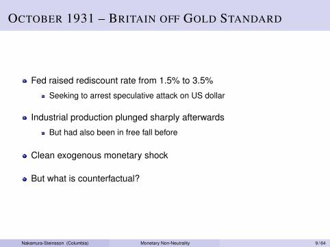
OCTOBER 1931 – BRITAIN OFF GOLD STANDARD
Fed raised rediscount rate from 1.5% to 3.5%
Seeking to arrest speculative attack on US dollar
Industrial production plunged sharply afterwards
But had also been in free fall before
Clean exogenous monetary shock
But what is counterfactual?
Nakamura-Steinsson (Columbia) Monetary Non-Neutrality 9 / 64

JULY 36 - JANUARY 37 – MISTAKE OF 1937
Fed announced doubling of reserve requirements and
Treasury sterilized gold inflows
Strong growth before, sharp plunge afterwards
Confounding factors?
Fiscal policy was tight in 1937
(end or veteran’s bonuses and first collection of social security tax)
Great deal of labor unrest in 1937
Nakamura-Steinsson (Columbia) Monetary Non-Neutrality 10 / 64

FRIEDMAN-SCHWARTZ 63 AND GREAT DEPRESSION
More general argument: Fed caused the Depression by failing to act
Fed stood by and let money supply collapsed (largely due to banking
failures) and economy collapsed as a consequence
If Benjamin Strong had not died, Great Depression would have been
a mild recession
Eichengreen 92 argues policy was constrained by gold standard
Roosevelt took US off gold standard in April 1933(black line in figure above)
Timing suggests that something Roosevelt did mattered
But Roosevelt did several things
Nakamura-Steinsson (Columbia) Monetary Non-Neutrality 11 / 64

GOLD STANDARD AND GREAT DEPRESSION
Countries that left the gold standard earlier did better
(Choudhri-Kochin 80, Eichengreen-Sachs 85)
Nakamura-Steinsson (Columbia) Monetary Non-Neutrality 12 / 64

936 Eichengreen and Sachs
Industrial Production
1935 (1929= 100)
130 .
. FINLAND DENf4ARK
120- SWEDEN
UNITED KINGDOM
110 - * NORWAY
100-\ *GERMANY
* ITALY
90- *NETHERLANDS
IP 1935= 153.9 - 0.69 ER 1935
80-\
*BELGIUM *FRANCE 70 I I1
40 6'0 8'0 100 120 Exchange Rate
1935 (I1929 = 100)
FIGURE 1 CHANGES IN EXCHANGE RATES AND INDUSTRIAL PRODUCTION, 1929-1935
plotted along the horizontal axis, is expressed as the gold price of domestic currency in 1935 as a percentage of the 1929 parity; a value of 100 for France indicates no depreciation, while a value of 59 for the United Kingdom indicates a 41 percent depreciation. The change in industrial production, plotted along the vertical axis, is the ratio of production in 1935 to 1929 multiplied by 100.
There is a clear negative relationship between the height of the exchange rate and the extent of recovery from the Depression. The countries of the Gold Bloc, represented here by France, the Nether- lands, and Belgium, had by 1935 failed to recover to 1929 levels of industrial production. Countries which devalued at an early date (the United Kingdom, Denmark, and the Scandinavian countries) grew much more rapidly; and there appears to be a positive relationship between the magnitude of depreciation and the rate of growth. Germany
different implications for the characteristics of both the downturn and the recovery. We did no experimentation with different samples of countries but intend to increase the size of the sample in future work.
This content downloaded from 128.59.160.114 on Fri, 13 Feb 2015 14:28:10 PMAll use subject to JSTOR Terms and Conditions
Source: Eichengreen and Sachs (1985)
Nakamura-Steinsson (Columbia) Monetary Non-Neutrality 13 / 64

GOLD STANDARD AND GREAT DEPRESSION
But countries don’t leave the gold standard randomly
Countries that were forced off gold earlier likely had
“weaker” fundamentals
Suggests causal relationship may be even stronger
Nakamura-Steinsson (Columbia) Monetary Non-Neutrality 14 / 64
GOLD STANDARD AND GREAT DEPRESSION
But countries don’t leave the gold standard randomly
Countries that were forced off gold earlier likely had
“weaker” fundamentals
Suggests causal relationship may be even stronger
Nakamura-Steinsson (Columbia) Monetary Non-Neutrality 14 / 64

VOLCKER DISINFLATION
24
68
10
05
1015
20
1970 1975 1980 1985 1990 1995Year
Blue: Fed funds rate (left). Red: 12-month inflation (left). Green: Unemployment (right).
Nakamura-Steinsson (Columbia) Monetary Non-Neutrality 15 / 64

VOLCKER DISINFLATION
Volatile and rising inflation in the 1970s
“Stop-go” policy (e.g., Goodfriend 07)
August 79, Paul Volcker takes over as Chair of Fed:
Oct 79 - Mar 80: Very tight policy
Apr 80 - Nov 80: Loose policy
Nov 80 - Late 82: Very tight policy
Economy swings with monetary policy:
Spring-Summer 80: Output fell dramatically
Late 80: Output rebounds, inflation still high (stop-go)
1981-1982: Output falls, large recession, inflation down
Nakamura-Steinsson (Columbia) Monetary Non-Neutrality 16 / 64

Discontinuity-Based Evidence

MONETARY POLICY AND RELATIVE PRICES
Strong evidence for effects of monetary policy on relative prices
Important reason: Can be assessed using discontinuity-based
identification
Nakamura-Steinsson (Columbia) Monetary Non-Neutrality 17 / 64

MUSSA 86 – BREAKDOWN OF BRETTON WOODS
-15
-10
-50
510
15Percent
1960 1965 1970 1975 1980 1985Year
Change in U.S. - German real exchange rate.
Nakamura-Steinsson (Columbia) Monetary Non-Neutrality 18 / 64

MONETARY POLICY AND REAL EXCHANGE RATE
Bretton Woods system of fixed exchange rates breaks down in Feb 73
This is a pure high-frequency change in monetary policy
Sharp break in volatility of real exchange rate
Identifying assumption:
Nothing else changed discontinuously in Feb 73
Imbalances had been building up gradually
More inflationary policy in US than in Germany, Japan, etc.
US running substantial current account deficit
Intense negotiations for months about future of system
Hard to see anything else that discontinuously changes in Feb 73
Nakamura-Steinsson (Columbia) Monetary Non-Neutrality 19 / 64

MONETARY POLICY AND REAL INTEREST RATES
High-frequency evidence on real interest rates:
Look at narrow time windows around FOMC announcements
Measure real interest rate using yields on TIPS
Identifying assumption:
Little else happens during narrow window (30-minutes)
Changes must be due to what Fed did and announced
Nominal and real rates respond roughly one-for-one several years
into term structure (see, e.g., Nakamura-Steinsson 17, Hansen-Stein 15)
We will return to this next week
Nakamura-Steinsson (Columbia) Monetary Non-Neutrality 20 / 64

EVIDENCE ON RELATIVE PRICES
Advantages:
Effect on relative prices can be estimated using
discontinuity-based approaches
Disadvantages:
No direct link to output
Effects depend on how we interpret price changes
(information, risk premia)
Effect on output depends on various other parameters
in the “real” model (e.g., IES)
Nakamura-Steinsson (Columbia) Monetary Non-Neutrality 21 / 64

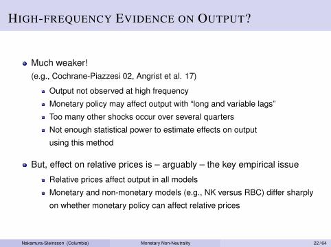
HIGH-FREQUENCY EVIDENCE ON OUTPUT?
Much weaker!(e.g., Cochrane-Piazzesi 02, Angrist et al. 17)
Output not observed at high frequency
Monetary policy may affect output with “long and variable lags”
Too many other shocks occur over several quarters
Not enough statistical power to estimate effects on output
using this method
But, effect on relative prices is – arguably – the key empirical issue
Relative prices affect output in all models
Monetary and non-monetary models (e.g., NK versus RBC) differ sharply
on whether monetary policy can affect relative prices
Nakamura-Steinsson (Columbia) Monetary Non-Neutrality 22 / 64

Evidence from the Narrative Record

NARRATIVE EVIDENCE – ROMER-ROMER 89
Romer-Romer 89:
Fed records can be used to identify natural experiments
Specifically: “Episodes in which the Federal Reserve attempted to exert
a contractionary influence on the economy in order to reduce inflation.”
Six episodes (Romer-Romer 94 added a seventh)
After each one, unemployment rises sharply
Strong evidence for substantial real effects of monetary policy
(Paper also contains an interesting critical assessment of Friedman-Szhwartz 63)
Nakamura-Steinsson (Columbia) Monetary Non-Neutrality 23 / 64
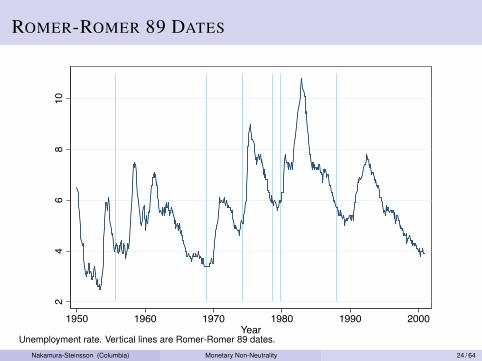
ROMER-ROMER 89 DATES
24
68
10
1950 1960 1970 1980 1990 2000Year
Unemployment rate. Vertical lines are Romer-Romer 89 dates.
Nakamura-Steinsson (Columbia) Monetary Non-Neutrality 24 / 64

ROMER-ROMER 89 – CRITIQUES
Inherent opacity of the process of selecting the shock dates
High cost of replication
Similar critique applies to many complex econometric methods
Few data points
May happen to be correlated with other shocks
Hoover-Perez 94 point out high correlation with oil shocks
Shocks predictable suggesting endogeneity
Difficult to establish convincingly due to overfitting concerns
Cumulative number of predictability regressions run hard to know
Nakamura-Steinsson (Columbia) Monetary Non-Neutrality 25 / 64

Table A.1: Romer-Romer Dates and Oil-Shock Dates
Romer and Romer Dates Oil Shock Dates
October 1947 December 1947
June 1953
September 1955 June 1956
February 1957
December 1968 March 1969
December 1970
April 1974 January 1974
August 1978 March 1978
October 1979 September 1979
February 1981
January 1987
December 1988 December 1988
August 1990
Notes: Romer-Romer dates are dates are identified by Romer and Romer (1989) and Romerand Romer (1994). Oil-shock dates up to 1981 are taken from Hoover and Perez (1994),who refine the narrative identification of these shocks by Hamilton (1983). The last three oilshock dates are from Romer and Romer (1994).
37
Source: Nakamura and Steinsson (2018)
Nakamura-Steinsson (Columbia) Monetary Non-Neutrality 26 / 64

Controlling for Confounding Factors
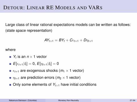
DETOUR: LINEAR RE MODELS AND VARS
Large class of linear rational expectations models can be written as follows:
(state space representation)
AYt+1 = BYt + Cεt+1 + Dηt+1
where
Yt is an n × 1 vector
E [εt+1|It ] = 0, E [ηt+1|It ] = 0
εt+1 are exogenous shocks (m1 × 1 vector)
ηt+1 are prediction errors (m2 × 1 vector)
Only some elements of Yt+1 have initial conditions
Nakamura-Steinsson (Columbia) Monetary Non-Neutrality 27 / 64
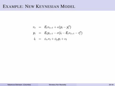
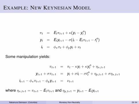
EXAMPLE: NEW KEYNESIAN MODEL
πt = Etπt+1 + κ(yt − ynt )
yt = Etyt+1 − σ(it − Etπt+1 − rnt )
it = φππt + φy yt + νt
Some manipulation yields:
πt+1 = πt − κyt + κynt + ηπ,t+1
yt+1 + σπt+1 = yt + σit − σrnt + ηy,t+1 + σηπ,t+1
it+1 − φππt+1 − φy yt+1 = νt+1
where ηπ,t+1 = πt+1 − Etπt+1 and ηy,t+1 = yt+1 − Etyt+1
Nakamura-Steinsson (Columbia) Monetary Non-Neutrality 28 / 64
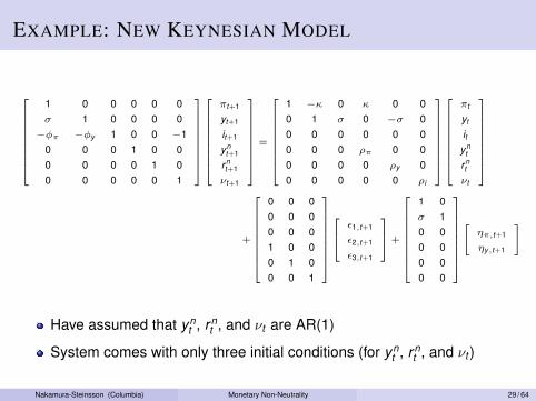
EXAMPLE: NEW KEYNESIAN MODEL
1 0 0 0 0 0σ 1 0 0 0 0
−φπ −φy 1 0 0 −10 0 0 1 0 00 0 0 0 1 00 0 0 0 0 1
πt+1
yt+1
it+1
ynt+1
rnt+1
νt+1
=
1 −κ 0 κ 0 00 1 σ 0 −σ 00 0 0 0 0 00 0 0 ρπ 0 00 0 0 0 ρy 00 0 0 0 0 ρi
πt
yt
ityn
t
rnt
νt
+
0 0 00 0 00 0 01 0 00 1 00 0 1
ε1,t+1
ε2,t+1
ε3,t+1
+
1 0σ 10 00 00 00 0
[ηπ,t+1
ηy,t+1
]
Have assumed that ynt , rn
t , and νt are AR(1)
System comes with only three initial conditions (for ynt , rn
t , and νt )
Nakamura-Steinsson (Columbia) Monetary Non-Neutrality 29 / 64

SOLVING LINEAR RATIONAL EXPECTATIONS MODELS
State space representation:
AYt+1 = BYt + Cεt+1 + Dηt+1
Solution:
Yt = GYt−1 + Rεt
How to solve?
Blanchard-Kahn 80. See, e.g., Sims 00 or lecture notes by Den Haan
Notice: Solution of a linear RE model is a VAR
Nakamura-Steinsson (Columbia) Monetary Non-Neutrality 30 / 64

IMPULSE RESPONSE FUNCTIONS
Suppose we are interested in effect of ε3,0 on yt for t ≥ 0
(Recall that ε3,0 is the innovation to the monetary shock)
Iterate forward the VAR starting at time 0:
Yt = GtY−1 + Gt−1Rε0
Suppose for simplicity that we start off in a steady state Y−1 = 0:
Yt = Gt−1Rε0
If we can estimate G and R, then we can calculate
dynamic causal effect of all structural shocks
Nakamura-Steinsson (Columbia) Monetary Non-Neutrality 31 / 64

VAR ESTIMATION: EMPIRICAL CHALLENGES
Yt = GYt−1 + Rεt
1. Some variables in true VAR may be unobservable
In NK model example, (ynt , r n
t , and νt ) are unobservable
How about solving out for these variables?
This typically transforms a VAR(p) into a VARMA(∞,∞)
Implicit assumption in VAR estimation that true VARMA(∞,∞) in
observable variables can be approximated by a VAR(p)
(Problem Set 3 will have you think more about this)
Nakamura-Steinsson (Columbia) Monetary Non-Neutrality 32 / 64

VAR ESTIMATION: EMPIRICAL CHALLENGES
Yt = GYt−1 + Rεt
2. How do we get from reduced form errors to structural errors?
Suppose you estimate a VAR (i.e., estimate n OLS regressions)
You will get:
Yt = GYt−1 + ut
where ut are reduced form errors with variance-covariance matrix Σ
Unfortunately, Σ not enough to identify R
Structural VARs make additional assumptions to be able to identify R
Two ways of thinking about it: Identification of R or identification of
structural shocks εt
Nakamura-Steinsson (Columbia) Monetary Non-Neutrality 33 / 64

DYNAMIC CAUSAL INFERENCE
Objective:
Causal effect of change in monetary policy at time t
on output / prices / etc. at time t + j
Two steps:
1. Identify shocks (exogenous variation in (say) monetary policy)
2. Estimate effects of shocks on output / prices / etc.
Important to consider these two steps separately
Nakamura-Steinsson (Columbia) Monetary Non-Neutrality 34 / 64

SVAR IDENTIFICATION OF MONETARY SHOCKS
Common approach:
Regress fed funds rate on output, inflation, etc. + a few lags of
fed funds rate, output, inflation, etc.
it = α + φy yt + φππt + [four lags of it , yt , πt ] + εt
View residual as exogenous variation in monetary policy
Equivalent to performing a Cholesky decomposition on reduced form
errors from VAR, ordering fed funds rate last (See Stock-Watson 01)
Nakamura-Steinsson (Columbia) Monetary Non-Neutrality 35 / 64

SVARS: IDENTIFYING THE SHOCKS
it = α + φy yt + φππt + [four lags of it , yt , πt ] + εt
What can go wrong?
1. Reverse causation:
Assumption begin made: Correlation between it and (πt , yt ) is due to
(πt , yt ) influencing it but not the other way around
If it influences (πt , yt ) (contemporaneously), we have a
“simultaneous equation problem” (εt correlated with (πt , yt ))
Assumption being made: it is “fast-moving” variable, while πt and yt are
slow moving. So it doesn’t affect πt and yt contemporaneously
Often, the discussion of identification stops here and seems surprisingly
inocuous. Where did the rabbit go into the hat?
Nakamura-Steinsson (Columbia) Monetary Non-Neutrality 36 / 64

SVARS: IDENTIFYING THE SHOCKS
it = α + φy yt + φππt + [four lags of it , yt , πt ,etc.] + εt
What can go wrong?
2. Omitted variables bias:
There may be other variables that affect it and also yt+j
Fed bases policy on huge amount of data
Banking sector, stock market, foreign developments, commodity prices,terrorist attacks, temporary investment tax credit, Y2K, etc., etc.
Too many variables to include in regression!
Any information used by Fed and not sufficiently controlled for by
included controls will result in endogenous variation in policy being
viewed as exogenous shock to policy
Nakamura-Steinsson (Columbia) Monetary Non-Neutrality 37 / 64

WAS 9/11 A MONETARY SHOCK?
3 Jan*
31 Jan
20 Mar
18 Apr*
15 May
27 Jun21 Aug
17 Sep*
2 Oct
6 Nov
11 Dec23
45
67
Perc
ent
Dec Jan Feb Mar Apr May Jun Jul Aug Sep Oct Nov Dec Jan Feb Mar
21 Aug
17 Sep*
2 Oct
22.
53
3.5
4Pe
rcen
t
Aug Sep Oct Nov
Dark line: Fed funds target. Light line/dots: 1-month eurodollar rate. * indicates unscheduled meeting.Sample period: Dec 2000 - Feb 2002.
Nakamura-Steinsson (Columbia) Monetary Non-Neutrality 38 / 64
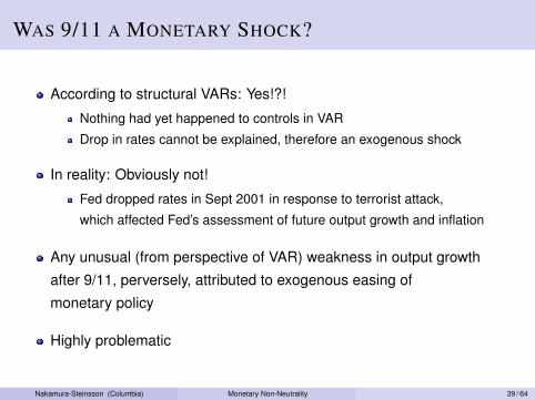
WAS 9/11 A MONETARY SHOCK?
According to structural VARs: Yes!?!
Nothing had yet happened to controls in VAR
Drop in rates cannot be explained, therefore an exogenous shock
In reality: Obviously not!
Fed dropped rates in Sept 2001 in response to terrorist attack,
which affected Fed’s assessment of future output growth and inflation
Any unusual (from perspective of VAR) weakness in output growth
after 9/11, perversely, attributed to exogenous easing of
monetary policy
Highly problematic
Nakamura-Steinsson (Columbia) Monetary Non-Neutrality 39 / 64
IDENTIFYING ASSUMPTIONS IN SVARS
“The” identifying assumption in a monetary VAR often described as:
Fed funds rate does not affect output, inflation, etc. contemporaneously
Seems like magic:
You make one relatively innocuous assumption
Violá: You can estimate dynamic causal effects of monetary policy
Nakamura-Steinsson (Columbia) Monetary Non-Neutrality 40 / 64

IDENTIFYING ASSUMPTIONS IN SVARS
Timing assumption not only identifying assumption being made
Timing assumption rules out reverse causality
Contemporaneous correlation assumed to go from output to interest rates
Not other way around
Bigger concern: Omitted variables bias
Monetary policy and output may be reacting to some other shock
If not sufficiently proxied by included controls, this shock will cause
omitted variables bias (e.g., 9/11)
Nakamura-Steinsson (Columbia) Monetary Non-Neutrality 41 / 64

ROMER-ROMER 04
Hopeless to control individually for everything in Feds information set
Alternative approach:
Control for Fed’s own forecasts (Greenbook forecasts)
Key idea:
Endogeneity of monetary policy comes from one thing only:
What Fed thinks will happen to the economy
Controlling for this is sufficient
Nakamura-Steinsson (Columbia) Monetary Non-Neutrality 42 / 64

CONSTRUCTING THE SHOCKS SERIES
Romer-Romer’s shock series addresses two problems:
1. Fed has imperfect control over fed funds rate
More of a problem before Greenspan era
Movements in FFR relative to FOMC target are endogenous
(FFR rises relative to target in response to good news about future output)
Romer-Romer construct FFR target series
2. Movements in FOMC’s FFR target are endogenous
“Anticipatory effects” important
(e.g., Fed lowers rates in anticipation of economic weakness)
Use of Fed’s Greenbook forecasts control for such endogeneity
(Greenbook typically prepared six days before meeting)
Nakamura-Steinsson (Columbia) Monetary Non-Neutrality 43 / 64

CONTROLLING FOR GREENBOOK FORECAST
Romer-Romer’s specification:
∆ffm = α + βffbm +2∑
i=−1
γi ∆ymi +2∑
i=−1
λi (∆ymi −∆ym−1,i )
+2∑
i=−1
φi πmi +2∑
i=−1
θi (πmi − πm−1,i ) + ρum0 + εm
∆ffm change in intended FFR at meeting
ffbm level before meeting
y , π, u forecasts of output, inflation, and unemployment
Both forecasts and change in forecasts since last meeting included
Nakamura-Steinsson (Columbia) Monetary Non-Neutrality 44 / 64

DOES THIS MAKE SENSE?
Residual εm considered exogenous monetary policy shock
Does this make sense?
Romer and Romer:It is important to note that the goal of this regression is not to es-
timate the Federal Reserve’s reaction function as well as possible.
What we are trying to do is to purge the intended funds rate series
of movements taken in response to useful information about future
economic developments. Once we have accomplished this, it is de-
sirable to leave in as much of the remaining variation as possible.
Nakamura-Steinsson (Columbia) Monetary Non-Neutrality 45 / 64

COCHRANE (2004)
Proposition 1: To measure the effects of monetary policy on out-put it is enough that the shock is orthogonal to output forecasts.
The shock does not have to be orthogonal to price, exchange rate
or other forecasts. It may be predictable from time t information; it
does not have to be a shock to agent’s or the Fed’s entire informa-
tion set.
(no proof provided)
All the shock has to do is remove the reverse causality from output
forecasts.
Nakamura-Steinsson (Columbia) Monetary Non-Neutrality 46 / 64

ROMER-ROMER 04 / COCHRANE 04:
WHAT IS A MONETARY SHOCK?
Fed does not roll dice
Every movement in intended fed funds rate is a response to something
Some are responses to something that directly affectsoutcome variable of interest
These are endogenous
Reactions to anything else (exchange rate, political pressure, etc)
conditional on output forecast count as a shock
Nakamura-Steinsson (Columbia) Monetary Non-Neutrality 47 / 64

COCHRANE (2004)
Preferred specification for effects on output:
∆ffm = α +2∑
i=−1
γi ∆ymi + βffm−1 + δ∆ffm−1 + εym
Preferred specification for effects on inflation:
∆ffm = α +2∑
i=−1
γi ∆πmi + βffm−1 + δ∆ffm−1 + επm
Lagged FFR only included to make shocks serially uncorrelated,
which simplifies interpretation
No need to include other controls
In fact, better not to, since this keeps more shocks
Nakamura-Steinsson (Columbia) Monetary Non-Neutrality 48 / 64
ROMER-ROMER IDENTIFICATION REVISITED
Objective:
Causal effect of change in interest rates at time t on output at time t + j
Need exogenous variation in interest rates at time t
Romer-Romer/Cochrane argument:
Change in intended FFR conditional on Fed’s output forecasts
is exogenous
Potential worries:
Reverse causality
Omitted variables bias
Nakamura-Steinsson (Columbia) Monetary Non-Neutrality 49 / 64

REVERSE CAUSALITY
Fed lowers rates because it thinks output is going to be low
For this, Fed’s output forecast is a sufficient statistic,
the only variable you need to control for
Only worry is whether Greenbook forecast is the same as
FOMC forecast
If not, reverse causality may remain
Nakamura-Steinsson (Columbia) Monetary Non-Neutrality 50 / 64

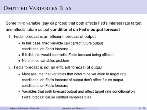
OMITTED VARIABLES BIAS
Some third variable (say oil prices) that both affects Fed’s interest rate target
and affects future output conditional on Fed’s output forecast
1. Fed’s forecast is an efficient forecast of output
In this case, third variable can’t affect future output
conditional on Fed’s forecast
If it did, this would contradict Fed’s forecast being efficient
No omitted variables problem
2. Fed’s forecast is not an efficient forecast of output
Must assume that variables that determine variation in target rate
conditional on Fed’s forecast of output don’t affect future output
conditional on Fed’s forecast
Variables that both forecast output and affect target rate conditional on
Fed’s forecast cause omitted variables bias
Nakamura-Steinsson (Columbia) Monetary Non-Neutrality 51 / 64

WHAT ARE MONETARY SHOCKS?
“Good” variation:
Shifts in the Fed’s preferences or views about how the economy works
Fed cares about other things than just output (dual mandate)
Variables that affect other things that the Fed cares about (but not output)
conditional on output forecasts
“Bad” variation:
Variables that both forecast output and affect target rate
conditional on Fed’s forecast
Nakamura-Steinsson (Columbia) Monetary Non-Neutrality 52 / 64

ROMER-ROMER SHOCKS
Policy makers’ beliefs about the workings ofthe economy are another source of shocks. Forexample, in the early 1970’s the prevailingframework at the Federal Reserve held that in-flation was extremely unresponsive to economicslack (Romer and Romer, 2002). One wouldexpect this belief to lead the Federal Reserve toset lower interest rates than it otherwise wouldhave. And indeed, our shock series is generallynegative in 1971 and 1972.
A third source of shocks are the Federal Re-serve’s tastes and goals. A Federal Reserve thathas a particular distaste for inflation, for exam-ple, is likely to set higher interest rates than ittypically would. Our series shows obvious up-
ward spikes in 1969, 1973–1974, and 1979–1982. These are three periods that we identifiedin previous work as times when the FederalReserve decided that the current level of infla-tion was too high and that it was willing toendure output losses to reduce it (Romer andRomer, 1989).10
10 These policy shifts involved more than mere changesin tastes, and to a large extent reflected changes in theFederal Reserve’s understanding of the economy. Thusthere is not a sharp distinction between shocks coming fromthe Federal Reserve’s beliefs and ones stemming from itstastes.
FIGURE 1. MEASURES OF MONETARY POLICY
1065VOL. 94 NO. 4 ROMER AND ROMER: A NEW MEASURE OF MONETARY SHOCKS
Source: Romer and Romer (2004).Nakamura-Steinsson (Columbia) Monetary Non-Neutrality 53 / 64

Policy makers’ beliefs about the workings ofthe economy are another source of shocks. Forexample, in the early 1970’s the prevailingframework at the Federal Reserve held that in-flation was extremely unresponsive to economicslack (Romer and Romer, 2002). One wouldexpect this belief to lead the Federal Reserve toset lower interest rates than it otherwise wouldhave. And indeed, our shock series is generallynegative in 1971 and 1972.
A third source of shocks are the Federal Re-serve’s tastes and goals. A Federal Reserve thathas a particular distaste for inflation, for exam-ple, is likely to set higher interest rates than ittypically would. Our series shows obvious up-
ward spikes in 1969, 1973–1974, and 1979–1982. These are three periods that we identifiedin previous work as times when the FederalReserve decided that the current level of infla-tion was too high and that it was willing toendure output losses to reduce it (Romer andRomer, 1989).10
10 These policy shifts involved more than mere changesin tastes, and to a large extent reflected changes in theFederal Reserve’s understanding of the economy. Thusthere is not a sharp distinction between shocks coming fromthe Federal Reserve’s beliefs and ones stemming from itstastes.
FIGURE 1. MEASURES OF MONETARY POLICY
1065VOL. 94 NO. 4 ROMER AND ROMER: A NEW MEASURE OF MONETARY SHOCKS
Source: Romer and Romer (2004).Nakamura-Steinsson (Columbia) Monetary Non-Neutrality 54 / 64

WHAT ARE THE SHOCKS?
1. Variation in Fed operating procedure important
E.g., emphasis on monetary quantities in 1979-1982
2. Variation in policy makers’ beliefs about workings of economy
In early 1970’s Fed believed inflation highly unresponsive to slack
(Romer-Romer 02)
3. Variation in policy maker preferences/goals
E.g., time-varying distaste for inflation
4. Political influences
E.g., Arthur Burns set loose policy in 1977 to get re-appointed
5. Pursuit of other objectives
At some times, Fed concerned about exchange rate
Nakamura-Steinsson (Columbia) Monetary Non-Neutrality 55 / 64

SPLITTING THE SAMPLE
Romer-Romer argue against splitting the sample to account for
changes in FOMC behavior
They say:Changes in the tastes or operating procedures of the Federal Re-
serve are arguably a key source of changes in the intended funds
rate that are not correlated with information about future economic
conditions, and so should not be removed from the shock series.
Nakamura-Steinsson (Columbia) Monetary Non-Neutrality 56 / 64

PREDICTABLE MONETARY SHOCKS?
Cochrane (2004) argues monetary shocks can be predictable
Does this make sense?
It does not in and of itself cause endogeneity concerns
It does complicate interpretation
Shocks can have effects both upon announcementand when they are implemented
Upon announcement: Yield curve will move
Upon implementation: Short rates themselves move
Nakamura-Steinsson (Columbia) Monetary Non-Neutrality 57 / 64

WHAT DO WE DO WITH THESE SHOCKS?
Dynamic causal inference involves two steps:
1. Identifying exogenous variation in policy (the shocks)
2. Estimating an impulse response given the shocks
Three methods to construct impulse response:
1. Directly regress variable of interest on shock (Jorda 05)
2. Iterate forward VAR
3. Iterate forward univariate AR specification (Romer-Romer 04)
Nakamura-Steinsson (Columbia) Monetary Non-Neutrality 58 / 64

DIRECT REGRESSIONS – JORDA SPECIFICATION
Simple approach: Regress variable of interest directly on shock:
(perhaps including some pre-treatment controls)
yt+j − yt−1 = α + βνt + ΓXt−1 + εt
Variable of interest: yt+j − yt−1
Monetary shock: νt
Pre-treatment controls: Xt−1
Separate regression for each horizon j
This imposes minimal structure (other than linearity)
Specification advocated by Jorda 05
(often called “local projection”)
Nakamura-Steinsson (Columbia) Monetary Non-Neutrality 59 / 64

VAR IMPULSE RESPONSES
Construct impulse response by iterating forward entire
estimated VAR system
Embeds whole new set of strong identifying assumptions
Not only interest rate equation that must be correctly specified
Entire system must be correct representation of dynamics of
all variables in the system
I.e., whole model must be correctly specified
(including number of shocks, number of lags, relevant variable observable)
Recall earlier discussion of true VARMA(∞,∞) in observed variables
being approximated by VAR(p)
Nakamura-Steinsson (Columbia) Monetary Non-Neutrality 60 / 64

ROMER-ROMER 04 IMPULSE RESPONSE
∆yt = a0 +11∑
k=1
ak Dkt +24∑
i=1
bi ∆yt−i +36∑
j=1
cjSt−j + et
∆yt monthly change in industrial production
Dkt month dummies (they use seasonally unadjusted data)
St monetary shocks
Assume money doesn’t affect output contemporaneously
(No contemporaneous monetary shock)
Impulse response:
Effect on yt+1 is c1
Effect on yt+2 is c1 + (c2 + b1c1)
Nakamura-Steinsson (Columbia) Monetary Non-Neutrality 61 / 64

LAGGED DEPENDENT VARIABLES
∆yt = a0 +11∑
k=1
ak Dkt +24∑
i=1
bi ∆yt−i +36∑
j=1
cjSt−j + et
Inclusion of lagged dependent variables may induce bias
bis are estimated off of dynamics of output to all shocks
If dynamics after monetary shocks are different, inclusion of
lagged output terms will induce bias
Extreme example:
Two shocks: money and weather
Weather i.i.d. while money is persistent
Weather shocks induce negative autocorrelation in output
Estimated effects of monetary shocks will be affected by this
Nakamura-Steinsson (Columbia) Monetary Non-Neutrality 62 / 64

-4-2
02
0 10 20 30 40 50
VAR
Spe
cific
atio
n-4
-20
2
0 10 20 30 40 50
Jord
a Sp
ecifi
catio
n-4
-20
2
0 10 20 30 40 50Rom
er-R
omer
Spe
cific
atio
n
VAR Shocks
-4-2
02
0 10 20 30 40 50
-4
-20
2
0 10 20 30 40 50
-4
-20
2
0 10 20 30 40 50
Romer-Romer Shocks
Black line: Industrial production. Blue line: Real interest rateNakamura-Steinsson (Columbia) Monetary Non-Neutrality 63 / 64
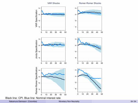
-4-2
02
0 10 20 30 40 50
VAR
Spe
cific
atio
n-4
-20
2
0 10 20 30 40 50
Jord
a Sp
ecifi
catio
n-4
-20
2
0 10 20 30 40 50Rom
er-R
omer
Spe
cific
atio
n
VAR Shocks
-4-2
02
0 10 20 30 40 50
-4
-20
2
0 10 20 30 40 50
-4
-20
2
0 10 20 30 40 50
Romer-Romer Shocks
Black line: CPI. Blue line: Nominal interest rateNakamura-Steinsson (Columbia) Monetary Non-Neutrality 64 / 64