Evaporative Heat Transfer Mechanisms within a Heat … · Evaporative Heat Transfer Mechanisms...

1

American Institute of Aeronautics and Astronautics

Evaporative Heat Transfer Mechanisms within a Heat Melt

Compactor*

Eric L. Golliher1, Daniel J. Gotti

2, Joseph E. Rymut

3, Brian K. Nguyen

4 and Jay Owens

5

NASA Glenn Research Center, Cleveland, Ohio, 44135

Greg Pace6 and John Fisher

7

NASA Ames Research Center, Moffett Field, CA

Andrew Hong8

NASA Johnson Space Center, Houston, TX

This paper will discuss the status of microgravity analysis and testing for the

development of a Heat Melt Compactor (HMC). Since fluids behave completely differently

in microgravity, the evaporation process for the HMC is expected to be different than in 1-g.

A thermal model is developed to support the design and operation of the HMC. Also, low-

gravity aircraft flight data is described to assess the point at which water may be squeezed

out of the HMC during microgravity operation. For optimum heat transfer operation of the

HMC, the compaction process should stop prior to any water exiting the HMC, but

nevertheless seek to compact as much as possible to cause high heat transfer and therefore

shorter evaporation times.

Nomenclature

k = thermal conductivity, W/m K

= conductivity of the dry trash, W/m K

= conductivity of the wet trash, W/m K

V = wall temperature minus initial temperature, K

= specific heat of the dry trash, J/kg K

= specific heat of the wet trash, J/kg K

= thermal diffusivity of the vapor and trash together, m2/s

= thermal diffusivity of the water and trash together, m2/s

= effective density of the water within a half thickness of the tile, kg/m3

L = latent heat of evaporation of water, J/kg

= temperature difference between the hot wall and the water boiling temperature, °C

t = total time to evaporate, s

X = location of the liquid/vapor front (ranges from zero at the edge to the half thickness of the tile at the

center of the tile), m

λ = intermediate numerical constant used in the analysis

1 Aerospace Engineer, Fluid Physics and Transport Branch, M. S. 77-5

2 Mechanical Design Engineer, National Center for Space Exploration Research, M.S. 110-3

3 Experimental Electrical Equipment Design Engineer, Space Combustion & Materials Branch, M. S. 110-2

4 Undergraduate Student Research Program, Fluid Physics and Transport Branch, M. S. 77-5

5 Diagnostic Research Associate, National Center for Space Exploration Research, M. S. 77-5

6 Lead Mechanical Engineer, Lockheed Martin Space Operations, 239-15

7 Technical Lead, Heat Melt Compactor Project, NASA Ames Research Center Code SCB, 239-15

8 Aerospace Engineer, Crew & Thermal Systems Branch, ES3

https://ntrs.nasa.gov/search.jsp?R=20140004924 2018-05-28T14:58:14+00:00Z

2


I. Introduction

It is imperative that we “close the loop” for human life support for future missions, and re-use as many resources

as possible. Therefore, the Logistics Reduction and Repurposing (LRR) project [1] is developing a Heat Melt

Compactor (HMC). A Heat Melt Compactor is a device that will extract residual water from astronaut’s trash (e.g.

wet wipes, juice boxes), and then compact the trash in a 10-to-1 ratio to provide easier storage, and to create “tiles”

that could provide some usefulness as an ionizing radiation shield. Since the operation of this device is gravity

dependent, consideration of microgravity operation via analysis and testing is required in order to design the

hardware. Two aspects of the process have been investigated to date: 1) the total time to evaporate the water, and 2)

the behavior of the liquid during the unheated compaction phase. The first aspect was carried out with analysis and

the second, with a low-gravity parabolic aircraft flight campaign.

There are two parts to this paper, since the degree to which we want to compact is bounded by two conflicting

goals. First, we want to compact as much as possible before heating. This minimizes the air in the tile. Air is a

very poor thermal conductor. It also minimizes the conductive path for heat transfer, which leads to greater heat

transfer into the tile and a shorter time-to-dry. The thermal model predicts the time-to-dry as a function of tile

thickness, or compaction ratio. Second, we want to compact as little as possible before heating, to minimize the

chance that liquids and solids will be squeezed out. The squeezed-out liquids or solids are undesirable, because they

would possibly foul the downstream condenser, separator, and air revitalization hardware. Squeezed out water is

potentially a serious concern in microgravity because it will tend to move with the water vapor rather than settle out.

Squeezed water is likely to contain a high level of organic and inorganic substances. Squeezed water may go where

we do not want it to go, it will breed biological growth wherever it settles, it will leave behind a residue of solids

wherever it collects and dries, and it may compromise the quality of the collected water and make the water

unsuitable for transfer to the Water Recovery System. The low-gravity flight supports the evaluation of what

compaction length minimizes or eliminates the squeezed-out water concern.

Therefore, in this paper, we summarize both the microgravity analysis that will allow an estimate of time-to-dry

as a function of total compaction length, as well as summarize the low-gravity flight test results that will allow us to

understand how water will be squeezed out as a function of total compaction length.

An analysis method using Thermal Desktop (Cullimore & Ring Technologies, Boulder, CO) was developed and

successfully benchmarked against analytical solutions. Thermal Desktop is one of the common commercial

software packages used in spacecraft thermal control.

The liquid behavior during the unheated compaction phase was investigated aboard the Zero Gravity

Corporation low-gravity aircraft. A multi-center team of flyers participated in an October 2012 low-gravity

campaign of the Zero-Gravity Corporation's Boeing 727. The funding for the flight was provided by the Office of

the Chief Technologist’s Flight Opportunities Program. A total of four days of flights were achieved, and over 170

parabolas of data acquired. The research investigated the role of capillary forces to restrain liquid within a complex

medium during a low-gravity compaction process. This supports the design of the Heat Melt Compactor system by

determining if water will exit the Heat Melt Compactor and foul the downstream condenser.

II. Microgravity Analysis for Use in Thermal Model

The goal of the microgravity fluids/heat transfer analysis was to develop a model to estimate the total time to

evaporate the water. Once the water is in the vapor state, the vapor recovery system will condense and recover the

water for eventual re-use aboard the spacecraft. Since water would normally pool in a one-g situation and not pool

in a microgravity environment, the evaporation mechanisms will be different, depending on 1-g operation or

microgravity operation. This paper will discuss only the evaporation of water in the compactor. The microgravity

analysis and discussion of the vapor recovery system will be the subject of a later paper.

In microgravity, the water does not drain towards the bottom of the compactor, and natural convection arising

from temperature gradient-induced buoyancy does not occur. Therefore, a reasonable assumption is that the water

will be evenly dispersed throughout the tile in a microgravity environment. In this case, the solutions developed for

the classic Stefan heat transfer problem are applicable [2]. On the other hand, for the 1-g case, several possible

scenarios could happen: pool boiling, a combination of pool boiling and evaporation, partial pooling with partial

Stefan problem-like evaporation, natural convection of the evaporating vapor, and evolution of boil-off in a circular

container known as the “secant effect” [3].

For the Generation 1 HMC unit, Pace[4] provided a water recovery versus time plot of testing performed in 1-g,

in both horizontal and vertical orientations. In both cases, it is thought that water pooled near the bottom of the

trash, lessening the effectiveness of the wall to provide heat to the water. In contrast with microgravity operation,

3


the water will not pool and therefore always be exposed to more wall surface area. If this Stefan problem model

accurately describes heat transfer with the HMC in microgravity, then the time-to-dry in microgravity should be

somewhat less than in 1-g. There is no microgravity or low-gravity platform to completely test the full HMC

evaporation process other than the International Space Station (ISS). A low-gravity aircraft can simulate only about

15 seconds of low-gravity, and a sounding rocket or suborbital rocket, only about 4 minutes.

Latent heat is the heat released or gained during phase change, when the temperature is ideally constant.

Sensible heat is the heat released or gained during temperature change of a material. Sensible heat is sometimes

called thermal capacitance. Typically, for any material, latent heat is much larger than sensible heat. The non-

dimensional number that describes this is Ste, the Stefan Number [5], and has a value of about 0.1 at HMC

conditions.

(1)

Convention states that with a Stefan number well below 1, the sensible heat can be neglected as a good

approximation in heat transfer analysis. This means that the thermal capacitance of the trash plays only a small role

in determining the time-to-dry, when compared to the amount of water in the trash. Further, on page 286 of Carslaw

& Jaeger [2], a formula for the Stefan problem that completely neglects thermal capacitance shows that the thermal

conductivity of the dry trash is important, while the conductivity of the wet trash plays no role:

(2)

It is planned for the operation of the heat melt compactor that the primary heating phase occurs after compaction,

so that the thermal conductance into the trash is as high as possible. If the free liquid is evenly distributed within the

trash, then a vapor/liquid front moves from the heated walls towards the middle of the trash tile. As the vapor/liquid

front moves away from the wall, the thermal conductance decreases, because the conductance length increases.

Therefore, as the evaporation proceeds, the rate of evaporation slows. A plot of evaporation rate versus time would

therefore show a steep slope at the beginning and a flatter slope later in the process.

Analytical Solution

For a one-dimensional problem considering both the latent heat and the sensible heat of the HMC, the formula

11.2 (25) of Carslaw & Jaeger [2] can be used:

[ (

)

]

(3)

Details of the formulation are presented in Chapter 11 of Carslaw and Jaeger [2], and in the analogous chapter

“Phase Change Problems” in Özişik [5]. The important boundary condition is that the domain is infinite in the

direction of the heat flow. This is different from that of a finite tile, which has an insulated boundary at the

midpoint, due to symmetry caused by heating from both sides. The Thermal Desktop model was created with

enough nodes to effectively simulate an infinite domain. There exists no analytical solution for this “slab” domain,

which would have corresponded to the tile [2]. Therefore, the Thermal Desktop model is verified by comparing it to

a semi-infinite analytical solution. Later, to predict actual tile dry times, the model boundary condition could be

easily changed to reflect the finite thickness of the tile.

The above expression (3) is solved for using the “FindRoot” command within Mathematica (Wolfram

Research, Champaign, IL). Then, the rate of vaporization, X, (the movement of the vapor/liquid front) is found by

substituting this into the following equation (4), formula 11.2 (24) of Carslaw and Jaeger[2], and plotting X

versus t:

4


√ (4)

This formulation considers only a single constituent, such as water. For the case of the HMC, the formula (3) is

modified in Equation (5) to account for the different weight ratio (different densities) of the latent heat of water to

the specific heat of the trash plus water. Per Pace[4], there exists 30% water by weight.

[ (

)

]

(5)

Assume values of the Heat Melt Compactor derived from Pace[4] and Balasubramaniam[6]:

L= 2357620 J/kg

=333.15-293.25 = 40 K

= 1200 J/kg/K

= 393.15 – 293.15 =100 K

2.746E-07

2.746E-07

=0.20

=0.20

Thermal Desktop Solution

The computer package called Thermal Desktop was used to develop a one dimensional thermal model for the

HMC compactor. This approach can be integrated later, if needed, into an overall three dimensional Thermal

Desktop model of the HMC. This would allow a three dimensional representation of the heat flow within a real

compactor. Thermal Desktop would also allow time and temperature dependent thermophysical properties and time

and temperature dependent heater characteristics. The Thermal Desktop FUSION routine was used to model one-

dimensional evaporative heat transfer and estimate the water evaporation rate. Then, these results were compared to

an exact one-dimensional analytical solution. Normally, the FUSION routine is intended to be used with

liquid/solid phase change materials (PCM) for use in spacecraft thermal control systems. The PCM spacecraft

thermal control approach is to melt wax, or some other PCM, to absorb heat during unfavorable thermal

environments, and then to freeze the PCM to release the heat later during more favorable thermal environments.

Since the FUSION routine was used in a non-standard way, it had to be verified against an analytical solution for

boundary conditions close to those that will occur with the HMC.

An approach to use PCM “nodes” was developed, analogous to thermal capacitance nodes that are typical of

lumped parameter finite difference nodes used in spacecraft thermal analysis. In this way, temperature gradients,

liquid/vapor front movement, and water recovery time histories are provided.

In Thermal Desktop, each PCM node represented a lumped parameter-type analysis of the water latent heat, as

well as non-water sensible heat portions of the trash. In order for the FUSION routine to correctly model this

evaporation process, a number of sensible heat nodes had to be inserted in between the latent heat nodes. A second

approach uses a modified temperature dependent thermal capacitance table to account for the latent heat effect. The

thermal capacitance is increased near the melting temperature, over a temperature band of 0.5 °C. Both methods

produce similar results for the HMC analysis.

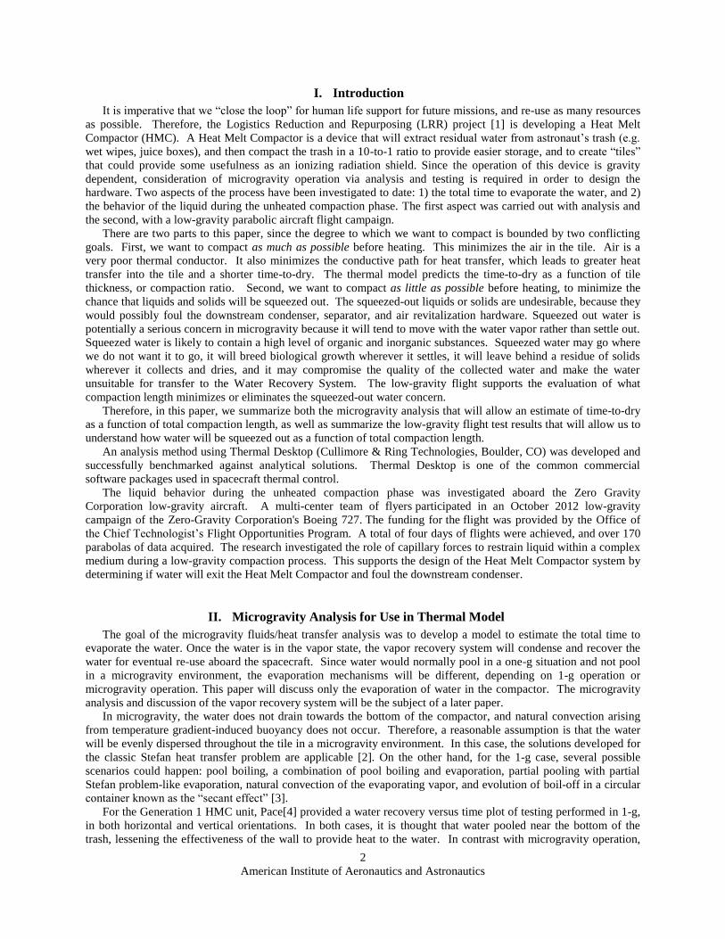
The model divided the total amount of water into 50 thermal phase change nodes, each of which represented 7.5

gm of water. Figure 1 shows the nodal layout. Per the paper from Pace[4], 150 gm of water was contained within the

500 gm of trash, and available to be recovered.

5


For most materials changing phase, the temperature of the material ideally remains constant during the phase

change process. Since this analysis uses discrete nodes to represent what is really a spatially continuous evaporation

process, the temperature versus time plots of all the nodes are “lumped” and difficult to interpret until a single

smooth plot is created by noting the endpoint of the time at which the particular node ends evaporation, and plotting

the cumulative evaporation against this endpoint time data.

The Thermal Desktop approach was compared to an exact analytical solution presented in Equations 4 and 5.

The temperature and process pressures provided by Pace[4] were used, but were standardized to 60 °C as the water

boiling point (which corresponds to a system pressure of 20 kPa) and 120 °C as the hot “wall” (piston and end cap)

temperature.

The two approaches are 1) Use the FUSION routine and 2) Modify the thermal capacitance in the thermal

properties database. The model consisted of both latent heat nodes and sensible heat nodes. The model contains 50

latent heat nodes with 5 specific heat nodes in between each latent heat node. The boundary node is held to 393.15

K. Since the distance from the surface to the first node is one half of that for the other node spacings, the first

conductor is twice the conductance value of the others.

For the FUSION routine method, each of the phase change nodes uses the following parameters:

Latent Heat= 2357620 J/kg [6]

Mass= 7.5 gm

Initial Temperature= 293.15 K

Solid Specific Heat= 1 J/kg/K

Liquid Specific Heat= 1 J/kg/K

Melting Point= 333.15 K

Each of the specific heat nodes considers the following parameters:

Initial Temperature=293.15 K

Mass= 5 gm

Specific Heat=1200 J/kg

Each of the conductors linking all the nodes:

Thermal Conductivity= 0.2 W/mK

Area/Length= 153.18 m

The first conductor linking the boundary node to the specific heat nodes and then the first latent heat node:

Thermal Conductivity= 0.2 W/mK

Area/Length= 306.36 W/mK

Model CONTROL parameters were the default except for DTIMEI, which was set to 0.01 seconds. This Thermal

Desktop parameter controls the finite difference time step and has the units of seconds. A larger DTIMEI yielded

inaccurate results.

Figure 1. Diagram Showing Arrangement of Nodes in the Thermal Model

Wall Boundary Node Dry Nodes Water Latent Heat Nodes

6


A second method does not use the FUSION routine, but instead modifies the temperature dependent thermal

capacitance such that the thermal capacitance has a step change to a higher value about the evaporation temperature

of 333 °C. If we choose a temperature interval of 0.5 °C, and divide the latent heat by 0.5, and enter this value for

the capacitance from 332.75 °C to 333.25 °C, the SINDA model can effectively account for the latent heat, without

using the FUSION routine. The real behavior is that the latent heat will not raise the temperature at all. However,

the formulation of the specific heat must assume some rise in temperature. For the purposes of this method, 0.5 °C

was considered sufficiently small. This method will work only if the temperature is steadily increasing or

decreasing, as is the case for the HMC.

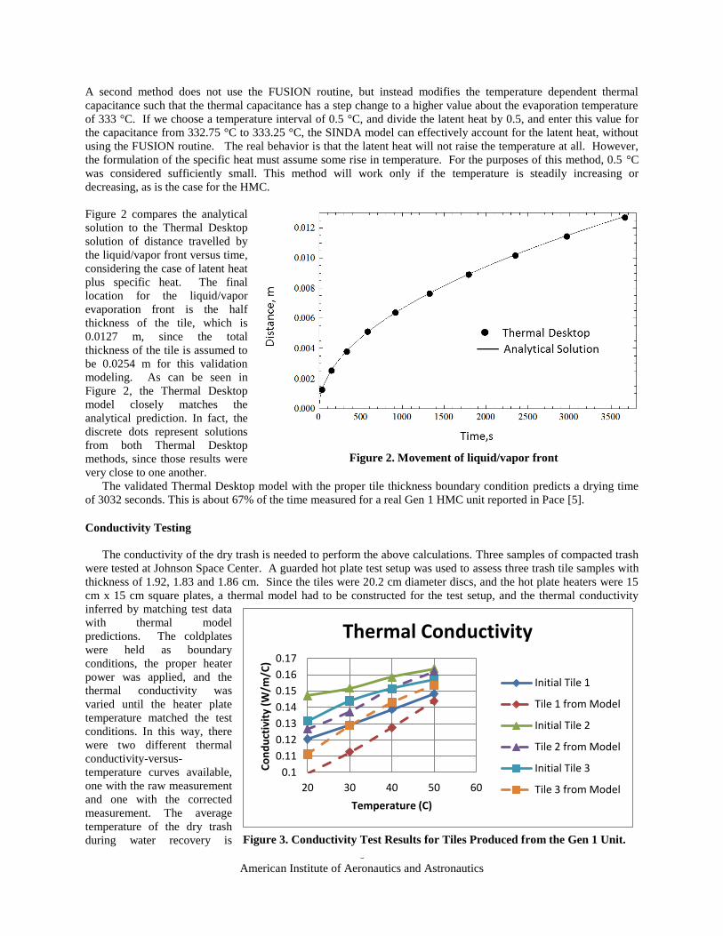
Figure 2 compares the analytical

solution to the Thermal Desktop

solution of distance travelled by

the liquid/vapor front versus time,

considering the case of latent heat

plus specific heat. The final

location for the liquid/vapor

evaporation front is the half

thickness of the tile, which is

0.0127 m, since the total

thickness of the tile is assumed to

be 0.0254 m for this validation

modeling. As can be seen in

Figure 2, the Thermal Desktop

model closely matches the

analytical prediction. In fact, the

discrete dots represent solutions

from both Thermal Desktop

methods, since those results were

very close to one another.

The validated Thermal Desktop model with the proper tile thickness boundary condition predicts a drying time

of 3032 seconds. This is about 67% of the time measured for a real Gen 1 HMC unit reported in Pace [5].

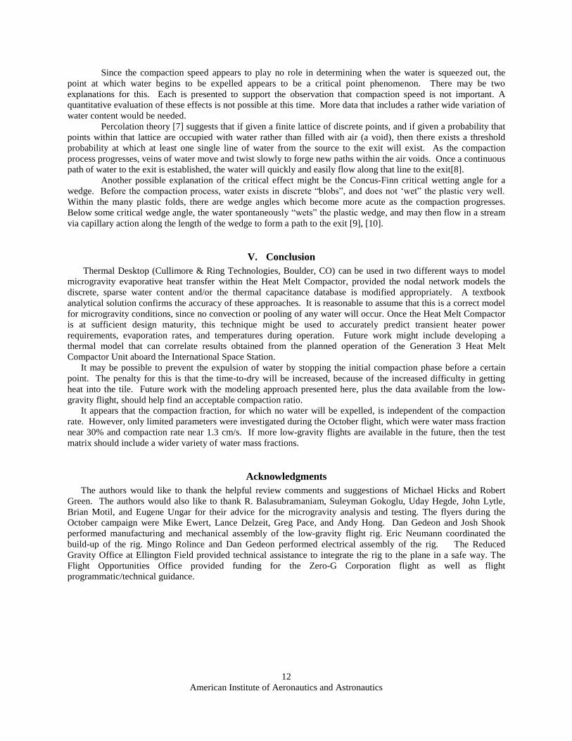
Conductivity Testing

The conductivity of the dry trash is needed to perform the above calculations. Three samples of compacted trash

were tested at Johnson Space Center. A guarded hot plate test setup was used to assess three trash tile samples with

thickness of 1.92, 1.83 and 1.86 cm. Since the tiles were 20.2 cm diameter discs, and the hot plate heaters were 15

cm x 15 cm square plates, a thermal model had to be constructed for the test setup, and the thermal conductivity

inferred by matching test data

with thermal model

predictions. The coldplates

were held as boundary

conditions, the proper heater

power was applied, and the

thermal conductivity was

varied until the heater plate

temperature matched the test

conditions. In this way, there

were two different thermal

conductivity-versus-

temperature curves available,

one with the raw measurement

and one with the corrected

measurement. The average

temperature of the dry trash

during water recovery is

0.1

0.11

0.12

0.13

0.14

0.15

0.16

0.17

20 30 40 50 60

Co

nd

uct

ivit

y (W

/m/C

)

Temperature (C)

Thermal Conductivity

Initial Tile 1

Tile 1 from Model

Initial Tile 2

Tile 2 from Model

Initial Tile 3

Tile 3 from Model

Figure 3. Conductivity Test Results for Tiles Produced from the Gen 1 Unit.

Figure 2. Movement of liquid/vapor front

7


approximately 90 °C. The curves from Figure 3 were extrapolated to 90 °C and averaged such that the estimated

thermal conductivity for use in the water evaporation modeling is 0.20 W/mK. It appears that the temperature

dependent conductivity is:

(6)

The thickness of the tiles during the conductivity testing is different than what occurred during the water

recovery portion of the process. The thickness of the tile after final compaction is less than that during the water

recovery portion of the process. Pace[4] provided a tile thickness versus time profile for the compaction process.

This is shown in Figure 4 as the “piston displacement.” The tile thickness begins at about 28 mm and ends at about

19 mm during the water recovery phase. The water recovery phase takes place in about the first 80 minutes. For the

sake of model validation, the tile thickness was assumed to be 2.54 cm.

Figure 4. Thickness of the Tile during Compaction for the Gen 1 Unit.

8


III. Low-gravity Flight Hardware

Design Considerations

A simplified version of the Gen 2 Heat

Melt Compactor was designed for use on a

low-gravity aircraft. It was designed to

meet a number of requirements in addition

to those related to compacting, resulting in

a design which looks much different than

the Gen 2 version. These requirements

include being able to view the interior of

the compactor, aircraft requirements, and

fabrication considerations.

The main parts of the aircraft version

can be seen in Figure 5. The major

differences between the aircraft version

and the Gen 2 hardware are that the aircraft

version is round in cross-section rather

than square, and it is made of cast acrylic

instead of metal. The cast acrylic was used

so that the behavior of the liquid within

could be observed, and the use of a round

cross-section allowed for much more

reliable sealing and easier fabrication. It

was determined that this shape would not

affect the liquid behavior.

The aircraft compactor and experiment

rack were also designed so that a number

of pre-packed units could be interchanged

during a test flight. This allowed multiple

tests to be conducted during a single flight.

Aircraft Compactor Description

The aircraft compactor is shown in Figure

5. It basically consists of a cylinder and a

piston, both made of cast acrylic. The cylinder is 9 in in diameter. It is closed on the top end with a cap. The bottom

is closed with the piston. They are both sealed against the cylinder with O-rings.

In order that the movement of water inside a trash compactor could be seen, clear acrylic test sections were

fabricated by the machine shop at Ames Research Center, and shipped to Glenn Research Center for integration into

the overall experiment. The diameter of the cylinder is the same as the width and depth of the Gen 2 version (9 in).

Both versions also have a piston stroke of approximately 10 in and a compaction force of approximately 3000 lb. In

addition, the air and liquid leave the aircraft compactor in a direction perpendicular to the compaction direction,

through a circumferential gap in the end cap. This gap leads to an annulus in the cap, with a single outlet port.

An exit tube is attached to this outlet port to capture any liquid that may be forced out of the compactor. The tube

is a ½ in pipe made of clear plastic. It has four holes along its length that are covered with a hydrophobic membrane

which allows air to pass through, but not water. This ensures that no pressure builds up in the compactor, and that no

water leaks out.

Aircraft Compactor Frame Description

The aircraft compactor is held within a rectangular frame which has a jackscrew mounted at the bottom. This

frame restrains the aircraft compactor while compaction is taking place. To insert the compactor into the frame, a

quick-release pin is removed and the top member of the frame is swung open. The aircraft compactor can then be

screwed onto a threaded stud located on the end of the jackscrew. The top member is then closed and fastened. A

power drill is attached to the jackscrew’s input shaft. When it is operated, the jackscrew extends, pushing the

Figure 5. Aircraft Experiment Rack. The aircraft experiment

rack installed in the Zero Gravity Corp. Boeing 727.

9


compactor’s piston upward and compacting the trash. Reversing the drill retracts the jackscrew back to its starting

position.

The aircraft compactor is contained within a secondary container. This is a rectangular box made of

polycarbonate sides, and an aluminum top and bottom. This is intended to capture any liquid that may

unintentionally escape from a compactor.

Experiment Rack Description

The compactor frame, and other

ancillary equipment, is held within

the experiment rack. The overall

experiment rack assembly is shown

in Figure 6 and Figure 7. The rack

itself is an aluminum frame of a

design that has been used for a

number of low-gravity aircraft

experiments. The compactor frame

is attached to several structural

members that are bolted to the rack.

Several other items are also

attached to the rack, such as lights

and a power strip, although these

are not shown in the drawing.

The compactor frame is

attached to the experiment rack in

such a manner that allows it to be

inverted. This allows for tests to be

conducted with some of the liquid

located at the exit of the compactor

when the test starts.

The video cameras can be seen

in the side view of the drawing.

They are used to record the

compaction events. Three cameras

provide three different views. The

first is an overall view of one side

of the aircraft compactor. The

second and third views are close-up

views of the annulus through which

the liquid exits the compactor.

These cameras are attached to

brackets which are in turn attached

to the compactor frame. This allows

the cameras to rotate with the

compactor when it is inverted,

keeping the views the same.

The jack screw used to compact the

test section was driven by a

standard commercial off the shelf power drill which was coupled to the input shaft of the jack screw. The power

drill used was a 3/8” Ryobi variable speed drill, part number D47CK (Home Depot, Brooklyn, OH). The

experiment required the power drill to turn at various different fixed speeds, however the variable speed function of

the drill could not be used because there was no way to repeatedly achieve the same consistent speed with the finger

control on the drill. After studying different options available it was determined that a low cost router speed

controller could be used to repeatedly control the speed of the drill’s brushed AC motor, which is similar to the

motor in many small routers used in wood working. The router speed controller used for this experiment was

purchased from MLCS, item number 9410 (MLCS, Huntington Valley, PA). For this experiment the speed

controller was connected to the plane’s AC power source, the drill was plugged into the speed controller, and the

Figure 6. Aircraft Compactor Assembly. Front view of the parts which

make up the aircraft compactor assembly.

10


drills finger control was fixed to the full on position so that the toggle switch on the speed controller would turn the

drill on and off while the speed control potentiometer on the controller would be used to set the speed of the drill. In

using this configuration it was found that the drill would operate with a consistent repeatable speed to turn the jack

screw. The compactors are stored in a stowage container which has been bolted to the aircraft floor next to the rack.

The container holds six compactors. Compactors which have been tested are removed from the compactor frame and

placed into the stowage container. This is usually done during a level portion of the flight.

The illumination of the test section was accomplished by a dedicated system of Light Emitting Diode (LED)

strips positioned in the corners of the frame at both top and bottom of the rack. During the rig design process,

several iterations of lighting were performed in order to ensure the cameras were able to detect water movement

inside the test section. The LED strips were White Rigid LED strips (The LED Light, Inc., Carson City, NV).

The cameras were HD Handicams (Sony, Inc.), model HDR-CX260V, equipped with 64 GB removable memory.

The AVC HD recording speed was set to the highest quality possible setting of 1920 X 1080 at 60p. The large

capacity storage cards enabled the convenience of operation as the cameras could be started before takeoff and

shutoff after landing, thereby avoiding the possible user errors of accidentally forgetting to restart a camera if the

procedure had called for stopping the camera during times when nothing was happening. The recorded video data

files were processed using Vegas Pro 11.0 (Sony, Inc.) software, at GRC’s in-house multi-user video data analysis

workstation capability. This workstation and associated software was used to evaluate, frame-by-frame, the

movement of water within the experiment.

There were three cameras on the rig: two viewed the top portion of the test section to detect when water exited

the trash, and one viewed the overall test section. These cameras were integrated into the rig and not moveable. A

hand-held fourth survey camera was available by the users to note any interesting events during the flight.

The plastic bags used in the test sections were Reclosable Sandwich Bags made of low density polyethylene,

16.5 cm X 14.9 cm, item number 415440 (Gordon Food Service, North Olmsted, OH). Nominally, a total of 350 gm

of bags and 150 gm of water were used for each trial.

Figure 7. Experiment Rack Assembly. Front and side views of the main parts of the experiment rack assembly.

11


IV. Flight Results and Discussion

The flight campaign on the Zero- g corporation’s low-gravity aircraft Boeing 727 occurred in October 2012.

The objectives of the testing were to observe how the water moves within a complex medium when the surrounding

volume is being decreased. The goals were to understand the effect of the compaction rate, the amount of water, the

effect of randomness in the results. From Pace[4], the total weight of trash was 500 gm of which 350 gm was waste

and 150 gm was water. For the low-gravity flight, plastic bags were chosen to simulate the trash. As the compaction

process occurred, the water would be forced to the edge of the top plate, where a small gap provided an entrance to a

square circular annulus and then a path to a downtube for final containment. Two HD video cameras provided a

view on both sides of the test cell near the point of compaction, and a third provided an overall view of the entire

cell. The compaction process was begun at the start of the low-g portion of the parabola and lasted about 15

seconds. The video data captured the entire compaction process and marked the point where water was first

expelled. For operator simplicity, the compaction process continued well beyond the point of first water expulsion

when the torque from the drill stalled and would drive the piston no further.

The first parameter measured was the compaction distance (cm) at which the water began to expel through the

top of the HMC piston while under compression, measured from the bottom face of the “CAP” to the compaction

“PISTON” top face (see Figure 6). The second parameter measured was the speed (cm/s) of the compaction. These

parameters were measured using the video data provided from the three video cameras and the video analysis

software called Vegas Pro 11.0 (Sony, Inc.), which was existing software installed on a workstation available to the

HMC project.

Table 1. Data showing the effect of compaction speed.

Test Cell Distance (cm) Speed/Velocity (cm/s)

Flight # 1 Tuesday Afternoon #1 3.4 1.3




Flight # 2 Wednesday Morning #1 3.1 1.2





The flight campaign consisted of 4 flights within 3 days. Each flight accomplished at least 40 parabolas. The

compaction process was performed during the 0-g parabolas. The test cell change-out process took place during the

level-flight portions of the flight. The first two flights were intended to examine the effect of compaction speed on

the amount of squeezed-out water. The second flight was a duplicate of the first, with different flight crews on each

flight, in order to test repeatability. The first flight completed testing of 4 test cells and the second flight completed

testing of 5 test cells. Table 1 shows the test results for each test cell, the distance from the end cap at which water

first was expelled, and the corresponding piston speed of compaction. As can be seen in Table 1, both flight crews

achieved nearly the same data. The reading error of the compaction length was about 0.2 cm. The standard

deviation of compaction length, considering all trials, was 1.2 cm on Flight # 1 and 1.0 cm on Flight # 2. The small

standard deviation indicates that even though the water was dispersed into the test section in a rather random and

unscientific way, and even though two different crews on two different days performed the testing, this did not lead

to a large variation in results. There was initially the assumption that the compaction rate might affect the point at

which water begins to be expelled from the chamber: a faster compaction rate would create large inertia to cause

water to exit earlier than a slow compaction rate. However, there was no statistically significant difference between

the results for the fast and slow compaction speed.

12


Since the compaction speed appears to play no role in determining when the water is squeezed out, the

point at which water begins to be expelled appears to be a critical point phenomenon. There may be two

explanations for this. Each is presented to support the observation that compaction speed is not important. A

quantitative evaluation of these effects is not possible at this time. More data that includes a rather wide variation of

water content would be needed.

Percolation theory [7] suggests that if given a finite lattice of discrete points, and if given a probability that

points within that lattice are occupied with water rather than filled with air (a void), then there exists a threshold

probability at which at least one single line of water from the source to the exit will exist. As the compaction

process progresses, veins of water move and twist slowly to forge new paths within the air voids. Once a continuous

path of water to the exit is established, the water will quickly and easily flow along that line to the exit[8].

Another possible explanation of the critical effect might be the Concus-Finn critical wetting angle for a

wedge. Before the compaction process, water exists in discrete “blobs”, and does not ‘wet” the plastic very well.

Within the many plastic folds, there are wedge angles which become more acute as the compaction progresses.

Below some critical wedge angle, the water spontaneously “wets” the plastic wedge, and may then flow in a stream

via capillary action along the length of the wedge to form a path to the exit [9], [10].

V. Conclusion

Thermal Desktop (Cullimore & Ring Technologies, Boulder, CO) can be used in two different ways to model

microgravity evaporative heat transfer within the Heat Melt Compactor, provided the nodal network models the

discrete, sparse water content and/or the thermal capacitance database is modified appropriately. A textbook

analytical solution confirms the accuracy of these approaches. It is reasonable to assume that this is a correct model

for microgravity conditions, since no convection or pooling of any water will occur. Once the Heat Melt Compactor

is at sufficient design maturity, this technique might be used to accurately predict transient heater power

requirements, evaporation rates, and temperatures during operation. Future work might include developing a

thermal model that can correlate results obtained from the planned operation of the Generation 3 Heat Melt

Compactor Unit aboard the International Space Station.

It may be possible to prevent the expulsion of water by stopping the initial compaction phase before a certain

point. The penalty for this is that the time-to-dry will be increased, because of the increased difficulty in getting

heat into the tile. Future work with the modeling approach presented here, plus the data available from the low-

gravity flight, should help find an acceptable compaction ratio.

It appears that the compaction fraction, for which no water will be expelled, is independent of the compaction

rate. However, only limited parameters were investigated during the October flight, which were water mass fraction

near 30% and compaction rate near 1.3 cm/s. If more low-gravity flights are available in the future, then the test

matrix should include a wider variety of water mass fractions.

Acknowledgments

The authors would like to thank the helpful review comments and suggestions of Michael Hicks and Robert

Green. The authors would also like to thank R. Balasubramaniam, Suleyman Gokoglu, Uday Hegde, John Lytle,

Brian Motil, and Eugene Ungar for their advice for the microgravity analysis and testing. The flyers during the

October campaign were Mike Ewert, Lance Delzeit, Greg Pace, and Andy Hong. Dan Gedeon and Josh Shook

performed manufacturing and mechanical assembly of the low-gravity flight rig. Eric Neumann coordinated the

build-up of the rig. Mingo Rolince and Dan Gedeon performed electrical assembly of the rig. The Reduced

Gravity Office at Ellington Field provided technical assistance to integrate the rig to the plane in a safe way. The

Flight Opportunities Office provided funding for the Zero-G Corporation flight as well as flight

programmatic/technical guidance.

13


References

1. Broyan, J.L. and M.K. Ewert. Logistics Reduction and Repurposing Beyond Low Earth Orbit. in International

Conference on Environmental Systems. 2012. San Diego, CA: AIAA. 20120007405

2. Carslaw, H.S. and J.C. Jaeger, Conduction of Heat in Solids Second Edition, ed. O.S. Publications. 1959: Oxford Press.

3. Ungar, E., personal communication. March 2012.

4. Pace, G., J. Fisher, L. Delzeit, R. Alba, and A. Polansky. Development of a Plastic Melt Waste Compactor for Human

Exploration Missions - A Progress Report AIAA 2010-6010. in International Conference on Environmental Systems

(ICES). 2010. Barcelona, Spain: American Institute for Aeronautics and Astronautics (AIAA).

5. Özişik, N., Heat Conduction. 1980.

6. Balasubramaniam, R., U. Hegde, and S. Gokoglu. Analysis of Water Recovery Rate form the Heat Melt Compactor. in

International Conference on Environmental Systems (ICES). 2013. Vail, Colorado: American Institute of Astronautics

and Aeronautics (AIAA), submitted for publication.

7. Balasubramaniam, R., personal communication. October 2012.

8. Medici, E.F. and J.S. Allen, Scaling percolation in thin porous layers. Physcs of Fluids, 2011. 23(122107).

9. Concus, P. and R. Finn, On the behavior of a capillary surface in a wedge. Proceedings of the National Academy of

Sciences, 1969. 63(2): p. 292-299.

10. Allen, J.S., Capillary-Driven Flow in Liquid Filaments Connecting Orthogonal Channels. 2003, Banff International

Research Station: Banff, Canada

* Trade names and trademarks are used in this report for identification purposes only. Their usage does not

constitute an official endorsement, either expressed or implied, by the National Aeronautics and Space

Administration

Evaporative Heat Transfer Mechanisms within a Heat … · Evaporative Heat Transfer Mechanisms...

Documents

Transcript of Evaporative Heat Transfer Mechanisms within a Heat … · Evaporative Heat Transfer Mechanisms...