EVAN-Toolbox IntroductoryManual...

Manuals for the EVAN Toolbox1

No. 2 V1.8 ‐ December 2012

Gerhard W. Weber and Fred L. Bookstein University of Vienna

An introduction to analysis and visualisation

1. Generalised Procrustes Analysis (GPA) ____________________________ 5 2. Principal Component Analysis (PCA) _____________________________ 10 3. Group mean difference as a deformation _________________________ 15 4. Principal Component Analysis (PCA) with different species __________ 18 5. PCA within group ____________________________________________ 20 6. Regression __________________________________________________ 23 7. Reflected relabelling for a single specimen _______________________ 26 8. Reflected relabelling for many specimens ________________________ 28 9. Partial Least Squares (PLS) _____________________________________ 30 10. Analysis of Asymmetry _______________________________________ 33

The EVAN Toolbox is software designed by Roger Phillips of the University of Hull, Paul O'Higgins of the University of York, and William D. K. Green and Fred Bookstein of the University of Vienna. Its principal systems programmers were Helgi Gunnarsson, Ramy Gowigati, Youssef Shady George‐Nashed, Vincent Dalge, and Oualid Ben Ali.

1 The EVAN Toolbox software and all the manuals in this series are distributed by the EVAN Society

EVAN‐Society, c/o Dept of Anthropology, University of Vienna, Althanstr. 14, A‐1090 Vienna, Austria evan‐[email protected] www.evan‐society.org

EVAN Toolbox - Introductory Manual 2

Our demonstrations herein refer to the April 2012 version of the EVAN Toolbox 1.51 (r1640) and the human and ape exercise data sets provided by the EVAN‐Society website (www.evan‐society.org) or the Online Material of textbook (Weber GW, and Bookstein FL. 2011. Virtual Anthropology ‐ A Guide to a New Interdisciplinary Field. Wien, New York: Springer Verlag. ISBN 978‐3‐211‐48647‐4).

Introduction The EVAN Toolbox (ET) is a software package developed by the European Virtual Anthropology Network ‐ EVAN (www.evan.at) and the EVAN‐Society to facilitate form and shape analysis of objects featuring a complex geometry. It uses Geometric Morphometrics (GM) which includes methods such as General Procrustes Analysis, Principal Component Analysis, Thin‐Plate Spline Warping or Partial Least Squares Analysis. The software also supports data acquisition, i.e. to locate landmarks and semilandmarks on surfaces and curves. The EVAN Toolbox is intended for research and education purposes. If you use ET for your work, please don't forget to acknowledge the EVAN Toolbox in the appropriate section of your publication. It is available for the systems Windows XP and Windows 7, Linux, and MacOS X. The idea behind the EVAN Toolbox is to make your life easier if your task is to analyse 3D shape and form of complexly shaped objects as we find them, for instance, in biology and medicine. ET is particularly focused on the advanced visualisation of shape and form comparisons. The application of GM procedures underlying such studies was quite demanding in terms of programming and mathematical knowledge in the past. Not every biologist, palaeontologist or medical doctor feels comfortable to code algorithms in programming languages like C++ or R. The EVAN Toolbox is built to allow those users the application of state‐of‐the‐art tools. This does, however, not save the user from studying some background how these methods are working. We tried to design ET for a broad range of users. Some standard flows for research are pre‐compiled in our collection of "Virtual Programming Networks ‐ VPNs" that are the topic of this introductory manual. The advanced user has the possibility to design own networks or to interact with our "R" node that gives the freedom to program and use whatever is needed else within the framework of ET. We are also hoping that users will add to our collection of VPNs and R routines in the future. ET was built for the demands of 3D shape and form analysis. Some of its algorithms (like the thin‐plate spline) are not adapted for use with 2D data.

About this manual This is a manual of exercises to familiarise yourself with part of the EVAN Toolbox that we assume you already have running on your desktop or laptop machine. The notes do not explain how to obtain an executable version of ET, how to launch it on your system, or how to find the main window, the VPN window, on which our attention is concentrated. For all of these matters, you will need to consult the website www.evan‐society.org and follow the procedures for registration and download there. The EVAN Toolbox divides the dataflow of a Geometric Morphometrics (GM) analysis into three general phases:

1) creation of landmark or semilandmark data, 2) analysis, and 3) viewing.

This manual does not deal with the first phase, the creation of morphometric data (but see the EVAN‐Toolbox_TemplandManual_V2.0); these demonstrations import prestructured data resources as landmark sets that already reside on surfaces that are likewise already supplied. Nor do we teach how to build workflow networks “from scratch,” starting from a blank screen. Instead, we have given you about examples of completed work flows (VPNs). The following notes combine explanations of how they are actually flowing with occasional suggestions for how to change them to do things slightly differently.


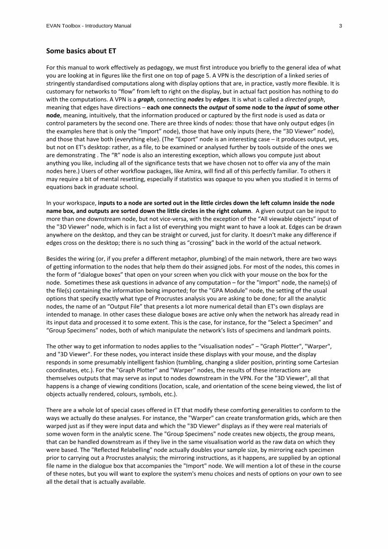
Some basics about ET For this manual to work effectively as pedagogy, we must first introduce you briefly to the general idea of what you are looking at in figures like the first one on top of page 5. A VPN is the description of a linked series of stringently standardised computations along with display options that are, in practice, vastly more flexible. It is customary for networks to “flow” from left to right on the display, but in actual fact position has nothing to do with the computations. A VPN is a graph, connecting nodes by edges. It is what is called a directed graph, meaning that edges have directions ‒ each one connects the output of some node to the input of some other node, meaning, intuitively, that the information produced or captured by the first node is used as data or control parameters by the second one. There are three kinds of nodes: those that have only output edges (in the examples here that is only the “Import” node), those that have only inputs (here, the “3D Viewer” node), and those that have both (everything else). (The “Export” node is an interesting case – it produces output, yes, but not on ET's desktop: rather, as a file, to be examined or analysed further by tools outside of the ones we are demonstrating . The “R” node is also an interesting exception, which allows you compute just about anything you like, including all of the significance tests that we have chosen not to offer via any of the main nodes here.) Users of other workflow packages, like Amira, will find all of this perfectly familiar. To others it may require a bit of mental resetting, especially if statistics was opaque to you when you studied it in terms of equations back in graduate school. In your workspace, inputs to a node are sorted out in the little circles down the left column inside the node name box, and outputs are sorted down the little circles in the right column. A given output can be input to more than one downstream node, but not vice‐versa, with the exception of the “All viewable objects” input of the "3D Viewer" node, which is in fact a list of everything you might want to have a look at. Edges can be drawn anywhere on the desktop, and they can be straight or curved, just for clarity. It doesn't make any difference if edges cross on the desktop; there is no such thing as “crossing” back in the world of the actual network. Besides the wiring (or, if you prefer a different metaphor, plumbing) of the main network, there are two ways of getting information to the nodes that help them do their assigned jobs. For most of the nodes, this comes in the form of “dialogue boxes” that open on your screen when you click with your mouse on the box for the node. Sometimes these ask questions in advance of any computation – for the "Import" node, the name(s) of the file(s) containing the information being imported; for the "GPA Module" node, the setting of the usual options that specify exactly what type of Procrustes analysis you are asking to be done; for all the analytic nodes, the name of an “Output File” that presents a lot more numerical detail than ET's own displays are intended to manage. In other cases these dialogue boxes are active only when the network has already read in its input data and processed it to some extent. This is the case, for instance, for the “Select a Specimen” and “Group Specimens” nodes, both of which manipulate the network's lists of specimens and landmark points. The other way to get information to nodes applies to the “visualisation nodes” ‒ "Graph Plotter", "Warper", and "3D Viewer". For these nodes, you interact inside these displays with your mouse, and the display responds in some presumably intelligent fashion (tumbling, changing a slider position, printing some Cartesian coordinates, etc.). For the "Graph Plotter" and "Warper" nodes, the results of these interactions are themselves outputs that may serve as input to nodes downstream in the VPN. For the "3D Viewer", all that happens is a change of viewing conditions (location, scale, and orientation of the scene being viewed, the list of objects actually rendered, colours, symbols, etc.). There are a whole lot of special cases offered in ET that modify these comforting generalities to conform to the ways we actually do these analyses. For instance, the "Warper" can create transformation grids, which are then warped just as if they were input data and which the "3D Viewer" displays as if they were real materials of some woven form in the analytic scene. The "Group Specimens" node creates new objects, the group means, that can be handled downstream as if they live in the same visualisation world as the raw data on which they were based. The "Reflected Relabelling" node actually doubles your sample size, by mirroring each specimen prior to carrying out a Procrustes analysis; the mirroring instructions, as it happens, are supplied by an optional file name in the dialogue box that accompanies the "Import" node. We will mention a lot of these in the course of these notes, but you will want to explore the system's menu choices and nests of options on your own to see all the detail that is actually available.


One last point. We have already mentioned that there are two kinds of interaction with nodes, one when the network is “running” and one before. This comes under the control of one big button at the right in the top

menu bar, the button that toggles between "Run" and "Pause" . The button is set to read the

effect of pressing it, which is the opposite of the state the network is in. If the button reads , for

instance, it means “pressing me is a pause,” thus, “the network is running”; if the button reads , it means “pressing me runs the network,” thus, “the network is not running.” If you are changing anything about the actual wiring diagram of the network – adding or deleting nodes, adding or deleting edges – you have to be in pause mode. We will proceed on the following pages with a survey of the demonstration VPNs we've supplied you. We would suggest running these on our demo data sets, thoroughly explore all the optional controls and displays, and only then run them on your own data sets instead of ours, just by changing the file names in the "Import" dialogue box. What is more important is that you are also free to build new networks that manage data flows differently from any of these standard approaches either in small details or in overall strategy. The great merit of our EVAN Toolbox architecture is that it supports both of these modes of analysis, the imitative and the creative. For technical problems, please contact evan‐[email protected] For suggestions and discussions, please visit the discussion board at www.evan‐society.org Production of the EVAN Toolbox and preparation of this manual were supported by Marie Curie Research Training Network EVAN (MRTN‐CT‐2005‐019564) and the EVAN‐Society. We thank Richard Kraft from Zoologische Staatssammlung München, Ottmar Kullmer from Senckenberg Museum Frankfurt, Barbara Herzig from Naturhistorisches Museum Wien, Wilhelm Firbas from Medical University Vienna, Franz Kainberger from Medical University Vienna, and Wolfgang Recheis from Medical University Innsbruck for support with the demonstration data used in our examples. Copyright by the EVAN‐Society.


1. Generalised Procrustes Analysis (GPA)

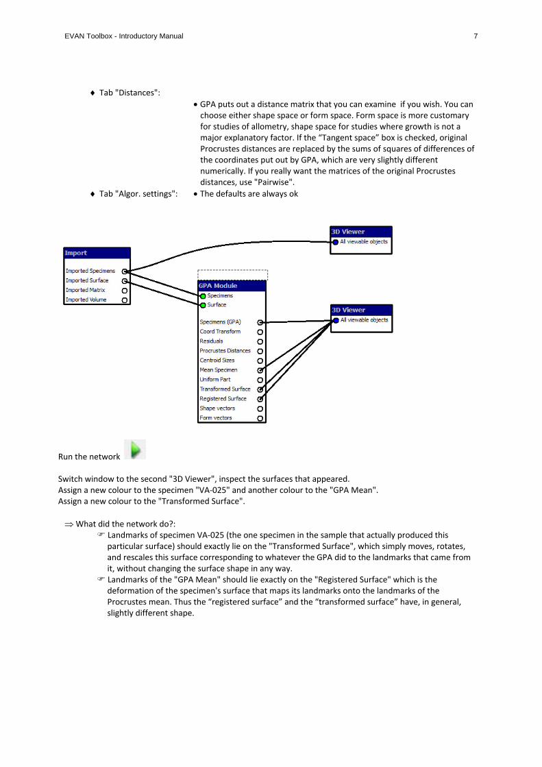
General comment: The VPN is not very complicated, so simple, in fact, that it fits on your screen (or on this page) with the data flow going almost straight from left to right, from "Import" to "3D Viewer". We are actually constructing two displays: one of the raw data points in 3D (the top "3D Viewer"), and the other of the same data after Procrustes registration (the lower "3D Viewer"). This is preferable to combining the two display lists in one viewer, as they can have arbitrarily different coordinate systems; this way, each resource gets its own origin and scale. Notice also that the “Imported Specimens” output of the "Import" node serves as input to two different nodes – to the first "3D Viewer", but also to the "GPA Module" node that in turn supplies the input to the second "3D Viewer" – and that the topmost edge on the VPN is curved simply to avoid graphical collision with the GPA box. Finally, notice that the "GPA Module" node could accept a surface as input – we will be demonstrating this below – but that it isn't required to. A surface input is optional, while a specimen input is mandatory. The surface that we are reading in isn't used yet anywhere later in the network. We will add it in as an additional resource after we have checked the basic architecture of the network as it works for just the landmarks. See below, “Modify the VPN.” Run the predefined VPN Start ET Open VPN "GPA" (menu "File" > "Open" > Specify path and filename) Double‐click node "Import"

Tab "Specimens": Choose the appropriate path and filename for "Datafile" (e.g., "VA_ExerciseDataSet_Humans.txt")

Run the network [meaning: click the button, which changes its status to “Running” and, at the same

time, changes the button to "Pause" for your next click] Double‐click the first (upper) node "3D Viewer" Double‐click the second (lower) node "3D Viewer" " Resize each until both fit on your screen. These viewers are, in principle, completely independent; neither one knows what the other one is

doing, even if they are driven by closely related display resources. Switch window to the first "3D Viewer", inspect the raw landmarks of all specimens, rotate the space with left

mouse button Switch window to the second "3D Viewer", inspect the registered landmarks of all specimens, rotate the space

with left mouse button


Assign a different colour to VA‐001: click on the specimen in the right column of its viewer with right mouse

button, change "Front Material" to new colour Make an image: click on menubar "Capture", then "Get a screenshot", specify path and filename, choose ".png",

".jpg" or "bmp" Try menubar "Stereo Mode" (pull down menu of options for stereoscopic viewing, if you have the hardware to

use one of its options such as "Quad Buffer", "Anaglyphic" or others) Go back to the main window

Pause the network [meaning: press the button, changing from “Running” to “Paused” and, at the same

time changing this button to "Run" for your next click] Modify the predefined VPN to obtain additional visualisations Double‐click node "Import"

Tab "Surface": Choose the appropriate path and filename for "Surface file" (e.g., "VA_ExerciseDataSet_Humans.stl")

Set the number of the specimen to associate this surface with (e.g. #15 for the VA_ExerciseDataSet_Humans.txt; we have chose

this one, simply because it had the nicest surface) Connect "Imported Surface" of the "Import" node with "Surface" of the "GPA Module" node, connect "Mean

Specimen", "Transformed Surface" and "Registered Surface" of the "GPA Module" node with "All viewable objects" of the second "3D Viewer" node. The difference between these two types of GPA surface output will be explained below.

Double‐click node "GPA Module" if you want to see the options or to change some of them.

Tab "Fitting options":

The defaults are appropriate for the usual GPA. The options to not translate, not rotate, or not scale are for other kinds of applications, such as gait analysis. Likewise, in Geometric Morphometric (GM) studies, the rotation of the Procrustes shape coordinates is a matter of convenience. Usually it is good enough to align “by principal axes,” meaning that the X‐axis is along the direction of greatest principal moment (sum of squares) around the centre of mass, the Y‐axis along the second principal moment, and the Z‐axis perpendicular to the XY‐plane. For an analysis of bilateral asymmetry, however, one does better to pick the last choice (align the XY‐plane with the plane of symmetry). "Tangent project coordinates" should be left checked (the default) almost always. You uncheck it if you have extremely wide shape variation and want to see the effect of the curving (non‐euclidean)geometry of Kendall's shape space.

Specify a path and filename for the "Output file" if desired


Tab "Distances":

GPA puts out a distance matrix that you can examine if you wish. You can choose either shape space or form space. Form space is more customary for studies of allometry, shape space for studies where growth is not a major explanatory factor. If the “Tangent space” box is checked, original Procrustes distances are replaced by the sums of squares of differences of the coordinates put out by GPA, which are very slightly different numerically. If you really want the matrices of the original Procrustes distances, use "Pairwise".

Tab "Algor. settings": The defaults are always ok

Run the network Switch window to the second "3D Viewer", inspect the surfaces that appeared. Assign a new colour to the specimen "VA‐025" and another colour to the "GPA Mean". Assign a new colour to the "Transformed Surface".

What did the network do?: Landmarks of specimen VA‐025 (the one specimen in the sample that actually produced this

particular surface) should exactly lie on the "Transformed Surface", which simply moves, rotates, and rescales this surface corresponding to whatever the GPA did to the landmarks that came from it, without changing the surface shape in any way.

Landmarks of the "GPA Mean" should lie exactly on the "Registered Surface" which is the deformation of the specimen's surface that maps its landmarks onto the landmarks of the Procrustes mean. Thus the “registered surface” and the “transformed surface” have, in general, slightly different shape.


Open the output file with an editor. You will find a summary of: the number of individuals, landmarks, and dimensions,

the coordinates of the Procrustes mean shape [centred at (0,0,0), scaled to Centroid Size = 1] and in the orientation specified in a previous dialogue box

the Procrustes distances between specimens, and the Centroid Sizes (CS) and their natural logarithms (lnCS) To obtain the Procrustes coordinates for each specimen:

Go back to the main window

Pause the network Get a new "Export" node and place it anywhere on the workspace (in the left hand menu of ET's main

window click on the "Data" tab, then on the node "Export", move your mouse over the workspace and click, the new node will be dropped there),

Connect the "Specimens (GPA)" output of the "GPA Module" node to the "Specimens" input of the "Export" node, and connect "Shape vectors" of the "GPA Module" node with "Data Matrix" of the "Export" node

Run the network Double‐click "Export" node

Tab "Specimens": Choose appropriate format (e.g., .xls) and check "Include Labels"

Click "Export Specimens", specify path and filename

View the exported file that contains the Procrustes shape coordinates in decimal form Try the same with "Form vectors" instead of "Shape vectors" (but before you do this, switch to

"Form Space Distances" in the tab "Distances" in the "GPA Module" node)


You might want to export these typed shape coordinates if, for instance, you want to know the total Procrustes variation in a data set, but you do not want to use our regression node to get it.

Closing note: Here at the end of our first example, you've already seen prototypes of many of the ways you interact with a network in general. We have demonstrated the examination of standard views (raw coordinates, shape coordinates), the enhancement of these views by surface imagery, and then the comparison of two different ways of visualising by direct superposition in the same viewing window (the picture with both of the surfaces from GPA, the “transformed” and the “registered” shown atop one another). We have also shown how you stop the network, change it, and start it again. There will be many more examples of all these interactive strategies in the other VPNs to follow.


2. Principal Component Analysis (PCA)

General comment: One of the outputs of the PCA, the PC scores, is sent to two different inputs of another node, the "Graph Plotter". The "Warper" produces three outputs, new landmark locations, new surface forms, and new (warped) grids, all of which are input to the "3D Viewer" node (within which the user chooses which of them are to be made visible at a given time). Of the three main outputs of the "PCA" node, two (the scores and the eigenvectors) go on down the network as inputs to the plotter, while the third, the eigenvalues, is simply ignored (unless you've asked for an output file, in which case they are printed there). The long edges from "GPA Module" over to the "Warper" are the network's way of passing the information that the warper needs to decide what is actually being warped – here, the landmarks start at the GPA mean, and the surface warp likewise starts from the surface supplied by the "Import" node but subsequently deformed so as to match those mean landmark positions. These edges make explicit what is often puzzling to the person who is trying to program the same displays in a lower‐level context such as "R". The edges connecting the "Graph Plotter" node to the "Warper" node, likewise, stand for the expression of the scientist's intention that is otherwise somewhat difficult to program: a point on a PC plot stands for the warp that drives all landmarks away from their average positions along the directions of the corresponding PC's, not a direction in the space of the original data. Run the predefined VPN Start ET Open VPN "PCA" Double‐click node "Import", and then, as in the previous VPN,



Set the number of the specimen to associate this surface with (e.g. #15 for the VA_ExerciseDataSet_Humans.txt) Double‐click node "GPA Module" or accept the defaults as in the previous VPN

Tab "Fitting options": Choose your settings as described above for GPA Tab "Distances": Choose your settings as described above for GPA Tab "Algor. settings": Choose your settings as described above for GPA Double‐click node "PCA" to review and accept the default options or to change some of them.

The default is to centre the columns (the "variables"), which is how GPA output always comes. The dialogue box is asking about this because PCA can take data from any matrix, not necessarily just shape coordinates, and until the network runs it can't know which of its inputs actually have mean zero and which don't. For this reason, there is an option for not centring which assumes that the value 0 of your original variables has some scientific meaning. For the same reason, we offer an option that is usually called "Z‐scoring" but that isn't used with Procrustes analysis (because


shape coordinates have to be scaled to Procrustes distance, not to variance). Scaling of eigenvectors differs from discipline to discipline; we offer both of the standard choices, but default to the option more commonly encountered in Procrustes analysis is the first option, unit length. For other kinds of variables, one usually checks the second option. The last checkbox is very important because it determines what kind of analysis you are going to get, shape space or form space. Form space is the more customary for studies of allometry, shape space for studies that do not involve a growth factor.

Specify a path and filename for the "Output file"

Run the network Manipulate the visualisations

Pause the network Double‐click the node "Graph Plotter" Enlarge the window (taking care not to lose the specimen at the upper left !) Assign different colours to human females and human males (later on we will do this with a node): click on

each with your right mouse button, change "Front material" to new colour The plot of the PC 1 vs. PC 2 shows two things: the females (in red) are generally to the upper right of the males (as in real life), but also there is an obvious outlier, VA‐051, that needs inspection: Has it, for instance, a particularly flat face and at the same time a bulging occipital region?


Click on any specimen on the right panel watch where it lights up in the plot Set bigger symbol size or change to another plot symbol for a specimen (right click in column "Size" in the right

panel, choose "Size" and change value, or change the symbol in column "Plot Symbol" to "Triangle") Add a title to the plot (menu "Plot" > "Title" > "Set Text") Set axis limits (menu "Plot" > "Axes" > "Set Axes Limits") But don't change "Square Axes" (because this plot is in Procrustes geometry which requires the same spacing on every axis) Hide the mouse coordinates (menu "Plot" > "Hide mouse coordinates") Export graph (menu "Plot" > "Export" > specify path and filename, choose filetype ".png", ".jpg", "bmp", ".svg",

".pdf", or ".ps" Change X‐axis to "PC 2" and Y‐axis to "PC 3" Go back to the main window.

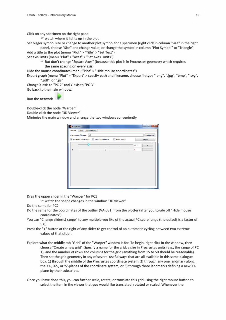
Run the network Double‐click the node "Warper" Double‐click the node "3D Viewer" Minimise the main window and arrange the two windows conveniently

Drag the upper slider in the "Warper" for PC1 watch the shape changes in the window "3D viewer" Do the same for PC2 Do the same for the coordinates of the outlier (VA‐051) from the plotter (after you toggle off “Hide mouse

coordinates”). You can "Change slider(s) range" to any multiple you like of the actual PC score range (the default is a factor of

5.0). Press the "+" button at the right of any slider to get control of an automatic cycling between two extreme

values of that slider. Explore what the middle tab "Grid" of the "Warper" window is for. To begin, right click in the window, then

choose "Create a new grid". Specify a name for the grid, a size in Procrustes units (e.g., the range of PC 1), and the number of rows and columns for the grid (anything from 15 to 50 should be reasonable). Then set the grid geometry in any of several useful ways that are all available in this same dialogue box: 1) through the middle of the Procrustes coordinate system, 2) through any one landmark along the XY‐, XZ‐, or YZ‐planes of the coordinate system, or 3) through three landmarks defining a new XY‐plane by their subscripts.

Once you have done this, you can further scale, rotate, or translate this grid using the right mouse button to

select the item in the viewer that you would like translated, rotated or scaled. Whenever the


underlying landmark configuration is warped, so will these grids be warped, along with whatever surfaces are also in the Viewer's display list.

You can also add additional grids parallel or perpendicular to any placed previously.


An interesting aspect of this network is that the "Warper" node has two modes of input that are available to you simultaneously. In one approach, you interact directly with the warper, moving its slider bars by your own hand on the mouse. In the other version of exactly the same control process, you move the mouse in the "Graph Plotter" window, and the corresponding slider bars in the Warper are slaved to the two coordinates under your mouse. But the "Warper" in this network doesn't know anything about the PCA. Notice, for instance, that its sliders do not get their input from the PCA, but are controlled by the "Graph Plotter", which has little scroll windows for assigning particular PC's to the X‐ and Y‐axes of the plot. The two screenshots above show the output for PC 1 at ‐0.13 and +0.13. See what a good idea it was to have the “Registered Surface” available for output – it warps from the same (0,0,0) configuration that the PCA assigns to the landmark mean shape itself. If you open the PCA output file, you will find a summary of the PCA in standard statistical terms, including:

the eigenvalues of the PCs and the percentages of total Procrustes variance "explained" all PC scores for all specimens all PC loadings for all shape coordinates


3. Group mean difference as a deformation

General comment: The group averages that are computed with the aid of the "Group Specimens" node being introduced here are actually used as input by three separate nodes downstream, the two different "Select a Specimen" nodes and the "Generate Surface" node that is used when a surface needs to be registered to something other than the actual GPA mean. There are now four items on the "3D Viewer" display list, three from the "Warper" and one from the "Group Specimens" node (a pass‐through of the shape coordinates from the "GPA Module" node, except that each specimen has been assigned a colour corresponding to its group assignment). The other new node here, "Subtract", is necessary to give the "Warper" a direction in shape space for its slider to slide along, as you can see because the only output of "Subtract" is this particular input to the "Warper". It Is typical of GM applications that the network design incorporates a choice of what is worth visualising: in this case, it is the effect of changes in the multiple of this vector used for the warping, not any other kind of visualisation such as an explicit display with little arrows at each landmark (the more customary printed iconography). The design of a VPN thus incorporates opinions about “best practices” within the world of GM generally, in this case ours, but other choices are certainly possible. The two different "Select" nodes are identical copies; the difference in their positions in the network flow is purely that at run time you will instruct one to select the male average shape, and the other, the female average. You will have also decided that the "Warper" will be centred on the male average and produce the female form as a deformation of it, instead of vice versa (obviously a rhetorical decision, not a scientific one). Run the predefined VPN Start ET Open VPN "GroupMeans" Double‐click node "Import" and make all the same choices as in the two previous VPNs



Set the number of the specimen to associate this surface with (e.g. #15 for the VA_ExerciseDataSet_Humans.txt) Double‐click node "GPA Module" and take or reject the default options as before

Tab "Fitting options": Choose your settings as described above for GPA Tab "Distances": Choose your settings as described above for GPA Tab "Algor. settings": Choose your settings as described above for GPA

Run the network Carry out the selection operations When you run the VPN you will recognize red dots indicating that computations could not be completed. This is

not a user error, but a signal that some nodes require run‐time interaction with you in order to proceed: in this case, you have to specify the selection rules (leave the network in run mode).


Double‐click on the "Group Specimens" node to specify the groups:

Click on "New Group" and name it "Males".

Remember that there is a variable "Sex" in the input Morphologika file.

Type "[Sex = 1]" into the empty box lower left, near the button "Add to Selection".

Click on this "Add to Selection" button (all specimens fulfilling the criterion will be marked).

Click on the ">>" button in the middle. This creates the group of specimens.

Do this again for females using the filter "[Sex = 2]".

Click on each group name to set its colours (right mouse button).

Check "Automatically Append a Group Mean" (we will be using these to drive the Warper). Click on either one of the "Select a Specimen" nodes. You will see a list of the two mean specimens. (Why only

the means? Because that's what the network sent this node as output from the "Group Specimens" node! See, in the VPN, how the specimens themselves are sent only to the "3D Viewer", not the intermediate selection operations.) Choose one or the other mean and you'll see its Procrustes mean shape coordinates in the right column. Do the same for the other one.

Notice the "Generate Surface" node, which is needed in order to get the one surface loaded (VA‐

025) from the grand mean (which is where the GPA puts it) to the male mean (which is where we want the "Warper" to start). This node will ask which of the group means is the one intended for use as the “Target” for the surface warp here.

The "Subtract" node is actually a general two vector linear combination, but we are using it here in

its default mode, which is to subtract the target from the source. Its output is therefore the vector from the mean female (1) to the mean male (0). (The generality accounts for the somewhat confusing phrasing of its operation, which is typed as documentation right there in the node's dialogue box.)

Manipulate the visualisation Open the "3D Viewer" and slide the slider of the "Warper" back and forth.

It will warp between a male (0) and a female (1), or between a hyper‐female (> 1) and a hyper‐male (< 0), as you like. The slider for the following images below were set to ‐2.0 and + 2.0.

The "Warper" now has only one slider for the one vector it was sent (this input to the "Warper" is the output of the "Subtract" node). The warper's other two inputs came from the top "Select a Specimen" node (the “Base Specimen” for the warp, the specimen at 0 warping, is the male mean) and from the "Generate Surface" node, which warped the surface acquired by the "Import" node to exactly fit the coordinates of the mean male.

Use the middle tab "Grid" of the "Warper" window and create grids as described in the "PCA" VPN.

Turn off the "Warped Surface" in the "3D Viewer" and watch the "Warped Landmarks" and the grids while moving the slider of the "Warper".


4. Principal Component Analysis (PCA) with different species

General comment: We use the "PCA" VPN from the previous section with another input file to visualise within and between species variation using the "Graph Plotter" display, as shown in the next figure below. This would actually constitute primary scientific findings if we didn't already know this and our sample sizes would be larger. Run the predefined VPN Start ET Open VPN "PCA" Double‐click node "Import" and change one of the specifications from the earlier demo's:

Tab "Specimens": Choose the appropriate path and filename for "Datafile" (e.g., "VA_ExerciseDataSet_Humans&Apes.txt")


Set the number of the specimen to associate this surface with (e.g. #15 for the VA_ExerciseDataSet_Humans.txt) Double‐click node "GPA Module"

Tab "Fitting options": Choose your settings as described above for GPA Tab "Distances": Choose your settings as described above for GPA Tab "Algor. settings": Choose your settings as described above for GPA

Double‐click node "PCA" Choose your settings as described above for PCA Specify a path and filename for the "Output file"

Run the network Interact with the network Open the "Graph Plotter" and assign different colours to humans, chimpanzees and orangutans.

View the species differences in the first two PCs and then switch to other combinations of PCs. Notice that the outlier we saw in the PCA of the humans by themselves is no longer in evidence.

The dimension along which it is outlying is not either of these principal components – the way it is outlying is not typical of the contrast with either chimpanzees or orangutans.


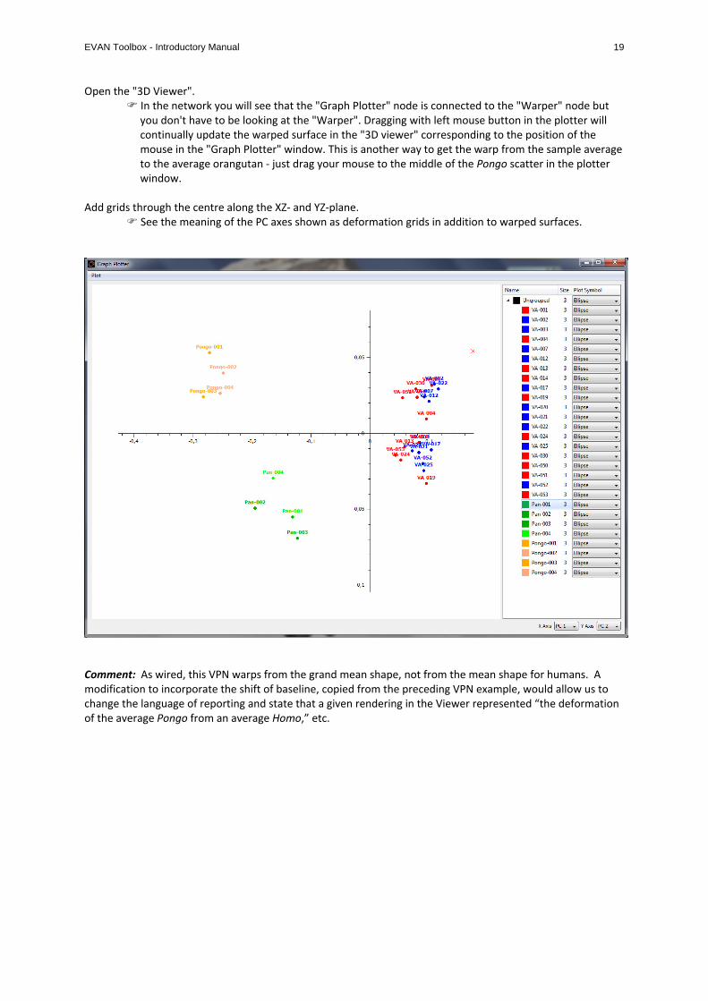
Open the "3D Viewer". In the network you will see that the "Graph Plotter" node is connected to the "Warper" node but

you don't have to be looking at the "Warper". Dragging with left mouse button in the plotter will continually update the warped surface in the "3D viewer" corresponding to the position of the mouse in the "Graph Plotter" window. This is another way to get the warp from the sample average to the average orangutan ‐ just drag your mouse to the middle of the Pongo scatter in the plotter window.

Add grids through the centre along the XZ‐ and YZ‐plane.

See the meaning of the PC axes shown as deformation grids in addition to warped surfaces.

Comment: As wired, this VPN warps from the grand mean shape, not from the mean shape for humans. A modification to incorporate the shift of baseline, copied from the preceding VPN example, would allow us to change the language of reporting and state that a given rendering in the Viewer represented “the deformation of the average Pongo from an average Homo,” etc.


5. PCA within group

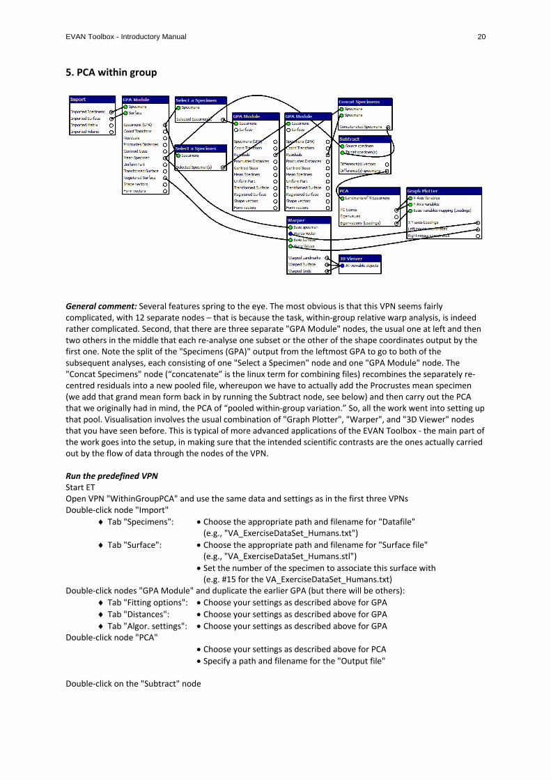
General comment: Several features spring to the eye. The most obvious is that this VPN seems fairly complicated, with 12 separate nodes – that is because the task, within‐group relative warp analysis, is indeed rather complicated. Second, that there are three separate "GPA Module" nodes, the usual one at left and then two others in the middle that each re‐analyse one subset or the other of the shape coordinates output by the first one. Note the split of the "Specimens (GPA)" output from the leftmost GPA to go to both of the subsequent analyses, each consisting of one "Select a Specimen" node and one "GPA Module" node. The "Concat Specimens" node (“concatenate” is the linux term for combining files) recombines the separately re‐centred residuals into a new pooled file, whereupon we have to actually add the Procrustes mean specimen (we add that grand mean form back in by running the Subtract node, see below) and then carry out the PCA that we originally had in mind, the PCA of “pooled within‐group variation.” So, all the work went into setting up that pool. Visualisation involves the usual combination of "Graph Plotter", "Warper", and "3D Viewer" nodes that you have seen before. This is typical of more advanced applications of the EVAN Toolbox ‐ the main part of the work goes into the setup, in making sure that the intended scientific contrasts are the ones actually carried out by the flow of data through the nodes of the VPN. Run the predefined VPN Start ET Open VPN "WithinGroupPCA" and use the same data and settings as in the first three VPNs Double‐click node "Import"



Set the number of the specimen to associate this surface with (e.g. #15 for the VA_ExerciseDataSet_Humans.txt) Double‐click nodes "GPA Module" and duplicate the earlier GPA (but there will be others):

Tab "Fitting options": Choose your settings as described above for GPA Tab "Distances": Choose your settings as described above for GPA Tab "Algor. settings": Choose your settings as described above for GPA Double‐click node "PCA"

Choose your settings as described above for PCA Specify a path and filename for the "Output file"

Double‐click on the "Subtract" node


In the “Subtract” node, the coefficients set in the dialogue box are +1.0 for A and +1.0 for B.

As the coefficients of this "Subtract" node are a function of the network design, not of the data, they do not need to be set at run time – in the case of these demo's, they were imported when you read in the VPN in the first place.

Run the network Interact with the network When you run the VPN you will recognize red dots indicating that selection of two subsets need to be done

during the run. Open each "Select a Specimen" node in turn and select one sex or the other:

Type "[Sex = 1]" into the empty box left to the button "Add to Selection"

Click on the "Add to Selection" button Click "OK" Do this again for females using the command "[Sex = 2]"

The red dots turn green and the network has now run successfully, all the way to the end (the

Graph Plotter). What did the network do?:

It created separate GPAs for the males and the females, produced residuals as if they referred to the same mean form (even though they do not), carried out an ordinary PCA of the combined data of both sets of residuals, and, finally, added the original grand mean back in. What results can be visualised by the usual "Graph Plotter" ‐ "Warper" ‐ 3D Viewer" triumvirate?

Open the "Graph Plotter", go down the list of males and change their colour.

You could see if the pattern of their covariance was different from that of the females. In this example they appear to be the same except for that one outlying female VA‐051. Because these are pooled within‐group PC's, each sex has to average (0,0) separately; this means that the outlying female, has actually shifted all of the other females in the opposite direction.

If you want to test for significant differences between these covariance structures, you want to export the PC scores from the "PCA" node to "R" or any other statistics package along with the group labels. This is the standard context for which pooled within‐group analyses are intended.

The analysis here does not look much different from the analysis in the preceding VPN because the group mean shapes differ only slightly. In other applications, for instance to differences between species or to highly sexually dimorphic species, the effect of within‐group centring would be greater.


6. Regression

General comment: A whole week of the usual course in GM is hidden in this VPN, in particular, in the one‐edge connection between an output of the "Regression" node and an input of the "Warper" node. The EVAN‐Toolbox “knows” that when we talk about regression of shape on its predictors, we mean regressing each shape coordinate separately on the selfsame list of predictors. So the relevant arrays have three subscripts, two for the landmarks (landmark number by X, Y, Z coordinate) and one for the list of predictors. The tie between the "Regression" and the "Warper" nodes understands all of this as part of its built‐in algebra, so that the single edge of the VPN graph here, from “Regression Coefficients” to “Warps Vector”, is all that the user needs to specify. We have thereby saved an amazing amount of tedium in comparison to the corresponding specification in any standard statistical package. Run the predefined VPN Start ET Open VPN "Regression" Double‐click node "Import" and set it as in .vpn's 1, 2, 3:



Set the number of the specimen to associate this surface with (e.g. #15 for the VA_ExerciseDataSet_Humans.txt) Double‐click node "GPA Module" and verify its defaults as always:

Tab "Fitting options": Choose your settings as described above for GPA Tab "Distances": Choose your settings as described above for GPA Tab "Algor. settings": Choose your settings as described above for GPA Double‐click node "Regression"

In the usual application the "Dependent variables" are the shape (or form) coordinates (with "Shape" as the default) and the "Independent variables" include 1) Centroid Size or ln Centroid Size (pick only one), and also 2) any other variables you read in from your Morphologika file (e.g., Sex). You are required to choose a sub‐list from these variables, for instance, lnCS and sex.

There is another option called "Standardise Specimens" that you use when you have non‐parallel regressions. In this case, you could use it to eliminate the regression on size in favour of an adjustment to size 1 prior to a regression that is now just on sex.

Specify a path and filename for the "Output file"


Run the network Open the output file

In the output file you will the get:

A summary of the raw data (the dependent [X1, Y1, Z1, X2, Y2, Z2, ..., Z25] and independent variables [lnCS, sex] for each case used in the regression).

Below that, there is the ususal statistic for each dependent variable (coefficients Beta[0], Beta[first independent], Beta[second independent], …, p‐values, R2 for each shape coordinate, F‐Test, p‐values, etc.

At the bottom is the summary regression statistics including Wilk’s Lambda, Pillai’s Trace, Hotelling Lawley's Trace, Roy's Largest Root, and the fraction of variance explained by the regression

It should be noted that these statistics, although common practice in many applications, are considered to be inappropriate for the kind of application we are dealing here (see e.g., Mardia et al. 2000 Biometrika 87: 285–300; Weber & Bookstein 2011, Springer Verlag)

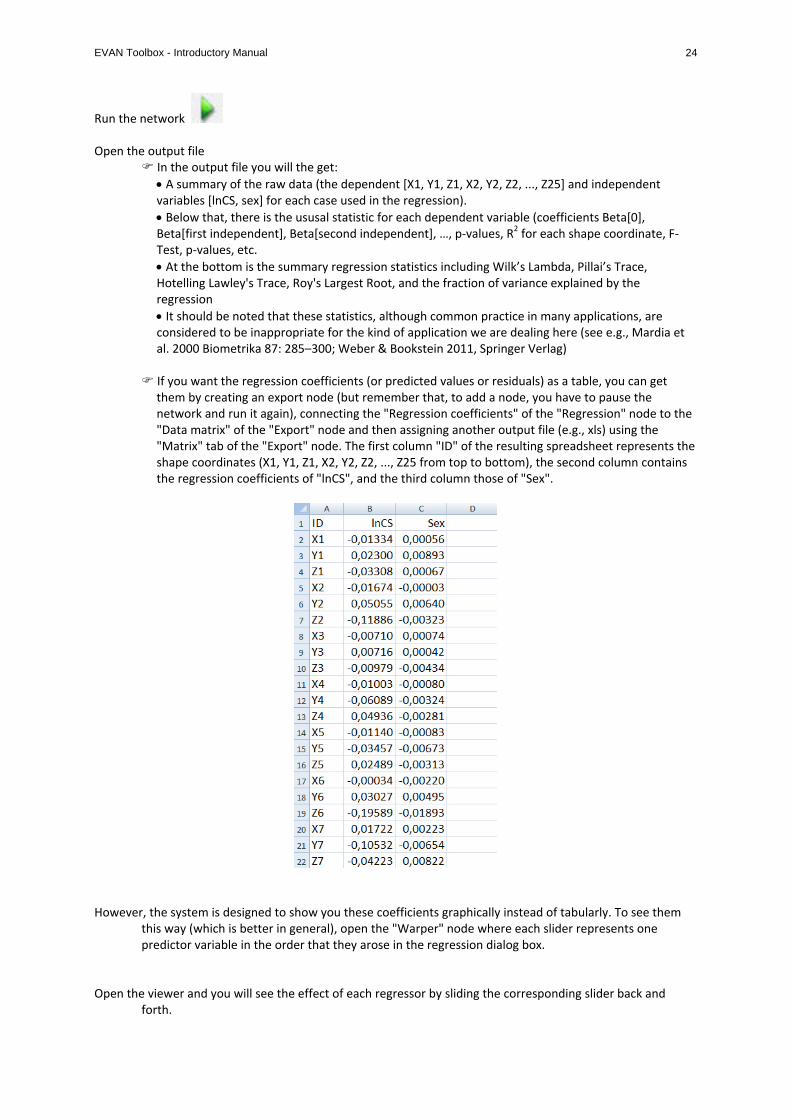
If you want the regression coefficients (or predicted values or residuals) as a table, you can get

them by creating an export node (but remember that, to add a node, you have to pause the network and run it again), connecting the "Regression coefficients" of the "Regression" node to the "Data matrix" of the "Export" node and then assigning another output file (e.g., xls) using the "Matrix" tab of the "Export" node. The first column "ID" of the resulting spreadsheet represents the shape coordinates (X1, Y1, Z1, X2, Y2, Z2, ..., Z25 from top to bottom), the second column contains the regression coefficients of "lnCS", and the third column those of "Sex".

However, the system is designed to show you these coefficients graphically instead of tabularly. To see them

this way (which is better in general), open the "Warper" node where each slider represents one predictor variable in the order that they arose in the regression dialog box.

Open the viewer and you will see the effect of each regressor by sliding the corresponding slider back and

forth.


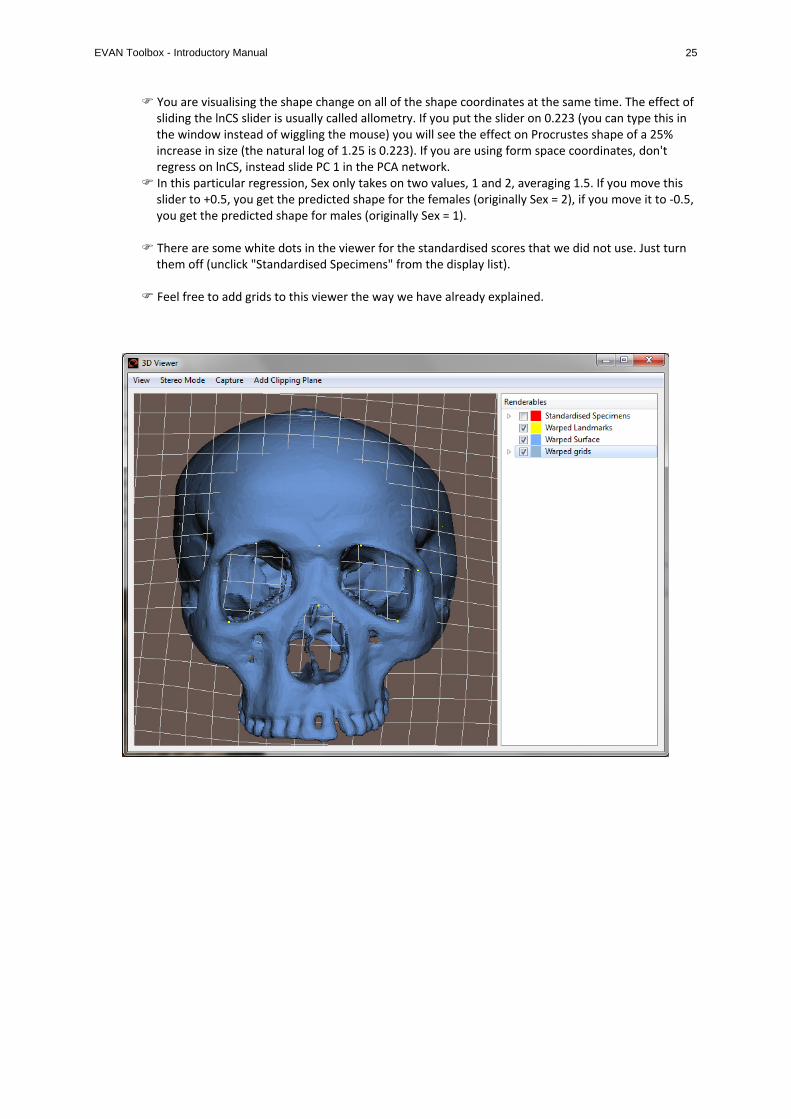
You are visualising the shape change on all of the shape coordinates at the same time. The effect of sliding the lnCS slider is usually called allometry. If you put the slider on 0.223 (you can type this in the window instead of wiggling the mouse) you will see the effect on Procrustes shape of a 25% increase in size (the natural log of 1.25 is 0.223). If you are using form space coordinates, don't regress on lnCS, instead slide PC 1 in the PCA network.

In this particular regression, Sex only takes on two values, 1 and 2, averaging 1.5. If you move this slider to +0.5, you get the predicted shape for the females (originally Sex = 2), if you move it to ‐0.5, you get the predicted shape for males (originally Sex = 1).

There are some white dots in the viewer for the standardised scores that we did not use. Just turn

them off (unclick "Standardised Specimens" from the display list). Feel free to add grids to this viewer the way we have already explained.


7. Reflected relabelling for a single specimen

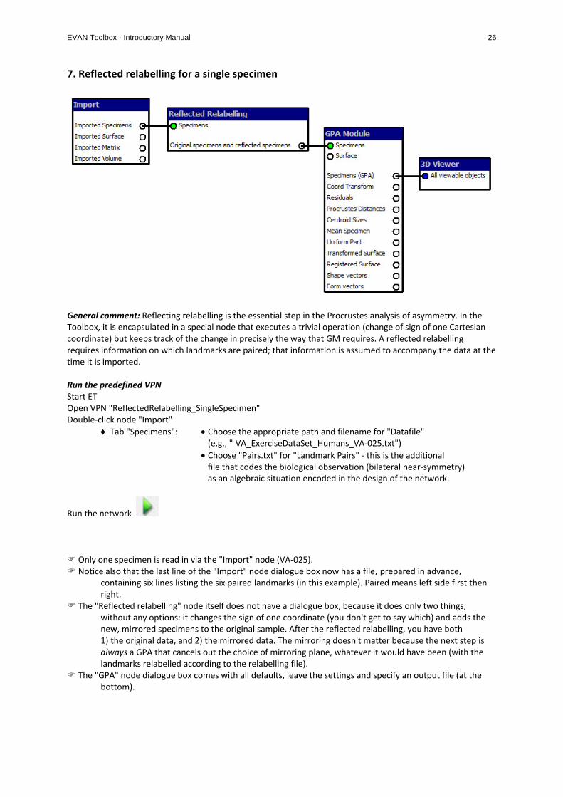
General comment: Reflecting relabelling is the essential step in the Procrustes analysis of asymmetry. In the Toolbox, it is encapsulated in a special node that executes a trivial operation (change of sign of one Cartesian coordinate) but keeps track of the change in precisely the way that GM requires. A reflected relabelling requires information on which landmarks are paired; that information is assumed to accompany the data at the time it is imported. Run the predefined VPN Start ET Open VPN "ReflectedRelabelling_SingleSpecimen" Double‐click node "Import"

Tab "Specimens": Choose the appropriate path and filename for "Datafile" (e.g., " VA_ExerciseDataSet_Humans_VA‐025.txt")

Choose "Pairs.txt" for "Landmark Pairs" ‐ this is the additional file that codes the biological observation (bilateral near‐symmetry) as an algebraic situation encoded in the design of the network.

Run the network Only one specimen is read in via the "Import" node (VA‐025). Notice also that the last line of the "Import" node dialogue box now has a file, prepared in advance,

containing six lines listing the six paired landmarks (in this example). Paired means left side first then right.

The "Reflected relabelling" node itself does not have a dialogue box, because it does only two things, without any options: it changes the sign of one coordinate (you don't get to say which) and adds the new, mirrored specimens to the original sample. After the reflected relabelling, you have both 1) the original data, and 2) the mirrored data. The mirroring doesn't matter because the next step is always a GPA that cancels out the choice of mirroring plane, whatever it would have been (with the landmarks relabelled according to the relabelling file).

The "GPA" node dialogue box comes with all defaults, leave the settings and specify an output file (at the bottom).


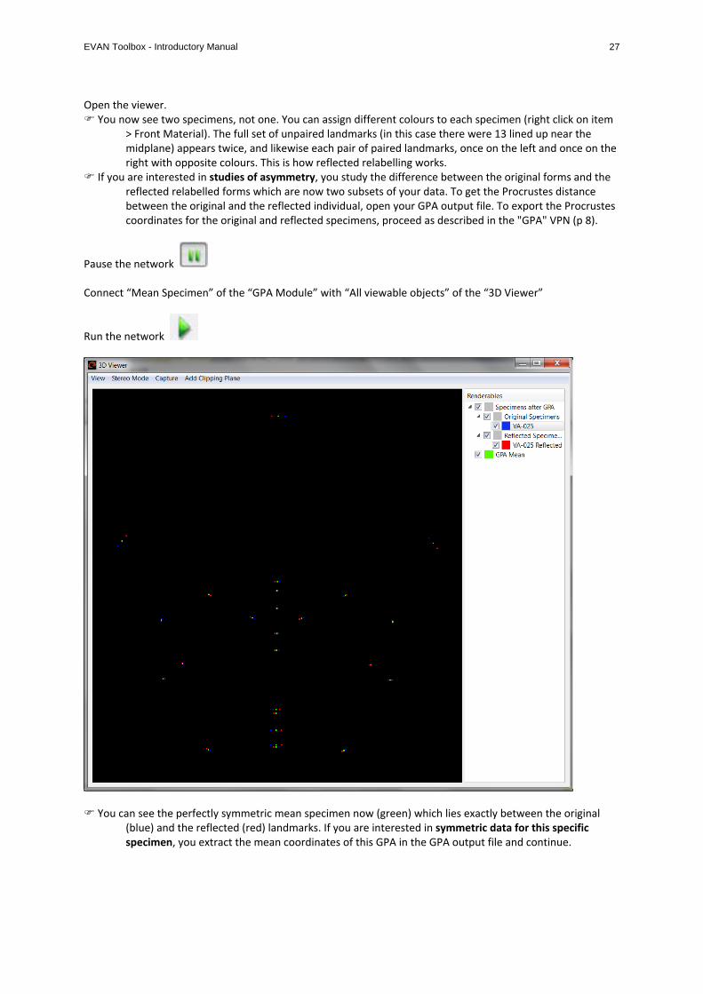
Open the viewer. You now see two specimens, not one. You can assign different colours to each specimen (right click on item

> Front Material). The full set of unpaired landmarks (in this case there were 13 lined up near the midplane) appears twice, and likewise each pair of paired landmarks, once on the left and once on the right with opposite colours. This is how reflected relabelling works.

If you are interested in studies of asymmetry, you study the difference between the original forms and the reflected relabelled forms which are now two subsets of your data. To get the Procrustes distance between the original and the reflected individual, open your GPA output file. To export the Procrustes coordinates for the original and reflected specimens, proceed as described in the "GPA" VPN (p 8).

Pause the network Connect “Mean Specimen” of the “GPA Module” with “All viewable objects” of the “3D Viewer”

Run the network

You can see the perfectly symmetric mean specimen now (green) which lies exactly between the original

(blue) and the reflected (red) landmarks. If you are interested in symmetric data for this specific specimen, you extract the mean coordinates of this GPA in the GPA output file and continue.


8. Reflected relabelling for many specimens

General comment: This network is exactly the same as the previous network; only the data differ (not longer a single specimen, but several). Run the predefined VPN Start ET Open VPN "ReflectedRelabelling" Double‐click node "Import"

Tab "Specimens": Choose the appropriate path and filename for "Datafile" (e.g., " VA_ExerciseDataSet_Humans.txt")

Choose "Pairs.txt" for "Landmark Pairs"

Run the network All specimen are imported this time via the "Import" node. The file defining the paired landmarks is of course needed here too. The "Reflected Relabelling" node works in the same way with many specimens as described above for a

single specimen. The "GPA" node dialogue box comes with all defaults, leave the settings and specify an output file (bottom).

Open the "3D Viewer" and examine the results. Assign a colour (right click on item > Front Material) to the “Original Specimens” and another colour to the

“Reflected Specimens”


Interact with the network For more practice, edit this network.

Pause the network Connect "Mean Specimen" of the "GPA Module" node with "All viewable objects" of the "3D viewer".

Run the network Open the "3D Viewer" Uncheck the "Original Specimens" Uncheck the "Reflected Specimens" You will see an exactly symmetric shape (for instance, looking at it from straight front, all of the unpaired

landmarks lie on a vertical line) of the GPA Mean which is derived from the whole sample. Again, this is exactly what reflected relabelling is supposed to accomplish.

To study asymmetry, see chapter 10 of this manual.


9. Partial Least Squares (PLS) 2‐block shape with shape (face and braincase)

General comment: The VPN itself, the figure above, is actually the best way we know to teach Partial Least Squares. The diagram is far more accessible to the student than any of the usual sets of equations. For instance, the VPN makes it clear how the standard PLS is symmetric between the two data sets (“blocks”) that are being combined. Likewise the flow from left to right corresponds to the way that the student or the user should think of the order in which the analyses are usually reported most effectively. Run the predefined VPN Start ET Open VPN "PLS_2block_shape‐shape" Double‐click upper node "Import"

Tab "Specimens": Choose the appropriate path and filename for "Datafile" (e.g., "VA_ExerciseDataSet_Humans_Face.txt")

Tab "Surface": Choose the appropriate path and filename for "Surface file" (e.g., "VA_ExerciseDataSet_Humans_Face.stl")

Set the number of the specimen to associate this surface with (e.g. #15 for the VA_ExerciseDataSet_Humans.txt) Double‐click lower node "Import"

Tab "Specimens": Choose the appropriate path and filename for "Datafile" (e.g., "VA_ExerciseDataSet_Humans_Braincase.txt")

Tab "Surface": Choose the appropriate path and filename for "Surface file" (e.g., "VA_ExerciseDataSet_Humans_Braincase.stl")

Set the number of the specimen to associate this surface with (e.g. #15 for the VA_ExerciseDataSet_Humans.txt)

Run the network


The following text assumes that you know PLS already. PLS starts with two blocks of variables which in this network are two sets of landmark coordinates that are read in by separate import nodes and turned separately by GPA into two sets of shape coordinates. These two sets of shape coordinates are the inputs for the PLS node. Its outputs drive three separate "Graph Plotters": 1) at the top for the singular warps of the 1st block of shape coordinates, 2) at the bottom for the singular warps of the 2nd block of shape coordinates, and 3) at the far right for the singular warps of one block versus the other.

The first two of these plotters drive one viewer each (working through two "Warpers" that you actually don't have to open) that let you see each singular warp of either block as a surface deformation, grid deformation, etc.

The third graph plotter is the usual statistical display that shows the covariance explained by the PLS. This is what is usually sent for significance testing.

Use the first "Warper" to visualise the effect on the shape of the first block (here, the face in the top row

with slider set to ‐0.1 for the left and +0.1 for the right panel) of an increase in the slider position in the first row (the first “latent variable”). Use the second "Warper" to indicate the effect on the shape of the second block (here, the braincase in the bottom row with same slider setting) of this same change of slider position. These are the two aspects of shape deformation, one for the structure generating the landmarks of the first block and one for the structure generating the landmarks of the second, that have the highest covariance (in Procrustes units) of any such pair.


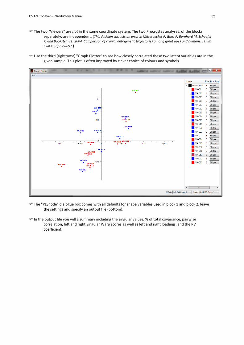
The two "Viewers" are not in the same coordinate system. The two Procrustes analyses, of the blocks separately, are independent. (This decision corrects an error in Mitteroecker P, Gunz P, Bernhard M, Schaefer

K, and Bookstein FL. 2004. Comparison of cranial ontogenetic trajectories among great apes and humans. J Hum

Evol 46(6):679‐697.) Use the third (rightmost) "Graph Plotter" to see how closely correlated these two latent variables are in the

given sample. This plot is often improved by clever choice of colours and symbols.

The "PLSnode" dialogue box comes with all defaults for shape variables used in block 1 and block 2, leave

the settings and specify an output file (bottom). In the output file you will a summary including the singular values, % of total covariance, pairwise

correlation, left and right Singular Warp scores as well as left and right loadings, and the RV coefficient.


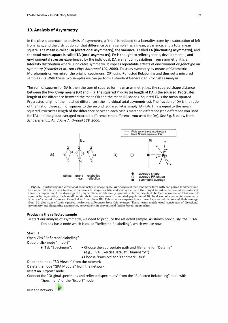
10. Analysis of Asymmetry In the classic approach to analysis of asymmetry, a "trait" is reduced to a laterality score by a subtraction of left from right, and the distribution of that difference over a sample has a mean, a variance, and a total mean square. The mean is called DA (directional asymmetry), the variance is called FA (fluctuating asymmetry), and the total mean square is called TA (total asymmetry). FA is thought to reflect genetic, developmental, and environmental stresses experienced by the individual. DA are random deviations from symmetry, it is a laterality distribution where 0 indicates symmetry. It implies repeatable effects of environment or genotype on symmetry (Schaefer et al., Am J Phys Anthropol 129, 2006). To study symmetry by means of Geometric Morphometrics, we mirror the original specimens (OR) using Reflected Relabelling and thus get a mirrored sample (RR). With these two samples we can perform a standard Generalized Procrustes Analysis. The sum of squares for DA is then the sum of squares for mean asymmetry, i.e., the squared shape distance between the two group means (OR and RR). The squared Procrustes length of DA is the squared Procrustes length of the difference between the mean OR and the mean RR shapes. Squared TA is the mean squared Procrustes length of the matched differences (the individual total asymmetries). The fraction of DA is the ratio of the first of these sum of squares to the second. Squared FA is simply TA ‐ DA. This is equal to the mean squared Procrustes length of the difference between each case's matched difference (the difference you used for TA) and the group averaged matched difference (the difference you used for DA). See Fig. 5 below from Schaefer et al., Am J Phys Anthropol 129, 2006.

Producing the reflected sample To start our analysis of asymmetry, we need to produce the reflected sample. As shown previously, the EVAN

Toolbox has a node which is called "Reflected Relabelling", which we use now. Start ET Open VPN "ReflectedRelabelling" Double‐click node "Import"

Tab "Specimens": Choose the appropriate path and filename for "Datafile" (e.g., " VA_ExerciseDataSet_Humans.txt")

Choose "Pairs.txt" for "Landmark Pairs" Delete the node "3D Viewer" from the network Delete the node "GPA Module" from the network Insert an "Export" node Connect the "Original specimens and reflected specimens" from the "Reflected Relabelling" node with

"Specimens" of the "Export" node.

Run the network


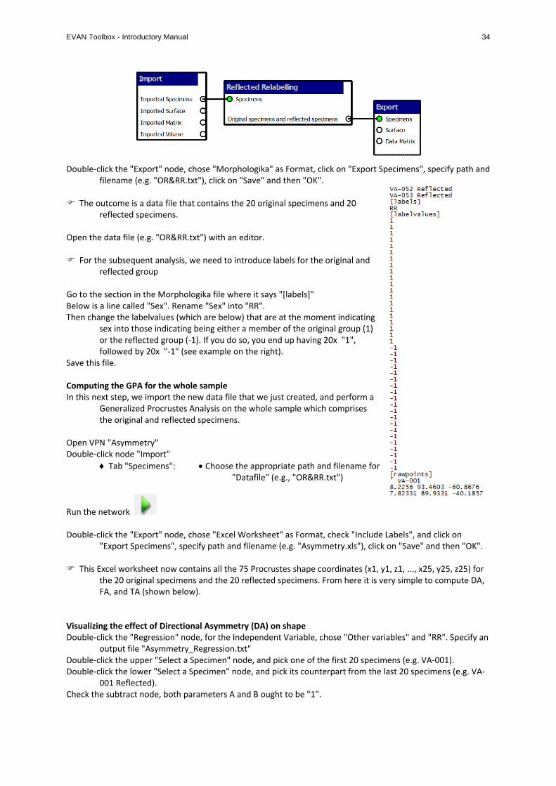
Double‐click the "Export" node, chose "Morphologika" as Format, click on "Export Specimens", specify path and filename (e.g. "OR&RR.txt"), click on "Save" and then "OK".

The outcome is a data file that contains the 20 original specimens and 20

reflected specimens. Open the data file (e.g. "OR&RR.txt") with an editor. For the subsequent analysis, we need to introduce labels for the original and

reflected group Go to the section in the Morphologika file where it says "[labels]" Below is a line called "Sex". Rename "Sex" into "RR". Then change the labelvalues (which are below) that are at the moment indicating

sex into those indicating being either a member of the original group (1) or the reflected group (‐1). If you do so, you end up having 20x "1", followed by 20x "‐1" (see example on the right).

Save this file. Computing the GPA for the whole sample In this next step, we import the new data file that we just created, and perform a

Generalized Procrustes Analysis on the whole sample which comprises the original and reflected specimens.

Open VPN "Asymmetry" Double‐click node "Import"

Tab "Specimens": Choose the appropriate path and filename for "Datafile" (e.g., "OR&RR.txt")

Run the network Double‐click the "Export" node, chose "Excel Worksheet" as Format, check "Include Labels", and click on

"Export Specimens", specify path and filename (e.g. "Asymmetry.xls"), click on "Save" and then "OK". This Excel worksheet now contains all the 75 Procrustes shape coordinates (x1, y1, z1, ..., x25, y25, z25) for

the 20 original specimens and the 20 reflected specimens. From here it is very simple to compute DA, FA, and TA (shown below).

Visualizing the effect of Directional Asymmetry (DA) on shape Double‐click the "Regression" node, for the Independent Variable, chose "Other variables" and "RR". Specify an

output file "Asymmetry_Regression.txt" Double‐click the upper "Select a Specimen" node, and pick one of the first 20 specimens (e.g. VA‐001). Double‐click the lower "Select a Specimen" node, and pick its counterpart from the last 20 specimens (e.g. VA‐

001 Reflected). Check the subtract node, both parameters A and B ought to be "1".


What the network does is to take the "Predicted Values" which are the means for both groups, and then

subtract the reflected specimens from the original specimens to get a warp vector. We just need to chose any specimen from the original specimens for the upper "Select a Specimen" node, and any other from the reflected specimens for the lower. The "3D Viewer" then displays the average configuration for original and reflected specimens, and allows you to warp the shape along the trajectory of directional asymmetry (DA). Beside this visualization, you also get the percentage of explained variance from the output of the regression, but this is not a useful quantity.

Open the "Warper" and the "3D Viewer". You find three sets of coordinates in the graph. Change the colour of

the average of the original specimens to blue (they come on top as "Selection>Ungrouped>VA‐001"), the average of the reflected specimens to red (they come second as "Selection>Ungrouped>VA001 Reflected"), and the "Warped Landmarks" to yellow.


Drag the slider of the "Warper" to visualize the directional asymmetry (DA). If the slider is on "0", the configuration is exactly at the stage of the average original specimens, if it is on "1", it is exactly on the average reflected specimens. Moving the slider outside this range is exaggerating the effects of DA.

You may get the regression coefficients using the "Export" node.

Pause the network Connect "Regression Coefficients" from the "Regression" node with "Data Matrix" from the "Export"

node

Run the network Double‐click the "Export" node, chose the tab "Matrix", Format "Excel Worksheet", check "Include

Labels", and click on "Export Matrix", specify path and filename (e.g. "Asymmetry_RegrCoeff.xls"), click on "Save" and then "OK".

You can of course add a surface as well for better visualization of the asymmetry.

Pause the network Specify a surface file in the "Import" node Connect "Imported Surface" of the "Import" node with "Surface" of the "GPA Module" node. Connect "Mean Surface" of the "GPA Module" node "Base Surface" of the "Warper", and "Warped

Surface" of the "Warper" with "All viewable objects" of the "3D Viewer".

Run the network Drag the slider to see the effect on the surface.

We cannot visualize FA in a similar way because our EVAN Toolbox cannot perform analyses that involve case‐by‐case matching !

DA exaggerated in the direction of originals DA exaggerated in the direction of reflected


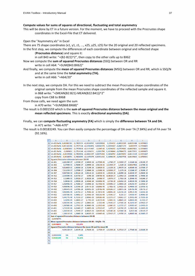
Compute values for sums of squares of directional, fluctuating and total asymmetry This will be done by ET in a future version. For the moment, we have to proceed with the Procrustes shape

coordinates in the Excel‐File that ET delivered. Open the "Asymmetry.xls" in Excel There are 75 shape coordinates (x1, y1, z1, ..., x25, y25, z25) for the 20 original and 20 reflected specimens. In the first step, we compute the differences of each coordinate between original and reflected shape

(Procrustes distance) and square it: in cell B43 write: "=(B2‐B22)^2", then copy to the other cells up to BX62 Now we compute the sum of squared Procrustes distances (SSQ) between OR and RR

write in cell A64: "=SUM(B43:BX62)" And finally, we compute the mean of squared Procrustes distances (MSQ) between OR and RR, which is SSQ/N

and at the same time the total asymmetry (TA). write in cell A66: "=A64/20" In the next step, we compute DA. For this we need to subtract the mean Procrustes shape coordinates of the

original sample from the mean Procrustes shape coordinates of the reflected sample and square it. in B68 write: "=(MEAN(B2:B21)‐MEAN(B22:B41))^2" copy from C68 to BX68 From those cells, we need again the sum in A70 write: "=SUM(B68:BX68)" The result is 0.0001559 which is the sum of squared Procrustes distance between the mean original and the

mean reflected specimens. This is exactly directional asymmetry (DA). Finally, we can compute fluctuating asymmetry (FA) which is simply the difference between TA and DA. in A71 write: "=A66‐A70" The result is 0.00183249. You can then easily compute the percentage of DA over TA (7.84%) and of FA over TA

(92.16%).

EVAN-Toolbox IntroductoryManual...

Documents

Transcript of EVAN-Toolbox IntroductoryManual...