EVALUATION OF USING SWARM INTELLIGENCE TO PRODUCE FACILITY...

EVALUATION OF USING SWARM INTELLIGENCE TO PRODUCE FACILITY LAYOUT SOLUTIONS

By

Andrew Bao Thai B.S., University of Louisville, 2006

A Thesis Submitted to the Faculty of the

University of Louisville J. B. Speed School of Engineering

in Partial Fulfillment of the Requirements for the Professional Degree

MASTER OF ENGINEERING

Department of Computer Engineering and Computer Science

May 2007

i

EVALUATION OF USING SWARM INTELLIGENCE TO PRODUCE FACILITY LAYOUT SOLUTIONS

Submitted By

__________________________________ Andrew Bao Thai

A Thesis Approved on

___________________________________ (Date)

by the Following Reading and Examination Committee:

__________________________________ Eric Rouchka, Thesis Director

Computer Engineering and Computer Science

__________________________________ Tim Hardin


__________________________________ Gail DePuy

Industrial Engineering

ii

DEDICATION

This thesis is dedicated to my parents,

Mr. Danh Kim Thai

and

Mrs. Thanh Le Thai.

Thank you for everything.

iii

ACKNOWLEDGEMENTS

First, I would like to thank my thesis director, Dr. Eric C. Rouchka, for his

direction and guidance. I would also like to thank members of my thesis committee, Tim

Hardin and Gail DePuy, for driving the project and providing advice on how to get the

job done. Finally, I would like to thank the members of the Bioinformatics Research

Group, especially Elizabeth Cha, for making the Bioinformatics lab an environment

conducive to the project’s progress.

iv

ABSTRACT

The facility layout problem is a combinatorial optimization problem that involves

determining the location and shape of various departments within a facility based on

inter-department volume and distance measures. An optimal solution to the problem will

yield the most efficient layout based on the measures.

The application of Particle Swarm Optimization (PSO) was recently proposed as

an approach to solving the facility layout problem. With PSO, potential solutions are

produced by dividing departments into swarms of Self-Organizing Tiles (SOT). By

following a set of simple behavioral rules based on social information gathered from the

environment, the tiles cooperate to produce solutions in a very short amount of time.

Initial results provided improvements over CRAFT, one of the primary methods currently

used for facility layout.

The main contribution of this thesis work entails evaluating the use of swarm

intelligence to produce optimal facility layouts as well as the use of shape measures to

assess the quality of produced layouts. The major achievement of this thesis is the design

and implementation of a tool that could produce facility layout solutions using Self-

Organizing Tiles (SOT). This thesis advances the swarm paradigm by introducing

alternative pathways for achieving contiguity of departments.

This thesis utilizes the tool to examine the convergence of SOT on an enumerated

optimum for a layout dataset, which requires the exhaustive evaluation of all

v

permutations of a grid layout. The tool was also used to examine the effect of granularity

on the ability of SOT to converge on facility layout solutions. A shape metric was utilized

as a means of evaluating the quality of produced solutions based on the regularity of the

shape of departments, and found that SOT produces fairly regular layouts when

granularized to nine tiles per department. Finally, SOT was compared with other

algorithms the experimental results revealed that SOT provided minor improvements

over currently used methods.

vi

TABLE OF CONTENTS

LIST OF TABLES............................................................................................................ vii

LIST OF FIGURES ......................................................................................................... viii

I. BACKGROUND......................................................................................................... 1

A. The Facility Layout Problem ................................................................................. 1

B. Material Handling Costs......................................................................................... 4

C. Block Layout Representation ................................................................................. 7

D. Existing Models and Approaches .......................................................................... 8

E. Shape Measures .................................................................................................... 11

F. Particle Swarm Optimization (PSO)..................................................................... 12

G. Motivation............................................................................................................ 13

II. USING SWARM INTELLIGENCE........................................................................ 15

A. Model Description................................................................................................ 15

B. Experimental Design ............................................................................................ 18

III. IMPLEMENTATION............................................................................................. 21

A. Reading an Input File........................................................................................... 21

B. Data Structures ..................................................................................................... 21

C. Complete Enumeration of a Problem................................................................... 22

D. User Interface....................................................................................................... 23

E. Self-Organizing Tiles (SOT) ................................................................................ 24

IV. RESULTS............................................................................................................... 29

A. Phase I .................................................................................................................. 31

B. Phase II................................................................................................................. 35

C. Phase III................................................................................................................ 41

D. Phase IV ............................................................................................................... 41

V. DISCUSSION .......................................................................................................... 43

VI. CONCLUSION....................................................................................................... 45

REFERENCES ................................................................................................................. 47

APPENDIX I: LIST OF ABBREVIATIONS................................................................... 50

CURRICULUM VITAE................................................................................................... 51

vii

LIST OF TABLES

TABLE I. Volume matrix for data set T12....................................................................... 30

TABLE II. Volume matrix for data set T14 ..................................................................... 31

TABLE III. Results for data set T12, 1 tile per department ............................................. 32

TABLE IV. Results for data set T14, 1 tile per department ............................................. 34

TABLE V. Results for data set T12, 4 tiles per department ............................................. 35

TABLE VI. Results for data set T14, 4 tiles per department............................................ 37

TABLE VII. Results for data set T12, 9 tiles per department .......................................... 38

TABLE VIII. Results for data set T14, 9 tiles per department ......................................... 39

TABLE IX. Pearson correlation coefficient for best known score................................... 40

TABLE X.Comparison of Results of SOT with Layout Swarm and CRAFT.................. 41

TABLE XI. Calculated Shape Measures for Layouts with Best Scores........................... 42

viii

LIST OF FIGURES

FIGURE 1. A few possible layout types............................................................................. 6

FIGURE 2. Example of a block layout............................................................................... 7

FIGURE 3. Shape measure captures deterioration of department shape.......................... 12

FIGURE 4. Initial grid of 12 departments; randomized tile locations.............................. 17

FIGURE 5. Equivalent layouts with various levels of granularity ................................... 19

FIGURE 6. Sample screenshot of user interface .............................................................. 23

FIGURE 7. Example initial grid layout with fixed departments ...................................... 24

FIGURE 8. VDP Histogram for SOT (1-tile) and enumeration on T12 data set.............. 33

FIGURE 9. VDP Histogram for SOT (1-tile) and enumeration on T14 data set.............. 34

FIGURE 10. VDP Histogram for SOT (4 tiles per department) on T12 data set ............. 36




1

I. BACKGROUND

The facility layout problem [1] is a combinatorial optimization problem that

involves determining the location and shape of various departments within a facility

based on inter-department volume and distance measures. An optimal solution to the

problem will yield the most efficient layout based on the measures. The application of

Particle Swarm Optimization (PSO) was recently proposed as an approach to solving the

facility layout problem [2]. Swarm intelligence offers a robust and adaptable approach

that can produce good solutions of good quality in a relatively short amount of time for

complex problems. The objective of this thesis work entails evaluating the use of swarm

intelligence to produce solutions for the facility layout problem as well as the

incorporation of shape measures to calculate the quality of layouts.

A. The Facility Layout Problem

Facilities planning is an essential function to ensure the successful establishment

of a production operation. It may entail either adaptation of an existing facility to support

dynamic materials handling requirements or design of a new facility in conjunction with

advanced product manufacturing processes to realize overall profitability. In a broad

sense, facilities planning is one of the most important steps in planning and constructing a

new facility or in expanding an existing facility, and it involves a considerable amount of

2

investment money. Facility layout should be performed prior to installing materials

handling and manufacturing process equipment and should be carefully prepared to avoid

pitfalls after implementation. Poorly planned facilities with improper equipment result in

huge initial investments and become a constant drain on the profitability of an

organization. It may also result in premature obsolescence of the facility.

Facility layout should be a thoughtful, well-planned process to integrate

equipment, materials, and manpower for processing a product in the most efficient

manner. Materials should, for example, move from receiving through production to

shipping in the shortest time possible and with the least amount of handling. This is

important because the more time material is in the plant the more it costs in terms of

inventory, obsolescence, overhead, and labor.

The facility layout problem [1] is a well-studied combinatorial optimization

problem that arises in a variety of production facilities. It is concerned with determining

the most efficient physical arrangement of indivisible departments with unequal area

requirements within a facility. The problem consists of assigning each department to a

specific location in the facility, while considering the variability of interaction

relationships between departments. As defined by Bozer et al. [3] the objective of the

facility layout problem is to minimize the material handling costs inside a facility subject

to two sets of constraints: (1) department and floor area requirements and (2) department

locational restrictions. The second of these might include requirements that departments

cannot overlap, must be placed within a facility, and some must be fixed to a location or

cannot be placed in specific regions. A layout’s efficiency is typically measured in terms

of material handling costs.

3

Direct components of material handling cost include depreciation of material

handling equipment, variable operating costs of equipment, and labor expenses for

material handlers [4]. The minimization of material handling cost, a distance-based

objective, reduces material movement. According to Askin and Standridge [4], “reduced

material movement translates into reductions in aisle space, lower work-in-process (WIP)

levels and throughput times, less product damage and obsolescence, reduced storage

space and utility requirements, simplified material control and scheduling, and less

overall congestion”. Hence, when minimizing material handling cost, the other objectives

are achieved simultaneously.

The effect of facility layout on WIP can be seen by considering the following

examples. If successive processes are immediately adjacent, a single unit is moved at a

time, as in an assembly line. If the next process is across the aisle, the handling lot size is

a unit load. If the next process is across the building, the handling lot size may be at least

an hour’s supply of product because more frequent collection and transport is impractical.

If the next process is in another building, the handling lot size could be at least one day’s

production. Potential orders-of-magnitude differences in WIP levels can be observed

based on the layout.

McKendall, Noble, and Klein [5] citing Mecklenburgh [6] and Francis et al. [7]

provide a list of objectives that are generally considered in determining an efficient

layout, including:

• Minimize material handling time and frequency of handling.

• Minimize capital and operating cost in equipment and plant.

• Increase effective and economical use of space.

4

• Facilitate the manufacturing process and flow of operation.

• Maintain flexibility of arrangement and operation.

• Provide for safe and efficient construction.

B. Material Handling Costs

Material handling costs are approximated with one or more of the following

parameters: interdepartmental flows, ijv (the flow volume measured in trips per unit time

from department i to department j); unit-cost values, ijc (the cost to move one unit load

one distance unit from department i to department j, including cost of material handling

equipment, labor cost, and inventory cost for time in transit); and the department

closeness ratings, ijr (the numerical value of a closeness rating between departments i

and j). Alternatively, these parameters can be used as subjective weights including safety,

customer importance, and other factors as well as standard accounting costs. If all

movement is of equal concern, all ijc may be set to 1. These parameters are used in two

common surrogate material handling cost functions [7].

The first of the two surrogate material handling functions is based on

departmental adjacencies:

max ))(( iji j

ij xr∑∑ (1)

where ijx equals 1 if departments i and j are adjacent, and 0 otherwise. Such an objective

is based on the material handling principle that material handling costs are reduced

significantly when two departments are adjacent.

5

The second of the two surrogate material handling cost functions is based on

interdepartmental distances:

min ))()(( ijiji j

ij dcv∑∑ (2)

where ijd is the distance from department i to department j. This objective is based on the

material handling principle that material handling costs increase with the distance the unit

load must travel. The distance is primarily measured in one of two ways.

The most accurate distance measure is the distance between input/output (I/O)

points. This distance is measured between the specified I/O points of two departments

and in some cases is measured along the aisles when traveling between two departments.

The major drawback of this accurate measure is that one does not know the location of

the I/O points (or aisles) until one has developed a detailed layout.

The input and output points of the departments are typically unknown.

Consequently, the department centroid is widely used to approximate the department I/O

point. One of the shortcomings of centroid-to-centroid (CTC) distances is that the optimal

layout is one with concentric rectangles [8]. An algorithm based on CTC attempts to

align the centroid as close as possible, which may make the departments very long and

narrow [9]; and a department that is L-shaped may have a centroid that falls outside of

the department [7] (see Figure 1).

6

FIGURE 1. A few possible layout types--concentric rectangles (a), linear columns (b), L-shaped (c)

For each of the aforementioned distance measures, there are two metrics used to

measure the distance between two points. Rectilinear distance is most commonly used

metric because it is based on travel along paths parallel to a set of perpendicular

(orthogonal) axes [10]. The second metric, Euclidean distance, is appropriate when

distances are measured along a straight-line path connecting two points [10]. If there is a

large amount of volume flow between two departments, then the departments should

logically be assigned locations so that they are near each other to minimize transportation

and handling costs.

The objective is to minimize the sum of the product of all the flow values, unit

cost and rectilinear distance between department centroids. The unit cost (i.e. the cost of

moving a unit load 1 distance unit between departments) is assumed to be equal to one, as

the flow values can be defined as the product of the flow between departments and their

unit cost. Thus, the primary objective can be achieved by minimizing the sum of all

products of flow values and rectilinear distance between department centroids.

7

C. Block Layout Representation A typical approach to the facility layout problem is to combine tasks or equipment

into functional groups, or blocks. Once knowledge of the materials flow, process details,

and support activities is known, it is possible to locate different blocks on the layout

based on their relationships with each other. Specifying the relative location and size of

each department within a facility, this common representation of solutions to the facility

layout problem is referred to as the block layout [11]. Block layouts are used to provide

preliminary information to architects and engineers involved in the construction of a new

facility. The block layout is typically represented in either a discrete or continuous

fashion. A discrete representation of the block layout uses a collection of grids to

represent departments. However, a continuous representation uses the centroid, area,

perimeter, width and/or length of a department to specify the exact location of the

department within a facility layout. In the literature, most of the facility layout algorithms

use a discrete representation to generate the block layout [5].

FIGURE 2. Example of a block layout

8

Once a diagram of the block layout has been prepared (see Figure 2), a

manufacturing engineer then can perform further work to make the detailed layout, which

specifies exact department locations, aisle structures, input/output (I/O) point locations,

and the layout within each department.

In this thesis, we are not concerned with specific details such as the position and

angular orientation of a worker’s bench or where the power outlets should be located.

Instead, we concentrate on the relative location of the set of major physical resources

with respect to each other. A resource may be a single, large machine for a small problem,

but it would more likely be a process department, group, or assembly line for full

problems. These resources are hereafter referred to as departments, defined to be spaces

in a facility used for providing services, administrative processes and production. The

goal is to produce a block layout showing the relative positioning of departments.

D. Existing Models and Approaches

A number of models have been developed for the discrete representation of the

facility layout problem. The facility layout problem was first modeled as a Quadratic

Assignment Problem (QAP) by Koopmans and Beckmann [12], where all the

departments have equal sizes and all locations are fixed a priori. The QAP formulation

assigns each department to exactly one location and exactly one department to each

location. The cost of assigning a department a particular location is dependent on the

location of interacting departments. This dependency leads to the quadratic objective that

inspires the problem's name.

9

If actual departments are represented in the model by a set of pseudo-

subdepartments relative in number to the total area of each department, this expanded

model resembles a block layout. Solutions for the QAP are based on variations of the

branch-and-bound approaches initially proposed by Gilmore [13] and Lawler [14] . Sahni

and Gonzalez [15] showed that the QAP is NP-complete, which implies that to guarantee

an absolute optimal solution would require the evaluation of all possible solutions.

According to Meller and Gau [10], optimal solutions to general cases of the QAP can

only be found for problems with less than 18 departments. In addition, due to the

constrained multi-objective nature of real facility layout problems, truly “optimal”

layouts that satisfy all objectives and constraints are not practically achievable.

According to Liao [16], Kusiak and Heragu [1], and others, the unequal-area

facility layout problem may be modeled as a modified QAP by dividing the departments

into small grids with equal area, assigning a large artificial flow between those grids of

the same department to ensure that they are not split, and solving the resulting QAP.

However, due to the increase in "departments" with this approach, it is not possible to

solve even small problems with a few unequal-area departments [10]. In addition, Bozer

and Meller [17] show that such an approach is ineffective because it implicitly adds a

department shape constraint.

A few models have been developed for continuous representations of the facility

layout problem. Montreuil [17] presented a Mixed-Integer Programming (MIP) model for

the facility layout problem based on a continuous representation. A similar model was

developed by Heragu and Kusiak, formulated as a linear continuous program with

absolute values in the objective function and constraints and a linear mixed integer

10

program [18]. In their formulation the location of sites need not be known a priori and

the areas of the departments are unequal, but the department dimensions were fixed.

The MIP formulation is more difficult to solve computationally. Consequently,

optimal solutions (from using the MIP formulation) to problems with nine or more

departments have not been reported in the literature. However, the MIP model does have

advantages over QAP-based models. With the MIP model, departments may have various

shapes and sizes. In addition, the shape of the departments is controlled, and irregular-

shaped departments are not an issue [5]. In the literature, irregular-shaped departments

are considered to be departments which may be very long, narrow, or non-rectangular.

Departments are initially rectangular in shape during the layout planning phase,

and it is desirable that they remain being rectangular after an algorithm is applied. QAP-

based models and some graph theoretic models generate irregular-shaped departments by

allowing departments to assume regular and/or irregular shapes. Algorithms which result

in irregular-shaped departments include: CRAFT [19]; CORELAP [20]; SPIRAL [21];

and MULTIPLE [3].

Algorithms have been developed to solve the facility layout problem may be

classified as either optimal algorithms or suboptimal algorithms. Optimal algorithms such

as branch-and-bound algorithms [22] and cutting plane algorithms [23] have a high

computational time and memory complexity [1]. As a result, researchers have developed

suboptimal algorithms for solving the facility layout problem that require low

computational time but produce good solutions of good quality. These solutions may be

close to the optimum, but even when the best solution is obtained it is hard to prove its

optimality. Thus, one might ask if it is worthwhile to use algorithms which produce

11

solutions of better quality at the expense of computational time rather than algorithms

which produce solutions of relatively lower quality at very low computational times.

Ideally, algorithms which solve the facility layout problem must be able to

produce good quality solutions, have relatively low computational requirement, be able to

solve problems with facilities of equal and unequal areas, and provide the user flexibility

with respect to facility configuration (i.e. fixing locations).

E. Shape Measures

In order to control department shape, Liggett and Mitchell [24] as well as Bozer et

al. [3] presented “shape measures” that are used to detect and penalize irregularly shaped

departments. This raises a concern that using shape measures may result in generating

substandard layouts such that optimal and feasible solutions may be omitted [8].

While the human eye is capable of making judgments concerning shape, a

computer program requires a formal measure which must also be easy to compute.

Freeman [25] noted that the perimeter of an object with a fixed area increases as it

becomes more irregular in shape. Letting iP denote the perimeter of department i, i

i

AP can

be used to measure shape irregularity. A non-circular object would have a minimized

perimeter if the object is square shaped. Therefore, the minimum perimeter for

department i, *iP , is equal to iA4 . Assuming that a square represents the ideal

department shape, the normalized shape measure for department i, iΩ , is given by:

12

iΩ =ii

ii

APAP

//

* = *i

i

PP =

i

i

AP

4=

41

iP 5.0−iA . (3)

With the above measure, as a department’s shape becomes more irregular, its iΩ value

increases. According to Bozer et al. [3], reasonable shapes for a department are generally

obtained if an upper limit on iΩ is kept under 1.50. This measure is also more effective

than the two alternative shape measures that were proposed by Liggett and Mitchell [24].

The first one divides the area of the smallest enclosing rectangle by the area of the

department itself. The second measure divides the length of the smallest enclosing

rectangle by its width. As seen in Figure 3, the iΩ value captures the deterioration of

department shape.

FIGURE 3. Shape measure captures deterioration of department shape.

F. Particle Swarm Optimization (PSO)

Recently, Hardin and Usher [2] proposed the application of Particle Swarm

Optimization (PSO), a population based optimization technique developed by Kennedy

and Eberhart [26], as an approach to solving the facility layout problem. The system is

initialized with a population of random solutions and searches for optima by updating

potential solutions over generations. Unlike genetic algorithms, PSO has no evolution

13

operators such as crossover and mutations. With PSO, potential solutions to the facility

layout problem are produced by dividing departments into groups of Self-Organizing

Tiles (SOT). By following a set of simple behavioral rules based on social information

gathered from the environment, the tiles “fly” through the problem space and evolve one

solution to a new and potentially more efficient solution. Through this emergent behavior,

the tiles cooperate and converge upon solutions with contiguous departments in a very

short period of time. Its primary drawback is that it produces solutions with

nonrectangular departments. Robust and adaptable to a variety of intractable facility

configurations, Hardin and Usher’s Layout Swarm has provided improved results

compared to CRAFT, one of the primary methods currently used for facility layout.

G. Motivation

The improved results suggested that the application of swarm intelligence for

facility layout is a promising area of further research. In addition, enhancements in

implementation could potentially yield further improvements in performance. The

objective of this thesis is to evaluate this approach and to incorporate shape measures to

penalize the calculated efficiency of layouts with irregularly-shaped departments. The

supplementary use of shape measures could be a way to improve this approach by

ensuring that the algorithm yields optimal layouts of good quality.

This approach will be evaluated in four phases. In the first phase of evaluation, all

departments are of equal size and each department is represented by a single tile. This

phase will examine how well SOT approach optimal solutions for various facility layouts

where it is computationally practical to evaluate all possible arrangements of departments.

14

The second phase of evaluation will add a layer of granularity to the first phase. In

this phase, each department is represented by a group of tiles. All departments are of

equal size. Therefore, the departments will have the same number of tiles. This phase will

examine the effect of granularity on the performance of SOT.

The third phase of evaluation will compare the performance of SOT against the

results of other algorithms, including Hardin and Usher’s Layout Swarm implementation.

The fourth and final phase will incorporate shape measures to the second phase.

The shape measures will be used in alternatively calculating the efficiency of a layout to

consider its quality based on the regularity of department shapes. This phase will examine

the effect of granularity on the quality of solutions produced by SOT.

15

II. USING SWARM INTELLIGENCE

Particle Swarm Optimization exhibits some evolutionary attributes in that a series

of particles, each representing a solution, are allowed to fly through a solution space. The

particles cooperate to converge upon a solution. Each department is represented by a

number of tiles that corresponds to the department’s relative size in the overall facility.

Each tile is given a simple rule by which to interact with the other tiles so that the tiles

ultimately self-organize to produce a practical and contiguous solution. From this

contiguous solution, each tile uses another simple rule to evolve one solution toward a

new and potentially more efficient solution.

A. Model Description The facility that will be analyzed is divided into a rectangular grid of fixed

dimensions that correspond with the length and width of the facility. Each element in the

grid, represented by a tile, is a member of the swarm. Each department in the facility is

represented by a group of tiles. The number of tiles in a group is proportionally based on

the department’s relative area with respect to the entire facility. Parameters can be

configured if a department is required to be in a fixed position.

To compare solutions of various algorithms, material handling costs were

measured with the Volume-Distance Product (VDP) metric—a common measure of

16

facility layout efficiency. The layout with the lowest VDP is considered to be the most

efficient. The VDP is defined as:

))()(( ijiji j

ij dcv∑∑ (4)

where ijv is the interdepartmental flow volume from department i to department j, ijc is

the transportation cost from department i to department j, and ijd is the distance from

department i to department j.

Interdepartmental flow volume is measured in trips per unit time from department

i to department j. All interdepartmental flow volumes are quantified by a volume matrix.

Interdepartmental transportation cost is measured by the overall cost required to

move one unit load one distance unit from department i to department j, including the

cost of material handling equipment, labor, and inventory for time in transit. All

interdepartmental cost values are quantified by a cost matrix.

The distances between departments are measured as the distance between

input/output (I/O) points. Since the I/O points of the departments are unknown, the

department centroid is used to approximate the I/O point. For a metric to measure the

distance between centroids rectilinear distance was chosen because it is based on travel

along paths parallel to a set of perpendicular axes inherently alluded to by the facility’s

rectangular grid representation.

The interaction and movement of tiles is determined by two rules. First, a tile will

move toward the centroid of a department which it has a flow volume relationship with.

Second, a tile will move towards the centroid of its own department. The first rule is

17

applied to generally move tiles closer to departments with which they have volume

relationships. The second rule is applied so that all tiles of a department move until they

are contiguous and the department is not split.

To initialize the algorithm, tiles (without a fixed location requirement) are

randomly assigned locations in the layout grid (see Figure 4).

FIGURE 4. Initial grid of 12 departments with 4 tiles per department; randomized tile locations.

For each iteration, the algorithm primarily focuses on the volume flow between

two departments. First, a department is selected at random. This department, dfrom, is

designated to be the source of volume flow between itself and another department. A

second department is selected using the “roulette wheel” method [27] with more weight

given to departments that have higher volume relationships with the source department.

This department, dtarget, is considered to be the destination of interdepartmental flow. All

tiles that belong to department dfrom are allowed to move towards the centroid of

department dtarget. The tiles that are nearest to the centroid of dtarget are allowed to move

first. A tile moves around by swapping locations with the neighboring tile that is

currently in the direction it needs to go for it to be closer to its target location.

18

After all tiles have moved, every tile in the layout grid is allowed to move towards

the centroid of its own department until contiguity is achieved for every department.

Once overall contiguity is achieved, the current layout is accepted as a new solution. The

solution is scored using the VDP metric. If this solution has a score that is better than the

best known score, its layout is also recorded. This process is repeated for a predetermined

number of iterations.

B. Experimental Design To evaluate the use of Self-Organizing Tiles (SOT) for facility layout, the

performance of the algorithm in approaching the optimum scores for two data sets was

examined. In the first phase, non-fixed departments were represented by a single tile.

With each department represented by a single tile, the layout of twelve departments can

be reduced to a permutation. The optimum score for each dataset was obtained by

examining all possible permutations. Both datasets have been designed with 12 non-fixed

departments because it is feasible to fully enumerate all possible layouts within a

reasonable amount of time. The exhaustive enumeration of the domain is impractically

large for more than 12 single-tile departments. Scoring all 12!, or 4.79 × 108, layouts for

each dataset requires 49 CPU hours to process on a 2.13 GHz AMD Athlon MP desktop

computer.

Once the optimum score was obtained, the algorithm with single-tile departments

was allowed to run for 60,000 iterations for each of 30 trials. During each trial, the score

was recorded for each iteration. If a solution has a score that is better than the previously

best known score, its layout is recorded.

19

For the second phase, granularity was added to the datasets by dividing each

department into four tiles to obtain initial layouts that are equivalent to the single-tile

representation (see Figure 5). The algorithm was allowed to run for 20,000 iterations for

each of 30 trials. This representation allowed us to examine the effect of granularity on

the scored performance of SOT. Additional granularity is examined by representing each

department by nine tiles. Representation by multiple tiles allows a department to become

more flexible in movement and orientation, but leads to possible quality degradation as

departments tend to become irregular-shaped.

FIGURE 5. Equivalent layouts with various levels of granularity

During the third phase, the performance of SOT was compared to Hardin and

Usher’s Layout Swarm and CRAFT.

After all experiments have been performed, Bozer’s [3] shape measure was used

in the fourth and final phase to assess the quality of the solutions produced by SOT.

Square or rectangular departments are desirable and yield higher quality because they are

compact whereas irregular-shaped departments are not. An optimal solution consisting of

a series of concentric rectangles with centroids in the same position would yield a VDP

20

score of zero, but such a layout is not a practically feasible solution and would be poorly

rated by the shape measure.

21

III. IMPLEMENTATION

The SOT tool was developed in the C# programming language. The IDE

(Integrated Development Environment) used for code development was Microsoft®

Visual Studio® 2005.

A. Reading an Input File

The program reads a formatted input file that contains the input parameters for the

facility. The first line of the file contains n, the number of departments. The second line

of the file contains r and c—the number of rows and columns, respectively. The third line

marks the beginning of the data section that describes the number of tiles for each

department. This section also describes a department’s exact location if it is fixed. The

following section describes the volume matrix. The last section describes the cost matrix.

B. Data Structures

The values for n, r, and c are stored in integer variables named numDepts,

numRows, and numCols, respectively. From this information, a matrix of integer values

named deptLayout is initialized of size r x c to represent the layout. The values in this

matrix indicate to which department each tile element belongs. A similar matrix named

bestLayout will store the layout of the solution with the best known score. The current

and best known scores are stored in variables of type double named currScoreVDP and

22

bestScoreVDP. Tiles are represented as objects that know their location in the layout as

well as the department to which they are assigned. Departments are represented as objects

that contain a list of its tiles, a boolean to indicate whether or not the department is fixed,

and its size. From the list of tiles, a department is able to calculate its centroid.

C. Complete Enumeration of a Problem

A recursive iterator was used to evaluate all permutations of an array of

departments. Given an integer array v[] of elements, an integer n (the number of

elements), and an integer i (the index), the recursive function generates the permutations

of the array from element i to element n-1. The pseudocode for the recursive iterator is as

follows:

void enumerate (int[] v, int n, int i)

{ if (i == n)

{ Assign each department a location based on its

current order in the array.

Score the current layout.

else

{ for (j = 1; j < n; j++)

Swap elements i and j.

enumerate (v, n, i+1)

Swap back elements i and j.

}

}

23

D. User Interface The user interface (Figure 6) provides a visual representation of the program’s

processes and capabilities with an intuitive layout that is easy to understand without

revealing the complex implementation required to complete tasks. Once a dataset is

loaded from a file using the Load button, the program will generate a default layout

where tiles are assigned departments in sequential order. Tiles for a department with a

fixed location requirement are assigned in the layout first. After all tiles have been

assigned departments, the program will display a graphical representation of the grid

layout (Figure 7).

FIGURE 6. Sample screenshot of user interface

Once all tiles of the layout have been assigned departments, the interface allows

the user to modify or analyze the layout. If the user wishes to swap tiles, the user simply

has to mouse-click on the two tiles. The user may randomize the tile locations in the

layout using the Shuffle button. The user is able to score the layout using the VDP metric

24

FIGURE 7. Example initial grid layout with fixed departments (1 and 2) at any time by clicking on the Score button. Each time the layout is scored, the program

updates a text display to reflect the current and best known scores. In addition, the

program will update curves on a graph plot to reflect the current and best known scores.

The graph plot was implemented using an open-source charting class library written in

C# named ZedGraph [http://zedgraph.org/].

E. Self-Organizing Tiles (SOT)

Once the layout has been generated from the input file, the SOT algorithm is

allowed to run. First, a source department is selected at random. Then, a target

department is selected using the “roulette wheel” method. Using the volume matrix, the

target department is selected probabilistically based on the relative distribution of volume

from the source department. The centroid of the target department is then calculated so

that the tiles of the source department can swap in the direction of the target centroid.

Once all tiles in the source department have swapped, their centroid is calculated so that

they can swap in the direction of their own centroid until the source department has

achieved contiguity. Other departments are then allowed to move towards their own

centroids until the layout is completely contiguous. Once a completely contiguous layout

25

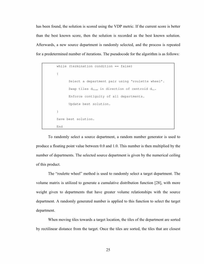
has been found, the solution is scored using the VDP metric. If the current score is better

than the best known score, then the solution is recorded as the best known solution.

Afterwards, a new source department is randomly selected, and the process is repeated

for a predetermined number of iterations. The pseudocode for the algorithm is as follows:

To randomly select a source department, a random number generator is used to

produce a floating point value between 0.0 and 1.0. This number is then multiplied by the

number of departments. The selected source department is given by the numerical ceiling

of this product.

The “roulette wheel” method is used to randomly select a target department. The

volume matrix is utilized to generate a cumulative distribution function [28], with more

weight given to departments that have greater volume relationships with the source

department. A randomly generated number is applied to this function to select the target

department.

When moving tiles towards a target location, the tiles of the department are sorted

by rectilinear distance from the target. Once the tiles are sorted, the tiles that are closest

while (termination condition == false)

{

Select a department pair using “roulette wheel”.

Swap tiles dfrom in direction of centroid dto.

Enforce contiguity of all departments.

Update best solution.

}

Save best solution.

End

26

to the target are allowed to move first. Moving the closer tiles first allows the tiles to

reduce the chance of swapping locations with tiles from their own department. If two tiles

are currently adjacent and elect to move in the same general direction, the prioritization

of moving the closer tile first allows the closer tile to move away from the other tile. This

makes it more likely that the other tile swaps locations with a tile that does not belong to

the same department.

Contiguity of a department is tested by selecting an arbitrary tile from a

department and building a spanning tree of tiles in its department. A tile is added to the

spanning tree if it is a neighbor of a current element in the spanning tree that is also in the

same department. If the spanning tree finds all tiles in its department, then the department

is deemed to be contiguous.

Contiguity is eventually guaranteed by following a diverse set of paradigms that

provided alternative pathways for the algorithm to avoid getting stuck in a stale search

space. SOT uses the following three paradigms:

• Tiles of divided departments move towards their own department centroid

• Tiles of the most severe department move towards their own centroid

• Department pairs are probabilistically selected based on their impact on

the overall VDP metric. Tiles of the selected deptfrom move towards the

centroid of the selected deptto.

Occasionally, the layout swarm will find itself in a situation where a tile swap will

divide a contiguous department to make another department contiguous, and a reversed

action would cause the newly contiguous department to become divided. For such a case,

27

the swarm must realize that it is in a stale search space, and switch to a alternative

pathway.

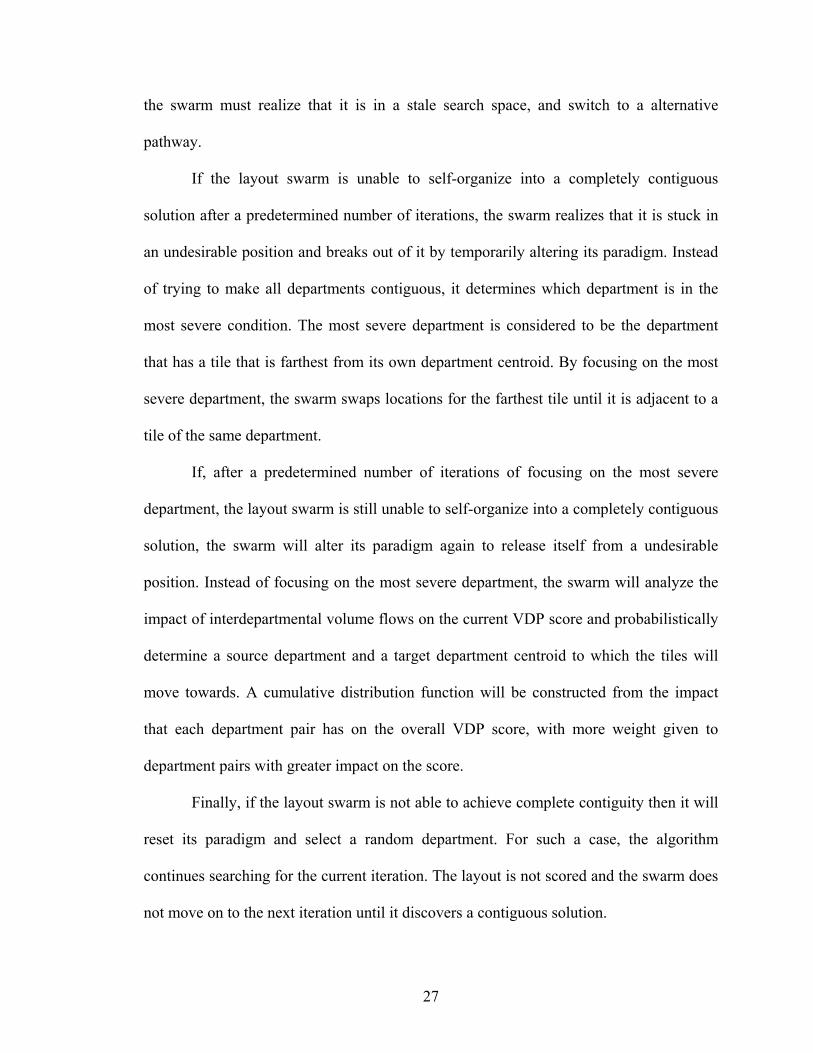
If the layout swarm is unable to self-organize into a completely contiguous

solution after a predetermined number of iterations, the swarm realizes that it is stuck in

an undesirable position and breaks out of it by temporarily altering its paradigm. Instead

of trying to make all departments contiguous, it determines which department is in the

most severe condition. The most severe department is considered to be the department

that has a tile that is farthest from its own department centroid. By focusing on the most

severe department, the swarm swaps locations for the farthest tile until it is adjacent to a

tile of the same department.

If, after a predetermined number of iterations of focusing on the most severe

department, the layout swarm is still unable to self-organize into a completely contiguous

solution, the swarm will alter its paradigm again to release itself from a undesirable

position. Instead of focusing on the most severe department, the swarm will analyze the

impact of interdepartmental volume flows on the current VDP score and probabilistically

determine a source department and a target department centroid to which the tiles will

move towards. A cumulative distribution function will be constructed from the impact

that each department pair has on the overall VDP score, with more weight given to

department pairs with greater impact on the score.

Finally, if the layout swarm is not able to achieve complete contiguity then it will

reset its paradigm and select a random department. For such a case, the algorithm

continues searching for the current iteration. The layout is not scored and the swarm does

not move on to the next iteration until it discovers a contiguous solution.

28

Once a contiguous solution is discovered, it is scored with the VDP metric. The

distance between two departments is calculated from the rectilinear distance between the

centroids of the departments. The interdepartmental flow is referenced from the volume

matrix. The cost value is referenced from the cost matrix.

Every time it finds a new score, its value is appended to a text file named

“scores.txt” that records the current score and the current best known score. If the current

score is the new best known score, then the current layout is also recorded to a file named

“bestN.txt”, where N is equal to the number of departments.

29

IV. RESULTS

Two data sets were created to test the performance of SOT. The first data set,

labeled T12, consists of a general layout for a 12-department facility. All of the

departments are of the same size. None of the departments have a fixed location

requirement. The floor plan of the facility is rectangular with a length-to-width ratio of

4:3. These dimensions were selected so that the single-tile representation of departments

would be able to fully occupy the layout space. This problem offers a level of

combinatorial complexity that is practically enumerable with a single-tile representation.

The second data set, labeled, T14, describes a layout with 14 departments. Two of

the departments have a fixed location requirement. All twelve of the non-fixed

departments have the same size. One of the fixed departments also has the same size as

the non-fixed departments; the other fixed department is twice as large as the rest of the

departments. The floor plan of the facility is rectangular with a length-to-width ratio of

5:3. Even though this data set contains more departments than the first data set, the

combinatorial complexity required to fully enumerate all possible layouts with a single-

tile representation is equal to that of the first problem since they both describe 12

departments without a fixed location requirement. To determine the absolute best layout

score with single-tile departments, both problems will require 12! = 4.79 × 108

evaluations.

30

The volume matrices for both problems were generated to emulate a realistic

scenario in which departments have volume relationships with a subset of all departments.

In addition, volume relationships are not necessarily equivalent. With the considerations,

the volume matrix was designed such that approximately 75 of the flow values were zero

(which indicates a lack of volume flow between two departments). The remaining

approximately 25 percent of the values were randomly generated with a uniform

distribution between 100 and 1,000. Tables I and II show the volume matrices for data set

T12 and T14, respectively.

Both data sets treat all movement between departments equally. As a result, all

values of the cost matrix are set to the same unit-cost of one.

TABLE I. Volume matrix for data set T12

TO FROM D1 D2 D3 D4 D5 D6 D7 D8 D9 D10 D11 D12

D1 0 923 0 0 0 240 560 329 0 0 857 0D2 383 0 0 0 0 738 0 869 0 681 928 0D3 938 334 0 0 0 0 0 0 0 0 0 0D4 0 0 794 0 414 0 0 125 0 484 0 0D5 0 0 0 915 0 0 0 0 0 0 0 0D6 0 0 184 0 606 0 0 0 0 0 0 0D7 0 0 0 983 0 440 0 0 0 0 0 795D8 0 740 0 0 0 0 196 0 920 0 0 0D9 0 900 572 0 552 382 0 0 0 0 0 647

D10 0 361 994 0 0 0 0 875 195 0 0 0D11 0 0 0 0 988 0 0 0 264 0 0 891D12 0 0 0 193 0 0 0 0 0 0 0 0

31

TABLE II. Volume matrix for data set T14 TO FROM D1 D2 D3 D4 D5 D6 D7 D8 D9 D10 D11 D12 D13 D14

D1 0 436 0 0 0 984 213 0 0 0 0 0 322 935D2 0 0 0 0 0 0 0 756 730 0 0 0 691 0D3 821 0 0 0 0 0 0 0 0 0 222 0 0 861D4 0 0 0 0 0 0 954 0 0 0 636 0 0 0D5 263 0 0 0 0 0 0 0 0 0 0 0 657 0D6 572 0 0 0 0 0 674 0 0 0 375 0 753 777D7 0 0 0 392 0 519 0 0 243 481 234 0 0 0D8 0 129 127 239 0 225 0 0 0 0 0 0 132 0D9 0 0 0 0 0 380 0 163 0 0 661 0 0 0

D10 0 0 0 0 0 0 0 0 791 0 0 851 0 343D11 0 0 543 0 946 0 156 277 0 353 0 596 505 0D12 0 0 0 667 0 696 0 0 414 929 0 0 0 878D13 717 0 0 221 0 0 0 0 0 0 587 576 0 0D14 0 0 0 0 0 0 0 480 0 0 633 0 975 0

A. Phase I For the first phase of experimentation, the size of the departments was controlled.

All departments were of equal size and represented by a single tile. The purpose of this

phase was to examine how well SOT approaches the absolute optimal score for data sets

where complete enumeration of all possible layouts is non-trivial but feasible.

Since each department is represented by a single tile, all departments will always

be contiguous since they cannot be divided. Therefore, a new layout is produced every

time two tiles swap locations. For this experiment, 30 trials were run for 60,000 iterations

each. Results for the data set T12 is presented in Table III.

32

TABLE III. Results for data set T12, single tile per department

Complete Enumeration SOT

Iterations 479,001,600 60,000

Runtime 2,269 minutes 1.37 minutes (average)

Best Score 36,949 37,028

Worst Score 71,928 68,061

Average Score 54,110 51,995

Standard Deviation 3,782 3,630

Scores for SOT solutions to the T12 data set ranged between 37,028 and 68,061.

The best score encountered was very considerably close to the absolute optimal score of

36,949. A histogram of scores is presented in Figure 8, which reveals that the scores are

normally distributed. The best solution discovered by SOT after 60,000 iterations missed

the absolute optimal score by 79 points—0.2 percent of the enumerated range. The

performance of SOT after 60,000 iterations is promising considering complete

enumeration required the evaluation of all 12! = 4.79 × 108 possible layouts.

33

0

500

1000

1500

2000

2500

3000

3500

3650

0

3850

0

4050

0

4250

0

4450

0

4650

0

4850

0

5050

0

5250

0

5450

0

5650

0

5850

0

6050

0

6250

064

500

6650

0

6850

0

7100

0

VDP Score

Num

ber

of O

ccur

renc

es

SOT Enum

FIGURE 8. VDP Histogram for SOT (single tile), enumeration (normalized to SOT) on T12 data set

Results for the data set T14 is presented in Table IV. Scores for SOT solutions to

the T14 data set ranged between 55,404.5 and 95,205.5. The best score encountered was

very considerably close to the absolute optimal score of 50,243. A normally distributed

histogram of scores is presented in Figure 9. The best solution discovered by SOT after

60,000 iterations missed the absolute optimal score by 5,161.5 points—11.6 percent of

the enumerated range. While there is still room for improvement, this illustrates the

effectiveness of the SOT approach since less than 0.1% of all possible solutions are

explored.

34

TABLE IV. Results for data set T14, 1 tile per department

Complete Enumeration SOT

Iterations 479,001,600 60,000

Runtime 2845 minutes 1.43 minutes (average)

Best Score 50,243 55,404.5

Worst Score 94,802 95,205.5

Average Score 71,319.2 74,266.8

Standard Deviation 4,582.3 4,530.3

0

200

400

600

800

1000

1200

1400

5000

052

500

5500

057

500

6000

062

500

6500

067

500

7000

072

500

7500

077

500

8000

082

500

8500

087

500

9000

092

500

VDP Score

Num

ber o

f Occ

urre

nces

SOT Enum

FIGURE 9. VDP Histogram for SOT (single tile), enumeration (normalized to SOT) on T14 data set

35

B. Phase II

For the second phase of experimentation, the size of the departments was

controlled. All departments were of equal size and represented by four tiles. The purpose

of this phase was to examine the effect of granularity on the performance of SOT.

Since each department is represented by a multiple tiles, departments can be

divided and will not always be contiguous. Unlike the single-tile representation, a new

layout (with completely contiguous departments) is not usually produced every time two

tiles swap locations. For this experiment, 30 trials were run for 20,000 iterations each.

Results for the data set T12 is presented in Table V. Scores for SOT solutions to

the T12 data set ranged between 78,789.5 and 132,985.5. A histogram of scores is

presented in Figure 10 to reveal a generally normal distribution.

TABLE V. Results for data set T12, four tiles per department

Iterations 20,000

Average Runtime 222.09 seconds

Best Score 78,789.5

Worst Score 132,985.5

Average Score 104,072.1

Standard Deviation 6,830.2

Scores for layouts where all departments are represented by multiple tiles can be

normalized for comparison with scores for layouts with single-tile departments. The

normalization factor is obtained by comparing the scores of equivalent layouts. To

36

achieve equivalent layouts with four tiles per department, a single-tile department is

divided into a 2x2 grid array of tiles. As a result, rectilinear distance between centroids is

doubled, so the scores are generally twice that of their single-tile representations.

0

100

200

300

400

500

600

7650

0

8000

0

8350

0

8700

0

9050

0

9400

0

9750

0

1010

00

1045

00

1080

00

1115

00

1150

00

1185

00

1220

00

1255

00

1290

00

1325

00

VDP Score

Num

ber o

f Occ

urre

nces

FIGURE 10. VDP Histogram for SOT (four tiles per department) on T12 data set

Results for the data set T14 is presented in Table VI. Scores for SOT solutions to

the T14 data set ranged between 108,020.3 and 172,047.3. A histogram of scores is

presented in Figure 11, displaying a normal distribution.

37

TABLE VI. Results for data set T14, 4 tiles per department

Iterations 20,000


Best Score 108,020.3


Average Score 132,458


0

100

200

300

400

500

600

700

1080

00

1115

0011

5000

1185

00

1220

0012

5500

1290

00

1325

00

1360

0013

9500

1430

00

1465

0015

0000

1535

00

1570

00

1605

0016

4000

1675

00

1710

00

VDP Score

Num

ber o

f Occ

uren

ces

FIGURE 11. VDP Histogram for SOT (four tiles per department) on T14 data set

Further investigation of the effect of granularity was performed by evaluating the

performance when all departments are represented by nine tiles. To achieve equivalent

38

layouts with nine tiles per department, a single-tile department is divided into a 3x3 grid

array of tiles.

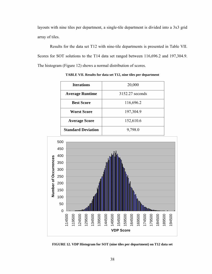
Results for the data set T12 with nine-tile departments is presented in Table VII.

Scores for SOT solutions to the T14 data set ranged between 116,696.2 and 197,304.9.

The histogram (Figure 12) shows a normal distribution of scores.

TABLE VII. Results for data set T12, nine tiles per department

Iterations 20,000




Average Score 152,610.6


0

50

100

150

200

250

300

350

400

450

500

1145

00

1195

00

1245

00

1295

00

1345

00

1395

00

1445

00

1495

00

1545

00

1595

00

1645

00

1695

00

1745

00

1795

00

1845

00

1895

00

1945

00

VDP Score

Num

ber o

f Occ

urre

nces

FIGURE 12. VDP Histogram for SOT (nine tiles per department) on T12 data set

39

Results for the data set T14 with nine-tile departments is presented in Table VIII.

Scores for SOT solutions to the T14 data set ranged between 37,028 and 68,061. A

histogram of scores is presented in Figure 13.

TABLE VIII. Results for data set T14, nine tiles per department

Iterations 20,000




Average Score 132,458


0

100

200

300

400

500

600

700

800

900

1590

00

1650

00

1710

00

1770

00

1830

00

1890

00

1950

00

2010

00

2070

00

2130

00

2190

00

2250

00

2310

00

2370

00

2430

00

2490

00

VDP Score

Num

ber o

f Occ

urre

nces

FIGURE 13. VDP Histogram for SOT (nine tiles per department) on T14 data set

40

Finally, the Pearson product-moment correlation coefficient was measured for the

relationship between best known scores of the initial iteration and of the last iteration.

The degree of correlation was measured to test whether an initial iteration with a low

score would a yield lower score for the last iteration than if the initial iteration had a

higher score. Such a correlation would suggest that the algorithm continuously improves

upon good solutions. The results of the correlation measurements are presented in Table

IX

.

TABLE IX. Pearson correlation coefficient for best known score of initial and last iteration

Data Set Granularity

(Tiles per department)

Pearson correlation

coefficient

1 0.3576

4 0.0750 T12

9 0.1749

1 0.0269

4 0.0837 T14

9 -0.0312

A Pearson correlation coefficient of 1.000 would indicate an increasing linear

relationship, while a correlation coefficient of −1.000 would indicate decreasing linear

relationship. With correlation coefficients close to zero, the overall results indicate a very

weak correlation between initial and last iterations of a trial. The results demonstrate that

the score of the last iteration is independent of the score of the initial iteration. The

randomness of the algorithm enables the solution space to be independent of the starting

condition.

41

C. Phase III

The CRAFT algorithm [19] is a widely used method to design a facility layout.

Since CRAFT is a deterministic algorithm, it will generate the same solution for a given

input. As a result, it requires a feasible solution to provide an initial state. Using two

datasets from DePuy and Usher [29], Hardin and Usher [2] demonstrated that their

Layout Swarm could improve upon CRAFT’s performance. Using the same datasets, the

performance of SOT was compared with Layout Swarm. Results are presented in Table X.

TABLE X.Comparison of Results of SOT with Layout Swarm and CRAFT

Best VDP Score Found Data Set [29]

SOT Layout Swarm CRAFT

M11 1,386 1,378 1,368

M15 32,727 32,752 34,301

The results of SOT and Layout Swarm are essentially the same for both datasets.

VDP scores for SOT typically ranged from 32,000 to 36,000—the same as Layout

Swarm. It may not be a significant improvement over Layout Swarm, but it is worth

noting that SOT found a better layout than previously discovered.

D. Phase IV

For this experiment, the quality of the best layouts produced from the previous

phases were analyzed by applying shape measures introduced by Bozer et al. [3]. The

results of the analysis are presented in Table XI.

42

TABLE XI. Calculated Shape Measures for Layouts with Best Scores

Data Set Granularity

(Tiles per department) Average Ω value

1 1.000

4 1.210 T12

9 1.356

1 1.000

4 1.178 T14

9 1.316

The average Ω value of the layout increased as department granularity was

increased. When departments are represented by a single tile, then their Ω values are

always 1.000 because a single tile has a perfectly regular shape. As greater granularity is

applied to department representation, the average Ω value increases because the

department has increased potential to have irregular shapes. Increasing granularity from

one to four tiles per department cause a 19.4 percent increase in average Ω value, and a

33.6 percent increase for 9 tiles per department. The average values remained below 1.50,

the suggested upper limit for reasonable shapes [3], and so the shapes of the layouts

produced by SOT were generally acceptable when departments were represented by one,

four, or nine tiles.

43

V. DISCUSSION

The robustness and adaptability of the swarm lends itself towards the need to

further evaluate performance in a multitude of scenarios and problems, especially the

ones that have greater combinatorial complexity than the problems described by the

examined data sets. With more time, the swarm may be able to discover solutions with

better and better scores. Future investigation would allow SOT to continue to run for

more and more iterations with the prospect of finding better and better solutions.

Further development of the using swarm intelligence as a tool to find facility

layout solutions would involve incorporating flexibility that would allow it to be applied

to practical facility layout planning beyond rectangular floor plans.

The results demonstrated that increased granularity of a department allows it

deteriorate into a less regular shape. The issue of irregular department shapes needs to be

addressed, especially if departments are to be represented by a large number of tiles.

Future research will involve studying ways to incorporate alternative metrics such

as shape measures into the social information passed around within the particle swarm of

tiles. This would help the swarm to become self-aware of movement of tiles that would

deter the solution from having irregular-shaped departments. Decisions that result in a

unfavorable shapes should be penalized.

44

Future work could involve examining methods of transforming contiguous

departments into prescribed shapes. In addition, future work could examine pathways for

achieving contiguity for departments that this thesis introduced. If multiple pathways are

to be employed, future work could analyze the effect of various methods of prioritizing of

these pathways on the performance of SOT.

45

VI. CONCLUSION

Swarm intelligence is a practical method for solving facility layout problems with

high combinatorial complexity. Rather than employ an explicit objective function, the

swarm paradigm generates solutions through emergent behavior. The behavior emerges

as tiles swap locations with neighbors only by following a simple set of rules. The

objective is implied by the rules.

The aim of this thesis was to evaluate swarm intelligence as a viable

computational tool for solving facility layout problems and to assess the quality of

discovered solutions using a shape measure. This thesis accomplished several tasks.

The major achievement of this thesis was the design and implementation of a tool

that could produce facility layout solutions using Self-Organizing Tiles (SOT). During

the design of the tool, this thesis advanced the swarm paradigm by introducing alternative

pathways for achieving contiguity of departments.

This thesis utilized the tool to examine the convergence of SOT on an enumerated

optimum for a layout dataset, which required the exhaustive evaluation of all

permutations of a grid layout. SOT was found to approach the enumerated optimal score

within 0.2 percent of the range of all possible scores for T12 and 11.6 percent of the

range of all possible scores for T14. The tool was also used to examine the effect of

granularity on the ability of SOT to converge on facility layout solutions, and found

similar performance. A shape metric was utilized as a means of evaluating the quality of

46

produced solutions based on the regularity of the shape of departments, and found that

SOT produces fairly regular layouts when granularized to nine tiles per department. The

overall regularity of departments is a fair indicator of the practicality of implementing the

solution. Finally, SOT was compared with other algorithms the experimental results

revealed that SOT performed similarly and with minor improvements to Hardin and

Usher’s implementation of the Layout Swarm, which had already provided improvements

over the CRAFT algorithm.

47

REFERENCES

[1] A. Kusiak and S. S. Heragu, "The Facility Layout Problem," European Journal of Operational Research, vol. 29, no. 3, pp. 229-251, June1987.

[2] C. T. Hardin and J. S. Usher, "Facility Layout Using Swarm Intelligence," IEEE Press, 2005.

[3] Y. A. Bozer, R. D. Meller, and S. J. Erlebacher, "Improvement-type layout algorithm for single and multiple-floor facilities," Management Science, vol. 40, no. 7, pp. 918-932, 1994.

[4] R. G. Askin and C. R. Stanridge, Modeling and Analysis of Manufacturing Systems 1993, pp. 204-253.

[5] A. R. J. McKendall, J. S. Noble, and C. M. Klein, "Facility Layout of Irregular-Shaped Departments Using a Nested Approach," International Journal of Production Research, vol. 37, no. 13, pp. 2895-2914, 1999.

[6] J. C. Mecklenburgh, Process Plant Layout. New York: Halstead Press, 1985.

[7] R. L. Francis, L. F. McGinnis, and J. A. White, Facility Layout and Location: An Analytical Approach (2nd Ed). Englewood Cliffs, NJ: Prentice Hall, 1992, pp. 27-171.

[8] J. A. Tompkins, J. A. White, Y. A. Bozer, E. H. Frazelle, J. M. Tanchoco, and J. Trevino, Facilites Planning, 2nd ed. New York: John Wiley and Sons, 1996.

[9] D. M. Tate and A. E. Smith, "Genetic Algorithm Optimization Applied to Variations of the Unequal Area Facilities Layout Problem," Proceedings of the 2nd Industrial Engineering Research Conference, pp. 335-339, 1993.

[10] R. D. Meller and K.-Y. Gau, "The Facility Layout Problem: Recent and Emerging Trends and Perspectives," Journal of Manufacturing Systems, vol. 15, no. 5, pp. 351-366, 1996.

[11] V. S. Sheth, Facilities Planning and Materials Handling: Methods and Requirements. New York: Marcel Dekker, Inc., 1995, pp. 67-86.

[12] T. C. Koopmans and M. Beckmann, "Assignment Problems and the Location of Economic Activities," Econometrica, vol. 25, no. 1, pp. 53-76, Jan.1957.

[13] P. C. Gilmore, "Optimal and Suboptimal Algorithms for the Quadratic Assignment Problem," Journal of the Society for Industrial and Applied Mathematics, vol. 10, pp. 305-313, 1962.

48

[14] E. L. Lawler, "The Quadratic Assignment Problem," Management Science, vol. 9, no. 4, pp. 586-599, July1963.

[15] S. Sahni and T. Gonzalez, "P-Complete Approximation Problems," Journal of the ACM, vol. 23, no. 3, pp. 555-565, July1976.

[16] T. W. Liao, "Design of the Line Type Cellular Manufacturing Systems for Minimum Operating and Total Material Handling Costs," International Journal of Production Research, vol. 32, no. 2, pp. 387-397, 1993.

[17] B. Montreuil, "A modeling framework for integrating layout design and flow network design," Proc. of the Material Handling Research Colloquium, Hebron, KY, pp. 43-58, 1990.

[18] S. S. Heragu and A. Kusiak, "Efficient models for the facility layout problem," European Journal of Operational Research, vol. 53, no. 1, pp. 1-13, July1991.

[19] G. C. Armour and E. S. Buffa, "Heuristic algorithm and simulation approach to relative location of facilities," Management Science, vol. 9, pp. 294-309, 1963.

[20] R. C. Lee and J. M. Moore, "CORELAP - computerized realtionship layout planning," Journal of Industrial Engineering, vol. 18, pp. 195-200, 1967.

[21] M. Goetschalckx, "Interactive layout heuristic based on hexagonal adjacency graphs," European Journal of Operational Research, vol. 63, no. 2, pp. 304-321, 1992.

[22] L. R. Foulds and D. F. Robinson, "A Strategy for Solving the Plant Layout Problem," Operations Research Quarterly, vol. 27, no. 4, pp. 845-855, 1976.

[23] M. S. Bazaraa and M. D. Sherali, "Benders' Partitioning Scheme Applied to a New Formulation of the Quadratic Assignment Problem," Naval Resarch Logistics Quarterly, vol. 27, no. 1, pp. 29-41, 1980.

[24] R. S. Liggett and W. J. Mitchell, "Optimal Space Planning in Practice," Computer-Aided Design, vol. 13, no. 5, pp. 277-288, 1981.

[25] H. Freeman, "Computer Processing of Line-Drawing Images," ACM Computing Surveys, vol. 6, no. 1, pp. 57-97, 2007.

[26] J. Kennedy and R. Eberhart, "Particle swarm optimization," in Proceedings IEEE International Conference on Neural Networks, 1995 (Perth, Austraila), 4 ed 1995, pp. 1942-1948.

[27] M. Mitchell, An Introduction to Genetic Algorithms. Cambridge, Massachusetts: The MIT Press, 1996, pp. 166-167.

49

[28] J. Banks, J. S. Carson III, B. L. Nelson, and D. M. Nicol, Discrete-Event System Simulation, 4th ed. Upper Saddle River, NJ: Pearson Education Inc., 2005, pp. 153-154.

[29] G. W. DePuy, J. S. Usher, and T. J. Miles, "Facilities Layout Using CRAFT Meta-Heuristic," in Proceedings of the Industrial Engineering Research Conference 2004.

50

APPENDIX I

LIST OF ABBREVIATIONS

PSO Particle Swarm Optimization

SOT Self-Organizing Tiles

VDP Volume-Distance Product

WIP work-in-process

I/O input/output

CTC centroid-to-centroid

QAP Quadratic Assignment Problem

MIP Mixed-Integer Programming

51

CURRICULUM VITAE

ANDREW BAO THAI

Date of Birth February 28, 1984

Place of Birth Louisville, Kentucky

Undergraduate Study University of Louisville


2002-2006

Graduate Study University of Louisville


2006-2007

Experience Course Lecturer, University of Louisville

(January 2007 – May 2007)

Student System Administrator, University of Louisville

(August 2006 – March 2007)

Student Assistant, University of Louisville

(January 2006 – August 2006)

Applications Support and Development Co-op,

UPS Airlines – Louisville, Kentucky

(January 2004 – August 2005)

EVALUATION OF USING SWARM INTELLIGENCE TO PRODUCE FACILITY...

Documents

Transcript of EVALUATION OF USING SWARM INTELLIGENCE TO PRODUCE FACILITY...