1

Evaluation of the WRF PBL parameterizations for marine boundary layer clouds: Cumulus and stratocumulus

Hsin-Yuan Huang1, Alex Hall2, and Joao Teixeira3

1Joint Institute for Regional Earth System Science and Engineering, University of California, Los Angeles

2Department of Atmospheric and Oceanic Sciences, University of California, Los Angeles

3Jet Propulsion Laboratory, California Institute of Technology

Submitted to: Monthly Weather Review (Expedited Contribution)

Revised manuscript submitted on: 01/11/2013

____________________ Corresponding author address: Hsin-Yuan Huang, 7343 Math Science Building, University of California, Los Angeles E-mail: hyhuang@ucla.edu

2

Abstract 1

The performance of five boundary layer parameterizations in the Weather 2

Research and Forecasting model is examined for marine boundary layer cloud regions 3

using a single column model version of the WRF model. Most parameterizations show a 4

poor agreement of the vertical boundary layer structure when compared with Large-Eddy 5

Simulation models. These comparisons against Large-Eddy Simulation show that a 6

parameterization based on the Eddy-Diffusivity/Mass-Flux approach provides a better 7

performance. The results also illustrate the key role of boundary layer parameterizations 8

in model performance. 9

10

1. Introduction 11

Stratocumulus and shallow cumulus clouds in subtropical oceanic regions cover 12

thousands of square kilometers and play a key role in regulating global climate (e.g. 13

Tiedtke et al., 1988; Klein and Hartmann, 1993). Stratocumulus cools the climate by 14

strongly reflecting incoming shortwave radiation, playing an important role in ocean-15

atmosphere interaction (e.g. Teixeira et al., 2008), while cumulus clouds play a key role 16

in regulating the planet’s evaporation and moisture transport to the deep tropics. 17

Numerical modeling is an essential tool to study these clouds in regional and global 18

systems, but the current generation of climate and weather models has difficulties in 19

representing them in a realistic way. Stratocumulus boundary layers in models are often 20

unrealistically shallow and have too little cloud (e.g. Duynkerke and Teixeira, 2001; 21

Zhang et al., 2005; Stevens et al., 2007). Additionally, current models have difficulties in 22

3

simulating the critical transition from stratocumulus to shallow cumulus clouds 23

(Siebesma et al., 2004; Teixeira et al., 2011). 24

While numerical models resolve the large-scale flow, subgrid-scale 25

parameterizations are needed to estimate small-scale properties (e.g. boundary layer 26

turbulence and convection, clouds, radiation), which have significant influence on the 27

resolved scale due to the complex nonlinear nature of the atmosphere. For the cloudy 28

planetary boundary layer (PBL), it is fundamental to parameterize vertical turbulent 29

fluxes and subgrid-scale condensation in a realistic manner. The Weather Research and 30

Forecasting (WRF) model version 3.1 provides multiple parameterization choices, which 31

include nine PBL schemes, 12 microphysics and six moist convection parameterizations 32

(Skamarock et al., 2008). In addition to a typical model structural drawback – an artificial 33

separation between turbulence and convection parameterizations, this long menu suffers 34

from a variety of issues including an uncertainty regarding the optimal combinations to 35

select. 36

In this study, we aim to investigate the performance of the various WRF PBL 37

schemes in cloud simulations of both marine stratocumulus and shallow cumulus. 38

Meanwhile, we also evaluate the ability of a new scheme (TEMF, described below) based 39

on the Eddy-Diffusivity/Mass-Flux (EDMF) concepts. We design a set of several WRF 40

single column model (SCM) simulations for three well-known Large-Eddy Simulation 41

(LES) case-studies based on field campaigns. Including the TEMF scheme, five PBL 42

parameterizations are examined against LES. Resolving the large eddies which are 43

responsible for the transport of mass, momentum and energy in the PBL, LES result has 44

been used to serve as a proxy of reality to guide the development of PBL 45

4

parameterization. Section 2 briefly introduces the EDMF and TEMF schemes. Section 3 46

describes the experimental design. Section 4 presents the simulation results followed by a 47

discussion in Section 5. 48

49

2. EDMF and TEMF parameterizations 50

The EDMF parameterization was first introduced by Siebesma and Teixeira 51

(2000) and subsequently tested and implemented in the European Centre for Medium-52

range Weather Forecasts (ECMWF) model (e.g. Teixeira and Siebesma, 2000; Koehler, 53

2005). Recent studies have shown its potential to represent the shallow and dry 54

convective PBL (Soares et al., 2004; Siebesma et al., 2007; Neggers, 2009; Witek et al., 55

2011; Suselj et al., 2012). Later, using total turbulent energy to calculate eddy-diffusivity 56

(Mauritsen et al., 2007), Angevine et al. (2010) modified the EDMF parameterization to 57

what is referred to as the Total-Energy/Mass-Flux (TEMF) parameterization. The TEMF 58

scheme implemented in WRF version 3.1 is evaluated in this study. 59

Rather than a specific parameterization, EDMF is an approach based on an 60

optimal combination of the eddy-diffusivity (ED) parameterization, used to simulate 61

turbulence within the PBL, and the mass-flux (MF) parameterization, used for moist 62

convection. Though differences in the details are present in different EDMF 63

implementations on weather or climate models, the fundamental idea is the same: Local 64

mixing is parameterized by the ED term, while the non-local transport due to convective 65

thermals is represented by the MF term. The governing equation for the vertical fluxes in 66

EDMF is: 67

( )upw K Mzψψ ψ ψ∂′ ′ = − + −∂

, (1) 68

5

where ψ can be any scalar quantity, such as liquid water potential temperature ( lθ ), total 69

water specific humidity ( tq ), or total energy ( E ). K and M are the ED and MF terms, 70

respectively; the subscript up in upψ indicates the value of ψ in the updraft. The 71

temporal evolution of the mean variable ψ is then given as the vertical gradient of the 72

flux: ( )t w zψ ψ′ ′∂ ∂ = −∂ ∂ . 73

The main difference between TEMF and EDMF is in the calculation of the ED 74

coefficient: EDMF often uses turbulent kinetic energy (TKE) while TEMF uses total 75

turbulent energy (TTE), a combination of TKE and turbulent potential energy. Better 76

handling of stably-stratified conditions is the main reason for using TTE rather than TKE 77

(Mauritsen et al., 2007). For a full description of TEMF, the reader is referred to 78

Angevine (2005), Mauritsen et al. (2007), Siebesma et al. (2007), and Angevine et al. 79

(2010). 80

81

3. Experimental design 82

3.1 Study sites 83

We perform a suite of simulations using the SCM version of WRF for 3 case-84

studies associated with field experiments, which are chosen because they have been 85

intensively studied using LES models. The three field campaigns are: 1) the second 86

Dynamics and Chemistry of Marine Stratocumulus (DYCOMS-II) field study, 2) the 87

Barbados Oceanographic and Meteorological Experiment (BOMEX), and 3) the Rain in 88

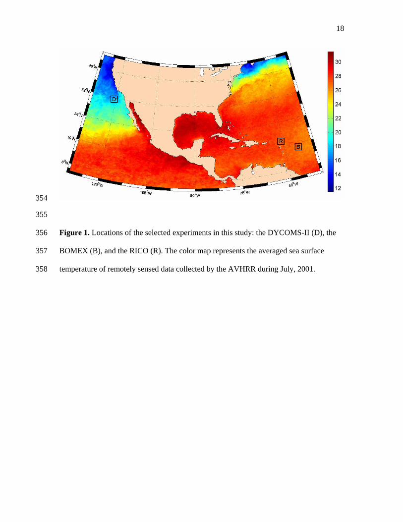
Cumulus over Ocean (RICO) experiment (Fig. 1). DYCOMS- II took place in the 89

subtropical Pacific, while BOMEX and RICO were in the tropical Atlantic. The marine 90

clouds in BOMEX and RICO are classified as shallow cumulus while the DYCOMS-II 91

6

case is classified as stratocumulus. DYCOMS-II was conducted in the center of the 92

Northeast Pacific stratocumulus deck, about 500 km west-southwest of San Diego, 93

California, during July 2001 (Stevens et al., 2003; Stevens et al., 2005). The first 94

Research Flight mission of DYCOMS-II is selected for this study because it provides 95

many appropriate atmospheric conditions for the LES experiment, such as a relatively 96

homogeneous atmospheric environment and a uniform cloud distribution. BOMEX 97

(Phase III) took place during June 1969 over a 500 km2 region near Barbados. The aim 98

was to investigate the large-scale heat and moisture budgets using radiosondes (Delnore, 99

1972; Holland and Rasmusson, 1973). In this study, the SCM setup and initialization for 100

BOMEX use the same settings as previous LES studies (e.g. Siebesma and Cuijpers, 101

1995; Siebesma et al., 2003). RICO was carried out near the Caribbean islands during a 102

two-month period between November 2004 and January 2005 (Caesar, 2005; Rauber et 103

al., 2007). Here the SCM initialization for RICO follows the designs of an LES 104

intercomparison study presented in the 9th GCSS boundary layer cloud workshopa. All 105

LES ensemble results (for three study sites) shown in the following analyses are taken 106

from these intercomparison studies. 107

3.2 Single-column model setup 108

This study uses WRF version 3.1 for all SCM experiments. In addition to TEMF, 109

four other PBL schemes are used: the Yonsei University (YSU) scheme (Hong et al., 110

2006), the Mellor-Yamada-Janjic (MYJ) scheme (Mellor and Yamada, 1982; Janjic, 111

2002), the Mellor-Yamada-Nakanishi-Niino (MYNN) scheme (Nakanishi and Niino, 112

2004, 2006), and the Medium Range Forecast (MRF) scheme (Hong and Pan, 1996). 113

Note that YSU and MRF are classified as first-order schemes while the others are TKE 114 a http://www.knmi.nl/samenw/rico/index.html

7

closure schemes, where a prognostic TKE equation is used to determine the eddy 115

diffusivity. All PBL schemes used in this study are listed in Table 1. In addition, a moist 116

convection parameterization, the Kain-Fritsch scheme (Kain and Fritsch, 1993; Kain, 117

2004), is selected for the non-TEMF SCM simulations of the BOMEX and RICO cases. 118

This allows us to compare the results using the existing WRF PBL schemes with TEMF 119

for shallow cumulus cases. The TEMF code used in WRF version 3.1 was a pre-released 120

version, TEMF was not released until version 3.3. However, the two versions are similar. 121

In WRF, the cloud microphysics component estimates the amount of various 122

types of condensed water (i.e. cloud, rain, and ice). Thus, for a given WRF PBL scheme, 123

the estimated cloud liquid water can vary with the choice of microphysics scheme. For 124

each PBL scheme used in this study, we perform nine simulations with each of the nine 125

available microphysics schemes, also listed in Table 1. However, because of the 126

qualitative similarity of the vertical profile shapes across microphysics schemes, the 127

average over the ensembles of simulations using the various microphysics schemes is 128

presented. The vertical domain of the SCM experiments includes 116 levels up to an 129

altitude of 12000 m and the simulation timestep is 30 seconds. Other model setups are 130

consistent with previous LES intercomparison studies. 131

132

4. Results 133

Vertical profiles of the temperature and water content variables are illustrated in 134

the following figures to compare temporally-averaged SCM estimates and the LES 135

results for DYCOMS-II (Fig. 2), BOMEX (Fig. 3) and RICO (Fig. 4) cases. In each 136

subplot, shaded areas and black dashed lines represent the range of output of the LES 137

8

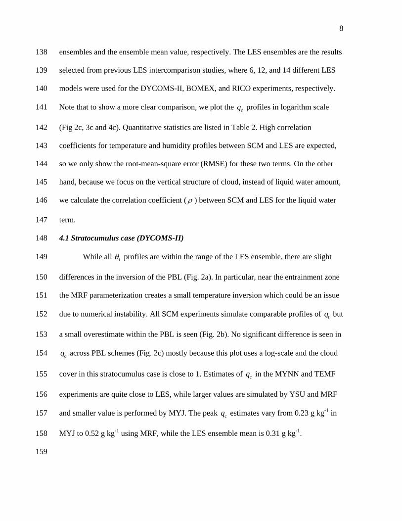
ensembles and the ensemble mean value, respectively. The LES ensembles are the results 138

selected from previous LES intercomparison studies, where 6, 12, and 14 different LES 139

models were used for the DYCOMS-II, BOMEX, and RICO experiments, respectively. 140

Note that to show a more clear comparison, we plot the cq profiles in logarithm scale 141

(Fig 2c, 3c and 4c). Quantitative statistics are listed in Table 2. High correlation 142

coefficients for temperature and humidity profiles between SCM and LES are expected, 143

so we only show the root-mean-square error (RMSE) for these two terms. On the other 144

hand, because we focus on the vertical structure of cloud, instead of liquid water amount, 145

we calculate the correlation coefficient ( ρ ) between SCM and LES for the liquid water 146

term. 147

4.1 Stratocumulus case (DYCOMS-II) 148

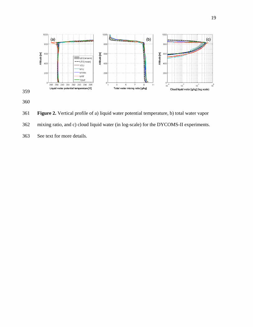
While all lθ profiles are within the range of the LES ensemble, there are slight 149

differences in the inversion of the PBL (Fig. 2a). In particular, near the entrainment zone 150

the MRF parameterization creates a small temperature inversion which could be an issue 151

due to numerical instability. All SCM experiments simulate comparable profiles of tq but 152

a small overestimate within the PBL is seen (Fig. 2b). No significant difference is seen in 153

cq across PBL schemes (Fig. 2c) mostly because this plot uses a log-scale and the cloud 154

cover in this stratocumulus case is close to 1. Estimates of cq in the MYNN and TEMF 155

experiments are quite close to LES, while larger values are simulated by YSU and MRF 156

and smaller value is performed by MYJ. The peak cq estimates vary from 0.23 g kg-1 in 157

MYJ to 0.52 g kg-1 using MRF, while the LES ensemble mean is 0.31 g kg-1. 158

159

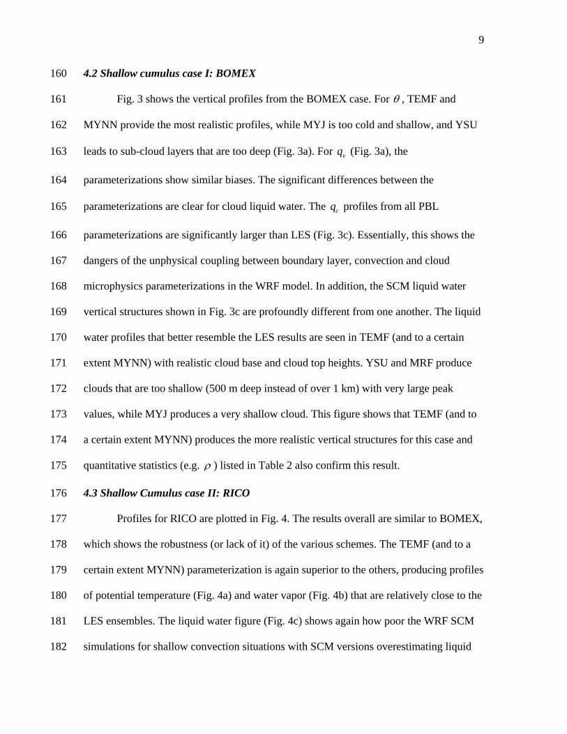
9

4.2 Shallow cumulus case I: BOMEX 160

Fig. 3 shows the vertical profiles from the BOMEX case. For θ , TEMF and 161

MYNN provide the most realistic profiles, while MYJ is too cold and shallow, and YSU 162

leads to sub-cloud layers that are too deep (Fig. 3a). For vq (Fig. 3a), the 163

parameterizations show similar biases. The significant differences between the 164

parameterizations are clear for cloud liquid water. The cq profiles from all PBL 165

parameterizations are significantly larger than LES (Fig. 3c). Essentially, this shows the 166

dangers of the unphysical coupling between boundary layer, convection and cloud 167

microphysics parameterizations in the WRF model. In addition, the SCM liquid water 168

vertical structures shown in Fig. 3c are profoundly different from one another. The liquid 169

water profiles that better resemble the LES results are seen in TEMF (and to a certain 170

extent MYNN) with realistic cloud base and cloud top heights. YSU and MRF produce 171

clouds that are too shallow (500 m deep instead of over 1 km) with very large peak 172

values, while MYJ produces a very shallow cloud. This figure shows that TEMF (and to 173

a certain extent MYNN) produces the more realistic vertical structures for this case and 174

quantitative statistics (e.g. ρ ) listed in Table 2 also confirm this result. 175

4.3 Shallow Cumulus case II: RICO 176

Profiles for RICO are plotted in Fig. 4. The results overall are similar to BOMEX, 177

which shows the robustness (or lack of it) of the various schemes. The TEMF (and to a 178

certain extent MYNN) parameterization is again superior to the others, producing profiles 179

of potential temperature (Fig. 4a) and water vapor (Fig. 4b) that are relatively close to the 180

LES ensembles. The liquid water figure (Fig. 4c) shows again how poor the WRF SCM 181

simulations for shallow convection situations with SCM versions overestimating liquid 182

10

water by about one order of magnitude. TEMF shows a vertical structure of liquid water 183

that although overestimating the overall values (as for all other parameterizations) 184

produces realistic cloud base and cloud top heights. YSU and MRF produce again clouds 185

that are quite shallow (around 500 m deep versus 2 km for the LES) and MYJ produces 186

even shallower (and lower) clouds. Table 2 also illustrates that the vertical cloud 187

structures from the MYNN and TEMF experiments are the ones most close to LES. 188

189

5. Conclusions and Discussion 190

An intercomparison of five PBL parameterizations in the WRF model for marine 191

cloudy boundary layers is presented in this study. Four existing WRF PBL schemes and 192

the recently developed TEMF scheme (based on the EDMF approach) are evaluated for 193

their performance against LES results in terms of the vertical profiles of meteorological 194

states for one stratocumulus case and two shallow cumulus cases. 195

For the stratocumulus case there are some differences in the upper region of the 196

PBL with some parameterizations producing an artificial and noisy vertical structure in 197

potential temperature. In liquid water, all models produce a similar structure but with 198

some differences in terms of absolute values. For both shallow cumulus cases, the results 199

are fairly similar with TEMF, and to a certain extent MYNN, producing superior 200

depictions of the thermodynamical vertical structure. All SCMs clearly overestimate the 201

values of liquid water when compared to the LES results, mostly because of the 202

unphysical coupling between boundary layer and cloud microphysics parameterizations 203

in WRF. In spite of this large positive bias, the TEMF version produces realistic cloud 204

base and cloud heights for both BOMEX and RICO. Other parameterizations produce 205

11

cloud structures that are too shallow not resembling shallow cumulus boundary layers at 206

all in this context. 207

In spite of its simplicity, this study leads to some key general conclusions: 208

1) A parameterization based on the EDMF approach (i.e. TEMF) that unifies 209

different components (turbulence and moist convection) produces a better result 210

when compared with LES, with realistic vertical structures for stratocumulus and 211

cumulus regimes; 212

2) Existing PBL parameterizations in WRF are not able to produce fully realistic 213

results when simulating stratocumulus and shallow cumulus regimes; 214

3) The often artificial modularity of parameterizations as they are implemented in 215

WRF produces unreliable results that are virtually impossible to interpret due to 216

the plethora of available parameterizations and their coupling. 217

218

Acknowledgments. 219

This work was supported by the Department of Energy Grant #DE-SC0001467. The 220

authors thank Dr. Wayne Angevine at the National Oceanic and Atmospheric 221

Administration and Dr. Thorsten Mauritsen at the Max Planck Institute for Meteorology 222

for their invaluable discussions on this work. We also thank Dr. Joshua Hacker at the 223

Naval Postgraduate School for his help on WRF single-column model simulations. Help 224

and discussion from Dr. Kay Suselj at the Caltech Jet Propulsion Laboratory are also 225

greatly acknowledged.226

12

References 227

Angevine, W. M., 2005: An integrated turbulence scheme for boundary layers with 228 shallow cumulus applied to pollutant transport. J. Appl. Meteorol., 44, 1436-1452. 229

Angevine, W. M., H. Jiang, and T. Mauritsen, 2010: Performance of an eddy diffusivity-230 mass flux scheme for shallow cumulus boundary layers. Mon. Wea. Rev., 138, 2895-231 2912. 232

Caesar, K., 2005: Summary of the weather during the RICO project. 233 (http://www.eol.ucar.edu/rico) 234

Delnore, V. E., 1972: Diurnal variation of temperature and energy budget for the oceanic 235 mixed layer during BOMEX. J. Phys. Oceanogr., 2, 239-247. 236

Duynkerke, P. G., and J. Teixeira, 2001: Comparison of the ECMWF reanalysis with 237 FIRE I observations: Diurnal variation of marine stratocumulus. J. Climate, 14, 1466-238 1478. 239

Holland, J. Z., and E. M. Rasmusson, 1973: Measurement of atmospheric mass, energy, 240 and momentum budgets over a 500-kilometer square of tropical ocean. Mon. Wea. 241 Rev., 101, 44-55. 242

Hong, S.-Y., J. Dudhia, and S.-H. Chen, 2004: A revised approach to ice microphysical 243 processes for the bulk parameterization of clouds and precipitation. Mon. Wea. Rev., 244 132, 103-120. 245

Hong, S.-Y., and J.-O. J. Lim, 2006: The WRF single-moment 6-class microphysics 246 scheme (WSM6). J. Korean Meteor. Soc., 42, 129-151. 247

Hong, S.-Y., and Y. Noh, and J. Dudhia, 2006: A new vertical diffusion package with an 248 explicit treatment of entrainment processes. Mon. Wea. Rev., 134, 2318-2341. 249

Hong, S.-Y., and H.-L. Pan, 1996: Nonlocal boundary layer vertical diffusion in a 250 medium-range forecast model. Mon. Wea. Rev., 124, 2322-2339. 251

Janjic, Z. I., 2002: Nonsingular Implementation of the Mellor–Yamada Level 2.5 Scheme 252 in the NCEP Meso model. NCEP Office Note, 437, 61 pp. 253

Kain, J. S., 2004: The Kain-Fritsch convective parameterization: An update. J. Appl. 254 Meteor., 43, 170-181. 255

Kain, J. S., and J. M. Fritsch, 1993: Convective parameterization for mesoscale models: 256 The Kain-Fritcsh scheme. The representation of cumulus convection in numerical 257 models, K. A. Emanuel and D.J. Raymond, Eds., Amer. Meteor. Soc., 246 pp. 258

Kessler, E., 1969: On the distribution and continuity of water substance in atmospheric 259 circulation. Meteor. Monogr., No. 32, Amer. Meteor. Soc., 84pp. 260

Klein, S. A., and D. L. Hartmann, 1993: The seasonal cycle of low stratiform clouds. 261 J. Climate, 6, 1587-1606. 262

Koehler, M., 2005: Improved prediction of boundary layer clouds. ECMWF Newsletter, 263 No. 104, ECMWF, Reading, United Kingdom, 18-22. 264

Lin, Y.-L., R. D. Farley, and H. D. Orville, 1983: Bulk parameterization of the snow field 265 in a cloud model. J. Climate Appl. Meteor., 22, 1065-1092. 266

Mauritsen, T., G. Svensson, S. S. Zilitinkevich, I. Esau, L. Enger, and B. Grisogono, 267 2007: A total turbulent energy closure model for neutrally and stably stratified 268 atmospheric boundary layers. J. Atmos. Sci., 64, 4113-4126. 269

Mellor, G. L., and T. Yamada, 1982: Development of a turbulence closure model for 270 geophysical fluid problems. Rev. Geophys. Space Phys., 20, 851-875. 271

13

Morrison, H., G. Thompson, and V. Tatarskii, 2009: Impact of cloud microphysics on the 272 development of trailing stratiform precipitation in a simulated squall line: 273 Comparison of one- and two-moment schemes. Mon. Wea. Rev., 137, 991-1007. 274

Nakanishi, M., and H. Niino, 2004: An improved Mellor--Yamada level-3 model with 275 condensation physics: Its design and verification. Bound.-Layer Meteorol., 112, 1-31. 276

Nakanishi, M., and H. Niino, 2006: An improved Mellor-Yamada level-3 model: Its 277 numerical stability and application to a regional prediction of advection fog. Bound.-278 Layer Meteorol., 119, 397-407. 279

Neggers, R. A. J., 2009: A dual mass flux framework for boundary-layer convection. Part 280 II: Clouds. J. Atmos. Sci., 66, 1489-1506. 281

Rauber, R. M., and Co-authors, 2007: Rain in shallow cumulus over the ocean – The 282 RICO campaign. Bull. Am. Meteorol. Soc., 88: 1912-1928. 283

Siebesma, A. P., and J. W. M. Cuijpers, 1995: Evaluation of parametric assumptions for 284 shallow cumulus convection. J. Atmos. Sci., 52, 650-666. 285

Siebesma, A. P., and J. Teixeira, 2000: An advection-diffusion scheme for the convective 286 boundary layer: Description and 1D results. 14th Symposium on Boundary Layers and 287 Turbulence, Aspen, CO, Amer. Meteor. Soc., 133-136. 288

Siebesma, A. P., and Co-authors, 2003: A Large eddy simulation intercomparison study 289 of shallow cumulus convection. J. Atmos. Sci., 60, 1201-1219. 290

Siebesma, A.P., and Co-authors, 2004: Cloud representation in General-Circulation 291 Models over the Northern Pacific Ocean: A EUROCS intercomparison study. Quart. 292 J. Roy. Meteor. Soc., 130, 3245-3267. 293

Siebesma, A. P., P. M. M. Soares, and J. Teixeira, 2007: A combined eddy-diffusivity 294 mass-flux approach for the convective boundary layer. J. Atmos. Sci., 64, 1230-1248. 295

Skamarock, W. C., J. B. Klemp, J. Dudhia, D. O. Gill, D. M. Barker, M. Duda, X.-Y. 296 Huang, W. Wang and J. G. Power, 2008: A description of the Advanced Research 297 WRF Version 3. NCAR Technical Note, NCAR/Tech Notes-475+STR, 125 pp. 298

Soares, P. M. M., P. M. A. Miranda, A. P. Siebesma, and J. Teixeira, 2004: An eddy-299 diffusivity/mass-flux parameterization for dry and shallow cumulus convection. 300 Quart. J. Roy. Meteor. Soc., 130, 3365-3383. 301

Stevens, B., and Co-authors, 2003: Dynamics and chemistry of marine stratocumulus - 302 DYCOMS-II. Bull. Amer. Meteor. Soc., 84, 579-593. 303

Stevens, B., and Coauthors, 2005: Evaluation of large-eddy simulations via observations 304 of nocturnal marine stratocumulus. Mon. Wea. Rev., 133, 1443-1462. 305

Stevens, B., A. Beijaars, S. Bordoni, C. Holloway, M. Kohler, S. Krueger, V. Savic-306 Jovcic, and Y. Zhang, 2007: On the structure of the lower troposphere in the 307 summertime stratocumulus regimes of the Northeast Pacific. Mon. Wea. Rev., 135, 308 985-1005. 309

Suselj, K., J. Teixeira, G. Matheou, 2012: Eddy diffusivity/mass flux and shallow 310 cumulus boundary layer: An updraft PDF multiple mass flux scheme. J. Atmos. Sci., 311 69, 1513-1533. 312

Tao, W.-K., and J. Simpson, 1993: The Goddard cumulus ensemble model. Part I: Model 313 description. Terr. Atmos. Oceanic Sci., 4, 35-72. 314

Tiedtke, M., W. A. Hackley, and J. Slingo, 1988: Tropical forecasting at ECMWF: The 315 influence of physical parameterization on the mean structure of forecasts and 316 analyses. Quart. J. Roy. Meteor. Soc., 114, 639-664. 317

14

Teixeira, J. and A. P. Siebesma, 2000: A Mass-Flux/K-Diffusion approach to the 318 parameterization of the convective boundary layer: Global model results. 14th 319 symposium on Boundary Layers and Turbulence, Aspen, CO, Amer. Meteor. Soc., 320 231-234. 321

Teixeira, J., and Co-authors, 2008: Parameterization of the atmospheric boundary layer: a 322 view from just above the inversion. Bull. Am. Meteorol. Soc., 89, 453-458. 323

Teixeira, J., and Co-authors, 2011: Tropical and sub-tropical cloud transitions in weather 324 and climate prediction models: the GCSS/WGNE Pacific Cross-section 325 Intercomparison (GPCI). J. Clim., 24, 5223-5256. 326

Witek, M. L., J. Teixeira, and G. Matheou, 2011: An integrated TKE based eddy-327 diffusivity/mass-flux boundary layer scheme for the dry convective boundary layer. J. 328 Atmos. Sci., 68, 1526-1540. 329

Zhang, M. H., and Co-authors, 2005: Comparing clouds and their seasonal variations in 330 10 atmospheric general circulation models with satellite measurements. J. Geophys. 331 Res., 110, D15S02. 332

15

List of Figures 333

Figure 1. Locations of the selected experiments in this study: the DYCOMS-II (D), the 334

BOMEX (B), and the RICO (R). The color map represents the averaged sea surface 335

temperature of remotely sensed data collected by the AVHRR during July, 2001. 336

337

Figure 2. Vertical profile of a) liquid water potential temperature, b) total water vapor 338

mixing ratio, and c) cloud liquid water (in log-scale) for the DYCOMS-II experiments. 339

See text for more details. 340

341

Figure 3. Vertical profile of a) potential temperature, b) water vapor mixing ratio, and c) 342

cloud liquid water (in log-scale) for the BOMEX experiments. 343

344

Figure 4. Vertical profile of a) potential temperature, b) water vapor mixing ratio, and c) 345

cloud liquid water (in log-scale) for the RICO experiments. 346

16

Table 1. List of boundary layer parameterizations and microphysics schemes used for 347

the single column model experiments in this study. 348

Boundary layer parameterization Name of parameterization Nomenclature Selected reference Yonsei University YSU Hong et al. (2006) Mellor-Yamada-Janjic MYJ Mellor and Yamada (1982);

Janjic (2002) Mellor-Yamada-Nakanishi-Niino MYNN Nakanishi and Niino (2004,

2006) Medium Range Forecast MRF Hong and Pan, 1996 Total-energy-mass-flux TEMF Siebesma et al. (2007);

Angevine et al. (2010) Microphysics scheme Name of scheme Nomenclature Selected reference Kessler Kessler Kessler (1969) Purdue Lin Lin Lin et al. (1983) WRF single-moment 3-class WSM-3 Hong et al. (2004) WRF single-moment 5-class WSM-5 Hong et al. (2004) Eta Eta Zhao and Carr (1997) WRF single-moment 6-class WSM-6 Hong and Lim (2006) Goddard Goddard Tao and Simpson (1993) WRF double-moment 5-class WDM-5 Morrison et al. (2009) WRF double-moment 6-class WDM-6 Morrison et al. (2009) 349

17

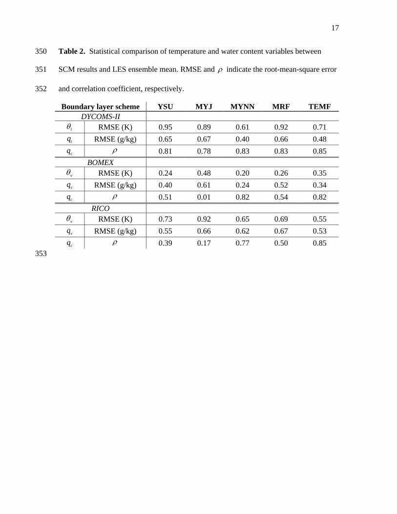
Table 2. Statistical comparison of temperature and water content variables between 350

SCM results and LES ensemble mean. RMSE and ρ indicate the root-mean-square error 351

and correlation coefficient, respectively. 352

Boundary layer scheme YSU MYJ MYNN MRF TEMF DYCOMS-II

lθ RMSE (K) 0.95 0.89 0.61 0.92 0.71

tq RMSE (g/kg) 0.65 0.67 0.40 0.66 0.48

cq ρ 0.81 0.78 0.83 0.83 0.85 BOMEX

vθ RMSE (K) 0.24 0.48 0.20 0.26 0.35

vq RMSE (g/kg) 0.40 0.61 0.24 0.52 0.34

cq ρ 0.51 0.01 0.82 0.54 0.82 RICO

vθ RMSE (K) 0.73 0.92 0.65 0.69 0.55

vq RMSE (g/kg) 0.55 0.66 0.62 0.67 0.53

cq ρ 0.39 0.17 0.77 0.50 0.85 353

18

354

355

Figure 1. Locations of the selected experiments in this study: the DYCOMS-II (D), the 356

BOMEX (B), and the RICO (R). The color map represents the averaged sea surface 357

temperature of remotely sensed data collected by the AVHRR during July, 2001.358

19

359

360

Figure 2. Vertical profile of a) liquid water potential temperature, b) total water vapor 361

mixing ratio, and c) cloud liquid water (in log-scale) for the DYCOMS-II experiments. 362

See text for more details.363

20

364

365

Figure 3. Vertical profile of a) potential temperature, b) water vapor mixing ratio, and c) 366

cloud liquid water (in log-scale) for the BOMEX experiments.367

21

368

369

Figure 4. Vertical profile of a) potential temperature, b) water vapor mixing ratio, and c) 370

cloud liquid water (in log-scale) for the RICO experiments. 371