
Evaluation of the TxDOT Texas Cone Penetration Test and ... · Evaluation of the TxDOT Texas Cone...
168
Evaluation of the TxDOT Texas Cone Penetration Test and Foundation Design Method Including Correction Factors, Allowable Total Capacity, and Resistance Factors at Serviceability Limit State by Rozbeh B. Moghaddam, BSCE, P.E., M.B.A. A Dissertation In Civil Engineering Submitted to the Graduate Faculty of Texas Tech University in Partial Fulfillment of the Requirements for the Degree of DOCTOR OF PHILOSOPHY Approved by William D. Lawson, P.E., Ph.D. Co-chair of the Committee Priyantha W. Jayawickrama, Ph.D. Co-Chair of the Committee Hoyoung Seo, Ph.D., P.E. Committee Member James G. Surles, Ph.D. Committee Member Mark Sheridan Dean of the Graduate School August 2016
Transcript of Evaluation of the TxDOT Texas Cone Penetration Test and ... · Evaluation of the TxDOT Texas Cone...

Evaluation of the TxDOT Texas Cone Penetration Test and Foundation Design
Method Including Correction Factors, Allowable Total Capacity, and Resistance
Factors at Serviceability Limit State
by
Rozbeh B. Moghaddam, BSCE, P.E., M.B.A.
A Dissertation
In
Civil Engineering
Submitted to the Graduate Faculty
of Texas Tech University in
Partial Fulfillment of
the Requirements for
the Degree of
DOCTOR OF PHILOSOPHY
Approved by
William D. Lawson, P.E., Ph.D.
Co-chair of the Committee
Priyantha W. Jayawickrama, Ph.D.
Co-Chair of the Committee
Hoyoung Seo, Ph.D., P.E.
Committee Member
James G. Surles, Ph.D.
Committee Member
Mark Sheridan
Dean of the Graduate School
August 2016

Copyright 2016, Rozbeh B. Moghaddam

Texas Tech University, Rozbeh B. Moghaddam August 2016
ii
ACKNOWLEDGEMENTS
I would like to thank my family: Akram, Mehdi, Hamzeh and Paola, Yeganeh and
Pouria, and Yekta, for their invaluable support throughout all these years.
I would like to express my deepest appreciation to my research committee members Dr.
Lawson, Dr. Jay, Dr. Seo, and Dr. Surles for their expert advice, guidance, and
understanding during my graduate studies and during the development of this
dissertation. I am grateful for their encouragement to pursue independent thinking.
I sincerely thank the Texas Department of Transportation for sponsoring the TCP
Reliability research study and Terracon, PSI, Rick Coffman (University of Arkansas),
The Arkansas State Highway and Transportation Department, the Missouri Department
of Transportation, the Louisiana Department of Transportation and Development, and
the New Mexico Department of Transportation in their assistance in providing data for
this study.
Last but not least, special thanks to all my friends in Texas, United States, and around
the World for their support during my studies.

Texas Tech University, Rozbeh B. Moghaddam, August 2016
iii
TABLE OF CONTENTS
ACKNOWLEDGMENTS……………………………………………………………………………………………….. ii
ABSTRACT ....................................................................................................................... viii
LIST OF TABLES .................................................................................................................. x
LIST OF FIGURES ............................................................................................................... xi
NOTATIONS ..................................................................................................................... xiii
CHAPTER I: INTRODUCTION .............................................................................................. 1
TCP FIELD TEST ............................................................................................................ 6
TCP FOUNDATION DESIGN CHARTS .............................................................................. 7
ORGANIZATION OF THE DISSERTATION ......................................................................... 8
CHAPTER II: HAMMER EFFICIENCY AND CORRECTION FACTORS FOR THE TXDOT
TEXAS CONE PENETRATION TEST ................................................................................... 11
ABSTRACT ..................................................................................................................... 11
INTRODUCTION ............................................................................................................. 12
THE TXDOT TEXAS CONE PENETRATION TEST ........................................................ 13
Description of the TCP test ....................................................................................... 13
History and development of the TCP test ................................................................. 14
COMPARISON OF SPT VS. TCP TESTS ......................................................................... 18
Correlation of blowcount results ............................................................................... 20
DEVELOPMENT OF CORRECTION FACTORS FOR SPT ................................................. 21
Standardization of the SPT blowcount ..................................................................... 21

Texas Tech University, Rozbeh B. Moghaddam, August 2016
iv
Early work by Fletcher and others ............................................................................ 22
Effect of Drilling Rod and Type of Sampler ............................................................ 23
Effect of Driving Technique and Hammer Type ...................................................... 24
Effect of Borehole Diameter ..................................................................................... 26
Development of correction factors for SPT N-values ............................................... 27
The overburden pressure correction for SPT ............................................................ 28
Contemporary practice for correcting SPT blowcount data ..................................... 30
Liquefaction studies .................................................................................................. 32
CORRECTIONS TO TCP BLOWCOUNT .......................................................................... 33
Need for TCP correction factors ............................................................................... 33
TxDOT policy ........................................................................................................... 33
RESEARCH DESIGN AND METHOD ............................................................................... 34
The TCP Reliability research study .......................................................................... 34
Field work and TCP blowcount data sources ........................................................... 34
Hammer energy readings .......................................................................................... 35
The TCP blowcount dataset ...................................................................................... 36
RESULTS FROM TCP BLOWCOUNT DATA ................................................................... 37
Hammer Efficiency for the TCP test (Er-TCP) ............................................................ 38
Development of Rod Length Correction Factors (CR-TCP) ........................................ 39

Texas Tech University, Rozbeh B. Moghaddam, August 2016
v
Side by side comparison of TCP and SPT Rod Length correction factors ............... 43
Development of Overburden pressure Correction Factors (CN-TCP) ......................... 44
Overburden correction factor CN-TCP ........................................................................ 49
OTHER FACTORS THAT MAY INFLUENCE TCP TEST HAMMER EFFICIENCY ............... 51
SUMMARY AND CONCLUSIONS ..................................................................................... 52
CHAPTER III: EVALUATION OF PREDICTED VALIDITY OF THE TEXAS CONE PENETRATION
DESIGN CHARTS FOR DEEP FOUNDATIONS BASED ON FULL SCALE LOAD TESTS ......... 54
ABSTRACT ..................................................................................................................... 54
INTRODUCTION ............................................................................................................. 55
THE TXDOT TEXAS CONE PENETRATION TEST ........................................................ 57
Description of the TCP test ....................................................................................... 57
TCP Design Charts ................................................................................................... 58
TCP Design Method for Deep Foundations.............................................................. 62
RESEARCH DESIGN AND METHOD ............................................................................... 63
Development of the Dataset .......................................................................................... 63
Allowable Predicted Total Capacity ............................................................................. 65
Allowable Measured Total Capacities .......................................................................... 67
DATA ANALYSIS............................................................................................................ 72
Qualitative Evaluation .............................................................................................. 75
Statistical Analysis .................................................................................................... 80
RESULTS ....................................................................................................................... 81

Texas Tech University, Rozbeh B. Moghaddam, August 2016
vi
Regression Models .................................................................................................... 82
Side-by-Side Comparison of all Measured Capacity Models ................................... 84
Evaluation of TCP charts based on Shaft and Base resistance ................................. 88
SUMMARY AND CONCLUSIONS ..................................................................................... 89
CHAPTER IV: RESISTANCE FACTORS AT SERVICEABILITY LIMIT STATE FOR LRFD OF
DEEP FOUNDATIONS USING THE TEXAS CONE PENETRATION TEST .............................. 93
ABSTRACT ..................................................................................................................... 93
INTRODUCTION ............................................................................................................. 94
TEXAS CONE PENETRATION (TCP) TEST .................................................................... 96
Description of TCP test ............................................................................................. 96
Application and use of TCP blowcount data for foundation design .......................... 97
LOAD AND RESISTANCE FACTOR DESIGN (LRFD) ..................................................... 99
Design approaches and methods................................................................................ 99
Ultimate Limit State (ULS) ....................................................................................... 99
Serviceability Limit State (SLS) .............................................................................. 100
LRFD of Deep Foundations .................................................................................... 101
SERVICEABILITY LIMIT STATE ANALYSIS ................................................................. 103
SLS Performance function ....................................................................................... 103
Tolerable Displacement ........................................................................................... 105
DEVELOPMENT OF SLS RESISTANCE FACTORS ........................................................ 108
Displacement Approach .......................................................................................... 108
Load Approach ........................................................................................................ 110
Calibration of Resistance Factors ............................................................................ 111
Texas Tech University, Rozbeh B. Moghaddam, August 2016
vii
RESEARCH DESIGN AND METHOD ............................................................................. 112
Dataset Development ............................................................................................... 112
Load Tests and TCP Borings ................................................................................... 113
Final Compiled Dataset ........................................................................................... 114
Load Corresponding to Tolerable Displacement and Design Load ........................ 114
Tolerable Displacement for the TCP design method ............................................... 117
RESULTS OF ANALYSES .............................................................................................. 119
Bias .......................................................................................................................... 120
Resistance Factors at SLS condition ....................................................................... 123
CONCLUSIONS ............................................................................................................. 128
Summary of Findings .............................................................................................. 128
Limitations/Further Study ............................................................................................... 129
CHAPTER V: SUMMARY AND CONCLUSIONS ................................................................. 131
REFERENCES ................................................................................................................... 140

Texas Tech University, Rozbeh B. Moghaddam August 2016
viii
ABSTRACT
This dissertation explores three different aspects of the Texas Department of
Transportation’s Texas Cone Penetration (TCP) test and its associated foundation
design charts. The first aspect has to do with the reliability of TCP data. The TCP test
hammer efficiency, rod length influence on the hammer efficiency, and effect of
overburden pressure on the TCP test blowcounts (NTCP) are explored. Results are
compared with published correction factors for the Standard Penetration Test (SPT).
The final dataset analyzed for the study, consisted of 293 TCP tests from which 135
tests were instrumented. Analyses showed a statistically significant relationship
between the TCP hammer efficiency and the rod length below ground surface. Rod
length correction factors (CR-TCP) and overburden correction factors (CN-TCP) were
obtained factors for the TCP test.
The second topic involves a quantitative and a qualitative evaluation of the predictive
validity of the Texas Cone Penetration (TCP) foundation design charts where allowable
measured total capacities determined from results of full-scale load tests were compared
to allowable predicted total capacities determined from TCP foundation design charts.
The final dataset analyzed compiled for this study consisted of 60 full scale load testes
comprising 33 driven piles and 27 drilled shafts. Allowable measured capacities were
determined using strength-based and serviceability-based models. Results from
analyses suggested that it is apparent that different performance assessment criteria
leads to different conclusions regarding the predictive validity of the TxDOT TCP

Texas Tech University, Rozbeh B. Moghaddam August 2016
ix
method for deep foundation design. The allowable predicted total capacity determined
from the TCP foundation design charts could be considered to be reasonable based on
a strength-based model, moderately over-conservative, to over-conservative according
to serviceability-based models. Further, it was observed that as the level of tolerable
settlement is increased, the interpretation of the TCP foundation design charts becomes
even more conservative.
The third topic identifies resistance factors for the serviceability limit state (SLS)
condition used in the load and resistance factor design (LRFD) of deep foundations
using the results from the TCP test. The performance function was established based on
load corresponding to tolerable displacement and design load. The compiled dataset
consisted of a total of 60 full scale load test cases comprising 33 driven piles and 27
drilled shafts. The loads corresponding to tolerable displacements were determined
using the load-settlement curves, and these loads were compared with the design load
determined using the TCP test method. Resistance factors for SLS conditions were
obtained for tolerable displacements using both the Monte Carlo simulation (MCS) and
the first order second moment (FOSM) calibration approaches.

Texas Tech University, Rozbeh B. Moghaddam, August 2016
x
LIST OF TABLES
2.1. Correlations between NSPT and NTCP………………………………………………………………........
21
2.2. Summary of existing Overburden correction factors (CN)……………………………….......
30
2.3. Field Research Sites and related TCP-Borings ………………………………………………..…..
35
2.4. Rod Length Correction Factors (CR) for TCP and SPT ……………………….........................
44
3.1. Compiled Dataset for Driven Piles in Soils …………………………………………………….......
74
3.2. Compiled Dataset for Drilled Shafts in Soils …………………………………………………….…
75
3.3. Regression line equation with p-value and R2, Driven Piles …………….............................
85
3.4. Regression line equation with p-value and R2, Drilled Shafts ………….............................
85
4.1. Compiled Dataset for Driven Piles ……………………………………………………………………...
116
4.2. Compiled Dataset for Drilled Shafts …………………………………………………………………….
117
4.3. Summary Statistics of Biases for Driven Piles and Drilled Shafts ………………………
122
4.4. Resistance Factors at Serviceability Limit State (SLS) for Foundations in Soils..
126

Texas Tech University, Rozbeh B. Moghaddam, August 2016
xi
LIST OF FIGURES
FIGURE CAPTIONS- CHAPTER II
2.1. TCP Test Conical Driving Point and Field Application………………………………… 14
2.2 (a) Allowable Shaft Resistance and (b) Base Resistance vs. TCP blows/12 inches
(TxDOT, 2012)……………………………………………………………………………………….
16
2.3. (a) Allowable Shaft Resistance (b) Allowable Base Resistance vs. TCP
Penetration/100 blows (TxDOT, 2012) )………………………………………………………..
16
2.4. Different Type of Hammers (a) Donut Hammer (b) Safety Hammer (c) Automatic
Hammer (Coduto et al. 2011 used with permission)……………………..................................
25
2.5. Standard Practice of NSPT Correction among State DOTs…………………………….... 31
2.6. Compiled dataset (a) TCP Blowcount Values NTCP (b) Average Hammer
Efficiency……………………………………………………………………………………………....
37
2.7. Scatterplot of Average Efficiency vs Rod length for all Soils………….......................... 42
2.8. N60-TCP and Effective Vertical Stress relationship for each TCP boring……………… 46
2.9. Scatterplot for Normalized TCP Blowcounts (NN-TCP) vs. Normalized Effective
Vertical Stress (’N)………………………………………………………………………………….
48
2.10. Effective Vertical Stress (’v) versus CN for TCP and SPT…………………………… 50
FIGURE CAPTIONS- CHAPTER III
3.1. TCP Test Conical Driving Point (TxDOT, 1999)………………....................................... 59
3.2. Design charts representing (a) allowable unit shaft resistance and (b) allowable
unit base resistance vs. TCP blows/30-cm (12-in), (TxDOT, 2012)………………………..
61
3.3. Illustrative example of determining 𝑃𝑎𝑃 for Case No. 23 of drilled
shafts………………………………………………………………………………………….................
66

Texas Tech University, Rozbeh B. Moghaddam, August 2016
xii
3.4. Case No. 23, Davisson’s ultimate Capacity Criterion and Serviceability
Criteria………………………………………………………………………………………………...
72
3.5. The relationship between 𝑃𝑎𝑀 and 𝑃𝑎
𝑃 compared to an equal prediction
line………………………………………………………………………………………………………
78
3.6. Scatterplot and fitted model, Driven Piles………………………………………………… 82
3.7. Scatterplot and fitted model, Drilled Shafts………………………..................................... 84
3.8. Side-by-Side Comparison of all Models analyzed, Driven Piles…................................ 86
3.9. Side-by-Side Comparison of all Models analyzed, Drilled Shafts………………….… 88
FIGURE CAPTIONS- CHAPTER IV
4.1. TCP test conical driving point (From TxDOT, 1999)………………................................ 97
4.2. TCP Foundation Design charts representing (a) allowable unit shaft resistance
and (b) allowable unit base resistance vs. TCP blows/30-cm (12-in), (TxDOT,
2012)……………………………………………………………………................................................
98
4.3. TCP Foundation Design charts representing (a) allowable unit shaft resistance
and (b) allowable unit base resistance vs. TCP penetration/100 blows (TxDOT, 2012) ……………………………………………………………………………...............................................
98
4.4. Loads corresponding to tolerable displacement (Qtol) and displacement from
design loads (Qd)……………………………………………………………………………………..
104
4.5. Tolerable displacement histograms for (a) driven piles and (b) drilled
shafts…………………………………………………………………………………...........................
119
4.6. Histograms and probability plots for driven piles (a and b, respectively) and for
drilled shafts (c and d, respectively)………………………….......................................................
122

Texas Tech University, Rozbeh B. Moghaddam, August 2016
xiii
NOTATIONS
The following symbols are used in this Dissertation
a and b Skempton (1986) soil dependent parameters
1 Slope for a linear model equation
o Intercept for a linear model equation
Cb Borehole diameter correction factor for SPT
CI Confidence Intervals
CN Overburden correction factor for SPT
CN-TCP Overburden correction factor for TCP
COV Coefficient of Variation
Cr Rod length correction factor for SPT
CR-TCP Rod length correction factor for TCP
Cs Sampler type correction factor for SPT
D Depth
DBASELINE Depth at which the fitted model has flattened
DR Relative Density
Em Measured hammer energy
Er Hammer Efficiency-SPT
Er-TCP Hammer Efficiency-TCP
Et Theoretical hammer energy
N1-60 SPT Blowcount standardized to 60% energy and corrected for overburden
N1-60-TCP TCP Blowcount standardized to 60% energy and corrected for overburden
N60 SPT Blowcount standardized to 60% energy
N60-TCP TCP Blowcount standardized to 60% energy
NN-TCP
Normalized TCP blowcount to a blowcount corresponding to a reference
stress
NSPT SPT Blowcount
NTCP TCP Blowcount
PI Prediction Intervals
'N Normalized effective vertical stress to a reference stress
SPT Standard Penetration Test
ref Reference Stress (i.e. 100 kPa, 2000 psf)
'v Effective vertical stress
TCP Texas Cone Penetrometer

Texas Tech University, Rozbeh B. Moghaddam, August 2016
xiv
g Performance Function
gSLS Serviceability Limit State Performance Function
L Span Length
Nsim Number of Simulations
Pf Probability of Failure
Q Load
Qd Design Load
Qd,TCP Predicted Capacity based on TCP design charts
QDL Dead Load
Qtol Load corresponding to the tolerable displacement
Qi Applied Load
QLL Live Load
Qt Total capacity
R Resistance
RM Measured Resistance
RP Predicted Resistance
SLS Resistance Factor at Serviceability Limit State
d Displacement under Design Load
Angular Distortion
Differential Settlement
t Resistance Factor for total resistance
d Resistance factor for design loads "Greater than 1.0"
trial Initial Resistance Factor for the Monte Carlo Simulation
tol Tolerable displacement
Bias
R-SLS Bias for Resistance at Serviceability Limit State
R Bias for Resistance
LL Bias for Live Load
DL Bias for Dead Load
Load Factor
Reliability Index

Texas Tech University, Rozbeh B. Moghaddam, August 2016
1
CHAPTER I
INTRODUCTION
This dissertation presents results of analyses completed for the evaluation of the Texas
Department of Transportation’s (TxDOT) Texas Cone Penetration (TCP) field test and its
associated foundation design method. The TCP field test is studied and correction factors
for the penetration index (NTCP) are developed. Furthermore, the predictive validity of TCP
foundation design charts have been evaluated by comparing the allowable measured
capacity (interpreted from full-scale load tests completed on deep foundations to allowable
predicted capacity (calculated from current published TCP foundation design charts).
Finally, considering the transition from allowable stress design (ASD) method to the Load
and Resistance Factor Design (LRFD) methodology, and the importance of the
serviceability of a structure, resistance factors at serviceability limit state for the TCP
foundation design method have been developed. All three contexts evaluated in this
dissertation share the common core of the TCP test and its foundation design charts with
different focal point. However, the collective outcome resulted from the detail exploration
of each topic will help to improve the TCP-based design of deep foundations.
As would be expected with its Texas roots, the TCP test has seen extensive application
throughout Texas to evaluate subsurface materials ranging from very soft clays, to shales
and fractured limestones, to hard rock. However, the use of TCP test and its associated
design charts are not limited to Texas practice only. Because of its applicability to a wide
range of geomaterials, the TCP test has been used not only throughout the United States
but also for international projects. According to FHWA (2016) Texas currently maintains

Texas Tech University, Rozbeh B. Moghaddam, August 2016
2
over 53,000 bridges in the National Bridge Inventory, and most of these bridges plus other
transportation infrastructure in Texas are supported by foundations designed in accordance
with the TCP method. Also, since Oklahoma DOT adopted the TCP test in the 1970s, the
TCP method has been used for the design of the foundations for most of the 23,000 bridges
in Oklahoma’s inventory. Collectively this indicates that over 12% of the nation’s bridges
are associated with the TCP test. Recently, a comprehensive research program in Missouri
evaluated a modified version of the TCP test for bridge foundation design applications
using LRFD concepts (Loehr et al. 2011). The TCP test was introduced to an international
audience during a workshop sponsored by the Port and Airport Research Institute of Japan,
and the application of the method for the design of deep foundations was discussed as part
of Advance in Deep Foundations in Japan, (Vipulanandan, C. 2007). Furthermore, the TCP
test has been used in Korea for field explorations associated with a bridge abutment
overlying intermediate geomaterials and soft rock where cores would have been recovered
in fragments because of joint structures (Nam et al. 2013). In light of the preceding, the
scope of the TCP test and its associated foundation design charts is significant well beyond
its regional origins. Therefore, the presence of the TCP test and its associated foundation
design method in the deep foundations expert community is noteworthy.
Technological advancements have certainly impacted most engineering disciplines
including the geotechnical engineering field. Tools and methods used in the geotechnical
field exploration have been modified and improved throughout the United States. One of
the notorious changes is the introduction and implementation of automatic hammers which
has substituted traditional hammers used in the past during geotechnical drilling and

Texas Tech University, Rozbeh B. Moghaddam, August 2016
3
sampling operations. Aside from drilling and sampling, many times, if not at all times, a
penetration index is recorded while performing a dynamic field testing. Throughout many
years, these penetration indices have been correlated to soil strength parameters, and
further, these correlations have been used for the design of many geotechnical elements
including deep foundations.
The TCP test and its associated foundation design charts, are the great example related to
the above stated situation in geotechnical engineering. The TCP method dates back to
1940s when the use of hammers other than an automatic hammer was common. Penetration
indices were correlated to soil strength for the development of TCP foundation design
charts. In current practice, automatic hammers are used to determine penetration indices
but TCP design charts were developed based on a non-automatic hammers and are used for
the design of deep foundations. Therefore, the penetration indices recorded based on
automatic hammers are not the same as those recorded using a none-automatic hammer
which directly impacts the TCP-based design of deep foundation.
Aside from type of hammer, other factors such as type of soil in which the test is being
performed, the diameter of the borehole, existence of fluid in the borehole, among others
may influence the penetration indices and further impact the design parameters determined
from TCP foundation design charts.
Considering previous published work and research studies completed for other
geotechnical dynamic field tests to address similar issues as stated in the preceding

Texas Tech University, Rozbeh B. Moghaddam, August 2016
4
paragraphs, it is reasonable to consider the development of correction factors for the TCP
test to account for type of hammer and other influential factors. The first topic presented
in this dissertation explores factors influencing the TCP test blowcounts (NTCP) including
hammer efficiency, rod length, and overburden pressure. Correction factors for the NTCP,
will yield a more refined penetration index that can be used for the determination of
strength parameters from the TCP foundation design charts to further calculate the axial
capacity for a deep foundation element. For this part of the dissertation it was hypothesized
that: (1) There is a relationship between TCP Hammer Efficiency and the length of drilling
rod below ground surface, and (2) There is a relationship between NTCP and the overburden
pressure.
After developing correction factors for the NTCP, another variable that directly influences
the design of deep foundation using the TCP design method, is the predictive validity of
the TCP model itself. Therefore, it is reasonable to consider a detailed analysis and
evaluation of the existing TCP foundation design charts. Another topic thoroughly studied
in this dissertation was related to the evaluation of the predictive validity of the TCP
foundation design charts by comparing allowable measured total capacity to the allowable
predicted total capacity. In engineering design, the allowable load on a structural
component may be determined based on strength-based criteria or serviceability-based (i.e.
settlement-based) criteria. Within the context of deep foundations, the strength-based
allowable load capacity can be defined as ultimate capacity divided by an appropriate factor
of safety. The serviceability-based approach consisted of loads corresponding to vertical
displacements determined from load-settlement curves. In geotechnical engineering,

Texas Tech University, Rozbeh B. Moghaddam, August 2016
5
deformations presented at the head of the deep foundation are translated to vertical
settlements noted in the superstructure. When settlements are larger than an established
tolerable settlement, then it is considered that the foundation element has reached a
serviceability limit condition, and the performance of the superstructure is not satisfactory.
For this part of the dissertation it was hypothesized that the predictive validity of the TCP
foundation design charts is within higher confidence that the allowable measured capacity
is equal or greater than the allowable predicted capacity for serviceability-based model
compared to a strength-based model.
Once the TCP field test and foundation design method were evaluated, the application of
this method can be analyzed. In geotechnical engineering and more specifically in the case
of deep foundation design, deformations can be translated to vertical displacement of the
foundation element which causes settlement in the superstructure. Most structures and in
particular, transportation structures such as bridges, suspend service operations as soon as
one of the structure’s members experiences displacements beyond a tolerable
displacement. This could well explain that geotechnical designs are mainly displacement-
based designs rather than strength-based designs. Although, most of geotechnical design
are performed following a strength-based model, the performance of the foundation or the
superstructure is settlement dependent.
Considering that (1) geotechnical engineers working on projects funded by the Federal
Highway Administration (FHWA) have been transitioning from the ASD approach to the
LRFD methodology, (2) the TCP-based designs are mainly used for transportation

Texas Tech University, Rozbeh B. Moghaddam, August 2016
6
infrastructures funded by FHWA, and (3) the geotechnical designs are mainly settlement
or serviceability governed designs, then it is an equitable interest to analyze the TCP test
based on the LRFD requirements focused on the serviceability instead of strength. In this
topic, resistance factors at serviceability limit state were developed for the LRFD of deep
foundations using the TCP foundation design charts. For this context it was hypothesized
that as the foundation element is allowed to experience higher settlements, higher
resistance factors at serviceability limit state is determined.
TCP FIELD TEST
The TCP test is a dynamic field penetration test which assesses the consistency of the
material encountered during geotechnical exploration. This test method is documented as
TxDOT Designation Tex-132-E, “Test Procedure for Texas Cone Penetration” (TxDOT
1999). The TCP test uses a 77.0-kg (170-lb) hammer with 60-cm (24-in) drop to force a
7.6-cm (3-in) diameter steel cone into the soil or rock formation. In current practice, the
penetration is to be achieved in three separate increments. The first increment is completed
to ensure proper seating, which consists of driving the cone 12 blows or approximately 15-
cm (6-in), whichever happens first. The TCP blowcount is then determined as the sum of
the number of blows required to achieve second and third 15-cm (6-in) increments of cone
penetration. The total blowcount or NTCP corresponding to 30-cm (12-in) penetration is
used to obtain design parameters. In very hard materials such as rock and intermediate
geomaterials (IGM), after the proper seating process is completed, the cone is driven 100
blows and the penetration value for the first and second 50 blows are recorded.

Texas Tech University, Rozbeh B. Moghaddam, August 2016
7
TCP FOUNDATION DESIGN CHARTS
The 1956 edition of the Foundation Exploration and Design Manual provides a series of
correlation curves illustrating unit shear strength estimation based on NTCP. These
correlation curves were based on relationships established between TCP test data and
laboratory-measured shear strength. To obtain soil strength parameters for this purpose,
undisturbed samples were collected and tested using the triaxial test procedure (THD
1956). Based on data obtained from field and laboratory studies, correlation charts were
developed and published in two separate sets of design charts. The first set was developed
for soils with TCP blowcounts less than 100 per 30-cm (12-in); whereas, the second set is
for geomaterials with blowcounts greater than 100 blows per 30-cm (12-in) (i.e. penetration
per 100 blows). The current design charts reflect the allowable stress design philosophy
and present allowable strength values corresponding to a Factor of Safety (FS) of 2.0.
Different literature may refer to the foundation shaft resistance and base resistance using
other terminologies such as skin resistance and toe bearing or skin friction and point
bearing. The TxDOT’s Geotechnical Manual refers to these resistances as allowable skin
friction and allowable point bearing. Furthermore, design charts are categorized based on
soil classification where capacity models for fat clay (CH), Lean Clay (CL), Clayey Sand
(SC), and OTHER soils have been developed. According to the design procedure TxDOT
(2012) any soil calssified as SP, SW, SM, and ML is considered as OTHER category.

Texas Tech University, Rozbeh B. Moghaddam, August 2016
8
ORGANIZATION OF THE DISSERTATION
The work completed for a critical evaluation of the TCP field test and its associated
foundation design charts including the development of TCP test blowcount correction
factors, assessment of current TCP foundation design charts based on full-scale load test
results, and the development of resistance factors at the serviceability limit state (SLS) used
in the Load and Resistance Factor Design (LRFD) of Deep Foundations are documented
in this dissertation and presented as follows:
Chapter 1 presents a brief description of the topics explored and developed throughout the
dissertation. The TCP test and its regional, national, and international presence is briefly
discussed followed by a summary of the rationale behind the need for corrections to the
TCP penetration index. Furthermore, a synthesized description of the evaluation of the TCP
foundation design charts based on a comparisons between allowable measured capacities
determined from results of full-scale load tests and allowable predicted capacities
determined using the TCP foundation design charts is presented. Finally, the importance
of settlement governed design of deep foundations and the development of resistance
factors at serviceability limit state for the LRFD of deep foundations using the TCP method
is explained.
Hammer efficiency data, rod length influence on the hammer efficiency, and overburden
pressure correction factors for the Texas Cone Penetration (TCP) test blowcounts (NTCP)
are explored in Chapter 2. Results of analyses are compared to published correction factors
developed for the Standard Penetration Test (SPT). The effort associated with data

Texas Tech University, Rozbeh B. Moghaddam, August 2016
9
collection and statistical analyses are described in detail. At the end of the chapter, results
for hammer efficiency, rod length correction factors, and overburden correction factors are
presented.
In chapter 3, presents a detailed evaluation of the TxDOT’s TCP foundation design charts
by comparing the allowable predicted total capacity determined using the TCP foundation
design charts to the allowable measured total capacity obtained from full scale load tests
completed for driven piles and drilled shafts in soils. Two different approaches were used
to determine the allowable measured total capacity from results of full-scale load test: (1)
strength-based method, and (2) serviceability-based approach. After determining the
allowable measured total capacity and the allowable predicted total capacity, these data
were analyzed based on (1) a qualitative evaluation where all data were plotted and
compared to an equal prediction line, and (2) a quantitative evaluation where statistical
analysis and linear regression models were developed to analyze the relationship between
allowable measured total capacity and the allowable predicted total capacity.
Chapter 4 presents the calibration process and the development of resistance factors for the
serviceability limit state (SLS) condition used in the load and resistance factor design
(LRFD) of deep foundations using the results from Texas Cone Penetration (TCP).
Determination of statistical parameters such as mean and coefficient of variation for the
bias is described and resistance factors for SLS conditions were obtained using both the
Monte Carlo simulation (MCS) and the first order second moment (FOSM) calibration
approaches.

Texas Tech University, Rozbeh B. Moghaddam, August 2016
10
Chapter 5 presents a summary of the analyses and results obtained for all topics explored
in this dissertation, discusses notable findings, and highlights key contributions. Research
studies and future work recommended for the enhancement of results presented in this
dissertation are presented in this chapter. Furthermore, limitations of compiled datasets for
each topic discussed and analyzed in this dissertation are noted. Finally, based on the
findings of this dissertation, a detailed discussion of the TxDOT TCP test, its foundation
design charts, and the applicability of this method is presented where important conclusions
are highlighted.

Texas Tech University, Rozbeh B. Moghaddam, August 2016
Note 1: Moghaddam R.B., Lawson, W.D., Surles, J.G., Seo H., Jayawickrama, P.W. (2016), “Hammer
Efficiency and Correction Factors for the TxDOT Texas Cone Penetration Test”, Journal of Geotechnical
and Geoenvironmental Engineering, Submitted June, 7th, 2016
11
CHAPTER II
HAMMER EFFICIENCY AND CORRECTION FACTORS FOR THE TXDOT TEXAS
CONE PENETRATION TEST 1
ABSTRACT
This study analyzes blowcount fata from instrumented Texas Cone Penetration (TCP) tests.
TCP hammer efficiency, rod length influence on the hammer efficiency, and overburden
pressure correction factors for the TCP blowcounts (NTCP) are explored. Results are
compared to published correction factors for the Standard Penetration Test (SPT). The final
dataset analyzed for this study consisted of 293 TCP tests from which 135 tests were
instrumented. TCP hammer efficiency values for automatic CME hammers ranged from
74% to 101% with an average of 89%. Analyses showed a statistically-significant
relationship between the TCP hammer efficiency and the rod length below ground surface.
Statistical models were developed for undifferentiated soils and rod length correction factor
for the TCP test (CR-TCP) were obtained ranging from 0.90 to 1.00. In a second analysis the
relationship between the overburden pressure and the NTCP was explored and a
mathematical expression for the overburden correction factors for the TCP blowcount
value (CN-TCP) was determined. This work is the first study that has been completed where
corrections to NTCP are explored and the outcome benefits the geotechnical engineering
community using the TCP test and foundation design method.

Texas Tech University, Rozbeh B. Moghaddam, August 2016
12
INTRODUCTION
This paper presents correction factors for blowcount values (NTCP) from the Texas Cone
Penetration (TCP) test, a dynamic field penetration test which is similar to yet different
from the Standard Penetration Test (SPT). For over 60 years, the TCP test and its associated
foundation design charts have been used successfully for the design of drilled shaft and
driven pile foundations that support tens of thousands of bridges and other major
transportation infrastructure throughout Texas and parts of Oklahoma. Data for this study
were obtained as part of a program of 293 TCP tests obtained from 21 geotechnical borings
in five states. These data were used to identify the average hammer efficiency for the TCP
test using an automatic hammer, and also to develop rod length correction factors and
overburden pressure correction factors for the NTCP values.
The main purpose of correction factors for field penetration blowcount values is to achieve
consistent and reliable input data for the foundation design procedures associated with the
tests. In the case of SPT, several studies have been completed to address the impact of
different factors on the hammer efficiency which further influences NSPT. In contrast to
SPT, no published work discusses a corrected NTCP nor addresses the influence of different
factors on TCP hammer efficiency. This paper contributes to the geotechnical engineering
community where the TCP design charts are used as the primary method for the design of
deep foundations. The factors presented in this paper help to standardize NTCP and further
obtain accurate design parameters for foundation design based on the TCP design charts.

Texas Tech University, Rozbeh B. Moghaddam, August 2016
13
The TCP test and its associated foundation design method are introduced and compared to
the SPT to further highlight similarities and differences. To set the stage for the analyses
presented in this paper, a review of the history of the TCP test and the development of
correction factors for the SPT are described. Tasks associated with the field data collection
for this study followed by statistical analyses and results are discussed in detail. Finally,
hammer efficiency for the TCP test and rod length correction factors for NTCP are
developed and compared to existing factors for the SPT. Furthermore, the effect of the
overburden pressure on the variation of NTCP is analyzed and discussed.
THE TXDOT TEXAS CONE PENETRATION TEST
Description of the TCP test
The TCP test is a dynamic field penetration test which assesses the consistency of the
material encountered during geotechnical exploration. This test method is documented as
TxDOT Designation Tex-132-E, “Test Procedure for Texas Cone Penetration” (TxDOT
1999). The TCP test uses a 77.0-kg (170-lb) hammer with 0.61-m (24-in) drop to force a
7.6-cm (3-in) diameter steel cone into the soil or rock formation, Figure 2.1.

Texas Tech University, Rozbeh B. Moghaddam, August 2016
14
(a) TCP Conical Driving Point
(TxDOT 1999)
(b) Field Application of the TCP Test
(TxDOT 1999)
Figure 2.1. TCP Test Conical Driving Point and Field Application
In current practice, penetration for the TCP test is performed in three separate increments.
The first is to achieve proper seating, consisting of driving the cone 12 blows or
approximately 15-cm (6-in), whichever comes first. The TCP blowcount is then
determined as the sum of the number of blows required to achieve the second and third
15-cm (6-in) increments. The total blowcount or NTCP corresponding to 30-cm (12-in)
penetration is used to obtain design parameters. In very hard materials such as rock and
intermediate geomaterials (IGM), after the proper seating process, the cone is driven 100
blows and the penetration value for the first and second 50 blows are recorded, with the
NTCP value reported as centimeters (inches) of penetration per 100 blows.
History and development of the TCP test
In the 1940s, the newly-formed Bridge Foundation Soils group of the Texas Highway
Department (THD) Bridge Division identified the need for developing a unified method

Texas Tech University, Rozbeh B. Moghaddam, August 2016
15
for the characterization of geomaterials and the design of deep foundations. The TCP test
method was developed by the Bridge Group as an in-situ test method for evaluating the
broad range of geologic materials encountered in foundation construction (TxDOT 2000).
The TCP-based foundation design method was introduced in the 1956 edition of the
Foundation Exploration and Design Manual (THD, 1956). This manual provided a series
of correlation relationships for foundation design which were established based on TCP
test blowcount data (NTCP) and laboratory-measured shear strength using the triaxial test
procedure (THD, 1956). The charts published in 1956 were refined in 1972, 2000, and
2012, and two sets of design charts now exists. The first set was developed for the
prediction of unit shaft resistance (i.e. skin friction) and unit base resistance (i.e. point
bearing) for soils with TCP blowcounts less than 100 blows/30-cm (blows/foot), Figure
2.2. The second set is for geomaterials with blowcounts greater than 100 blows/30-cm
(blows/foot) (i.e. penetration per 100 blows), Figure 2.3. The current design charts reflect
the allowable stress design philosophy and present allowable strength values.

Texas Tech University, Rozbeh B. Moghaddam, August 2016
16
(a) (b)
Figure 2.2 (a) Allowable Shaft Resistance and (b) Base Resistance vs. TCP blows/12
inches (TxDOT, 2012)
(a) (b)
Figure 2.3 (a) Allowable Shaft Resistance (b) Allowable Base Resistance vs. TCP
Penetration/100 blows (TxDOT, 2012)

Texas Tech University, Rozbeh B. Moghaddam, August 2016
17
The TCP test and its associated foundation design method have been used regionally,
nationally and internationally. As would be expected with its Texas roots, the TCP test
has seen extensive application throughout the state to evaluate subsurface materials
ranging from very soft coastal clays, to shales and weathered/fractured limestones, to hard
and brittle rock. Texas currently maintains over 53,000 bridges in the National Bridge
Inventory (FHWA 2016), and most of these bridges plus other transportation
infrastructure in Texas are supported by foundations designed in accordance with the TCP
method. The Oklahoma DOT adopted the TCP test and foundation design approach in the
1970s, so the foundations for most of the 23,000 bridges in Oklahoma’s inventory were
also designed using the TCP method. Collectively this means over 12% of the nation’s
bridges are associated with the TCP test. The TCP test is discussed in NCHRP Synthesis
360 (Turner 2016), and owing to competitive opportunities for Texas’ major
transportation infrastructure projects, geotechnical practitioners and academics
nationwide have had occasion to learn about and use the TCP test. More recently, a
comprehensive research program in Missouri evaluated a modified version of the TCP
test for bridge foundation design applications using LRFD concepts (Loehr et al. 2011).
The TCP test was introduced to an international audience of deep foundation engineers in
Japan (Vipulanandan, C. 2007), and the TCP test has been used in Korea for field
explorations associated with a bridge abutment overlying intermediate geomaterials and
soft rock where cores would have been recovered in fragments because of joint structures
(Nam et al. 2013). Collectively then, the scope of the TCP test is significant well beyond
its regional origins.

Texas Tech University, Rozbeh B. Moghaddam, August 2016
18
COMPARISON OF SPT VS. TCP TESTS
The SPT is an international standard for measuring soil penetration resistance and
obtaining a representative disturbed soil sample for identification purposes (ASTM 2016)
and has adopted a 63-kg (140-lb) hammer mass with a falling height of 76-cm (30-in) to
force a 45-cm (18-in) sampler (i.e. split spoon) with a coupler and driving shoe to penetrate
into soil strata. The conventional SPT driving procedure where blows are recorded for each
of three 15-cm (6-in) increments was introduced in 1954, and the SPT was adopted in 1958
as ASTM Standard D 1586, “Standard Test Method for Standard Penetration Test (SPT)
and Split Barrel Sampling of Soils”.
The form of the TCP test is similar to the SPT in that a steel driving point is advanced into
subsurface material at the bottom of a borehole by hammer strikes, with blowcounts
recorded in three 15-cm (6-in) increments. However, in certain aspects the TCP test differs
from the SPT. The TCP test does not use a split-barrel sampler but rather a solid steel
conical point, Figure 2.1. Hence, the TCP test cannot and does not collect a soil sample.
Also, because of its more robust solid steel design, TCP test refusal is defined as resistance
to penetration greater than 100 blows/30-cm (12-in), so the TCP test is suitable for
evaluating harder geomaterials and rock. In contrast, SPT refusal is customarily achieved
at resistance to penetration greater than 50blows/15-cm (6-in), or when there is no observed
advance of the sampler during the application of 10 successive blows.
Another difference between the SPT and the TCP test is the magnitude of their blowcount
values. The correlation between NTCP and NSPT is not linear, and NSPT values are typically
Texas Tech University, Rozbeh B. Moghaddam, August 2016
19
20% to 60% lower than NTCP values, other things being equal (Touma et al. 1972). It is
possible to gain an intuitive sense about this by comparing the hammer energy and the
sampler area for the two tests. The theoretical hammer energy for the tests is roughly
equivalent – 475 N-m (4,200 in-lbf) for the SPT vs. 461 N-m (4,080 in-lbf) for the TCP.
But the cross-sectional area of the samplers is quite different. The nominal cross-sectional
area for an unplugged SPT split spoon is 1,071 mm2 (1.66 in2) compared to the TCP conical
point with cross sectional area of 4,561 mm2 (7.07 in2). Thus, it ought to take a lot less
energy to drive an SPT split barrel sampler than the TCP cone, so SPT blowcounts should
be significantly lower than TCP blowcounts in the same material. This is in fact the case.
Since the 1970s, research has shown that blowcounts obtained from the SPT (NSPT) are
sensitive to factors such as hammer energy, rod length, type of soil, borehole diameter, and
others. In the case of SPT a significant body of literature and research exists to facilitate
direction and guidance for correcting NSPT values and further use a standardized NSPT for
design. In contrast, for the TCP test, published work has not been completed exploring the
effects of these same factors, and perhaps other factors influencing the resistance to
penetration.
It is important to mention that throughout this paper, detailed discussion and mathematical
expressions regarding the SPT and the TCP test are presented. For purposes of clarity and
consistency all factors, equations, and parameters associated with the TCP test will have
the subscript “TCP”. Any other geotechnical field testing parameter presented without the
subscript will be associated with the SPT.

Texas Tech University, Rozbeh B. Moghaddam, August 2016
20
Correlation of blowcount results
Another difference between the SPT and the TCP test is the magnitude of their blowcount
values, and it can be stated upfront that NSPT values are typically 20% to 60% lower than
NTCP values, other things being equal. It is possible to gain an intuitive sense about this by
comparing the hammer energy and the sampler area for the two tests. The theoretical
hammer energy for the tests is roughly equivalent – 475 N-m (4,200 in-lbf) for the SPT vs.
461 N-m (4,080 in-lbf) for the TCP. But the cross-sectional area of the samplers is quite
different. The nominal cross-sectional area for an unplugged SPT split spoon is 1,071 mm2
(1.66 in2) compared to the TCP conical point with cross sectional area of 4,561 mm2 (7.07
in2). Thus, it ought to take a lot less energy to drive an SPT split barrel sampler than the
TCP cone, so SPT blowcounts should be significantly lower than TCP blowcounts in the
same material. This is in fact the case.
Burmister (1948) presented an energy-area equation to correct NSPT when compared to
different but similar in-situ penetration tests. Lacroix and Horn (1973) presented a theory
where the resistance to penetration from a non-standard test is compared to a standardized
penetration test such as SPT. These resistances to penetration are correlated based on
parameters creating the driving energy.
TxDOT published correlations based on the research done by Touma and Reese (1972)
which was the first side-by-side correlation between SPT and TCP blowcount values. In
contrast to energy-area equations, the correlations presented by Touma and Reese (1972)

Texas Tech University, Rozbeh B. Moghaddam, August 2016
21
identify a distinction between coarse and fine grained soils. Building on this work, Lawson
et al. (2016) developed new correlation factors between NSPT and NTCP based on a larger
side-by-side dataset. Table 2.1 summarizes published correlations between NSPT and NTCP.
Table 2.1. Correlations between NSPT and NTCP
DEVELOPMENT OF CORRECTION FACTORS FOR SPT
Standardization of the SPT blowcount
To reduce the variability of NSPT due to multiple factors associated with the test, several
researchers have recommended the standardization of NSPT to a specific level where the
influence of these factors has been addressed through correction factors. Numerous
technical reports and research studies have been published addressing the factors that may
influence the NSPT including hammer type, sampler, driving mechanism, depth of test,
borehole diameter, and physical aspects of tools used during the test. See Palmer and Stuart
(1957), Fletcher (1965), Ireland (1970), DeMello (1971), Brown (1977), Schmertmann
Reference Type of
Correlation
Correlation Application
Burmister
(1948)
Energy Area NSPT = 0.23NTCP Open Split Spoon
All Soils
Lacroix and
Horn (1973)
Energy Area NSPT = 0.43NTCP Closed Split Spoon
All Soils
Touma and
Reese (1972)
Side-by-Side NSPT = 0.7NTCP
NSPT = 0.5NTCP
Fine Grained Soils
Coarse Grained Soils
Lawson et al.
(2016)
Side-by-Side logN60SPT = 0.1830 + 0.7463 log N60TCP
logN60SPT = 0.7436 + 0.303 log N60TCP
Fine Grained Soils
Coarse Grained Soils

Texas Tech University, Rozbeh B. Moghaddam, August 2016
22
(1979), Uto (1981), Kovacs and Salomone (1982), Seed (1984), Skempton (1986), Daniel
et al. (2005), Odebrecht et al. (2005), and Schnaid (2009). The work completed by these
researchers mainly focused on the determination of a standard NSPT where all the
variabilities associated with the test procedure are accounted for. In later years, this topic
continued to evolve with slightly different focus. Work done by Aggour (2001) and Idriss
and Boulanger (2004, 2012, and 2015) focused on the calibration of NSPT for purposes of
liquefaction and corrections for overburden pressure after the work presented by Skempton
(1986).
Early work by Fletcher and others
Between 1920s and 1930s the SPT was considered as a standard test by introducing the 63-
kg (140-lb) hammer, 76-cm (30-in) drop height, and 5-cm (2-in) outer diameter split
sampler. The influence of human factors and equipment associated with the execution of
the SPT were outlined and examined by Fletcher (1965). The application of the SPT in
both granular and cohesive soils was studied emphasizing limitations and problems
associated with the resistance to penetration including drop height and weight drop
(Fletcher, 1965).
DeMello (1971) presented the first comprehensive state of the art report on SPT where the
sampler penetration and factors impacting the penetration resistance were explored. These
factors were categorized as human factor, energy variation, borehole diameter, use of drill
mud, type of soil, and depth. The human factor was considered unsolvable other than

Texas Tech University, Rozbeh B. Moghaddam, August 2016
23
exercising due care or the implementation of statistical analyses where possible, to reduce
systematic errors (DeMello, 1971).
Effect of Drilling Rod and Type of Sampler
Palmer and Stuart (1957) approached the effect of drilling rod size on the energy traveled
through the drilling rod and analyzed this effect using the wave equation. The conclusion
was that the rod size had no major effect on the energy traveled except when the test is
performed in very soft soil.
The influence of the physical aspect of drilling rod on NSPT was evaluated by Brown (1977)
where results from six SPT borings using AWJ and NWJ rods were analyzed. The findings
of the study showed no significant difference between the NSPT obtained from the AWJ rod
and NWJ rod. Uto et al. (1981) compared results of SPT conducted using AWJ rod and JIS
(i.e. the NWJ version of the rod in Japan) in two different soil types. Results obtained from
the study indicated similar NSPT except that a slightly higher N-values were detected when
the test was conducted in hard clay.
Schmertmann (1978) and Schmertmann and Palacios (1979) evaluated the effect of the rod
size on the energy traveled by using strain gauges beneath the anvil and above the split
spoon sampler. The results indicated small variations of NSPT which were mainly related to
rod whip effect and varying slack of the thread joints.
Schmertmann and Palacios (1979) further explored the effect of type of sampler on the
SPT blowcount values, NSPT. The type of sampler refers to whether the split spoon is used

Texas Tech University, Rozbeh B. Moghaddam, August 2016
24
with or without a liner. The internal wall friction in the sampler is reduced when a liner is
not used resulting in larger sample recovery (Schmertmann and Palacios, 1979) but in
many cases when the SPT is completed without a liner the NSPT is affected due to plugging.
Effect of Driving Technique and Hammer Type
The donut hammer, safety hammer, and automatic hammer are three commonly-used
hammers in geotechnical exploration for field penetration tests such as the SPT and the
TCP, Figure 2.4. In a donut hammer a circular-shaped mass is lifted by the rope-cathead
arrangement and released by the driller to create the impact at the anvil level. In operations
where a safety hammer is used, the anvil is located inside a 63-kg (140-lb) sleeve (for SPT)
which is lifted and released similar to a donut hammer. In contrast, modern automatic
hammers use a mechanical apparatus to reliably achieve the required height and an
unrestrained hammer drop.

Texas Tech University, Rozbeh B. Moghaddam, August 2016
25
(a) (b) (c)
Figure 2.4. Different type of Hammers (a) Donut (b) Safety (c) Automated
(Coduto et al. 2011 used with permission)
A comparison study completed by Ireland et al. (1970) and further discussed by Frydman
(1970) showed that the NSPT obtained from a cat-head hoist was 1.4 times the NSPT obtained
from a self-tripping hammer. These results were confirmed by a further study (Lowther,
1973) indicating that the driving mechanism or release method has a significant impact on
the NSPT.
For a cat-head hoist mechanism (Kovacs et al. 1977) demonstrated that the impact velocity
could be affected by the number of turns of rope around the cat-head, the friction between
the rope and cat-head, and rope deterioration. In a more detailed study Kovacs and
Salomone (1982) completed 17 total field tests using safety hammers for eight tests and

Texas Tech University, Rozbeh B. Moghaddam, August 2016
26
donut hammer for the remaining nine tests. Energy ratio (i.e. hammer efficiency) of 50%
and 48% were reported for the safety and donut hammer, respectively.
For the SPT, Nixon (1982) examined the results from studies completed for the European
Standard to the results of studies completed in US and Japan. From the comparison, it was
concluded that before a final standardization of the SPT, it is important to conduct
comprehensive research studies to explore the influence of the type of hammer and sampler
on the NSPT. In another study (Robertson et al. 1983) alternated tests with a donut and safety
hammer. These tests were carried out in the same borehole utilizing the same drill rig and
drill rod with a slip-rope release method. The results from 16 tests showed an average of
62% energy ratio for the safety hammer and 43% for the donut hammer. This finding
followed the same pattern presented in the work completed by Kovacs and Salomone
(1982) where the safety hammer had higher energy ratio compared to the donut hammer.
Effect of Borehole Diameter
At the beginning of its origin, the SPT was completed at the bottom of 2.5-in or 4.0-in.
diameter boreholes. These borehole diameters are still considered common in geotechnical
engineering practice. For example in Japan, diameters such as 2.6-in and 3.4-in are used
(Yoshimi and Tokimatsu, 1983). However, in other places, boreholes with 6.0-in and 8.0-
inch diameters have been reported (Nixon, 1982). In cohesive soils the impact of borehole
diameter on NSPT can be neglected, however, in the case of sandy soils lower NSPT is
obtained with larger diameters (Lake, 1974 and Sanglerat & Sanglerat, 1982). This effect

Texas Tech University, Rozbeh B. Moghaddam, August 2016
27
is associated with the disturbance of the soil during testing and sampling procedure.
(Sanglerat and Sanglerat, 1982).
Development of correction factors for SPT N-values
The energy delivered into the drilling rod and the sampler is impacted by the release
method and type of hammer (Skempton, 1986). Based on the results of studies described
above and recommendations presented by Seed et al. (1984), a correction to the NSPT was
proposed by Skempton (1986) based on the hammer energy ratio reported in the United
States. The hammer energy ratio (Er), also termed “hammer efficiency”, refers to the
relationship between measured energy (Em) and theoretical energy (Et), Er = Em/Et *100%.
NSPT values with a known energy ratio can be normalized to 60% of hammer efficiency
using equation (2.1).
N60 = NSPT
Er
60 (2.1)
In equation (2.1), N60 is the normalized NSPT for 60% hammer efficiency, NSPT is the SPT
blowcount for 30-cm (12-in) penetration, and Er is the hammer efficiency for a specific
type of hammer.
In addition to the energy ratio, Skempton (1986) further developed work done by
Schmertmann and Palacios (1979) who determined that the required energy to drive the
sampler is increased as the rod length increases. He also considered research completed by
Texas Tech University, Rozbeh B. Moghaddam, August 2016
28
Seed et al. (1984) who showed that approximately 20% more blows corrected for 60% of
hammer efficiency were required to drive as SPT sampler without a liner. From this work,
Skempton (1986) determined correction factors for rod length, sampler type, and borehole
diameter, and modified Equation (2.1) by introducing correction factors:
N60 = NSPT Er
60CrCbCs (2.2)
In Equation (2.2), Cr, Cb, and Cs are correction factors to the SPT blowcounts to account
for hammer efficiency, rod length, borehole diameter, and type of sampler, respectively.
These correction have appeared in standard geotechnical textbooks such as Geotechnical
Engineering: Principles and Practice by Coduto et al. (2011) and Fundamentals of
Geotechnical Engineering by Das et al. (2014).
The overburden pressure correction for SPT
According to Meyerhof (1957) the penetration resistance increases linearly with depth, and
at a constant vertical stress, the resistance to penetration also increases at a rate
approximately equal to the relative density squared, Equation (2.3).
NSPT = 𝐷𝑅2 (a + b𝜎′
𝑣) (2.3)
In Equation (2.3) a and b are soil dependent factors, DR is the relative density, and ’v is
the effective vertical stress at the depth of test.

Texas Tech University, Rozbeh B. Moghaddam, August 2016
29
The effect of overburden pressure on the NSPT is further expressed by introducing a
correction factor for overburden pressure (CN). Skempton (1986) presented results of two
trials completed for sand deposits with different particle size. For these trials, a laboratory
model was built where the variation of NSPT with depth was determined while maintaining
a constant relative density (DR) of the sand. During the second trial, the test was carried
out with different relative densities of the sand. The results followed the relationship
presented by Meyerhof (1957) shown in equation (2.3). In addition, results from field
testing at different sites were compared to the laboratory model leading to the development
of an overburden correction factor CN. With the overburden pressure correction factor, the
NSPT and N60 can further be corrected as shown in equations (2.4) and (2.5).
N1−SPT = 𝐶𝑁NSPT (2.4)
N1−60 = Er
60CrCbCs𝐶𝑁NSPT (2.5)
In Equation (2.4) N1-SPT refers to SPT blowcounts corrected for overburden pressure. In
Equation (2.5) N1-60 refers to SPT blowcounts corrected for both 60% hammer efficiency
and overburden pressure. Researchers have developed many expressions for CN where
results have been supported by laboratory models and field test results. Table 2.2 presents
a summary of typical expressions developed for CN.

Texas Tech University, Rozbeh B. Moghaddam, August 2016
30
Table 2.2. Summary of existing Overburden correction factors (CN)
Contemporary practice for correcting SPT blowcount data
According to Schnaid (2009), in current practice, the SPT is the most common and popular
in-situ test method to obtain subsurface information and predict soil strength parameters.
As comparator and to assess the standard practice of corrected or normalized NSPT,
geotechnical manuals published by all 50 State DOTs were reviewed. Results show that
72% of the state DOTs specify correction factors shown in Equation (2.2) and further
corrections for effect of the overburden pressure using Equation (2.4) is suggested, Figure
2.5. For the selection of design parameters the N1-60 value is used. Furthermore, in some
Reference CN Observations
Peck et al. (1974) 0.77𝑙𝑜𝑔20
𝜎′𝑣 ’v in tsf
Seed (1976) 1 − 1.25𝑙𝑜𝑔𝜎′𝑣 ’v in tsf
Tokimatsu et al. (1983) 1.7
0.7+𝜎′𝑣 ’v in kg/cm2
Skempton (1986)
200
100+𝜎′𝑣 DR= 40-60% and NC Sand
300
200+𝜎′𝑣 DR= 60-80% and NC Sand
170
70+𝜎′𝑣 for OC Sand
’v in kPa
Liao et al. (1986)
√100
𝜎′𝑣 for NC Sand
[𝜎′𝑅𝐸𝑓
𝜎′𝑣]
𝑘 for k=0.4 to 0.6
’v in kPa
Clayton (1993) 143
43+𝜎′𝑣 for OC Sand
’v in kPa
Robertson et al. (2000) [𝜎′𝑣
𝜎′𝑎𝑡𝑚]
−0.5 for NC Sand
’v in kPa

Texas Tech University, Rozbeh B. Moghaddam, August 2016
31
states such as Florida, the specification requires the consultants to report NSPT in the boring
logs but mandates the design of all elements to be based on N1-60. Also, most DOTs require
the consultant to show proof of calibration of the hammer prior to any work completed for
the agency.
Figure 2.5. Standard Practice of NSPT Correction among State DOTs
Utah and Texas do not have requirements for the use of SPT since their local practice is
based on Becker borings in Utah, and the Texas Cone Penetrometer test in Texas,
respectively. According to the TxDOT Geotechnical Manual (2012), the use of SPT for
the design of deep foundations is acceptable by the agency following ASTM D-1586 but
no further guidance or specifications are provided. For the remaining 12 states, the SPT is
State DOTs with specifications
related to NSPT Correction
State DOTs without specifications
related to NSPT Correction
State DOTs with different
in-situ testing

Texas Tech University, Rozbeh B. Moghaddam, August 2016
32
described as part of their requirements for soil exploration and characterization but no
guidance or requirements are provided to address corrections for raw blowcounts.
Liquefaction studies
As part of several more recent studies performed for assessment of soil liquefaction
potential, Cetin et al. (2004) and Idriss and Boulanger (2004, 2008, 2012, and 2015)
explored the correction factors for overburden (CN) and rod length (Cr). Cetin et al. (2004)
evaluated the soil liquefaction potential and presented new correlations for the assessment
of the probability of triggering soil liquefaction. All correlation charts presented by Cetin
(2004) either as new development or as reference and comparator, are in function of SPT
blowcounts corrected for both overburden pressure (CN) and typical factors (Cr, Cb, and
Cs). CN and Cr factors were taken slightly different than those presented by Skempton
(1986). The correction factor for rod length follows the model developed by the National
Center for Earthquake Engineering Research (NCEER) work group established in 1997
and the overburden correction factor is taken after the work completed by Liao and
Whitman (1986). Idriss and Boulanger (2012 and 2015) explored the source of differences
in liquefaction triggering correlations. The study was completed by side-by-side
comparison of the correlations developed by Seed et al. (1984), Cetin (2004), and Idriss
and Boulanger (2004, 2008).

Texas Tech University, Rozbeh B. Moghaddam, August 2016
33
CORRECTIONS TO TCP BLOWCOUNT
Need for TCP correction factors
The predictive shear strength or allowable foundation capacity models represented in both
SPT and TCP foundation design methods source to empirical data obtained during an era
when the use of conventional donut hammers and safety hammers was a standard practice
for the completion of geotechnical field penetration tests. Because of similarities between
SPT and TCP test procedures where hammer, anvil, drill rod, and blowcounts are common
aspects in both tests, it is reasonable to consider that all uncertainties and variabilities
associated with the SPT could very well be present in the TCP test as well. Therefore,
blowcounts obtained from both SPT and TCP tests using today’s automatic hammers
should be corrected to a standard measurement of blowcounts.
TxDOT policy
TxDOT’s current Geotechnical Manual (2012) presents the guidelines for the use of TCP
as a field test and further refers to TEX 132-E as the approved TCP test method. The use
of an automatic hammer is specified in the Geotechnical Manual, but neither the
Geotechnical Manual nor the test method provides information regarding the need for
correction of NTCP or evaluation of the hammer efficiency. The use of an automatic trip
mechanism is specified to ensure the 0.61-m (24-in) required falling height, and this
requirement is part of TxDOT’s current geotechnical service contracts. Further, TxDOT’s
current geotechnical service contracts require that drilling subcontractors provide annual
certification of TCP hammer efficiency.

Texas Tech University, Rozbeh B. Moghaddam, August 2016
34
RESEARCH DESIGN AND METHOD
The TCP Reliability research study
The dataset for this paper was obtained from a research study where the reliability of the
TCP foundation design method was assessed (Seo et al. 2015). Based on the energy data
and soil information collected during field operations for that study, a complementary
research study was designed to further explore the TCP test hammer efficiency (Er-TCP),
rod length (CR-TCP) and overburden pressure correction factors (CN-TCP). A dataset of 293
TCP tests was compiled. These data source to 21 geotechnical borings at 16 different sites
in the states of Louisiana, Arkansas, Missouri, New Mexico and Texas as shown in Table
2.3.
Field work and TCP blowcount data sources
Per TxDOT Geotechnical Manual, TCP tests were performed at 1.5-m (5-ft) intervals
throughout the borings starting at the depth of 1.5-m (5-ft) below the ground surface and
ending at the maximum depth of boring. For identification and classification of the
subsurface materials associated with the TCP test, disturbed samples were collected using
either SPT split-spoon or thin-walled tube samples obtained directly below the TCP test
without having cleaned out the borehole. The sole purpose of the disturbed samples was to
identify and classify the material associated with each TCP test at depth.

Texas Tech University, Rozbeh B. Moghaddam, August 2016
35
Throughout the geotechnical drilling and sampling phase, four different drill rigs, each one
equipped with an automatic CME-hammer, were used. For the borings completed in
Missouri and Arkansas Northeast, AWJ rod was used; whereas, the rest of the borings were
carried out using NWJ rod. Prior to drilling operations, the automatic hammer was
disassembled and the hammer mass was weighed to ensure conformance with TCP test
standards (i.e. Tex-132-E).
Table 2.3. Field Research Sites and related TCP-Borings
Hammer energy readings
Force, acceleration, and rod length were measured for all TCP tests at 3.0-m (10-ft)
intervals using the SPT Analyzer. This device includes a subassembly of a 0.61-m (2.0-ft)
length of drill rod that is instrumented with two strain gage bridges and two piezo-resistive
accelerometers. These sensors obtained measured force and velocity signals for each
hammer blow and transferred the data to the SPT-Analyzer console. These data were
State Site Location
Geotechnica
l Borings
TCP
Tests in
Soils
TCP Tests
in
Rock/IGM
Instrumented
TCP Tests in
Soil
Instrumented
TCP Tests in
Rock/IGM
Missouri - Warrensburg 2 2 8 1 4
Missouri - Frankford 2 0 16 0 7
Texas - Houston 1 12 0 7 0
Arkansas - Siloam Springs 2 5 9 2 0
Arkansas - Monticello 2 37 0 20 0
Arkansas - Turrell 2 38 0 20 0
Louisiana -Various 7 102 0 50 0
New Mexico - Various 3 55 9 19 0
Total 21 251 42 119 16

Texas Tech University, Rozbeh B. Moghaddam, August 2016
36
collected and processed using the Pile Dynamics. Inc. (PDA 2013) software which
analyzes the force and acceleration recorded by the console for each hammer blow. The
theoretical energy was determined from the product of weight of the hammer and the drop
distance, measured during field operations.
After completion of field operations, data related to type of soil, drill rod size, drilling fluid,
and depth were carefully logged and recorded. Also, necessary data to perform analyses on
hammer efficiency was stored in the SPT-analyzer console. These data were used to
assemble the final dataset analyzed for this study.
The TCP blowcount dataset
The final dataset consisted of 293 TCP tests comprising 251 tests completed in soils and
42 in IGM/Rock. From the 293 TCP tests, 135 tests were instrumented to obtain energy
measurements using the SPT Analyzer, with 119 instrumented tests in soils and 16
instrumented tests in IGM/Rock. Considering that the study presented in this paper focuses
solely on soils, TCP blowcounts corresponding to the IGM/Rock materials have not been
included in the final dataset and as observed in Figure 2.6 (a), maximum TCP blowcounts
reported are less than or equal to 100 blows per 30-cm (12-in) of penetration. For the 119
instrumented TCP tests in soils (i.e. the data used for this study), the hammer energy for
each TCP hammer strike was recorded resulting in 4901 hammer energy measurements,
with the average hammer efficiency for each TCP test plotted in Figure 2.6(b).

Texas Tech University, Rozbeh B. Moghaddam, August 2016
37
(a) (b)
Figure 2.6. Compiled dataset (a) TCP Blowcount Values NTCP (b) Average Hammer
Efficiency
RESULTS FROM TCP BLOWCOUNT DATA
A series of factors associated with the completion of the TCP test impacts the energy
transferred to the TCP cone and thereby influences the measured NTCP blowcount values.
Following the customary standardization process for correcting NSPT blowcounts identified
in Equation (2.5), this paper presents TCP hammer efficiency data, correction factors for
rod length, and correction factors for overburden pressure. Correction factors for borehole
diameter and sampler type are not presented however, since for the TCP study the borehole
diameter was constant for all sites, i.e. 10-cm (4 in), and the factor for type of sampler does
not apply since the TCP point is a solid steel cone.
0
5
10
15
20
25
30
35
0 25 50 75 100D
epth
(m
)
TCP Blowcount Values (NTCP)
0
5
10
15
20
25
30
35
0.7 0.8 0.9 1
Dep
th (
m)
Average Hammer Efficiency

Texas Tech University, Rozbeh B. Moghaddam, August 2016
38
Hammer Efficiency for the TCP test (Er-TCP)
All TCP tests performed for this study were completed using Central Mine and Equipment
(CME) automatic hammers where the hammer mass is lifted by a hydraulically-operated
chain cam mechanism and the hammer is released using an automatic finger cam, allowing
the hammer to fall and impact an anvil located at the head of the drill string.
Figure 2.6(b) illustrates the TCP hammer efficiencies measured in this study. Using
Minitab 17.3.1 (2016) basic statistical parameters such as mean and coefficient of variation
(COV) for the TCP hammer efficiency were determined. Undifferentiated efficiency values
range from 74% to 101% with mean of 89% and COV of 5.07 associated with TCP
blowcounts ranging from 3 to 100 with an average of 38 blows/30-cm and measured at
depths ranging from 3-m (5-ft) to 30-m (100-ft), average 13-m (43-ft). Each data point
represents the mean hammer efficiency for an individual TCP test. This was determined
from the ratio of measured energy based on the SPT analyzer to the theoretical energy
calculated for the TCP hammer system (and also verified by field measurements) for each
hammer strike associated with a test. TCP hammer efficiency values ranged from 74% to
101% with a mean of 90% and COV of 4.85 for coarse-grained soils, and from 77% to
97% with an average of 88% and COV of 5.13 for fine-grained soils.
As has been noted, the TCP hammer is heavier and the drop is shorter compared to the
SPT. The TCP hammer efficiency values presented herein are similar in range but about
7% higher on average than SPT hammer efficiency values published in the literature. For
example, Honeycutt, et al. (2014) report energy transfer data from a research database for

Texas Tech University, Rozbeh B. Moghaddam, August 2016
39
CME automatic hammers and consisting of energy measurements from 17,825 individual
SPT hammer blows (analogous to the 4901 hammer energy measurements obtained for this
TCP study). Their dataset shows an average energy ratio of 82.9%, with a coefficient of
variation of +/-7.4%. In contrast to the SPT where numerous studies exist that identify
hammer efficiency, the data presented herein represent the first published TCP hammer
efficiency values.
Development of Rod Length Correction Factors (CR-TCP)
The relationship between the rod length and hammer efficiency has been explored
considering that the rod length correction for NTCP will follow a similar form as the
correction for NSPT. A linear model was created for all the geomaterials analyzed in this
study based on an equation following the form presented by Equation (2.6):
𝐸𝑟−𝑇𝐶𝑃 = 𝛽0 + 𝛽1 log(𝐷) (2.6)
In Equation (2.6), Er-TCP is the average hammer efficiency for the TCP test, 0 and 1 are
coefficients which will differ based on the soil type, and D is depth, that is length of rod
below ground surface. To develop rod length correction factors, Equation (2.6) is written
for any depth and a baseline depth. In this context, the baseline depth refers to a depth at
which the model line is flattened. At this depth (i.e. baseline depth) the correction factor
would be considered as unity. The subtraction of Equation (2.6) written for any arbitrary
depth from Equation (2.6) written for the baseline depth can be represented by Equation
(2.7):

Texas Tech University, Rozbeh B. Moghaddam, August 2016
40
∆ = 𝐸𝑟−𝑇𝐶𝑃 𝑎𝑡 𝐷1 − 𝐸𝑟−𝑇𝐶𝑃 𝑎𝑡 𝐷𝐵𝑎𝑠𝑒𝑙𝑖𝑛𝑒 = 𝛽1(log(𝐷1) − log(𝐷𝐵𝑎𝑠𝑒𝑙𝑖𝑛𝑒)) (2.7)
In Equation (2.7), D1 is the depth of interest and DBaseline is the depth at which D1 is
compared against. Identifying an estimate and confidence interval (CI) for requires
finding an estimate and confidence interval for . For this analysis Minitab 17.3.1 (2016)
was used to determine the value of for each type of soil with a 95% confidence interval.
Substituting lower and upper endpoints of the CI in Equation (2.7) will result in a 95% CI
for . The result of this operation is an estimate and CI for the correction factor for rod
length (CR-TCP) determined by Equation (2.8):
𝐶𝑅−𝑇𝐶𝑃 = log𝐸𝑟−𝑇𝐶𝑃 𝑎𝑡 𝐷1
𝐸𝑟−𝑇𝐶𝑃 𝑎𝑡 𝐷𝐵𝑎𝑠𝑒𝑙𝑖𝑛𝑒 (2.8)
In Equation (2.8), CR-TCP is the correction factor for rod length, and Er-TCP is the average
hammer efficiency for the TCP test at the corresponding depth.
Considering that the TCP design charts were generated during a period of time when the
use of hammers with nominal average efficiency of 60% was considered as the standard
practice, it is reasonable to consider the normalization of the hammer efficiency for the
TCP test by writing Equation (2.1) for the TCP test:
𝑁60−𝑇𝐶𝑃 = 𝑁𝑇𝐶𝑃
𝐸𝑟−𝑇𝐶𝑃
60 (2.9)

Texas Tech University, Rozbeh B. Moghaddam, August 2016
41
In Equation (2.9), N60-TCP is the TCP blowcount standardized for 60% of hammer
efficiency, NTCP is the TCP blowcount, and Er-TCP is the hammer efficiency for the TCP
test in percentage.
After standardization of the NTCP for 60% of hammer energy, Equation (2.2) can be
rewritten for the TCP test, equation (2.10).
𝑁60−𝑇𝐶𝑃 = 𝑁𝑇𝐶𝑃
𝐸𝑟−𝑇𝐶𝑃
60𝐶𝑅−𝑇𝐶𝑃 (2.10)
Rod length correction factors (CR-TCP) were developed by analyzing values corresponding
to a baseline depth of 24-m (80-ft) and using the models shown in Equations (2.7) and
(2.8). For this study, the baseline depth was considered as the rod length below ground
surface at which the model flattened and presented a linear tendency. Figure 2.7 presents
average hammer efficiency versus rod length below the ground surface.

Texas Tech University, Rozbeh B. Moghaddam, August 2016
42
Figure 2.7. Scatterplot of Average Efficiency vs Rod length for all Soils
Figure 2.7 presents two rod length correction datasets side-by-side, the SPT dataset
(Skempton 1986) and the TCP dataset for this study. For the TCP data, the solid line
represents the predictive model created based on Equation (2.6) with an R-square value of
43%, p-value of 0.000 (p-value<0.0001), and the 95% CI boundaries are represented by
the dashed lines closer to the model line. Results for the TCP test suggest that the lowest
data variability is presented at depths greater than 24-m (80-ft) where the depth correction
factor is unity. In case of the SPT, it is noted that the model line flattens for depths greater
than 10-m (30-ft). Furthermore, observing the depth correction factors for each test at the
0.00
10.00
20.00
30.00
40.00
0 0.2 0.4 0.6 0.8 1 1.2
Ro
d L
engt
h B
elo
w G
rou
nd
Su
rfac
e (m
)
Average Hammer Efficiency
Fine Grained Soils
Coarse Grained Soils
TCP-Model Line
Confidence Intervals
Prediction Intervals
Skempton (1986) Model
Skempton (1986)
S= 0.0337R2= 43.4%p-value= 0.000

Texas Tech University, Rozbeh B. Moghaddam, August 2016
43
same depth, a difference in value is observed. This difference could be primarily associated
with the hammer used for the test and the type of samplers. The dataset analyzed by
Skempton (1986) was based on SPT data obtained using a safety hammer; whereas, the
data analyzed in this study were obtained from TCP tests completed using an automatic
hammer.
Side by side comparison of TCP and SPT Rod Length correction factors
Table 2.4 presents details of the TCP rod length correction factors. As analyzed in this
dataset, coarse-grained soils consisted of poorly graded sands (SP), silty sands (SM), and
clayey sands (SC) with SP being the predominant soil type. For the coarse-grained soils,
rod length correction factors (CR-TCP) were obtained ranging from 0.92 to 1.01. Similarly,
the types of soil described as fine-grained consisted of lean clay (CL), fat clay (CH), and a
low plasticity silt (ML) with CL being the predominant soil. For the fine grained soils, rod
length correction factors (CR-TCP) were obtained ranging from 0.90 and 1.01. A statistical
test established that there are no significant differences between the correction factors for
the coarse and fine soils based on calculated probability p greater than 0.05 (p-value =
0.48).

Texas Tech University, Rozbeh B. Moghaddam, August 2016
44
Table 2.4. Rod Length Correction Factors (CR) for TCP and SPT
Depth
(ft)
CR-TCP Depth
(m)
CR-SPT
Coarse
Grained
Fine
Grained
Undifferentiated Recommended Undifferentiated
Soil Type
3 0.92 0.90 0.90 0.90 3-4 0.75
6 0.94 0.93 0.94 0.94 4-6 0.85
9 0.96 0.95 0.95 0.95 6-9 0.95
12 0.97 0.97 0.97 0.97 >9 1.00
15 0.98 0.98 0.98 0.98 >9 1.00
18 0.99 0.99 0.99 0.99 >9 1.00
21 0.99 0.99 0.99 0.99 >9 1.00
24 1.00 1.00 1.00 1.00 >9 1.00
27 1.00 1.01 1.01 1.00 >9 1.00
30 1.01 1.01 1.01 1.00 >9 1.00
Considering the narrow range of rod length correction factors for differentiated soils (i.e.
fine grained and coarse grained soils), the factors recommended correspond to the model
developed for undifferentiated data with values ranging from 0.9 to 1.0 as shown in Table
2.4.
Development of Overburden pressure Correction Factors (CN-TCP)
To develop the overburden correction factor for the TCP test, Equations (2.4) and (2.5) can
be written for the TCP blowcounts (NTCP):
N1−TCP = 𝐶𝑁−𝑇𝐶𝑃NTCP (2.11)
N1−60−TCP = Er
60CR−TCP𝐶𝑁−𝑇𝐶𝑃NTCP (2.12)

Texas Tech University, Rozbeh B. Moghaddam, August 2016
45
The relationship between standardized TCP blowcounts (N60-TCP) and TCP test blowcounts
corrected for overburden pressure (N1-60-TCP) can be defined as the overburden correction
factor for the TCP test.
1
𝐶𝑁−𝑇𝐶𝑃=
N60−TCP
N1−60−TCP (13)
In order to develop the correction factor for overburden pressure, a reference stress value
should be defined first. In this study, the atmospheric pressure (= 100 kPa = 2,000 psf) is
taken as the reference stress (ref) following the standard practice for SPT. Therefore, N60-
TCP value obtained at a vertical stress of 100 kPa becomes a reference value (N60-TCP-ref) for
the development of overburden correction factor. Then, three main steps were followed to
develop overburden correction factors for the TCP test (CN-TCP). These steps were: (1)
normalizing the TCP blowcounts with respect to N60-TCP-ref, (2) normalizing the effective
vertical stress with respect to ref, and (3) determining the relationship between steps (1)
and (2). Prior to these steps, all TCP blowcounts (NTCP) were corrected for hammer
efficiency and rod length following Equation (2.10).
Step 1. Normalized TCP Blowcounts (NN-TCP)
For each TCP boring included in the compiled dataset, the relationship between (N60-TCP)
and the effective vertical stress (’v) was analyzed and a linear regression model was
developed as shown in Figure 2.8.

Texas Tech University, Rozbeh B. Moghaddam, August 2016
46
Figure 2.8. N60-TCP and Effective Vertical Stress relationship for each TCP boring
From the interception of the horizontal dashed line depicting the reference stress of 100-
kPa (2000-psf) and each solid line depicting the linear model fitted to the data
corresponding to each boring, the N60-TCP-ref corresponding to the reference stress was
determined. At the end of this step, each boring was associated with one TCP blowcount
value (N60-TCP-ref) and this value was used for the normalization of the TCP blowcounts:
𝑁𝑁−𝑇𝐶𝑃 = (𝑁60−𝑇𝐶𝑃
𝑁60−𝑇𝐶𝑃−𝑟𝑒𝑓) (14)
0
50
100
150
200
250
300
350
400
0 50 100 150 200 250 300 350
' v
(kPa
)
N60-TCP
WAR-1 Turrell-1 Turrell-2 Monticello-1
Monticello-2 Crosby-1 Ragley-1 Essen Lane-1
Highlan Park-1 Causeway BLVD-1 Causeway Bridge-1 I49 US71-1
Sunland Park-1 ABQ-1 Ohkay Owingeh-1 I-49 Unknown Pond-1
Reference Stress (Pa), 2000 psf
Texas Tech University, Rozbeh B. Moghaddam, August 2016
47
Step 2. Normalized Effective Vertical Stress (’N)
Based on available geotechnical information for each site, unit weights were assigned to
each soil layer. In the case where measured unit weights of soil were not available,
correlations published by TxDOT (2000) and Bowles (1995) were used to determine the
soil unit weight. For all TCP tests, the effective vertical stress was calculated at the depth
of test. Furthermore, the effective vertical stress values determined in this step were
normalized to a reference stress of 100 kPa (2000 psf) using Equation (2.15) below:
𝜎′𝑁 = (𝜎′
𝑣
𝜎𝑟𝑒𝑓) (15)
Each normalized effective vertical stress (’N) was then associated with its corresponding
normalized TCP blowcount.
Step 3. Relationship between NN-TCP and ’N
After completion of Steps 1 and 2, a scatterplot was generated with NN-TCP (= N60-TCP/N60-
TCP-ref) as dependent variable and ’N (=’v/ref) as the independent variable and the
relationship between these variables was further analyzed. Figure 2.9 presents a scatterplot
for NN-TCP versus ’N together with the fitted regression curve from a power model.
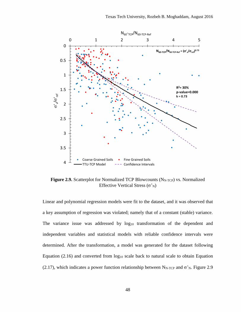
Texas Tech University, Rozbeh B. Moghaddam, August 2016
48
Figure 2.9. Scatterplot for Normalized TCP Blowcounts (NN-TCP) vs. Normalized
Effective Vertical Stress (’N)
Linear and polynomial regression models were fit to the dataset, and it was observed that
a key assumption of regression was violated; namely that of a constant (stable) variance.
The variance issue was addressed by log10 transformation of the dependent and
independent variables and statistical models with reliable confidence intervals were
determined. After the transformation, a model was generated for the dataset following
Equation (2.16) and converted from log10 scale back to natural scale to obtain Equation
(2.17), which indicates a power function relationship between NN-TCP and ’N. Figure 2.9
0
0.5
1
1.5
2
2.5
3
3.5
4
0 1 2 3 4 5
' v
/' re
f
N60-TCP/N60-TCP-Ref
Coarse Grained Soils Fine Grained Soils
TTU-TCP Model Confidence Intervals
R2= 30% p-value=0.000k = 0.73
N60-TCP/N60-TCP-Ref = ('v/ref)0.73

Texas Tech University, Rozbeh B. Moghaddam, August 2016
49
presents the model fitted to the dataset based on Equation (2.16) illustrated by the solid line
including its corresponding 95% confidence intervals (CI) identified by dashed lines.
𝑙𝑜𝑔10(𝑁𝑁−𝑇𝐶𝑃) = 0.73 𝑙𝑜𝑔10(𝜎′𝑁) (16)
(𝑁60−𝑇𝐶𝑃
𝑁60−𝑇𝐶𝑃−𝑅𝑒𝑓) = (
𝜎′𝑣
𝜎𝑟𝑒𝑓)
0.73
(17)
Overburden correction factor CN-TCP
From the combination of Equations (2.13) and (2.17), the overburden correction factor for
the TCP test (CN-TCP) is obtained as follows.
𝐶𝑁−𝑇𝐶𝑃 =1
(𝜎′
𝑣
𝜎𝑟𝑒𝑓)
0.73 (2.18)
Equation (2.18) represents a power function which is the recommended overburden
correction factor for the TCP tests with a power (k) of 0.73. To provide context, the
expression determined for CN-TCP in this study was compared to the models published for
CN for SPT shown in Table 2.2, by plotting the effective vertical stress (’v) versus CN, as
shown in Figure 2.10.
Figure 2.10 illustrates the relationship between the effective vertical stress and the
overburden correction factors published for the SPT compared to the overburden correction
factor for the TCP presented in this paper. The relationship for the TCP test is shown with

Texas Tech University, Rozbeh B. Moghaddam, August 2016
50
the solid line with 95% CI dashed lines. From the comparison, it is noted that the
overburden correction factors presented by other researchers for the SPT data vary between
0.35 and 2.1; whereas, the correction factors for the TCP test range from 0.4 to 3.05. It is
inferred that the broad spectrum of the overburden correction factor for the TCP test may
be associated with the fact that the TCP test data analyzed in this study included both fine-
grained and coarse-grained soils whereas the factors developed for the SPT included
coarse-grained soils only.
Figure 2.10. Effective Vertical Stress (’v) versus CN for TCP and SPT
0
50
100
150
200
250
300
350
400
0 0.5 1 1.5 2 2.5 3 3.5
'v
(kP
a)
CN
Peck et. al. (1974)
Seed (1976)
Tokimatsu (1983)
Skempton(1986) DR=40-60%
Skempton(1986) DR=60-80%
Skempton (1986) OC Sand
Liao Whitman (1986)
Clayton (1993)
TTU-CN-TCP
TTU-CN-TCP-Confidence Intervals

Texas Tech University, Rozbeh B. Moghaddam, August 2016
51
OTHER FACTORS THAT MAY INFLUENCE TCP TEST HAMMER EFFICIENCY
Analyses of the TCP test data, observations of the TCP field procedure, and comments in
the technical literature suggest that factors other than those corrected for herein could create
variability in the NTCP. Four additional factors – drill rod size, type of soil, drilling fluid,
and depth – were identified and analyzed to explore their influence on TCP hammer
efficiency.
Statistical analyses using ANOVA were performed using SAS9.3 (2015) and Minitab
17.3.1 (2016) to study the effect of drill rod size, type of soil, drilling fluid, and depth, on
the hammer efficiency. For this process, the hammer efficiency was considered as
dependent variable and all other factors as independent variables/factors. This ANOVA
also tested for interactions between these factors. A three-way interaction is observed
between drilling fluid, soil type, and depth. This implies that each of these are associated
with hammer efficiency. Furthermore, drill rod size is involved in two significant two-way
interactions, which implies that it is also associated with hammer efficiency.
Results from these analyses indicate that a statistically significant relationship exists
between the identified factors and hammer efficiency, but because the data were not
obtained from a controlled experiment, the exact nature of these relationships could not be
determined. Hence, to develop correction factors that account for all the variables
influencing TCP hammer efficiency, additional study is required where the research design
allows each factor to be analyzed independently.

Texas Tech University, Rozbeh B. Moghaddam, August 2016
52
SUMMARY AND CONCLUSIONS
This paper presents TCP hammer efficiency data, rod length correction factors, and
overburden correction factors for instrumented TCP tests completed in coarse-grained and
fine-grained soils. Other factors that may influence TCP hammer efficiency were also
identified.
A dataset of 293 TCP tests comprising 251 tests completed in soils and 42 in IGM/Rock
was compiled for this study. From the 293 TCP tests, 135 tests were instrumented to obtain
energy measurements using the SPT Analyzer, with 119 instrumented tests in soils and 16
instrumented tests in IGM/Rock. An adjusted dataset of 251 TCP tests were considered for
the development of overburden correction factors for the TCP test in soils. A total of 119
instrumented TCP tests in soils were used for the analysis corresponding to the rod length
correction factors.
Undifferentiated efficiency values range from 74% to 101% with mean of 89% and COV
of 5.07 associated with TCP blowcounts ranging from 3 to 100 with an average of 38
blows/30-cm and measured at depths ranging from 3-m (5-ft) to 30-m (100-ft), average 13-
m (43-ft). TCP hammer efficiency values ranged from 74% to 101% with a mean of 90%
and COV of 4.85 for coarse-grained soils, and from 77% to 97% with an average of 88%
and COV of 5.13 for fine-grained soils. These TCP hammer efficiency values are similar
in range but about 7% higher on average than efficiency values for automatic SPT hammers
published in the literature.

Texas Tech University, Rozbeh B. Moghaddam, August 2016
53
Rod length correction factors for the TCP hammer efficiency (CR-TCP) were developed by
creating a non-linear model based on statistical analyses. Rod length correction factors
ranging from 0.90 and 1.00 for undifferentiated data were determined and recommended
for the TCP test.
In a separate set of analyses, the relationship between N60-TCP and soil overburden pressure
was analyzed. Correction factors for the overburden pressure for the TCP test (CN-TCP) were
developed and normalized to a reference stress (100 kPa). The CN-TCP expression
recommended in this paper is a power function with k= 0.73, and this is generally in
agreement with the CN expressions published for the SPT.
Although the TCP test is in some ways similar to the SPT, the two tests are not the same,
even though results from both tests are used to design deep foundations. Therefore, it
makes sense to take steps to ensure reliable data. In case of the SPT, the corrections for
raw blowcount data are well established; whereas, for the TCP test, up until now, no
published corrections exist. The work presented in this paper is intended as an initial step
to further refine the TCP-based design to achieve more reliable design of deep foundations.

Texas Tech University, Rozbeh B. Moghaddam, August 2016
Note 3: Moghaddam R.B., Jayawickrama, P.W., Lawson, W.D., Seo H., Surles, J.G. (2016), “Evaluation of
Predicted Validity of the Texas Cone Penetration Design Charts for Deep Foundations based on Full Scale
Load Tests”, Journal of Performance of Constructed Facilities
54
CHAPTER III
EVALUATION OF PREDICTED VALIDITY OF THE TEXAS CONE PENETRATION
DESIGN CHARTS FOR DEEP FOUNDATIONS BASED ON FULL SCALE LOAD
TESTS3
ABSTRACT
This study presents a quantitative and a qualitative evaluation of the predictive validity of
the Texas Cone Penetration (TCP) foundation design charts. Allowable measured total
capacities determined from results of full-scale load tests were compared to allowable
predicted total capacities determined from TCP foundation design charts. The final dataset
compiled for this study consisted of 60 full scale load testes comprising 33 driven piles and
27 drilled shafts. Allowable measured capacities were determined using strength-based and
serviceability-based models. Results from analyses suggested that it is apparent that
different performance assessment criteria leads to different conclusions regarding the
predictive validity of the TxDOT TCP method for deep foundation design. The allowable
predicted total capacity determined from the TCP foundation design charts could be
considered to be reasonable based on a strength-based model, moderately over-
conservative, to over-conservative according to serviceability-based models. Further, it
was observed that as the level of tolerable settlement is increased, the interpretation of the
TCP foundation design charts becomes even more conservative.

Texas Tech University, Rozbeh B. Moghaddam, August 2016
55
INTRODUCTION
This paper presents an evaluation of the predictive validity of the Texas Department of
Transportation (TxDOT) Texas Cone Penetration (TCP) foundation design charts by
comparing the allowable predicted total capacity (determined from the TCP foundation
design charts) to the allowable measured total capacity (obtained from full scale load tests)
for driven piles and drilled shafts in soils.
The TCP field test procedure is introduced, and its associated foundation design charts are
presented. The application and use of the TCP charts for the design of deep foundations is
discussed in detail. The effort associated with field data collection including geotechnical
borings using the TCP tests is described, followed by a detailed discussion of the
development of the project dataset. Two different approaches were used to determine the
allowable measured total capacity from results of full-scale load tests. The first approach
was a strength-based method where the total capacities at the ultimate limit state were
determined from the load-settlement curves and then divided by a Factor of Safety (FS) to
determine the allowable measured total capacity. The second approach was serviceability-
based where loads corresponding to tolerable settlements were identified from the load-
settlement curves, and these loads were considered as the allowable measured total
capacity.
After determining the allowable measured total capacity and the allowable predicted total
capacity, these data were analyzed based on (1) a qualitative evaluation where all data were

Texas Tech University, Rozbeh B. Moghaddam, August 2016
56
plotted and compared to in reference to the line of equality, and (2) a quantitative evaluation
where statistical analysis and linear regression models were developed to analyze the
relationship between allowable measured total capacity and the allowable predicted total
capacity.
The TCP test and its associated foundation design charts have been used for the design of
driven pile and drilled shaft foundations that support tens of thousands of bridges and other
major transportation infrastructure throughout Texas for over 60 years.
As would be expected with its Texas roots, the TCP test has seen extensive application
throughout Texas to evaluate subsurface materials ranging from very soft clays, to shales
and fractured limestones, to hard rock. However, the use of TCP test and its associated
design charts are not limited to Texas practice only. Because of its applicability to a wide
range of geomaterials, the TCP test has been used not only throughout the United States
but also for international projects. According to FHWA (2016) Texas currently maintains
over 53,000 bridges in the National Bridge Inventory, and most of these bridges plus other
transportation infrastructure in Texas are supported by foundations designed in accordance
with the TCP method. Also, since Oklahoma DOT adopted the TCP test in the 1970s, the
TCP method has been used for the design of the foundations for most of the 23,000 bridges
in Oklahoma’s inventory. Collectively this indicates that over 12% of the nation’s bridges
are associated with the TCP test. The TCP test is discussed in NCHRP Synthesis 360
(Turner 2016), and owing to competitive opportunities for Texas’ major transportation

Texas Tech University, Rozbeh B. Moghaddam, August 2016
57
infrastructure projects, geotechnical practitioners and academics nationwide have had
occasion to learn about and use the TCP test. Recently, a comprehensive research program
in Missouri evaluated a modified version of the TCP test for bridge foundation design
applications using LRFD concepts (Loehr et al. 2011). The TCP test was introduced to an
international audience during a workshop sponsored by the Port and Airport Research
Institute of Japan, and the application of the method for the design of deep foundations
was discussed as part of Advance in Deep Foundations in Japan, (Vipulanandan, C. 2007).
Furthermore, the TCP test has been used in Korea for field explorations associated with a
bridge abutment overlying intermediate geomaterials and soft rock where cores would have
been recovered in fragments because of joint structures (Nam et al. 2013). In light of the
preceding, the scope of the TCP test and its associated foundation design charts is
significant well beyond its regional origins.
THE TXDOT TEXAS CONE PENETRATION TEST
Description of the TCP test
The TCP field test is a dynamic penetration test which assesses the strength of the geologic
material encountered during geotechnical exploration. This test method is considered to be
a simple, rugged, yet sufficiently reliable tool for characterization of a broad range of
geologic material that range from clays, sands, intermediate geomaterials and hard rock.
The TCP test method is documented as TxDOT Designation Tex-132-E, “Test Procedure
for Texas Cone Penetration” (TxDOT 1999). It uses a 77.0-kg (170-lb) hammer with 0.61-

Texas Tech University, Rozbeh B. Moghaddam, August 2016
58
m (24-in) drop to force a 7.6-cm (3-in) diameter steel cone into the soil or rock formation,
Figure 3.1.
In current practice, penetration for the TCP test is to be achieved in three separate
increments. The first increment is the seating blows and consists of driving the cone 12
blows or approximately 15-cm (6-in), whichever comes first. The TCP blowcount is then
determined as the sum of the number of blows required to achieve the second and third 15-
cm (6-in) increments. The total blowcount or (NTCP) corresponding to 30-cm (12-in)
penetration is used to obtain design parameters. In very hard materials such as rock and
intermediate geomaterials (IGM), after the proper seating process, the cone is driven 100
blows and the penetration values for the first and second 50 blows are recorded, with the
NTCP value reported as centimeters (inches) of penetration per 100 blows.
TCP Design Charts
The axial load capacity of a deep foundation is governed by the shear strength of the
geomaterial supporting the foundation at both shaft and base level. Therefore, reliable
assessment of the shear strength of the geomaterial is necessary for accurate prediction of
the axial load of the foundation.

Texas Tech University, Rozbeh B. Moghaddam, August 2016
59
(a) Conical Driving Point (TxDOT 1999) (b) Field Application
Figure 3.1. TCP Test Conical Driving Point (TxDOT, 1999)
One of the unique aspects of the TCP test is that it was developed to evaluate all types of
subsurface materials using a consistent in-situ field test method (TxDOT 2012). Other field
procedures such as the SPT and the Cone Penetration Test are only applicable for a
particular subset of geomaterials, but the TCP test can be used in all materials from soft
clays to dense sands to intermediate geomaterials and rock (TxDOT 2000).
The 1956 edition of the Foundation Exploration and Design Manual provide a series of
correlation curves illustrating shear strength estimation based on NTCP. These correlation
curves were based on relationships established between TCP test data and laboratory-
measured shear strength. To obtain soil strength parameters for this purpose, undisturbed
samples were collected and tested using the triaxial test procedure (THD 1956). Based on
data obtained from field and laboratory studies, correlation charts between NTCP and
foundation capacities were developed and published in two separate sets of design charts.
The first set was developed for soils with TCP blowcounts less than 100 per 30-cm (12-

Texas Tech University, Rozbeh B. Moghaddam, August 2016
60
in); whereas, the second set was for geomaterials with blowcounts greater than 100 blows
per 30-cm (12-in) (i.e. penetration per 100 blows). Figure 3.2 presents the current version
of the TCP foundation design charts for soil as published in the 2012 TxDOT Geotechnical
Manual (TxDOT 2012).
Deep foundations such as driven piles and drilled shafts derive their axial load capacity
from both shaft resistance (also referred to as skin resistance or skin friction in literature)
and base resistance (also referred to as toe bearing resistance or point bearing resistance in
literature). The TxDOT’s Geotechnical Manual TxDOT (2012) refers to these resistances
as skin friction and point bearing, respectively. The manual provides two separate sets of
charts, one set to determine allowable skin friction based on measured TCP blow count and
another set to determine allowable point bearing resistance. Figure 3.2 shows the design
charts used for soil materials, i.e. materials in which blowcounts per 300-mm (12-in) is less
than 100. The TCP foundation design charts reflect the allowable stress design (ASD)
philosophy and present allowable strength values corresponding to a Factor of Safety (FS)
of 2.0. Furthermore, it can be seen that these design charts are categorized based on soil
classification where separate correlations are provided for fat clay (CH), Lean Clay (CL),
Clayey Sand (SC), and OTHER soils. According to the design procedure, any soil
calssified as SP, SW, SM, and ML is considered as OTHER category.

Texas Tech University, Rozbeh B. Moghaddam, August 2016
61
(a) (b)
Figure 3.2. Design charts representing (a) allowable unit shaft resistance and (b)
allowable unit base resistance vs. TCP blows/30-cm (12-in), (TxDOT, 2012)
From Figures 3.2(a) and 3.2(b) it is noted that the soil constants are reported for materials
softer than 100 blows per 300-mm (12-in) of penetration. These constants represent the
inverse of the slope of the allowable capacity models and the slopes vary based on soil
classification. From the nature of the TCP chart for the shaft resistance it is noted that all
predictive models present a maximum blowcount value beyond which the resistance value
becomes constant. For example, in Figure 3.2(a) the model for fat clays (CH) reports
varying unit shaft resistance NTCP =5 to NTCP =70 blows/ 300-mm (12-in), and constant
shaft resistance of 134-kPa (1.4-tsf) for blowcounts beyond 70 blows.
0.0
0.1
0.2
0.3
0.4
0.5
0.6
0.7
0.8
0.9
1.0
1.1
1.2
1.3
1.4
1.5
0 10 20 30 40 50 60 70 80 90 100
S -
Allo
wab
le S
kin
Fri
ctio
n (
tsf)
wit
h F
.S. =
2.0
Texas Cone Penetrometer (NTCP)- Blows/12-in
CH CLSC
OTHER
CH 50
CL 60
SC 70
OTHER 80
S = N/C
C (Constant)
Note: Apply soil reduction factor for drilled shaft design.
0.0
0.5
1.0
1.5
2.0
2.5
3.0
3.5
4.0
4.5
5.0
5.5
6.0
6.5
0 10 20 30 40 50 60 70 80 90 100
Pb
-A
llow
able
Po
int
Bea
rin
g (t
sf)
wit
h F
.S. =
2.0
Texas Cone Penetrometer (NTCP)- Blows/12-in
CH
CL
SC
CH 19.5
CL 16.6
SC 16.3
OTHER 18.6
S = N/C
C (Constant)

Texas Tech University, Rozbeh B. Moghaddam, August 2016
62
TCP Design Method for Deep Foundations
In the design of deep foundations the total resistance (Qt) is the sum of the shaft (Qs) and
base (Qb) resistances. For the TCP method, the total resistance is expressed in function of
unit shaft (qs) resistance, foundation surface area (As), unit base resistance (qb), and
foundation base area (Ab), Equation (3.1).
𝑄𝑡 = 𝑞𝑠𝐴𝑠 + 𝑞𝑏𝐴𝑏 (3.1)
For a TCP-based design, the unit shaft and unit base resistance values are directly from the
TCP design charts. The main parameters required to determine these resistances are the
TCP test blowcount number (NTCP) and the type of soil described based on Unified Soil
Classification System (USCS) group symbol.
The allowable predicted total capacity for driven piles and drilled shafts compiled for this
study was calculated following the guidelines recommended in the Geotechnical Manual
(TxDOT 2012). Two capacity adjustments are specified for the TCP-based design of deep
foundations. The first adjustment is the disregard depth which applies to all type of
foundations and refers to the portion of shaft capacity neglected during design. According
to the Geotechnical Manual (2012), the shaft resistance from the ground surface to a depth
of 1.5-m (5-ft) to 3.0-m (10-ft) will be disregarded, irrespective of whether the deep
foundation will be installed over non-water crossing or over stream crossing. The second
capacity adjustment is the application of a soil reduction factor of 0.7 to the shaft resistance

Texas Tech University, Rozbeh B. Moghaddam, August 2016
63
for the design of drilled shafts. This reduction factor is recommended for use in order to
account for the soil disturbance during the drilling procedure.
The allowable predicted total capacities presented in this study include the soil reduction
factor of 0.7 for the determination of predicted shaft capacity of drilled shafts. The
disregard depth is usually applied to design to account for possible long-term scours. In the
case of this study, predicted capacity is compared to measured capacity from full-scale load
tests where a design assumption such as the disregard depth is not applicable.
RESEARCH DESIGN AND METHOD
Development of the Dataset
The dataset for this study was compiled based on available load test projects from
TxDOT’s historical archive supplemented by projects from neighboring states. TCP boring
data corresponding to full-scale load test projects retrieved from TxDOT’s historical
archive were identified and recorded. For the non-TxDOT projects, new geotechnical
borings using the TCP test method were completed.
TxDOT Historical Archive. Over a period of 50 years, the TxDOT Bridge Division
compiled an archive of load tests completed for driven piles and drilled shafts projects at
various locations in Texas. The TxDOT archive was reviewed in detail and organized
according to (1) availability of TCP data, (2) full scale load test information, and (3)

Texas Tech University, Rozbeh B. Moghaddam, August 2016
64
pertinence to this particular study. Based on this organization, a preliminary dataset was
compiled comprising 31 load test projects in soils for driven piles and 15 load test projects
in soils for drilled shafts, including their corresponding TCP data.
Non-TxDOT Full Scale Load Tests. With the objective of supplementing the TxDOT
historical archive, available load test project sites located in Missouri, Arkansas, Louisiana,
and New Mexico were identified and, at each site, new geotechnical borings with TCP tests
were completed in accordance with the guidelines found in the TxDOT Geotechnical
Manual. All TCP tests were carried out at 1.5-m (5-ft) intervals, starting at a depth of 1.5-
m (5-ft) below the ground surface, and ending at the maximum depth of boring. Disturbed
samples were collected using either SPT split-spoon or thin-walled tube samples obtained
directly below the TCP test without having cleaned out the borehole. These samples were
used for identification and classification of the subsurface materials associated with the
TCP test. After field data collection, two load test projects for driven piles and 12 load test
projects for drilled shafts were added to the preliminary dataset.
From this work, the final dataset compiled for this study consisted of 60 full scale load tests
comprising 33 driven piles and 27 drilled shafts in soils. Driven piles selected for this
project were precast square concrete piles ranging in width from 360-mm (14-in) to 510-
mm (20-in) with embedment lengths varying between 5-m (15-ft) and 25-m (84-ft). For
the drilled shafts, the diameters ranged from 460-mm (18-in) to 1830-mm (72-in) with total

Texas Tech University, Rozbeh B. Moghaddam, August 2016
65
length varying between 6-m (20-ft) and 30-m (99-ft). The final dataset is summarized in
Table 3.1 for driven piles and Table 3.2 for drilled shafts.
As previously mentioned, the primary objective of this study was to evaluate the predictive
validity of the TCP foundation design method based on a comparison between the
allowable predicted total capacity (𝑃𝑎𝑃) and the allowable measured total capacity (𝑃𝑎
𝑀). To
achieve this evaluation, the compiled dataset was further developed to obtain 𝑃𝑎𝑃 from
results of TCP borings, and 𝑃𝑎𝑀 from results of full scale load tests.
Allowable Predicted Total Capacity (𝑷𝒂𝑷)
Allowable predicted total capacity, 𝑃𝑎𝑃 values for driven piles and drilled shafts were
calculated following the design procedure specified by the TxDOT’s Geotechnical
Manual. For this purpose, a synthesized soil profile showing the stratigraphy and NTCP per
strata was generated from geotechnical TCP borings for each load test project. Figure 3.3
illustrates an example of the synthesized soil profile and the average NTCP profile developed
for Case No. 23 of drilled shafts. Then, with the average NTCP, the type of soil, and using
Figure 3.2, the allowable unit shaft and the allowable unit base resistance are determined.
Further, multiplying these unit resistances by their corresponding area (i.e. shaft area and
base area) and summing the total shaft and total base capacity, the allowable predicted total
capacity (𝑃𝑎𝑃) is determined.

Texas Tech University, Rozbeh B. Moghaddam, August 2016
66
Figure 3.3. Illustrative example of determining 𝑃𝑎𝑃 for Case No. 23 of drilled shafts
For the Case No. 23 shown in Figure 3.3, and following the above described process, an
allowable total shaft capacity of 2893-kN (650-Kips) and an allowable total base capacity
of 1073-kN (241-kips) were determined. For the calculation of shaft capacity for the design
of drilled shafts, the TxDOT Geotechnical Manual specifies a soil reduction factor of 0.7.
After applying the reduction factor, a total reduced shaft capacity of 2025-kN (455-Kips)
was obtained. Summing up the total reduced shaft capacity and the total base capacity, an
allowable predicted total capacity of 3000-kN (675-kips) was determined. This process
was completed for all driven piles and drilled shafts included in the compiled dataset. Table
18
16
13
16
22
51
1291
49
79
91
100
0
1.5
3
4.5
6
7.5
9
10.5
12
13.5
15
16.5
18
19.5
21
0 10 20 30 40 50 60 70 80 90 100 110 120 130
Dep
th (
m)
NTCP (Blows/30-cm)
Full
Scal
e L
oad
Te
st-
Dri
lled
Sh
aft,
Dia
me
ter=
16
80-
mm
TCP-Boring
CL
ML (OTHER)
SM (OTHER)
Average NTCP = 17
Average NTCP = 90
SM (OTHER)
NTCP = 18
Average NTCP = 70
NTCP = 51
NTCP = 12 SM (OTHER)
SM (OTHER)

Texas Tech University, Rozbeh B. Moghaddam, August 2016
67
3.1 summarizes the results obtained from for driven piles and while Table 3.2 provides the
results obtained for drilled shafts.
In addition to allowable total capacities, the predominant soil for each load test was
identified based on percent of contribution to the total capacity. The predominant soil type
was then categorized as either fine or coarse grained soil. The soil type corresponding to a
percentage greater than 50% of contribution to the total capacity was considered as the
predominant soil. For this selection, first, the predominant source of capacity was
identified. If the predominant source of resistance was the base of the foundation, then the
material below the base was selected as the predominant soil. In cases where the
predominant source of resistance was the shaft, then the highest percentage of contribution
from the soil type was selected as the predominant soil. For example, for the Case No. 23
shown in Table 3.2, the predominant source of total capacity is the shaft with 70% of
contribution to the 𝑃𝑎𝑃 and the predominant soil contributing to the shaft capacity is coarse
grained soil. Therefore, the predominant soil was considered as coarse-grained soil.
Allowable Measured Total Capacities
To investigate the predictive capability of the TCP design charts, the design outcome from
these charts (i.e. allowable predicted total capacity) must be compared to allowable
measured total capacity. For this purpose, the ultimate capacity is first determined from the
load-settlement curves and then divided by an appropriate factor of safety following the
Allowable Stress Design (ASD) methodology. According to TxDOT (2012) Geotechnical

Texas Tech University, Rozbeh B. Moghaddam, August 2016
68
Manual, TCP design charts for materials with less than 100 blows per 300-mm (12-in) of
penetration (i.e. soils) incorporate a FOS of 2.0.
Several published methods exist for the determination of the ultimate load capacity (Pult.)
from the load-settlement curve. These include Davisson (1975), 5% relative settlement
criterion (Reese and Wright 1977, Reese and O’Neill, 1988), and 10% relative settlement
(Bruce, 1986).
TxDOT Geotechnical Manual (TxDOT 2012) does not provide any recommendation with
regard to ultimate capacity criteria. In fact, a review of 12 research reports and design
manuals published by state DOTs, showed that 11 of the agencies specifies Davisson’s
criterion for the determination of ultimate capacity for driven piles. For drilled shafts, only
three states specified 5% relative settlement to be used as the ultimate capacity criterion.
Based on these results, and the magnitude of settlement in the load-settlement curves
compiled for this study, Davisson’s ultimate capacity criterion was selected was selected
for this study following AASHTO (2012).
Davisson’s criteria considers the elastic compression of the deep foundation element. After
constructing the elastic line, an offset line parallel to the elastic line is plotted. The ultimate
capacity is the load corresponding to the point of intersection of the offset line and the load-
settlement curve. This process is shown in Figure 3.4 (Case No. 23 of drilled shafts).

Texas Tech University, Rozbeh B. Moghaddam, August 2016
69
In engineering design, the allowable load on a structural component may be determined
based on strength-based criteria or serviceability-based (i.e. settlement-based) criteria.
Within the context of deep foundations, the strength-based allowable load capacity can be
defined as ultimate capacity divided by an appropriate factor of safety. Since TxDOT TCP
design charts for soil materials are intended to provide a factor of safety of 2.0, it is
appropriate to use a FS=2.0 in the present analysis. Accordingly, the first set of data was
determined for the allowable measured total capacity, 𝑃𝑎𝑀 by dividing the Davisson’s
ultimate capacity obtained from the load-settlement curves by a FS of 2.0.
The second and third sets of 𝑃𝑎𝑀were serviceability-based, and consisted of loads
corresponding to vertical displacements determined from load-settlement curves. In
geotechnical engineering, deformations presented at the head of the deep foundation are
translated to vertical settlements noted in the superstructure. When settlements are larger
than an established tolerable settlement (tol), then it is considered that the foundation
element has reached a serviceability limit condition, and the performance of the
superstructure is not satisfactory.
The extent of the tolerable displacement may be specified by regulatory agencies such as
AASHTO (2014), it can be determined based on behaviors of similar structures (Roberts
et al. 2010), or it can be calculated based on predictive models. The National Cooperative
Highway Research Program (NCHRP) Report No. 343 (Barker et al. 1991) presents
guidelines and specifications describing allowable total and differential settlement for

Texas Tech University, Rozbeh B. Moghaddam, August 2016
70
transportation structures. According to AASHTO (2014), the tolerable differential
settlement for highway bridges can be evaluated in terms of angular distortions ().
Further, for continuous span and single span bridges, an angular distortion of 0.004 and
0.008 are recommended, respectively. However it is also discussed that these large values
“concerns structural designers, who often limit tolerable movement to one-half to one-
quarter, or one less order of magnitude i.e., 0.004 to 0.0004”, (SHRP2-solutions, 2016).
Zhang et al. (2005) presented wok completed for 50 concrete bridge foundations with
angular distortions ranging from 0.001 to 0.08, where 61% of the tolerable cases (i.e.
acceptable settlement) presented angular distortions smaller than or equal to 0.002.
In an effort to establish tolerable settlements for this study, a detailed review of available
technical documents and construction drawings associated with the compiled dataset was
completed. From this review, the average bridge span length corresponding to the projects
associated with the load test cases was determined. A total of 77 multi-span bridges
supported by driven piles with an average span length of 18-m (60-ft), and 28 multi-span
bridges supported by drilled shafts with an average span of 21-m (70-ft) were identified.
Using the angular distortion value of 0.004 recommended by AASHTO (2014), tolerable
settlements of 72-mm (2.83-in) for driven piles and 84-mm (3.31-in) for drilled shafts were
obtained. These values are in accordance with other published tolerable settlement value
of 51-mm (2-in) reported by Coduto et al. (2011).

Texas Tech University, Rozbeh B. Moghaddam, August 2016
71
Although the tolerable settlements determined based on angular distortion recommended
by AASHTO (2014) ranged from 72-mm (2.83-in) to 84-mm (3.31-in), load settlement
curves compiled for this study did not reach those values of settlement. Based on the dataset
of this study, the vertical displacement values were selected based on the reasonable
assumption that the allowable vertical displacement for foundations supporting bridge
structures will not exceed 6.35-mm (0.25-in) to 12.7-mm (0.5-in). The final dataset
including all four 𝑃𝑎𝑀, and 𝑃𝑎
𝑃 is presented in Table 3.1 for driven piles and Table 3.2 for
drilled shafts.
Figure 3.5 illustrates the load-settlement curve corresponding to the Case No. 23 of drilled
shafts showing Davisson’s line, and loads corresponding to 6.35-mm (0.25-in) and 12.7-
mm (0.5-in) of settlement. The intercept of Davisson’s line with the load-settlement curve
yielded the Davisson’s ultimate capacity value of 6956-kN (156-kips). This value was
further used to determine 𝑃𝑎𝑀 by dividing the value by 2.0 and 3.0 resulting in 3478-kN
(782-kips) and 2320-kN (521-kips), respectively.
To determine 𝑃𝑎𝑀 based on serviceability-based criteria, horizontal lines corresponding to
settlements of 6.35-mm (0.25-in) and 12.7-mm (0.5-in) were plotted from the vertical axis,
and the intercept of these lines with the load-settlement curve yielded the corresponding
loads of 5518-kN (1240-kips) and 6230-kN (1400-kips), respectively.

Texas Tech University, Rozbeh B. Moghaddam, August 2016
72
The process described above for both Davisson’s ultimate capacity criterion and
serviceability criteria, were implemented for all 60 load test projects compiled for the study
presented in this paper.
Figure 3.4. Case No. 23, Davisson’s ultimate Capacity Criterion and Serviceability
Criteria
DATA ANALYSIS
The predictive validity of TCP foundation design charts was evaluated in three separate
analyses: (1) qualitative evaluation of the allowable total capacity of deep foundations
determined from TCP foundation design charts (2) prediction of allowable total capacity
for driven piles, and (3) prediction of allowable total capacity for drilled shafts. A fourth
analysis was attempted where the shaft and base capacity were analyzed separately.
0
10
20
30
40
50
60
70
0 1000 2000 3000 4000 5000 6000 7000 8000
Se
tlle
me
nt -
(
mm
)
Axial load (kN)
(6956, 49)
(6230, 12.7)
(5518, 6.35)
Serviceability Criterion Line, = 12.7-mm
Serviceability Criterion Line, = 6.35-mm

Texas Tech University, Rozbeh B. Moghaddam, August 2016
73
The first comparison consisted of preparing scatterplots of allowable total capacities for
driven piles and drilled shafts to observe the overall prediction trends of the TCP
foundation design model. For all four sets of 𝑃𝑎𝑀, individual scatterplots were generated to
observe the behavior of the data compared to line of equality (i.e. 45° line).
The second and third analyses consisted of evaluating the relationship between the three
expressions of 𝑃𝑎𝑀 obtained from full scale load tests and 𝑃𝑎
𝑃 determined from TCP design
charts using linear regression analysis for driven piles and drilled shafts independently.
These analyses were performed using four subsets of data:
Strength-based Models:
Model-1: Allowable load corresponding to Davisson’s ultimate capacity criteria
divided by a FS of 2.0, 𝑃𝑎−𝐷/2𝑀
Serviceability-based (Performance) Models:
Model-2: Allowable load corresponding to loads at 6.35-mm (0.25-in) of settlement
determined from load-settlement curves, 𝑃𝑎−𝛿=6.35
𝑀
Model-3: Allowable load corresponding to loads at 12.7-mm (0.5-in) of settlement
also determined from load-settlement curves. 𝑃𝑎−𝛿=12.35
𝑀
For the second and third analyses, regression models were fitted to the data and compared
among each other, and to the line of equality. All statistical analyses were performed using
Minitab 17.0 (2016).

Texas Tech University, Rozbeh B. Moghaddam, August 2016
74
Table 3.1. Compiled Dataset for Driven Piles in Soils
Case
No.
Pile Dimensions
Predominant
Source of Total
Capacity (%)
Soil2
𝑃𝑎𝑃
𝑃𝑢𝑙𝑡3 𝑃𝑎−𝐷/2
𝑀 𝑃𝑎−𝛿=6.35
𝑀 𝑃𝑎−𝛿=12.35
𝑀
Width
(mm)
Length1
(m) Shaft Base (kN) (kN) (kN) (kN) (kN)
1 360 9 96% 4% Fine 431 497 248 490 543
2 360 8 97% 3% Coarse 385 1,654 827 1,513 1,682
3 360 7 91% 9% Fine 437 1,161 581 1,068 1,246
4 360 11 96% 4% Fine 808 866 433 823 894
5 510 21 97% 3% Fine 748 2,901 1,450 1,958 2,670
6 380 11 92% 8% Fine 622 1,574 787 1,157 1,647
7 380 10 94% 6% Coarse 677 1,365 682 1,090 1,424
8 410 15 98% 2% Coarse 552 2,297 1,148 1,308 1,709
9 410 13 99% 1% Coarse 984 1,044 522 935 1,090
10 410 13 96% 4% Coarse 523 1,291 646 1,113 1,308
11 410 14 97% 3% Fine 1,241 1,652 826 1,291 1,669
12 410 5 93% 7% Fine 313 1,047 524 979 1,135
13 410 5 93% 7% Fine 236 1,598 799 1,469 1,691
14 410 14 99% 1% Coarse 910 1,304 652 1,068 1,335
15 410 9 98% 2% Fine 669 1,049 525 957 1,090
16 410 9 96% 4% Fine 441 1,344 672 1,224 1,371
17 410 12 96% 4% Fine 466 579 289 445 734
18 380 9 95% 5% Fine 404 1,255 627 1,046 1,357
19 510 23 98% 2% Fine 1,345 1,117 558 1,024 1,126
20 360 8 94% 6% Fine 1,647 1,570 785 1,580 1,780
21 460 10 93% 7% Fine 526 1,580 790 1,139 1,647
22 460 25 89% 11% Fine 642 1,222 611 979 1,224
23 460 14 97% 3% Fine 877 2,406 1,203 1,037 1,059
24 360 8 96% 4% Fine 530 1,122 561 1,068 1,148
25 460 13 95% 5% Coarse 824 1,722 861 1,335 1,736
26 460 13 95% 5% Coarse 824 1,712 856 1,558 1,736
27 460 12 97% 3% Coarse 763 1,519 760 1,291 1,580
28 460 13 95% 5% Coarse 824 2,668 1,334 1,780 2,603
29 460 17 95% 5% Coarse 1,340 3,132 1,566 2,092 3,004
30 510 22 97% 3% Coarse 2,203 3,031 1,515 2,626 3,026
31 510 22 96% 4% Fine 1,568 2,173 1,086 2,181 2,474
32 360 13 99% 1% Coarse 687 1,096 548 979 1,135
33 360 24 98% 2% Fine 1,837 3,014 1,507 1,424 2,359
Note: 1. Embedment Length, 2. Predominant Soil Type 3. Davisson’s Ultimate Capacity Criterion

Texas Tech University, Rozbeh B. Moghaddam, August 2016
75
Table 3.2. Compiled Dataset for Drilled Shafts in Soils
Case
No.
Drilled Shaft
Dimensions
Predominant
Source of Total
Capacity (%) Soil2
𝑃𝑎𝑃 𝑃𝑢𝑙𝑡
3 𝑃𝑎−𝐷/2
𝑀 𝑃𝑎−𝛿=6.35
𝑀 𝑃𝑎−𝛿=12.35
𝑀
Diameter
(cm)
Length1
(m)
Shaft Base
(kN) (kN) (kN)
(kN)
(kN)
1 910 8 70% 30% Fine 2,085 7,958 3,979 3,916 6,008
2 1220 16 76% 24% Coarse 5,461 9,531 4,766 6,853 8,277
3 1220 16 76% 24% Coarse 5,461 9,126 4,563 5,830 7,209
4 1220 16 76% 24% Coarse 5,461 10,633 5,316 6,675 8,240
5 910 18 89% 11% Fine 3,700 7,521 3,761 5,518 6,542
6 610 6 82% 18% Fine 1,009 2,444 1,222 1,780 2,581
7 460 8 84% 16% Fine 402 539 269 534 547
8 460 7 92% 8% Fine 275 491 246 467 512
9 760 7 88% 12% Fine 545 1,157 578 1,024 1,121
10 760 7 88% 12% Fine 545 838 419 757 810
11 760 14 91% 9% Fine 1,114 2,702 1,351 2,314 2,537
12 760 18 90% 10% Coarse 2,280 4,372 2,186 3,783 4,139
13 760 23 96% 4% Fine 1,783 6,058 3,029 5,474 5,919
14 760 14 82% 18% Coarse 3,502 5,344 2,672 3,516 4,406
15 1830 20 76% 24% Coarse 4,423 12,120 6,060 5,474 7,343
16 1220 26 93% 7% Coarse 3,650 10,939 5,470 5,340 7,699
17 1220 27 91% 9% Coarse 3,773 12,019 6,010 5,385 7,521
18 1680 19 84% 16% Fine 3,773 4,931 2,466 3,560 4,228
19 1680 12 85% 15% Fine 2,105 5,120 2,560 3,694 4,094
20 1830 25 87% 13% Fine 4,705 8,405 4,202 6,453 7,120
21 1220 30 92% 8% Fine 4,018 11,176 5,588 5,830 8,277
22 1220 12 23% 77% Fine 1,883 3,756 1,878 2,982 3,427
23 1680 14 70% 30% Coarse 3,000 6,956 3,478 5,518 6,230
24 790 14 89% 11% Coarse 5,067 6,491 3,245 4,450 5,518
25 790 14 89% 11% Coarse 5,108 7,779 3,890 4,984 6,408
26 1220 23 85% 15% Coarse 5,137 8,256 4,128 2,670 4,183
27 810 17 91% 9% Coarse 2,764 6,598 3,299 1,958 3,382
Note: 1. Embedment Length, 2. Predominant Soil Type 3. Davisson’s Ultimate Capacity Criterion
Qualitative Evaluation
To facilitate qualitative evaluation of the predictive capabilities of the TCP foundation
design charts, scatterplots were generated for all the data and compared to line of equality,

Texas Tech University, Rozbeh B. Moghaddam, August 2016
76
Figure 3.5. To create these plots, the ultimate 𝑃𝑎𝑀
determined for each model for both driven
piles and drilled shafts were used to generate an undifferentiated scatterplot.
Figures 5(a) correspond to the strength-based model where the ultimate deep foundation
capacity was interpreted using Davisson’s criterion and the allowable measured total
capacities were determined by dividing the ultimate capacity value by a FS of 2.0. Data
points above the equal prediction line (i.e., 1:1 Line) are conservative (𝑃𝑎𝑀 > 𝑃𝑎
𝑃) and data
points below the equal prediction line are unconservative (𝑃𝑎𝑀 < 𝑃𝑎
𝑃). However, this does
not mean that the performance of the foundation is in jeopardy. It is important to note that
the ultimate capacity criterion is not necessarily a physical event but rather a defined
computational condition (Foye et al. 2009). For example, in the case of a full scale load
test completed for a deep foundation, the plunging load can be considered as the physical
event of ultimate limit state but it is different from the load determined from accepted
ultimate criteria (e.g. Davisson’s, 5% or 10% relative settlement) established as the
computational condition. Therefore, unconservative design does not necessarily lead to
poor performance. This is better illustrated with the serviceability-based models in the
following paragraph.
From Figure 3.5(a) it is noted that, even though significant scatter exists, the data points
are approximately evenly split above and below the 1:1 line when a FS of 2.0 is used. In
this plot 34 data points representing slightly more than 50% of the dataset plotted below
the 1:1 line. Based on these findings it is reasonable to conclude that overall, the allowable

Texas Tech University, Rozbeh B. Moghaddam, August 2016
77
total capacity predictions made by using the TCP design procedure agree well with
measured values. In other words, the probability that the actual capacity will be higher
than that predicted by the design charts is about the same as the probability that it will be
lower. Accordingly, the design procedure can be expected to yield a bias value close to
unity. However, because of the significant scatter observed in the data, one cannot
conclude that the predictive capabilities of the TCP design procedure as strong. At the
same time, it is important to point out that it would not be reasonable to attribute all of the
scatter observed to inadequacies of the TCP test method. Other factors such as differences
in load testing procedures used (top down versus O-cell, loading rates, time lag between
installation of test foundation and load testing), measurement errors during testing,
differences in foundation construction/installation methods (pile driving, use of slurry
versus dry hole installation used for drilled shafts) would have also contributed to such
scatter.

Texas Tech University, Rozbeh B. Moghaddam, August 2016
78
(a) Scatterplot for Model-1: 𝑃𝑎−𝐷/2
𝑀
(b) Scatterplot for Model-2: 𝑃𝑎−𝛿=6.35
𝑀 (c) Scatterplot for Model-3: 𝑃𝑎−𝛿=12.35
𝑀
Figure 3.5. The relationship between 𝑃𝑎𝑀 and 𝑃𝑎
𝑃 compared to an equal prediction line
0
1000
2000
3000
4000
5000
6000
7000
0 1000 2000 3000 4000 5000 6000 7000
Allo
wable
Pre
dic
ted T
ota
l C
apacity (
kN
)
Allowable Predicted Total Capacity (kN)
Model-1
Driven Piles
Drilled Shafts
Conservative
Unconservative
0
1000
2000
3000
4000
5000
6000
7000
0 1000 2000 3000 4000 5000 6000 7000
Allo
wa
ble
Pre
dic
ted
To
tal C
ap
acity (
kN
)
Allowable Predicted Total Capacity (kN)
Model-2
Driven Piles
Drilled Shafts
Conservative
Unconservative
0
1000
2000
3000
4000
5000
6000
7000
0 1000 2000 3000 4000 5000 6000 7000
Allo
wa
ble
Pre
dic
ted
To
tal C
ap
acity (k
N)
Allowable Predicted Total Capacity (kN)
Model-3
Driven Piles
Drilled Shafts
Conservative
Unconservative

Texas Tech University, Rozbeh B. Moghaddam, August 2016
79
For the serviceability-based models, it is observed that for a tolerable settlement of 6.35-
mm (0.25-in), Figure 3.5(b), approximately 7 data points are below the line of equality.
For a tolerable settlement level of 12.7-mm (0.5-in), Figure 3.5(c), only 2 points are below
the equal prediction line (one point for driven piles and one corresponding to drilled shafts).
From these observations, it is apparent that different allowable capacity criteria leads to
different conclusions regarding the validity of the TxDOT TCP method for deep foundation
design. The allowable predicted total capacity determined from the TCP foundation design
charts could be considered to be reasonable based on Model-1, conservative based on
Model-2, and over-conservative for Model-3. In general, this suggests that serviceability-
based interpretation of the TCP foundation design charts (which is closely associated with
observed structure performance) will be conservative as shown by both Models 2 and 3.
As previously described, Coduto et al. (2011) reported a tolerable settlement value of 51-
mm (2-in) for the serviceability conditions. Similarly, angular distortions specified by
AASHTO (2014) yielded tolerable settlements of 72-mm (2.83-in) for driven piles and 84-
mm (3.31-in) for drilled shafts. Collectively, for higher magnitude of tolerable settlements
the TCP foundation design charts will predict the total capacity of the foundation in a more
conservative manner.

Texas Tech University, Rozbeh B. Moghaddam, August 2016
80
Statistical Analysis
This section presents the analyses completed for driven piles and drilled shafts where the
predictive validity of the TCP foundation design charts are evaluated quantitatively. For
each subset of data, the relationship between 𝑃𝑎𝑀 and 𝑃𝑎
𝑃 was identified in terms of a
regression model and these models were compared to the line of equality (i.e. 45° line).
Linear regression analyses were performed with the 𝑃𝑎𝑀 considered as the response variable
and the 𝑃𝑎𝑃 as the predictor. Prior to each regression analysis, the data were analyzed to
ensure that all assumptions for a simple linear regression analysis were met (i.e. normality,
homoscedasticity, etc.). Linear models were determined following the form of Equation
(3.2) where o and 1 are the intercept and the slope of the regression model, respectively.
𝑃𝑎−𝑚𝑒𝑎𝑠 = 𝛽0 + 𝛽1𝑃𝑎−𝑝𝑟𝑒𝑑 (3.2)
For each model, the existence of a relationship between 𝑃𝑎𝑀
and 𝑃𝑎𝑃 was confirmed by p-
values and the strength of the relationship was assessed by the coefficient of determination
(R2).
The regression models were compared to the equal prediction line to observe whether the
equal prediction line was completely within the confidence boundaries of the regression
model. The confidence intervals (CI) for the regression model were considered as the set
of all reasonable linear models suggested by the data.

Texas Tech University, Rozbeh B. Moghaddam, August 2016
81
RESULTS
Statistical analyses were performed to observe whether the predominant soil type had a
statistically significant impact on the regression models developed for undifferentiated data
by type of soil. For the compiled dataset, the predominant soil was categorized as fine and
coarse grained soils and it was assigned based on percentage of contribution of the soil
type to the predicted allowable total capacity of the foundation.
The compiled dataset showed that the predominant soil for 13 driven piles and 13 drilled
shafts was categorized as coarse grained soil, and the remaining 20 driven piles and 14
drilled shafts had fine grained soils as the predominant soil. An Analysis of Covariance
(ANCOVA) was performed where 𝑃𝑎𝑀 was identified as the response variable, 𝑃𝑎
𝑃 as
predictor (covariate), and the type of soil as the categorical predictor (factor). Results from
these analyses showed that with a p-value greater than 0.05 (i.e. 0.681 for driven piles and
0.223 for drilled shafts) a regression model fitted for fine grained soil did not have a
statistically-significant difference from the model for coarse grained soil. Therefore all
analyses were completed for undifferentiated soil data, but differentiated by foundation
type.

Texas Tech University, Rozbeh B. Moghaddam, August 2016
82
Regression Models
Linear regression analyses were completed to further explore the relationship between 𝑃𝑎𝑀
and 𝑃𝑎𝑃 for each type of foundation. Regression models were fitted to the corresponding
data for driven piles, Figure 3.6, and drilled shafts, Figure 3.7, following the form of
Equation (3.2). In these figures, the regression models are shown as solid lines, the 95%
confidence interval (CI) with dashed lines, and the equal prediction line with dash-dot lines.
Figure 3.6. Scatterplot and fitted model, Driven Piles
For driven piles, Figure 3.6, the model shifts from under-predicting to over-predicting at
approximately 800-kN (180-kips). Further, it is noted that only a small portion of the equal

Texas Tech University, Rozbeh B. Moghaddam, August 2016
83
prediction line plots within 95% CI boundaries indicating that the line of equality is not a
plausible model that could describe the relationship between 𝑃𝑎𝑀 and 𝑃𝑎
𝑃.
The regression model includes and intercept greater than zero. This is not an indication that
for a 𝑃𝑎𝑃 = 0 the 𝑃𝑎
𝑀 would have a value. This suggests that the regression line is
extrapolating through the region where data did not exist (region comprehended
between 𝑃𝑎𝑃 = 250-kN and 𝑃𝑎
𝑀= 750-kN). This indicates that the true relationship
between 𝑃𝑎𝑀 and 𝑃𝑎
𝑃 is actually nonlinear in that region, but appears linear where data points
exist.
In the case of drilled shafts, linear regression models were fitted to the dataset and it was
observed that the fitted model performs much better, Figure 3.7. The model still slightly
over-predicts for 𝑃𝑎𝑃 greater than 4000-kN (900-kips), but the equal prediction line plots
within the 95% CI boundaries for the regression model indicating an acceptable
comparison between the regression model and the equal prediction line.

Texas Tech University, Rozbeh B. Moghaddam, August 2016
84
Figure 3.7. Scatterplot and fitted model, Drilled Shafts
Side-by-Side Comparison of all Measured Capacity Models
As previously described, three models were considered for the performance evaluation of
the TCP foundation design charts. Models 1 was strength-based and Models 2 and 3 were
serviceability-based. For all these models, the relationship between 𝑃𝑎𝑀 and 𝑃𝑎
𝑃 was
investigated, and regression models were developed for driven piles, Figure 3.8, and drilled
shafts, Figure 3.9. These regression lines were plotted side-by-side for comparison
purposes. The existence and the strength of the relationship between 𝑃𝑎𝑀 and 𝑃𝑎
𝑃 were
evaluated based on p-values and R2 determined for driven piles, Table 3.3, and drilled
shafts, Table 3.4.

Texas Tech University, Rozbeh B. Moghaddam, August 2016
85
Table 3.3. Regression line equation with p-value and R2, Driven Piles
Model Regression Equation p-value R2 (%)
1 𝑃𝑎−𝐷/2𝑀 = 455+0.431𝑃𝑎
𝑃 0.001 33
2 𝑃𝑎−𝛿=6.35
𝑀 = 777+0.601𝑃𝑎
𝑃 <0.0001 37
3 𝑃𝑎−𝛿=12.35
𝑀 = 935+0.784 𝑃𝑎𝑃 <0.0001 35
Table 3.4. Regression line equation with p-value and R2, Drilled Shafts
Model Regression Equation p-value R2 (%)
1 𝑃𝑎−𝐷/2𝑀
= 623+0.839𝑃𝑎𝑃
<0.0001 65
2 𝑃𝑎−𝛿=6.35
𝑀 = 1205+0.889𝑃𝑎
𝑃 <0.0001 61
3 𝑃𝑎−𝛿=12.35
𝑀 = 1360+0.1.168𝑃𝑎
𝑃 <0.0001 66
From the values shown in Table 3.3 and 3.4, it is noted that with p-values ranging from
0.001 to smaller than 0.0001, a statistically significant relationship exists between 𝑃𝑎𝑀 and
𝑃𝑎𝑃 for both driven piles and drilled shafts. With regard to the strength of the relationship,
in the case of driven piles, R2 ranges between 33% and 37% and this can be categorized as
“weak”, but not atypical for geotechnical engineering data. For drilled shafts, R2 values
ranged between 61% and 66%, which can be considered as a moderate relationship.

Texas Tech University, Rozbeh B. Moghaddam, August 2016
86
Figure 3.8. Side-by-Side Comparison of all Models analyzed, Driven Piles
For driven piles the regression lines corresponding to Models 2 and 2 represent a
conservative prediction of the total capacity. In the case of Models 1, except for a cluster
of low magnitude loads, the regression model significantly over-predicts for the allowable
total capacity which is unconservative. It is important to keep in mind that Models 1 is
strength-based models; whereas, Models 2 and 3 are serviceability-based models. Further,
from the comparison it is observed that if the tolerable displacement for a driven pile was
between 6.35-mm (0.25-in) and 12.7-mm (0.5-in), then based on Models 2 and 3, the TCP
0
500
1000
1500
2000
2500
3000
3500
0 1000 2000 3000
Allo
wab
le M
easu
red
To
tal C
apac
ity
(kN
)
Allowable Predicted Capacity (kN)
DRIVEN PILES
Model-1 LineModel-2 LineModel-3 Line
CONSERVATIVE
UNCONSERVATIVE

Texas Tech University, Rozbeh B. Moghaddam, August 2016
87
foundation design charts are predicting the allowable total capacity in a conservative
manner which is a basic expectation associated with engineering design. Note that for both
Models 2 and 3 the regression lines are above the equal prediction line with exception of
loads greater than 2000-kN (450-kips) for Model 2.
In contrast to the serviceability-based models, the strength-based models are not fully
indicating a conservative prediction from the TCP foundation design charts. The major
portion of the regression model developed for FS =2.0 is located below the line of equality,
indicating an over-prediction of allowable total capacity for driven piles for loads greater
than 800-kN (180-kips). It is important to emphasize that this over-prediction is from the
design perspective and does not indicate a poor performance of the foundation or the
superstructure.
For drilled shafts, serviceability-based Models 3 and 4 are located completely above the
equal prediction line, indicating a conservative prediction of the allowable total capacity
based on the TCP foundation design charts. For the strength-based models (i.e. Model-1
and 2) it is noted that for Model-1 (FS = 2.0) reasonably compares to the equal prediction
line with slight over-prediction for loads greater than 4000-kN (900-kips). In contrast
Model-2 (FS=3.0) is significantly over-predicting for loads larger than 1000-kN (225-
kips). Further, as with driven piles, the serviceability-based models are predicting the
allowable total capacity of drilled shafts in a more conservative manner.

Texas Tech University, Rozbeh B. Moghaddam, August 2016
88
Figure 3.9. Side-by-Side Comparison of all Models analyzed, Drilled Shafts
Evaluation of TCP charts based on Shaft and Base resistance
One of the characteristics of the TCP foundation design method is that the shaft and base
resistances of a foundation element are evaluated separately, and these are summed to
determine the allowable total capacity. Of course, shaft and base capacities can be
measured separately from instrumented load tests; whereas, from non-instrumented load
0
1,000
2,000
3,000
4,000
5,000
6,000
7,000
8,000
9,000
0 1,000 2,000 3,000 4,000 5,000 6,000 7,000 8,000 9,000
Allo
wab
le M
easu
red
To
tal C
apac
ity
(kN
)
Allowable Predicted Capacity (kN)
DRILLED SHAFTS
Model-1 LineModel-2 LineModel-3 Line1:1 Line
CONSERVATIVE
UNCONSERVATIVE

Texas Tech University, Rozbeh B. Moghaddam, August 2016
89
tests only total capacity can be obtained. The dataset compiled for this study included 14
instrumented load tests for drilled shafts. Measured shaft and base resistances were
determined from these tests and were compared to the base and shaft resistances obtained
using the TCP foundation design charts. The data were tested and statistical analysis
showed that no statistical-significant relationship existed between measured and predicted
resistances. However, this is not indicating that the measured and predicted resistances
cannot be evaluated. Rather, it is suggesting that the workable dataset is too limited to be
statistically evaluated.
SUMMARY AND CONCLUSIONS
This paper presents an evaluation of the predictive validity of the TxDOT’s foundation
design method using the Texas Cone Penetration (TCP) test. The evaluation was completed
by comparing various expressions of allowable measured total capacity (𝑃𝑎𝑀) to the
allowable predicted total capacity (𝑃𝑎𝑃). These comparisons were first completed in a
qualitative manner, and then quantitatively by establishing statistical regression models for
each type of measured capacities. An effort to evaluate the TCP foundation design charts
based on measured shaft and base resistances, was attempted but not successful due to
limitations of the dataset.
Results from the qualitative evaluation showed that the TCP foundation design method
performs reasonably well for serviceability-based models where out of 60 data points only
10 and 2 points locate below the equal prediction line for a tolerable settlement of 6.35-

Texas Tech University, Rozbeh B. Moghaddam, August 2016
90
mm (0.25-in) and 12.7-mm (0.5-in), respectively. This observation showed that as the
tolerable displacement is increased, the data points shift further above the equal prediction
line, indicating higher satisfactory performance of the foundation or the superstructure. For
the strength-based analysis, 34 and 53 points locate below the equal prediction line based
on FS of 2.0 and 3.0, respectively. In both cases, more than half of the data points locate
below the equal prediction line, indicating moderately to severely unconservative design.
Results from quantitative analyses show that for driven piles, R2 values ranging from 33%
to 37%, and p-values varying from 0.001 to values smaller than 0.0001 were determined.
In the case of drilled shafts, R2 values ranging between 61% and 66% and p-values smaller
than 0.0001 were obtained. The comparison of all three models showed that in the case of
driven piles, the serviceability-based regression models locate above the equal prediction
line, and the strength-based models locate below. In the case of drilled shafts, the same
trend is observed, with the difference that the regression line for Model 1 (strength-based
model) is comparable to the equal prediction line.
Collectively, it is reasonably considered that the predictive validity of the TCP foundation
design charts could be categorized as moderately unconservative for Model-1, conservative
for Model-2, and slightly over-conservative for Model-3. Further, in the case of
serviceability-based models when the level of tolerable settlement is increased (as might
be true in the case of serviceability analysis of transportation infrastructure), the

Texas Tech University, Rozbeh B. Moghaddam, August 2016
91
interpretation of the TCP foundation design charts becomes even more conservative,
indicating higher performance of the foundation or the superstructure.
TxDOT geotechnical and bridge engineers have designed thousands of bridge foundations
throughout Texas using the TCP test and its associated design methodology. The TCP
design method is a strength-based predictive model and as to date, all research work have
been completed focusing on the strength approach to determine allowable capacities. It is
important to keep in mind that the TCP foundation design charts were developed based on
correlations between TCP blowcounts and shear strength determined from laboratory
testing. The correlation lines of the TCP design charts predict allowable capacity from the
perspective of a strength-based model. This prediction has been strongly discussed among
researchers and the predictive validity of the TCP design charts has been questioned.
However, observing the performance of thousands of bridges designed in accordance to
the TCP design methodology, it is noted that none of these superstructures had shown
unsatisfactory performance.
Based on results of this study, the well performance of the foundations and transportation
infrastructures designed based on the TCP test can be explained from serviceability-based
models and reasonably make the statement that the TCP foundation design charts
moderately over-predict design capacities under strength-based approach, but
conservatively predicts allowable total capacities for serviceability-based approach.

Texas Tech University, Rozbeh B. Moghaddam, August 2016
92
The predictive validity of the TCP foundation design charts in soils, is not within high
confidence that the allowable measured total capacity is equal or greater than the allowable
predicted total capacity, which does not necessarily indicates a poor performance of the
foundation or the superstructure. On the other hand, the predictive validity of the TCP
foundation design charts in soils, is within high confidence that the settlement under the
allowable predicted total capacity is smaller than the tolerable settlement indicating a
satisfactory performance of the foundation or superstructure.

Texas Tech University, Rozbeh B. Moghaddam, August 2016
Note 2: Moghaddam R.B., Seo H., Lawson, W.D., Surles, J.G., Jayawickrama, P.W. (2016), “Hammer
Efficiency and Correction Factors for the TxDOT Texas Cone Penetration Test”, ASCE-ASME Journal of
Risk and Uncertainty in Engineering System, Part A: Civil Engineering, Submitted June, 20th, 2016
93
CHAPTER IV
RESISTANCE FACTORS AT SERVICEABILITY LIMIT STATE FOR LRFD OF DEEP
FOUNDATIONS USING THE TEXAS CONE PENETRATION TEST 2
ABSTRACT
This study identifies resistance factors for the serviceability limit state (SLS) condition
(SLS) used in the load and resistance factor design (LRFD) of deep foundations using the
results from the Texas Cone Penetration (TCP) test. The performance function was
established based on load corresponding to tolerable displacement (Qtol) and design load
(Qd). A dataset of published full-scale load tests including projects from Texas, Missouri,
Arkansas, Louisiana, and New Mexico was compiled and consisted of 60 load test cases
comprising 33 driven piles and 27 drilled shafts. Resistance factors for SLS conditions
were obtained for tolerable displacements using both the Monte Carlo simulation (MCS)
and the First Order Second Moment (FOSM) calibration approaches. Resistance factors at
SLS conditions were developed ranging from 0.21 to 0.77 using FOSM method and 0.23
to 0.67 using the MCS for driven piles. In the case of drilled shafts, SLS resistance factors
ranged from 0.17 to 0.77 following the FOSM method and 0.18 to 0.86 based on MCS.

Texas Tech University, Rozbeh B. Moghaddam, August 2016
94
INTRODUCTION
This paper presents resistance factors for total capacity of deep foundations at the
serviceability limit state condition (SLS) using penetration resistances obtained from the
Texas Cone Penetration (TCP) test. The TCP test method is introduced and the design
procedure associated with the test is discussed. A brief review of the history and
development of the TCP field test, design procedure, and design charts is presented.
Furthermore, the basics of LRFD method are described and the application of this method
to deep foundations at SLS is explored. In addition, the effort associated with the field data
collection followed by statistical analyses and results are discussed in detail. Finally,
resistance factors for total capacity of driven piles and drilled shafts at SLS are developed
and introduced.
Drilled shaft and driven pile foundations are often used for bridges and transportation
structures. Over the past 60 years, the Texas Department of Transportation (TxDOT) has
successfully designed thousands of bridge foundations in every district in Texas using the
TCP test and its associated design method. Aside from the extensive use in Texas, the TCP
test and its design charts have been used in parts of Oklahoma. Due to difficulties
associated with drilling and sampling in shale material using conventional in-situ tests such
as the standard penetration test (SPT) or cone penetration test (CPT), results from the TCP
method have also been used in studies completed in the state of Missouri where the design
of drilled shafts in shales was evaluated.

Texas Tech University, Rozbeh B. Moghaddam, August 2016
95
The load and resistance factor design (LRFD) approach has gained wider application in
recent years partly because projects funded by the Federal Highway Administration
(FHWA) are mandated to be designed based on the LRFD approach (FHWA 2011). This
regulation has created grounds for all state DOTs to transition from allowable stress design
(ASD) to the LRFD method.
Ultimate limit state (ULS) and SLS are two limit states often considered in geotechnical
engineering designs that follow the LRFD methodology. Resistance factors have been
developed for different design methods used by state DOTs where the factors are usually
calibrated against ULS criteria. However, most structures and in particular, transportation
structures such as bridges, suspend service operations as soon as one of the structure’s
members experiences displacements beyond a tolerable displacement. In contrast to ULS,
not many published studies discuss the determination of resistance factors at the SLS.
Furthermore, no published work has explored resistance factors at SLS condition for TCP
design method. Results from analyses completed in this paper contribute to the
geotechnical engineering community where the TCP test and its associated design
procedure are used as primary method for the design of deep foundations.
It is important to note that the main thrust of this paper is the development of resistance
factors at SLS conditions for the LRFD of deep foundations using the TCP design
methodology. For purposes of clarity and consistency, the words “settlement” and
“displacement” are used in the same context referring to vertical displacements, and all
analyses and results are presented for vertical displacements only.

Texas Tech University, Rozbeh B. Moghaddam, August 2016
96
TEXAS CONE PENETRATION (TCP) TEST
Description of TCP test
The TCP test is a dynamic field penetration test which assesses the consistency of the
material encountered during geotechnical exploration. This test method is documented as
TxDOT Designation Tex-132-E, “Test Procedure for Texas Cone Penetration” (TxDOT
1999). The TCP test uses a 77.0-kg (170-lb) hammer with 60-cm (24-in) drop to force a
7.6-cm (3-in) diameter steel cone into the soil or rock formation. Details of cone geometry
and application are presented in Figure 4.1. In current practice, the penetration is to be
achieved in three separate increments. The first increment is completed to ensure proper
seating, which consists of driving the cone 12 blows or approximately 15-cm (6-in),
whichever happens first. The TCP blowcount is then determined as the sum of the number
of blows required to achieve second and third 15-cm (6-in) increments of cone penetration.
The total blowcount or NTCP corresponding to 30-cm (12-in) penetration is used to obtain
design parameters. In very hard materials such as rock and intermediate geomaterials
(IGM), after the proper seating process is completed, the cone is driven 100 blows and the
penetration value for the first and second 50 blows are recorded.

Texas Tech University, Rozbeh B. Moghaddam, August 2016
97
(a) Conical driving point (From TxDOT 1999) (b) Field application
Figure 4.1. TCP Test conical driving point
Application and use of TCP blowcount data for foundation design
The TCP test design method was introduced in the 1956 edition of the Foundation
Exploration and Design Manual (THD, 1956). The design manual provided a series of
correlations based on relationships established between TCP test blowcount data and
laboratory-measured shear strength using the triaxial test procedure (THD, 1956). The
charts published in 1956 were refined in 1972, 2000, and 2012, and two sets of design
charts exist today. The first set was developed for the prediction of unit shaft resistance
(i.e. skin friction) and unit base resistance (i.e. point bearing) for soils with TCP
blowcounts less than 100 blows per 30-cm (1-ft), as shown in Figure 4.2(a) and 4.2(b),
respectively. Figure 4.3 presents design charts for geomaterials with blowcounts greater
than 100 blows per 30-cm (1-ft) (i.e. penetration per 100 blows).

Texas Tech University, Rozbeh B. Moghaddam, August 2016
98
(a) (b)
Figure 4.2. TCP Foundation Design charts representing (a) allowable unit shaft
resistance and (b) allowable unit base resistance vs. TCP blows/30-cm(12-in)
(TxDOT, 2012)
(a) (b)
Figure 4.3. TCP Foundation Design charts representing (a) allowable unit shaft
resistance and (b) allowable unit base resistance vs. TCP penetration/100 blows
(TxDOT, 2012)

Texas Tech University, Rozbeh B. Moghaddam, August 2016
99
LOAD AND RESISTANCE FACTOR DESIGN (LRFD)
Design approaches and methods
Two principal subjects in geotechnical engineering related to stability and elasticity
problems were outlined by Terzaghi (1947). The stability problem was mainly described
as being directly related to the conditions immediately before collapse or total failure;
whereas, problems associated with elasticity were related to soil deformations due to
external loading or the structure’s own weight (Meyerhof 1995). An engineering design
could reach a state where one or more components of the structure fails to meet the
prescribed functions or design criteria. These conditions can be referred to as the ultimate
states (Becker, 1996). The ultimate state can be further classified as ultimate limit state
(ULS) and the serviceability limit state (SLS).
Ultimate Limit State (ULS)
Conceptually, when an applied stress exceeds the strength of a component of a structure
the ULS condition is reached. The ULS can be defined as the condition when a partial or
full collapse of a structure may occur. Extensive deformations and cracks are precedent to
the ULS condition (Salgado 2008). Most engineering design failures are identified before
the structure reaches the ULS conditions, so it would be reasonable to assume that the
probability of occurrence of the ULS conditions is low in comparison to the SLS (Duncan
et al. 1989).

Texas Tech University, Rozbeh B. Moghaddam, August 2016
100
It is important to note that the ULS is not necessarily a physical event but rather a defined
computational condition (Foye et al. 2009). For example, in the case of a full scale load
test completed for a deep foundation, the plunging load can be considered as the physical
event of ULS but it is different from the load determined from accepted ultimate criteria
(e.g. Davisson’s, 5% or 10% relative settlement) established as the computational
condition. For purposes of analyses, researchers have selected the load corresponding to
the ultimate capacity criteria (e.g. Davisson’s, 5% or 10% relative settlement) for the
determination of ULS resistance factors (Paikowsky et al. 2006).
Serviceability Limit State (SLS)
An element of a structure can suffer deformations due to applied loads but not to the extent
of reaching deformation levels presented by the ULS conditions. In this case, a collapse is
not likely to occur but the structure or the element of the structure is not serviceable and
cannot meet its prescribed function. According to Allen et al. (2005), the SLS represents
the condition where the function and service requirements of the structure are affected.
In geotechnical engineering and more specifically in the case of deep foundations,
deformations can be translated to vertical displacement of the foundation element which
causes settlement in the superstructure. When the vertical displacement is larger than an
established tolerable displacement, then it is considered that the foundation system has
reached the SLS condition.

Texas Tech University, Rozbeh B. Moghaddam, August 2016
101
The ULS condition and its application to geotechnical engineering design has been
reasonably well established and a significant body of literature including technical papers
and research reports exist. In contrast to ULS, the SLS condition and its associated
resistance factors have not been developed with the same emphasis and details as the ULS
(Vu, 2013).
LRFD of Deep Foundations
The primary focus of the LRFD method is to differentiate uncertainties in loading from
those existing in the resistance following a probability theory to assure a safety margin
(Paikowsky 2004). The general form of a performance function (g) can be described as the
difference between two probabilistic parameters such as resistance (R) and load (Q),
Equation (4.1):
𝑔 = 𝑅 − 𝑄 (4.1)
Each of the parameters constituting the performance function g (i.e. R and Q) has its own
probability distribution. A performance function (g) greater than or equal to zero is an
indication of a satisfactory performance whereas a value less than zero is an indication of
unsatisfactory performance (Allen et al. 2005).
In the LRFD of deep foundations, resistance factors are applied to the calculated nominal
capacity resulting in the nominal factored resistance. The deep foundation is considered

Texas Tech University, Rozbeh B. Moghaddam, August 2016
102
functional when the nominal factored resistance is greater than the nominal factored design
load. In current practice, deep foundation total capacity is determined from the summation
of the shaft and base resistances which are determined separately.
In cases where instrumented data are not available the design inequality can be written for
total capacity (Qt) where the resistance factor for the total capacity (φt) is determined,
Equation (4.2).
φ𝑡𝑄𝑡 ≥ Σ(𝛾𝐿𝐿𝑄𝐿𝐿 + 𝛾𝐷𝐿𝑄𝐷𝐿) (4.2)
Uncertainties and probabilities of occurrence associated with the loads applied to a
structure have to be accounted for design purposes and are reflected in a load factor ()
greater than unity (Becker 1996; Paikowsky 2006). Depending on the type of the structure
under design, the American Association of State Highway and Transportation Officials
(AASHTO) and the FHWA provide tables containing load and resistance factors.
According to AASHTO (2014) for the design of foundations, load factors of 1.25 for dead
load and 1.75 for live load are recommended.

Texas Tech University, Rozbeh B. Moghaddam, August 2016
103
SERVICEABILITY LIMIT STATE ANALYSIS
SLS Performance function
Following the definition of the SLS, a performance function is introduced following the
form of Equation (4.1). Since SLS approach is based on displacements, the terms for
resistance (R) and load (Q) are substituted by tolerable displacement (tol) and displacement
under the design load (d), respectively. A satisfactory performance under SLS conditions
is achieved when the performance function for the SLS condition (gSLS) is greater than or
equal to zero as shown in Equation (4.3). This means that as long as the tolerable
displacement (tol) is greater than the displacement under design load (d), the design
outcome satisfies the SLS condition.
𝑔𝑆𝐿𝑆 = 𝛿𝑡𝑜𝑙 − 𝛿𝑑 (4.3)
The performance function for the SLS condition shown in Equation (4.3) can alternatively
be represented in terms of loads. When tol and d in Equation (4.3) are replaced by a load
corresponding to tolerable displacement (Qtol) and a design load (Qd), respectively, the
SLS performance function can be rewritten as follows:
𝑔𝑆𝐿𝑆 = 𝑄𝛿𝑡𝑜𝑙 − 𝑄𝑑 (4.4)

Texas Tech University, Rozbeh B. Moghaddam, August 2016
104
From results of a full scale load test, the relationship between loads applied to the
foundation and their corresponding displacements can be expressed by the load-settlement
curve. From this curve, Qtol and Qd can be determined. Under conditions presented in
Equation (4.4), a satisfactory performance function is obtained when Qtol is greater than
Qd. Figure 4.4 is a graphical representation of the concept described and expressed by
Equation (4.4). Also shown are the loads and displacements associated with the ULS
condition as defined by Davisson’s criterion, and 5% and 10% relative settlement criterion.
Figure 4.4. Loads corresponding to tolerable displacement (Qtol) and displacement from
design loads (Qd)
Se
ttle
me
nt (
)
Load (Q)
Load Corresponding to the Tolerable Displacement
Load-SettlementCurve
Tolerable
Displacement (tol)
tol
d
Design LoadDisplacement under
design load (d)
QdQtol
5% Relative Settlement ULS Criterion
10% Relative Settlement ULS Criterion
Davisson's ULS Criterion (QULS, Dav.)
(QULS, 5%)
(QULS, 10%)

Texas Tech University, Rozbeh B. Moghaddam, August 2016
105
Tolerable Displacement (tol)
An excessive amount of settlement will cause a structure to reach the SLS conditions and
if these settlements are further increased, a collapse or failure corresponding to the ULS
conditions may occur. In order to confirm whether an excessive settlement is present or
not, an indicative parameter is required (Salgado 2008). One of the commonly-used
indicative parameters is the angular distortion () which is defined as the ratio of the
differential settlement () to the span length (L):
𝛼 = 𝛿
𝐿 (4.5)
In a study completed by Skempton and McDonald (1956), a total of 98 buildings consisting
of frame buildings and masonry buildings with load bearing walls located in London,
England, were selected and analyzed. For each building, relevant information regarding
displacement was gathered and a database was compiled based on the type of building. In
addition to the available information, laboratory testing on reinforced concrete frames and
brick walls were carried out under different angular distortion until cracking happened.
Results from the combination of the observed data and laboratory testing suggested an
angular distortion of 0.0033 to reach SLS conditions, 0.006 to experience ULS conditions,
and 0.002 for the prevention of both SLS and ULS conditions (Salgado 2008).

Texas Tech University, Rozbeh B. Moghaddam, August 2016
106
Burland and Wroth (1974) followed the initial work completed by Skempton and
McDonald (1956) where the excessive settlement was assessed based on visible cracks on
structural elements and determined that a cracking pattern is not always an appropriate
method to further assess and define an excessive settlement. According to Salgado (2008),
visible cracking on structural elements could be an indicator of presence of settlements but
not an indication of ULS or SLS condition. Instead of the assessment of cracking patterns,
Burland and Wroth (1974) introduced the beam analogy where a beam with known span
length, height, and elastic properties underwent different loading patterns until cracking
started at different locations on the beam. Based on the beam analogy, the ratio of the
displacement at the center of the structure to the length of the structure was recommended
as the angular distortion. Results obtained from the study completed by Burland and Wroth
(1974) were compared to the angular distortion proposed by Skempton and McDonald
(1956) and it was concluded that the angular distortion of 0.002 was suitable to prevent
both ULS and SLS condition.
Zhang et al. (2005) obtained detailed information regarding displacement of structures
located in Hong Kong and China and combined the results with the data published by
Skempton and McDonald (1956) and Grant et al. (1974) for buildings, and Moulton (1985)
for bridge foundations. The final dataset associated with the bridge foundations reported
by Zhang (2005) consisted of 50 concrete bridge foundations with angular distortions
ranging from 0.001 to 0.08. According to Zhang (2005), 41 bridges were considered
tolerable cases where the prescribed function of the structure was not affected by angular

Texas Tech University, Rozbeh B. Moghaddam, August 2016
107
distortion, and the remaining nine bridges were reported as intolerable cases where the
serviceability of the bridge was significantly affected. Furthermore, 25 out of 41 bridges
representing 61% of the tolerable cases presented angular distortions smaller than or equal
to 0.002. For intolerable cases, 78% of these had angular distortions greater than or equal
to 0.01.
Based on the definition of angular distortion and the work presented by Zhang (2005) and
others, relative to span length (L), the tolerable displacement of a structure can be predicted
using Equation (4.6).
𝛿𝑡𝑜𝑙
𝐿≤ 0.002 (4.6)
The magnitude or extent of the tolerable displacement may be specified by regulatory
agencies such as AASHTO (2014), it can be determined based on behaviors of similar
buildings and structures (Roberts et al. 2010), or it can be determined based on predictive
models. The National Cooperative Highway Research Program (NCHRP) Report No. 343
(Barker et al. 1991) presents guidelines and specifications describing allowable total and
differential settlement for transportation structures.

Texas Tech University, Rozbeh B. Moghaddam, August 2016
108
DEVELOPMENT OF SLS RESISTANCE FACTORS
Equations (4.3) and (4.4) represent two alternative forms of performance functions for the
SLS condition. These equations may be identified as the displacement approach and the
load approach, respectively. Both equations have been used for development of resistance
factors in literature. According to Vu (2013), Equations (4.3) and (4.4) have equal
credibility and the choice of which approach to use is directly associated with data
availability.
Displacement Approach
In the geotechnical design process, the resistance is determined based on geotechnical
information obtained from field and laboratory tests with some level of uncertainties. A
design governed by SLS conditions will also be influenced by uncertainties associated with
the prediction of displacements. Therefore, uncertainties can be expressed by a resistance
factor for the SLS condition (SLS) to further reduce the tolerable displacement and
compare the result to the displacement presented under design load. For satisfactory SLS
design, the factored tolerable displacement (i.e., reduced tolerable displacement) must be
greater than the displacement under design load as shown below:
φ𝑆𝐿𝑆𝛿𝑡𝑜𝑙 ≥ 𝛿𝑑 (4.7)

Texas Tech University, Rozbeh B. Moghaddam, August 2016
109
Alternatively, Paikowsky et al. (2006) and Honjo et al. (2005) approached the LRFD
methodology at SLS by factoring the displacement presented under design loads (d). In
this case, the factored displacement (dd), i.e. the increased displacement under design
load, must be smaller than the tolerable displacement as follows:
𝛿𝑡𝑜𝑙 ≥ φ𝑑𝛿𝑑 (4.8)
From Equations (4.7) and (4.8), it is noted that in both cases, factors are applied to
displacements. In the case of Equation (4.7), the tolerable displacement is factored and
intuitively the resistance factor (SLS) is less than unity. On the other hand, the factor (d)
is greater than unity to increase the displacements presented due to applied loads, Equation
(4.8).
Wang et al. (2008) explored the development of resistance factors at SLS condition using
Monte Carlo simulation (MCS). The statistics of tolerable displacements reported by
Zhang (2005) were used by Wang (2008) to establish a displacement-based comparison
similar to Equation (4.7) and calibrate resistance factors.
Vu (2013) developed resistance factors at SLS condition for the design of drilled shafts
installed in shales using a factored strength parameter approach for the calibration process
and the use of displacement based method, Equation (4.7), where tolerable displacement
and design displacement were variables of the performance function. An appropriate load

Texas Tech University, Rozbeh B. Moghaddam, August 2016
110
transfer model for drilled shafts in shales was identified (Vu 2013) using the “t-z” and “q-
z” analysis and variabilities and uncertainties associated with the model were quantified.
MCS was implemented (Vu 2013) to develop resistance factors.
Load Approach
As previously mentioned, the SLS performance function can be expressed in terms of
loads, as per Equation (4.4). In this case, in order to account for uncertainties carried during
the design process, a resistance factor is applied to the load corresponding to the tolerable
displacement (Qtol). Following the LRFD methodology, the factored Qtol has to be greater
than or equal to the design load (Qd) to ensure satisfactory performance under SLS
conditions as shown in Equation (4.9).
φ𝑆𝐿𝑆𝑄𝛿𝑡𝑜𝑙 ≥ 𝑄𝑑 (4.9)
The load-based approach for the calibration of resistance factors for the SLS condition has
been used by several researchers. Each study has contemplated a unique case and dataset
to achieve resistance factors at SLS condition.
Phoon and Kulhawy (2003) explored the design of drilled shafts in medium, stiff and very
stiff clays, and developed resistance factors for the SLS condition. A performance function
was proposed and analyzed following the form shown in Equation (4.9) where the load

Texas Tech University, Rozbeh B. Moghaddam, August 2016
111
corresponding to tolerable displacement was factorized and compared to the nominal
design load.
Similarly, Misra and Roberts (2009) developed a series of research studies focusing on the
behavior of drilled shafts at SLS. Roberts et al. (2008 and 2010) developed resistance
factors for the SLS conditions using MCS method and following the form of Equation
(4.9). Roberts et al. (2010) explored the uncertainties associated with the determination of
shaft and base resistances. Using the "t-z” and “q-z" model, the percentage of the design
load carried by shaft and base at any load cycle was determined. Based on this approach,
resistance factors were developed for allowable total displacements using the First Order
Reliability Method (FORM).
The load-based approach was selected for this present study, and the calibration process
for the development of resistance factors at SLS condition follows the expression shown
in Equation (4.9).
Calibration of Resistance Factors
In the LRFD methodology, several methods can be used to calibrate resistance factors.
Two of the widely-used methods are the First Order Second Moment (FOSM) and the
Monte Carlo Simulation (MCS), see Baecher and Christian (2005) and Fenton and Griffiths
(2007). According to Allen et al. (2005), prior to the determination of resistance factors

Texas Tech University, Rozbeh B. Moghaddam, August 2016
112
(), it is important to understand the statistical distribution of the bias () defined as the
ratio of measured resistance (RM) and predicted resistance (RP), Equation (4.10).
𝜆𝑅 = 𝑅𝑀
𝑅𝑃 (4.10)
In the case of deep foundations and calibration process of the resistance factor, the
measured resistance (RM) can be determined from results of a full scale load test; whereas,
the predicted resistance (RP) is obtained from results of predictive models. The statistical
distribution of the bias will aid to select the appropriate method for the calculation of
resistance factors.
For calibration process of SLS resistance factors (SLS), the measured resistance RM is
replaced by the load corresponding to tolerable displacement Qtol which is determined
from the load-settlement curves, and the predicted resistance Rp is replaced by design load
Qd predicted from the TCP design method.
RESEARCH DESIGN AND METHOD
Dataset Development
The calibration process of resistance factors is directly a function of measured and
predicted capacities. Therefore, predictive models used for the design of deep foundations
should be paired with the corresponding resistance factors calibrated using the same

Texas Tech University, Rozbeh B. Moghaddam, August 2016
113
predictive model. For example, if resistance factors are calibrated based on predicted
capacities obtained from a SPT-based method, then those resistance factors are only
applied to SPT-based design method. In a recent TxDOT-sponsored research project
assessing the reliability of the TCP foundation design method, Seo, et al. (2015a, 2015b,
2015c) presented the development of resistance factors at the ULS conditions. The dataset
from that study was used for the SLS analyses presented in this paper.
Load Tests and TCP Borings
The Seo et al. (2015) dataset consisted of 60 load test cases with corresponding TCP
borings. These data source to full scale load tests from TxDOT archive projects,
supplemented by other full-scale load test projects from neighboring states including
Louisiana, Arkansas, Missouri, and New Mexico (Seo et al. 2015a, 2015b, 2015c).
For the non-TxDOT projects, 21 TCP borings were completed at 16 sites following
TxDOT’s Geotechnical Manual specifications. For identification and classification of the
subsurface materials associated with the TCP test, disturbed samples were collected using
split-spoons and Shelby tubes. Due to insufficient information corresponding to full scale
load tests, data corresponding to IGM and rock material were not considered for the
analyses presented in this study.

Texas Tech University, Rozbeh B. Moghaddam, August 2016
114
Final Compiled Dataset
The final dataset for this study consisted of 60 full scale load tests comprising 33 driven
piles and 27 drilled shafts in soils. Driven piles selected for this project are precast square
concrete piles. The width of the pile ranged from 36-cm (14-in) to 51-cm (20-in) with
embedment lengths varying between 5-m (15-ft) and 25-m (84-ft). For the drilled shafts,
the diameters ranged from 46-cm (18-in) to 183-cm (72-in) with total length varying
between 6-m (20-ft) and 30-m (99-ft). Additionally, each foundation element included in
the final dataset was associated with a TCP boring carried out within an average distance
of 30-m (100-ft) from the location of the load test. The data extracted from the borings
included predominant soils and the TCP test blowcounts for each strata. Results from full
scale load test projects and TCP borings are presented in Table 4.1 for driven piles and
Table 4.2 for drilled shafts.
Load Corresponding to Tolerable Displacement (Qtol) and Design Load (Qd)
Since the load-based approach was used to calibrate SLS resistance factors in this study,
the determination of the load corresponding to tolerable displacement (Qtol) and the design
load (Qd) are main requirements for the calibration process. Using load-settlement curves
from full-scale load tests; e.g. Figure 4.4, the load corresponding to the tolerable
displacement (Qtol) was determined following two main steps: (1) identify the tolerable
Texas Tech University, Rozbeh B. Moghaddam, August 2016
115
displacement on the vertical axis, and (2) read the corresponding load from the horizontal
axis.
Predicted allowable capacity for driven piles and drilled shafts was calculated following
the design procedure specified by the TxDOT’s Geotechnical Manual. The design soil
profile associated with each foundation element was identified and the average TCP
blowcounts per stratum was determined. Unit shaft and unit base resistances were
determined using the average NTCP per soil stratum and design charts shown in Figure
4.2(a) and 4.2(b). The allowable shaft and base resistances were calculated for each driven
pile and drilled shaft using the dimensions shown in the load test report. The total allowable
capacity, which has been considered as design load (Qd) in this study, was determined by
summing up the allowable shaft and base capacities.
From the above described process, Qtol corresponding to different levels of tolerable
displacement and Qd based on results from TCP borings were determined for driven piles,
Table 4.1, and for drilled shafts, Table 4.2.
It is important to emphasize that the term allowable refers to the maximum recommended
load that a foundation element can support. It is reasonable to assume that design loads are
always equal or smaller than allowable loads. For this study, information regarding design
loads were not available and the allowable load calculated from the TCP design charts was
considered as the design load.

Texas Tech University, Rozbeh B. Moghaddam, August 2016
116
Table 4.1. Compiled Dataset for Driven Piles
Case
No.
Pile Dimensions Measured Capacity Corresponding to
Tolerable Displacement, Qtol (kN) Predominant
Soil
Predicted
Design Load,
Qd (kN) Width
(cm)
Length
(cm) 2.54
(mm)
5.08
(mm)
6.35
(mm)
7.62
(mm)
12.70
(mm)
19.05
(mm)
25.40
(mm)
1 36 914 401 481 490 498 543 561 570 Fine 431
2 36 777 935 1335 1513 1558 1682 1802 1851 Fine 385
3 36 671 757 979 1068 1113 1246 1304 1308 Fine 437
4 36 1052 623 779 823 846 894 912 935 Coarse 808
5 51 2112 1068 2047 1958 2092 2670 3026 3249 Fine 748
6 38 1068 712 1024 1157 1291 1647 1731 1851 Coarse 622
7 38 1005 668 1046 1090 1246 1424 1491 1647 Coarse 677
8 41 1501 801 1170 1308 1420 1709 1905 2020 Fine 552
9 41 1298 623 890 935 979 1090 1157 1193 Fine 984
10 41 1341 712 979 1113 1157 1308 1393 1437 Fine 523
11 41 1425 801 1157 1291 1380 1669 1847 1958 Fine 1241
12 41 497 579 868 979 1024 1135 1215 1273 Coarse 313
13 41 457 801 1313 1469 1535 1691 1780 1936 Coarse 236
14 41 1425 534 935 1068 1157 1335 1433 1491 Fine 910
15 41 914 712 890 957 1001 1090 1135 1139 Fine 669
16 41 945 801 1113 1224 1268 1371 1424 1437 Coarse 441
17 41 1219 223 378 445 534 734 948 1157 Fine 466
18 38 945 579 935 1046 1135 1357 1513 1602 Fine 404
19 51 2347 823 979 1024 1068 1126 1157 1179 Fine 1345
20 36 808 1246 1558 1580 1602 1780 1882 1936 Fine 1647
21 46 1006 712 890 1139 1273 1647 1936 2118 Fine 526
22 46 2545 645 890 979 1046 1224 1313 1380 Coarse 642
23 46 1353 979 1024 1037 1041 1059 1068 1072 Fine 877
24 36 785 801 1024 1068 1113 1148 1215 1237 Fine 530
25 46 1280 668 1202 1335 1513 1736 1780 1825 Coarse 824
26 46 1280 846 1424 1558 1602 1736 1758 1780 Coarse 824
27 46 1219 734 1113 1291 1335 1580 1713 1749 Coarse 763
28 46 1280 890 1513 1780 2003 2603 3093 3422 Coarse 824
29 46 1676 890 1691 2092 2537 3004 3160 3204 Fine 1340
30 51 2195 1647 2359 2626 2759 3026 3257 3422 Fine 2203
31 51 2195 1647 2092 2181 2225 2474 2568 2617 Fine 1568
32 36 1311 534 890 979 1068 1135 1193 1202 Coarse 687
33 36 2438 668 1246 1424 1691 2359 2982 3427 Fine 1837

Texas Tech University, Rozbeh B. Moghaddam, August 2016
117
Table 4.2. Compiled Dataset for Drilled Shafts
Case
No.
Drilled Shafts
Dimensions
Measured Capacity Corresponding to
Tolerable Displacement, Qtol (kN) Predominant
Soil
Predicted
Design Load,
Qd (kN) Diam.
(cm)
Length
(cm) 2.54
(mm)
5.08
(mm)
6.35
(mm)
7.62
(mm)
12.70
(mm)
19.05
(mm)
25.40
(mm)
1 91 762 2225 3338 3916 4005 6008 7209 7743 Fine 2085
2 122 1554 4450 6230 6853 7343 8277 8811 9123 Coarse 5461
3 122 1554 3115 4895 5830 6230 7209 8010 8411 Coarse 5461
4 122 1554 3338 5785 6675 8900 14240 17800 20025 Coarse 5461
5 91 1829 3560 4984 5518 5741 6542 6964 7254 Fine 3700
6 61 610 1157 1602 1780 2003 2581 3115 3471 Coarse 1009
7 46 805 512 525 534 534 547 556 556 Fine 402
8 46 701 436 458 467 490 512 534 543 Fine 275
9 76 701 868 979 1024 1046 1121 1157 1179 Fine 545
10 76 701 668 725 757 792 810 837 859 Fine 545
11 76 1372 1869 2225 2314 2359 2537 2670 2723 Fine 1114
12 76 1798 2804 3560 3783 3872 4139 4272 4361 Coarse 2280
13 76 2347 2804 4895 5474 5607 5919 6030 6052 Coarse 1783
14 76 1372 2403 3338 3516 3738 4406 4895 5296 Coarse 3502
15 183 1996 3738 4806 5474 5785 7343 7877 8856 Coarse 4423
16 122 2627 2670 4139 5340 5652 7699 8856 9568 Coarse 3650
17 122 2652 2670 4228 5385 5563 7521 8589 9879 Coarse 3773
18 168 1895 2003 3071 3560 3738 4228 4495 4673 Fine 3773
19 168 1237 2848 3516 3694 3783 4094 4317 4539 Fine 2105
20 183 2496 4005 6141 6453 6675 7120 7432 7743 Fine 4705
21 122 3018 3071 5073 5830 6675 8277 9167 9968 Fine 4018
22 122 1204 1958 2715 2982 3115 3427 3560 3649 Fine 1883
23 168 1433 3471 5251 5518 5741 6230 6453 6675 Coarse 3059
24 79 1433 2804 3961 4450 4673 5518 5963 6453 Coarse 5067
25 79 1433 2314 4450 4984 5385 6408 7031 7476 Coarse 5108
26 122 2271 1335 1914 2670 2937 4183 5207 6186 Coarse 5137
27 81 1673 890 1558 1958 2314 3382 4450 5340 Coarse 2764
Tolerable Displacement for the TCP design method
Displacements corresponding to the predicted design load (i.e. allowable capacity)
determined from TCP design charts were obtained from the load-settlement curves
Texas Tech University, Rozbeh B. Moghaddam, August 2016
118
corresponding to each drilled shaft or driven pile analyzed in this study. Histograms
showing the distribution of displacements under design load Qd were generated and
presented in Figure 4.5. From the histograms and the cumulative distribution function, it is
noted that from a total dataset of 33 driven piles, 20 and 28 piles experienced displacements
less than 2.54-mm (0.1-in) and 6.35-mm (0.25-in), respectively, under design load. In the
case of drilled shafts, a total of 16 and 21 out of 27 drilled shafts experienced displacements
less than 2.54-mm (0.1-in) and 6.35-mm (0.25-in), respectively, under design load. This
indicates that when the foundation was sized in such a way that the allowable capacity was
about the same as the design load, which is typical design practice, the majority of the deep
foundations designed following the TCP method did not experience more than 6.35-mm
(0.25-in) of settlement. Furthermore, none of the driven piles exceeded 12.7-mm (0.5-in)
of settlement under the allowable capacity, and only one case from drilled shafts slightly
exceeded 12.7-mm (0.5-in).
In a separate process, a detailed review of available technical documents and construction
drawings associated with the compiled dataset presented in this study was completed. From
this review, the average bridge span length corresponding to the projects associated with
the load test cases was determined. From the review, a total of 77 bridge spans for driven
piles and 28 bridge spans for drilled shafts were identified. With an average bridge span of
18-m (60-ft) for bridges supported by driven piles and 21-m (70-ft) for bridges supported
by drilled shafts, average tolerable displacements were calculated using Equation (4.6),
resulting in 36-mm (1.4-in) for driven piles and 42-mm (1.7-in) for drilled shafts.

Texas Tech University, Rozbeh B. Moghaddam, August 2016
119
Based on results obtained from the histograms generated for this study, Figure 4.5, and the
outcome of Equation (4.6) for the average bridge spans, the tolerable displacements for
driven piles and drilled shafts analyzed in this study range from 2.54-mm (0.1-in) to 31.75-
mm (1.25-in). However, load-settlement curves associated with each foundation did not
surpass a maximum displacement of 25.4-mm (1.0-in). Therefore, in order to avoid any
uncertainties associated with extrapolations of load-settlement curves beyond 25.4-mm (1-
in) settlement, all analyses were completed for tolerable displacements ranging from 2.54-
mm (0.1-in) to 25.4-mm (1.0-in).
(a) (b)
Figure 4.5. Tolerable displacement histograms for (a) driven piles and (b) drilled
shafts
RESULTS OF ANALYSES
Statistical analyses were performed to determine resistance factors for the TCP design
method at the SLS condition. Based on predicted design load (Qd) and measured load
corresponding to tolerable displacement (Qtol), the bias factor was calculated followed by
10987654321
14
12
10
8
6
4
2
0
Displacement (mm)
Fre
qu
en
cy
1
43
11
14
Histogram of DisplacementsDriven Piles
2019181716151413121110987654321
18
16
14
12
10
8
6
4
2
0
Displacement (mm)
Fre
qu
en
cy
1
54
16 Histogram of Displacements Drilled Shafts
1
2.54-mm
6.35-mm
2.54-mm
6.35-mm

Texas Tech University, Rozbeh B. Moghaddam, August 2016
120
a careful analysis of the bias distribution. After selecting the proper distribution of bias,
FOSM and MCS were used to determine resistance factors.
Bias
As previously described, the bias is considered as the ratio of the measured and predicted
capacity following the form presented in Equation (4.10). For the SLS analyses presented
in this paper, the measured capacity RM in Equation (4.10) is substituted by the load
corresponding to the tolerable displacement (Qtol) and the predicted capacity RP is the
design load (i.e. total allowable capacity) for the deep foundation calculated using the TCP
predictive design model (Qd,TCP). Accordingly, Equation (4.10) is rewritten as follows:
𝜆𝑅−𝑆𝐿𝑆 = 𝑄𝛿𝑡𝑜𝑙
𝑄𝑑,𝑇𝐶𝑃 (4.11)
Similarly, the design inequality equation to be used for calibration of resistance factor is
written as follows:
φ𝑆𝐿𝑆𝑄𝛿𝑡𝑜𝑙 ≥ 𝑄𝑑,𝑇𝐶𝑃 (4.12)
For each load test analyzed in this study, the values of Qtol were obtained from the load-
settlement curves and Qd, TCP was obtained using the TCP design charts. Then the biases
were obtained using Equation (4.11) for various values of tolerable displacement. To

Texas Tech University, Rozbeh B. Moghaddam, August 2016
121
establish the statistical distribution of the biases used in this study, an Anderson-Darling
test was performed using Minitab 17.3.1 (2016) to evaluate the null hypothesis Ho: “Data
distribution for the biases follows a lognormal distribution.” For this test, it was determined
that with a p-value greater than 0.05 there is not sufficient evidence that suggests a data
distribution different from lognormal. Therefore, for all statistical analyses, a lognormal
distribution of the biases was considered. Figure 4.6 illustrates one of the representative
cases of bias histograms for driven piles and drilled shafts including their corresponding
probability plot for a tolerable displacement of 6.35-mm (0.25-in).
For each tolerable displacement, the mean and variance for biases were estimated using the
Uniformly Minimum Variance Unbiased Estimators (UMVUEs). Surles et al. (2016)
explored the use of UMVUEs for lognormal distributions following the work presented by
Finney (1941). An examination and comparison of Maximum Likelihood Estimators
(MLE) versus the UMVUE method, resulted with the conclusion that for a lognormal
distribution, the UMVUE approach is more appropriate as it has higher precision and less
data variability. Table 4.3 presents the summary statistics for all tolerable displacements
selected for this study using the UMVUE approach.

Texas Tech University, Rozbeh B. Moghaddam, August 2016
122
(a)
(b)
(c)
(d)
Figure 4.6. Histograms and probability plots for driven piles (a and b, respectively)
and for drilled shafts (c and d, respectively)
Table 4.3. Summary Statistics of Biases for Driven Piles and Drilled Shafts in Soil
Tolerable Displacement
tol(mm)
Driven Piles Drilled Shafts
R-SLS COV R-SLS COV
2.54 (0.1 in) 1.146 0.491 0.957 0.505
5.08 (0.2 in) 1.675 0.488 1.31 0.419
6.35 (0.25 in) 1.851 0.497 1.445 0.368
7.62 (0.3 in) 1.979 0.492 1.53 0.349
12.7 (0.5 in) 2.282 0.501 1.806 0.331
19.05 (0.75 in) 2.472 0.513 1.982 0.333
25.4 (1 in) 2.603 0.527 2.112 0.333
From the summary statistics presented in Table 4.3 for both driven piles and drilled shafts,
it is noted that the bias (R-SLS) is approximately equal to 1.0 for a tolerable displacement
6.44.83.21.60.0
16
14
12
10
8
6
4
2
0
( )
Fre
qu
en
cy
Histogram of Bias for Driven Piles
= 6.35-mm (0.25-in)
Lognormal Fit
101
99
95
90
80
7060504030
20
10
5
1
N 33
AD 0.233
P-Value 0.781
( )
Perc
en
t
Probability Plot of Bias, Driven PilesLognormal - 95% Confidence Interval (CI)
= 6.35-mm (0.25-in)
3.02.41.81.20.6
8
7
6
5
4
3
2
1
0
Fre
qu
en
cy
Lognormal Fit
( )
Histogram of Bias For Drilled Shafts
= 6.35-mm (0.25-in)
1.51.00.50.0-0.5-1.0
99
95
90
80
7060504030
20
10
5
1
N 27
AD 0.436
P-Value 0.277
( )
Perc
en
t
Probability Plot of Bias, Drilled ShaftsLognormal-95% Confidence Inteval (CI)
=6.35-mm (0.25-in)

Texas Tech University, Rozbeh B. Moghaddam, August 2016
123
of 2.57-mm (0.1-in). Further, as the tolerable displacement is increased, the bias factor is
increased as well. This trend is expected. Intuitively, when the foundation element is
allowed to experience larger tolerable displacement, larger load corresponding to the
tolerable displacement (Qtol) is obtained from the load-settlement curve. Recalling the bias
(R-SLS = Qtol/Qd, TCP) defined by Equation (4.11), for a constant denominator (Qd, TCP) and
an increasing numerator (Qtol), the ratio (i.e., the bias factor) increases which explains the
trend observed in the results presented in Table 4.3.
Furthermore, from Table 4.3 it is observed that the coefficient of variation (COV) slightly
increases for driven piles and decreases in the case of drilled shafts as the tolerable
displacement increases. The COV is a measure of spread that indicates the degree of
variability of the data relative to the mean. Although a trend is observed in the COV for
both driven piles and drilled shafts, the variance (i.e., standard deviation) is increasing for
both type of foundations following the same trend as the bias.
Resistance Factors at SLS condition SLS
For target reliability indices () of 2.33 and 3.00, dead load to live load ratio of two (i.e.
DL/LL = 2.0), and tolerable displacements ranging from 2.54-mm (0.1-in) to 25.4-mm
(1.0-in), resistance factors at SLS condition (SLS) were determined for driven piles and
drilled shafts. For analyses purposes, all load factors corresponding to dead load (DL) and
live load (LL) were considered as unity following the specifications marked by AASHTO

Texas Tech University, Rozbeh B. Moghaddam, August 2016
124
(2014). From the histograms created for the biases, it was determined that the statistical
distribution of the bias for the dataset compiled for this study follows a lognormal
distribution. Therefore, based on the FOSM calibration method with a lognormal
distribution and the expression presented by Barker et al. (1991), resistance factors were
developed. In addition to the FOSM and as comparator, the MCS method was used to
calibrate resistance factors.
In the Monte Carlo simulation, the zeroth step is to select all parameters that are going to
remain fixed throughout the simulation. One such parameter is the simulation size. In this
study, the simulation size was chosen to be Nsim = 1,000,000. Furthermore, reliability
indices () of approximately 2.33 and 3.00 corresponding to target probabilities of failure
of 0.01 and 0.001, respectively, will remain fixed. Other parameters required are the
nominal live load (LL), along with its associated coefficient of variation (COVLL), bias
(λLL), and load factor (γLL). Additionally required are the nominal dead load (DL), along
with its associated coefficient of variation (COVDL), bias (λDL), and load factor (γDL). Note
that the nominal live/dead load and their associated coefficient of variations are in the
original scale. In the study presented in this paper, LL= 1.15, COVLL = 0.2, DL= 1.05, and
COVDL= 0.1, were used following suggestions by NCHRP (Paikowsky 2004). The
following algorithm outlines the calculation of the LRFD resistance factors following the
MCS:
Texas Tech University, Rozbeh B. Moghaddam, August 2016
125
0. Set the values of all parameters as described above. The mean bias for resistance
(R-SLS) and coefficient of variation for the bias (COVR-SLS) are taken to be the
weighted UMVUE sample estimates suggested by the sample. Take an initial guess
at to be that suggested by FOSM, trial.
1. Generate a lognormal random sample of Number of simulations (Nsim) live loads
with their corresponding mean and COV to determine the ith random live load
(LLRND (i)).
2. Generate a lognormal random sample of Nsim dead loads with their corresponding
mean and COV to determine the ith random dead load (DLRND (i)).
3. Generate a lognormal random sample of Nsim resistances with their corresponding
mean and COV to determine the ith random resistance (RRND (i)).
4. Let G (i) = RRND (i) – LLRND (i) – DLRND (i). The estimated probability of failure is
the number of G (i) <0 divided by Nsim. Depending on the result the trial can be
increased or decreased. If the result is less than the target probability, then trial can
be increased, otherwise it can be decreased.

Texas Tech University, Rozbeh B. Moghaddam, August 2016
126
The stopping criteria was to stop when the value of trial (to the nearest 0.005) was found
which gave the estimated probability of failure nearest to the target probability of failure.
Software R, version 3.3.0 (2013) was used for the simulations.
Table 4.4 summarizes resistance factors determined for the SLS conditions based on FOSM
and MCS for driven piles and drilled shafts and indicates that SLS increases with increasing
tol. This is intuitive in the sense that more robust foundation design would be needed when
the superstructure can tolerate only very small displacement. On the other hand, when tol
is large, only small reduction of Qtol is required (e.g. SLS for 25.4 mm of tol obtained
from MCS is 0.86 for drilled shaft with = 2.33). In fact, since a load factor of unity is
used for SLS design, a SLS of 1.0 would be essentially the same as ASD for the TCP design
method indicating that the TCP design charts accurately predict total capacity of deep
foundations at tolerable displacements corresponding to a SLS = 1.0.
Table 4.4. Resistance Factors at Serviceability Limit State (SLS) for Foundations in Soils
tol
(mm)
Driven Piles Drilled Shafts
=2.33 =3.00 =2.33 =3.00
FOSM MCS FOSM MCS FOSM MCS FOSM MCS
2.54 (0.1 in) 0.30 0.32 0.21 0.23 0.24 0.26 0.17 0.18
5.08 (0.2 in) 0.44 0.47 0.31 0.34 0.40 0.43 0.29 0.32
6.35 (0.25 in) 0.47 0.51 0.33 0.37 0.49 0.54 0.37 0.41
7.62 (0.3 in) 0.51 0.55 0.36 0.40 0.54 0.60 0.41 0.47
12.7 (0.5 in) 0.58 0.62 0.41 0.45 0.66 0.74 0.51 0.59
19.05 (0.75 in) 0.61 0.66 0.43 0.45 0.72 0.80 0.55 0.64
25.4 (1.0 in) 0.62 0.67 0.43 0.47 0.77 0.86 0.59 0.68

Texas Tech University, Rozbeh B. Moghaddam, August 2016
127
As previously described, many researchers have reported values corresponding to tolerable
displacements for the SLS condition greater than 25.4-mm (1.0 in). It is reasonable to
consider the same condition for the study presented in this paper. However, the load-
settlement curves compiled for this study did not extend beyond 25.4 mm (1.0 in)
settlement which precluded the development of resistance factors for displacements of
more than 25.4 mm (1.0 in).
Although the concept of angular distortion previously presented and discussed is in
function of differential settlement, the tolerable displacements shown in Table 4.4 are total
vertical displacements and these were considered as settlements obtained from results of
full scale load tests completed for the driven piles and drilled shafts included in the dataset.
This further highlights that more work remains to be done for foundations where the
tolerable displacement is greater than 25.4-mm (1-in).
Load factors of unity were used in this study, but the variability in loads considered for a
ULS condition and addressed with load factors could affect the SLS condition as well. It
is reasonable to consider a separate research study to further explore the impact of load
variability on the SLS approach in the LRFD methodology.

Texas Tech University, Rozbeh B. Moghaddam, August 2016
128
CONCLUSIONS
Summary of Findings
Although most geotechnical engineering designs are based on ultimate strength,
displacements experienced by the superstructure govern the functionality and
serviceability of the superstructure. Resistance factors at serviceability limit state (SLS)
for the load and resistance factor design of deep foundations using TxDOT’s TCP design
method have been developed and presented in this paper.
The final dataset compiled for the study consisted of 60 full scale load tests, carried out for
33 driven piles and 27 drilled shafts in soils. Design load (Qd) and loads corresponding to
various values of tolerable settlement (Qtol) were determined for the entire dataset using
TxDOT’s TCP design procedure and load-settlement curves, respectively. From these
values, bias factors were determined and their corresponding statistical distributions were
analyzed. For each tolerable displacement, resistance factors for SLS condition (SLS) were
developed using the FOSM and MCS approaches with a dead load to live load ratio of 2.0.
Analysis results indicated that the majority of the foundations designed following
TxDOT’s current allowable stress design method would not yield more than 12.7-mm (0.5-
in) of head settlement.
For driven piles and a target reliability index of 2.33, SLS resistance factors ranged from
0.30 to 0.77 using FOSM method and 0.32 to 0.67 using the MCS approach for

Texas Tech University, Rozbeh B. Moghaddam, August 2016
129
corresponding tolerable settlement of 2.54-mm (0.1-in) and 25.4-mm (1.0-in), respectively.
Similar statistical analyses were completed for a target reliability index of 3.00 and SLS
resistance factors varied from 0.21 to 0.43 under FOSM method and 0.23 to 0.47 based on
MCS.
In the case of drilled shafts, for a target reliability index of 2.33, SLS resistance factors
were obtained ranging from 0.24 to 0.77 following the FOSM method and 0.26 to 0.86
based on MCS for corresponding tolerable settlement of 2.54-mm (0.1-in) and 25.4-mm
(1.0-in), respectively. Similarly, for target reliability index of 3.00, SLS resistance factors
varied from 0.17 to 0.59 under FOSM analysis whereas the outcome of MCS ranged
between 0.18 and 0.68.
Limitations/Further Study
A range of SLS resistance factors for driven piles and drilled shafts corresponding to
different levels of tolerable displacements was developed based on a relatively large dataset
compared to previous work related to serviceability limit state.
One of the limitations of this study is that the tolerable displacements (tol) were restricted
to 25.4-mm (1.0-in). The load-settlement data were obtained from projects where because
of specifications or needs, loads applied to the tested foundation did not reach levels that
would have created settlements beyond 25.4-mm (1.0-in). Load test data for foundations
with a wider range of tolerable displacements would address this gap.

Texas Tech University, Rozbeh B. Moghaddam, August 2016
130
Further, the load test dataset analyzed herein depicts foundations in soil materials only.
Separate studies are needed to develop resistance factors at serviceability limit state for
foundations bearing in intermediate geomaterials and rock, both materials being capable of
evaluation using the TCP test. With separate studies, the range of tolerable displacement
can be assigned based on expected displacements. Smaller tolerable displacements can be
evaluated for intermediate geomaterials and rock; whereas, larger tolerable displacements
can be analyzed for soil materials.

Texas Tech University, Rozbeh B. Moghaddam, August 2016
131
CHAPTER V
SUMMARY AND CONCLUSIONS
The effort associated with the development of this dissertation is summarized in this
chapter. Notable findings, recommendations, and key contributions are briefly discussed
and highlighted. Further, limitations to the dataset and challenges associated with the
development of datasets noted. Finally, based on the findings of this dissertation, a
discussion of the TxDOT TCP test, its foundation design charts, and considerations are
presented.
For the study of hammer efficiency, rod length correction factors, and overburden
correction factors, a dataset of 293 TCP tests including 251 tests completed in soils and 42
in IGM/Rock was compiled. From the 293 TCP tests, 135 tests were instrumented to obtain
energy measurements using the SPT Analyzer, with 119 instrumented tests in soils and 16
instrumented tests in IGM/Rock. An adjusted dataset of 251 TCP tests were considered for
the development of overburden correction factors for the TCP test in soils. A total of 119
instrumented TCP tests in soils were used for the analysis corresponding to the rod length
correction factors. From measured and theoretical hammer energy values, the average TCP
hammer efficiency was obtained to be 89%, 90%, and 88% for undifferentiated data,
coarse-grained soils, and fine-grained soils, respectively. Results from analyses showed
that the TCP hammer efficiency is similar in range to the published values for the SPT but
about 7% higher than the SPT hammer efficiency.

Texas Tech University, Rozbeh B. Moghaddam, August 2016
132
Based on statistical analyses, rod length correction factors and overburden correction
factors for the TCP test Blowcount values (NTCP) were developed. Correction factors for
the SPT have been published and are well established in the literature. These values were
compared to the TCP correction factors developed in this dissertation, and it appears that
the TCP correction factors for both rod length and overburden pressure are in similar with
higher correction factors for the TCP test. One of the main factors that could explain this
difference, is the type of sampler where in the case of the SPT a hollow split spoon is used,
and in the case of the TCP test a solid steel cone tip is driven into the subsurface material.
Although not as influential as the case of the samplers, the difference between the TCP and
SPT hammer weight, and hammer drop distance could influence the correction factors as
well. The determination of the TCP hammer efficiency, and the development of rod length
and overburden correction factors for the TCP test are considered as initial steps towards
the improvement and refinement of the TCP test.
Admittedly, even though correction factors were to be applied to the NTCP, if the predictive
validity of the TCP foundation is within low confidence, then the design charts cannot be
used reliably for the design of deep foundations. Hence, an evaluation of the predictive
validity of the TCP design charts were completed to explore this scenario. For this
evaluation a dataset of 60 full-scale load tests comprising 33 driven piles and 27 drilled
shafts was used where the allowable measured total capacity was compared to the
allowable predicted total capacity. This comparison was completed based on a qualitative
analysis where the data points were compared to a line of equality, and a quantitative
analysis where for the data corresponding to driven piles and drilled shafts regression

Texas Tech University, Rozbeh B. Moghaddam, August 2016
133
models were developed and further were compared to the line of equality. For the allowable
measured total capacity strength-based model and settlement-based models were used.
Results from the qualitative analyses suggested that different allowable capacity criteria
leads to different conclusions regarding the predictive validity of the TxDOT TCP method
for deep foundation design. The allowable predicted total capacity determined from the
TCP foundation design charts could be considered to be reasonable based on a strength-
based model, and conservative to over-conservative for settlement-based models. In
general, this suggests that serviceability-based interpretation of the TCP foundation design
charts (which is closely associated with observed structure performance) will be on the
conservative side where the performance of the foundation or the superstructure is
satisfactory. From the quantitative analyses, similar trend was observed where the
serviceability-based models were conservative and the strength-based models were
unconservative. For the quantitative analysis the predictive validity of the TCP design
charts were explored based on foundation type. From the analyses it was evident that the
predictive validity of the TCP foundation design charts for driven piles was not as robust
as it was in the case of drilled shafts. The predictive validity of the TCP test and its
foundation design charts has been questioned by practitioners in general and the main
uncertainty has been that if the TCP design chart is a strength-based model, and most of
the transportation structures are design using strength-based models, then why the
foundations or the superstructures are performing well? The answer is because of the
serviceability-based models. Both qualitative and quantitative analyses showed that models
based on tolerable settlements are conservative, meaning that the performance of the

Texas Tech University, Rozbeh B. Moghaddam, August 2016
134
foundation or the superstructure will not be jeopardized, even though the strength-based
model is unconservative. So, the predictive validity of the TCP foundation design charts is
“alright” in case of strength-based models, and “very good” in case of serviceability-based
models.
Although most geotechnical engineering designs are based on ultimate strength,
displacements experienced by the superstructure govern the functionality and
serviceability of the superstructure. The TCP design method is still considered as an
Allowable Stress Design (ASD) method, and the geotechnical community involved with
federally funded projects are transitioning to the Load and Resistance Factor Design
(LRFD) methodology. Considering that the foundation system for many transportation
infrastructures are designed based on the TCP test, resistance factors for the serviceability
limit state condition were developed for seven tolerable settlements and presented in this
dissertation. The final dataset compiled for the study consisted of 60 full scale load tests,
carried out for 33 driven piles and 27 drilled shafts in soils. For driven piles and a target
reliability index of 2.33, resistance factors ranged from 0.30 to 0.77 using First Order
Second Moment (FOSM) method and 0.32 to 0.67 using the Monte Carlo Simulation
(MCS) approach for corresponding tolerable settlements of 2.54-mm (0.1-in) and 25.4-mm
(1.0-in), respectively. In the case of drilled shafts, for a target reliability index of 2.33, SLS
resistance factors were obtained ranging from 0.24 to 0.77 following the FOSM method
and 0.26 to 0.86 based on MCS for corresponding tolerable settlements of 2.54-mm (0.1-
in) and 25.4-mm (1.0-in), respectively. Results from analyses showed that as the
foundation element is allowed to experience higher vertical displacements, larger

Texas Tech University, Rozbeh B. Moghaddam, August 2016
135
resistance factors are determined. Further, it was observed that in the case of serviceability
higher probability of failure such as (1/75 or 1/50) can be used instead of the rigorous
values used for an ultimate limit state such as (1/100 or 1/1000).
NOTABLE FINDINGS
From the above discussion and the content of this dissertation, notable findings are
summarized:
Average TCP hammer efficiency was determined as 90% for coarse-grained soils,
88% for fine-grained soils, and 89% for undifferentiated data
Average TCP hammer efficiency is about 7% higher than the average hammer
efficiency for the SPT
Rod-length correction factors are slightly higher for the TCP test compared to the
SPT
The mathematical expression developed for the overburden pressure correction
factor for the TCP closely matches expressions developed for the SPT
The predictive validity of the TCP foundation design charts is within higher
confidence for serviceability-based models compared to strength-based models
Although TCP is a strength-based design method, foundations and superstructures
designed based on the TCP method perform satisfactory because the predictive
validity is within high confidence for serviceability-based models
The predictive validity of the TCP design charts is within higher confidence for
drilled shafts which is not true in the case of driven piles

Texas Tech University, Rozbeh B. Moghaddam, August 2016
136
As the foundation element is allowed to experience larger settlements, higher
resistance factors for serviceability limit state is determined
According to literature and the trend observed in the serviceability limit state
analysis, the tolerable displacements for bridges can be as large as 51-mm (2-in)
For various level of tolerable displacement an increasing trend in the resistance
factors at serviceability limit state was observed. At 25.4-mm (1.0-in) a resistance
factor of 0.67 for driven piles and 0.86 for drilled shafts were determined. This
suggests, that as the tolerable displacement approaches values beyond 25.4-mm
(1.0-in) the resistance factors at serviceability limit state will reach 1.0.
KEY CONTRIBUTIONS
Although the concept of the TCP test is not new, the hypotheses, analyses, in depth study,
and results obtained in this dissertation, represents significant contribution to the
geotechnical engineering community where the TCP test and its associated charts are their
primary method for the design of deep foundations. A series of key contributions are
highlighted in this section.
One of the limitations in geotechnical engineering and in particular foundation
design, is the sample size. The dataset compiled for measured and predicted
capacity, instrumented TCP test, and TCP data could strongly contribute to any
future research related to the deep foundation design.
The datasets compiled for serviceability limit state where loads corresponding to
seven levels of settlement are presented, contributes to the development of the

Texas Tech University, Rozbeh B. Moghaddam, August 2016
137
LRFD methodology for serviceability limit state criterion applied to deep
foundations
The work completed for the development of TCP correction factors, helps to
determine a more reliable penetration index and further contributes to a better and
safer design of deep foundations using the TCP chart
It was determined that there are factors other than rod-length and overburden
pressure that have statistically-significant influence on the average hammer
efficiency, and to further explore those factors, a rigorous and controlled research
is recommended to further study these factors
12% of bridges maintained din the National Bridge Inventory, are from Texas and
Oklahoma, and designed in accordance to the TCP test. Evaluating the predictive
validity of the TCP foundation design charts further contributes to the development
of a predictive model which leads to a better and safer design
Serviceability limit state analyses contributes to the development of settlement-
based criteria in geotechnical engineering which is intently discussed among
scholars and practitioners
Development of resistance factors at serviceability limit state sets the ground for
future research work on LRFD and the TCP test
Limitations
Major limitations for this dissertation was presented during the development of resistance
factors at serviceability conditions. The tolerable displacements had to be restricted to 25.4-
mm (1.0-in), mainly because load-settlement curves compiled for this dissertation, did not

Texas Tech University, Rozbeh B. Moghaddam, August 2016
138
present settlement levels greater than 51-mm (25.4-in). Load test data for foundations with
a wider range of displacements would address this gap. Further, the load test dataset
analyzed herein depicts foundations in soil materials only. Separate studies are
recommended to develop resistance factors at serviceability limit state for foundations
bearing in intermediate geomaterials and rock, both materials being capable of evaluation
using the TCP test.
The work presented in this dissertation is intended as an initial step to further refine the
TCP-based design to achieve more reliable design of deep foundations. The TCP design
method is a strength-based predictive model and as to date, all research work have been
completed focusing on the strength approach to determine allowable capacities. It is
important to keep in mind that the TCP foundation design charts were developed based on
correlations between TCP blowcounts and shear strength determined from laboratory
testing. The correlation lines of the TCP design charts predict allowable capacity from the
perspective of a strength-based model. This prediction has been strongly discussed among
researchers and the predictive validity of the TCP design charts has been questioned.
However, observing the performance of thousands of bridges designed in accordance to
the TCP design methodology, it is noted that none of these superstructures had shown
unsatisfactory performance.
Based on results of this study, the well performance of the foundations and transportation
infrastructures designed based on the TCP test can be explained from serviceability-based
models and reasonably make the statement that the TCP foundation design charts

Texas Tech University, Rozbeh B. Moghaddam, August 2016
139
moderately over-predict design capacities under strength-based approach, but
conservatively predicts allowable total capacities for serviceability-based approach.
Collectively, considering limitations to the dataset, scatter in the data, unavailability of
instrumented load tests, and wide range of geomaterials, more rigorous and well planned
research could enhance the data presented in this dissertation and further study the TCP
test and its associated design charts.

Texas Tech University, Rozbeh B. Moghaddam, August 2016
140
REFERENCES
CHAPTER 1 AND 2
Aggour, M. S., & Radding, W. R. (2001). Standard penetration test (SPT)
correction, Report No. MD02-007B48, Maryland State Highway Administration,
Baltimore.
ASTM International (2016). Standard Test Method for Standard Penetration Test (SPT)
and Split-Barrel Sampling of Soils, Test Method D1586-11. ASTM International: West
Conshohocken, PA.
Boulanger, R. W., & Idriss, I. M. (2004). Evaluating the potential for liquefaction or cyclic failure
of silts and clays (p. 131). Center for Geotechnical Modeling.
Boulanger, R. W., and Idriss, I. M. (2012). “Probabilistic Standard Penetration Test–Based
Liquefaction–Triggering Procedure.” Journal of Geotechnical and Geoenvironmental
Engineering, 138(10), 1185-1195.
Boulanger, R. W., and Idriss, I. M. (2015). “CPT-Based Liquefaction Triggering
Procedure.” Journal of Geotechnical and Geoenvironmental Engineering, 10.1061.
Brown, R. E. (1977). “Drill rod influence on standard penetration test.” Journal of the
Geotechnical Engineering Division, 103(11), 1332-1336.

Texas Tech University, Rozbeh B. Moghaddam, August 2016
141
Burmister, D. M. (1948). “The Importance and Practical Use of Relative Density in Soil
Mechanics.” Proceedings ASTM. Vol. 48, p. 1249.
Coduto, D. P., Yeung, M. C. R., & Kitch, W. A. (2011). Geotechnical engineering:
principles and practices 2nd Ed., Prentice Hall. New Jersey
Das, B.M., Sobhan, K. (2014). Principles of Geotechnical Engineering, 8th Ed., Cengage
Learning, Connecticut, USA
DeMello, V. F. (1971, June). “The standard penetration test.” In Proceedings of the 4th
Pan-American Conference on Soil Mechanics and Foundation Engineering. San Juan,
PR Vol. 1, pp. 1-86.
FHWA (2016). “National Bridge Inventory.” Bridges and Structures, Safety, Bridge
Inspection. U.S. Department of Transportation, Federal Highway Administration:
Washington, DC.
Fletcher, G. F. (1965). “Standard Penetration Test Its uses and Abuses.” Journal of Soil
Mechanics and Foundations SM4, Paper 4395.
Honeycutt, J.N., Kiser, S.E. and Anderson, J.B. (2014). “Database Evaluation of Energy
Transfer for Central Mine Equipment Automatic Hammer Standard Penetration Tests”.
ASCE Journal of Geotechnical and Geoenvironmental Engineering, 140(1): 194-200).

Texas Tech University, Rozbeh B. Moghaddam, August 2016
142
Idriss, I. M., & Boulanger, R. W. (2012). “Examination of SPT-based liquefaction
triggering correlations.” Earthquake Spectra, 28(3), 989-1018.
Ireland, H. O., Moretto, O., & Vargas, M. (1970). “Discussion: The dynamic penetration test: a
standard that is not standardized.” Geotechnique, 20(4), 452-456.
Kovacs W.D. and Salomone L.A. (1982) “SPT Hammer Energy Measurement.” Journal
of Geotechnical Engineering, 110(4), 562-564
Lacroix, Y. and Horn, H. (1973). “Direct Determination and Indirect Evaluation of
Relative Density and Its Use on Earthwork Construction Projects.” In Evaluation of
Relative Density and Its Role in Geotechnical Projects Involving Cohesionless Soils.
ASTM Special Technical Publication 523, pp. 251–280
Liao, S. S., & Whitman, R. V. (1986). “Overburden correction factors for SPT in
sand.” Journal of geotechnical engineering, 112(3) 373-377
Loehr, J.E., J.J. Bowders, L. Ge, W.J. Likos, R. Luna, N. Maerz, B.L. Rosenblad, and R.W.
Stephenson (2011). Engineering Policy Guidelines for Design of Drilled Shafts. Missouri
Department of Transportation, Final Report for Project TRyy0922, Report cmr12003, 75
pp.

Texas Tech University, Rozbeh B. Moghaddam, August 2016
143
Meyerhof, G. G. (1957). “Discussion on research on determining the density of sands.”
In Proc., 4th Int. Conf. of Soil Mechanics and Foundation Engineering.
Nam, M.S., Y.H. Park and Y.S. Park (2013). “Prediction of End Bearing Capacity for Pre-
Bored Steel Pipe Piles Using Instrumented Spt Rods”. Journal of the Korean Geotechnical
Society. Vol. 29, No. 12, December 2013.pp. 105-111.
Odebrecht, E., Schnaid, F., Rocha, M. M., & de Paula Bernardes, G. (2005). “Energy
efficiency for standard penetration tests.” Journal of Geotechnical and Geoenvironmental
Engineering. 131(10), 1252-1263
Palmer, D. J., & Stuart, J. G. (1957). “Some observations on the Standard Penetration Test
and a Correlation of the Test with a new Penetrometer.” In Proceedings of 4th Int. Conf.
on Soil Mechanics and Foundation Eng. p. 231.
Robertson, P. K., Campanella, R. G., & Wightman, A. (1983). “SPT-CPT Correlations.”
Journal of geotechnical engineering. 109(11), 1449-1459.
Schmertmann, J. H., & Palacios, A. (1979). “Energy dynamics of SPT.” Journal of the
Geotechnical Engineering Division, 105(8), 909-926.
Schnaid, F. (2009). In situ Testing in Geomechanics: the main tests. 1st Ed. Taylor &
Francis, London and New York

Texas Tech University, Rozbeh B. Moghaddam, August 2016
144
Seed, H. B., Tokimatsu, K., Harder, L., & Chung, R. M. (1984). The influence of SPT
procedures in evaluating soil liquefaction resistance. Report, University of California
Berkley, Earthquake Engineering Research Center, 84-15
Seo H., R. B. Moghaddam, J. G. Surles, P. W. Jayawickrama, T. A. Wood, and W. D.
Lawson (2015). Reliability Based Deep Foundation Design Using Texas Cone
Penetrometer (TCP) Test: VOLUME 1, Development of Load Test Dataset. DRAFT
Report. FHWA/TX-14-0-6788-1-Vol. 1. Texas Tech University Center for
Multidisciplinary Research in Transportation: Lubbock, TX.
Skempton, A. W. (1986). “Standard penetration test procedures and the effects in sands of
overburden pressure, relative density, particle size, ageing and over-consolidation.”
Geotechnique. 36(3), 425-447
Texas Department of Transportation (2012) Geotechnical Manual. Texas Department of
Transportation
Touma, F.T. and Reese L.C. (1972). The behavior of Axially Loaded Drilled Shafts in Sand,
Report No. CFHR 3-5-72-176-1 University of Texas Center for Highway Research
Turner, J. (2006). Rock-Socketed Shafts for Highway Structure Foundations. NCHRP
Synthesis 360. A Synthesis of Highway Practice. Transportation Research Board:
Washington DC.

Texas Tech University, Rozbeh B. Moghaddam, August 2016
145
Vipulanandan, C. (2007). “Recent advances in designing, monitoring, modeling and testing
deep foundations in North America.” Advances in Deep Foundations: Proceedings of the
International Workshop on Recent Advances of Deep Foundations (IWDPF07), Port and
Airport Research Institute, Yokosuka, Japan, 1-2 February, 2007. Y. Kikuchi, J. Otani, M.
Kimura, and Y. Morikawa (eds). Taylor and Francis Group: London.
CHAPTER 3
AASHTO (2014). AASHTO LRFD Bridge Design Specifications, Customary U.S. Units,
6th Edition, American Association of State Highway and Transportation Officials
Cavusoglu, E., Nam, M. S., O’Neill, M. W., & McClelland, M. P. (2004). Multi-method
strength characterization for soft cretaceous rocks in Texas. Geo-Support 2004: Innovation
and Cooperation in the Geo-Industry. pp. 199-210.
Coduto, D. P., Yeung, M. C. R., & Kitch, W. A. (2011). Geotechnical engineering:
principles and practices 2nd Ed., Prentice Hall. New Jersey
FHWA (2016). “National Bridge Inventory.” Bridges and Structures, Safety, Bridge
Inspection. U.S. Department of Transportation, Federal Highway Administration:
Washington, DC.

Texas Tech University, Rozbeh B. Moghaddam, August 2016
146
Hamoudi, M., Coyle, H., & Bartoskewitz, R. T. (1974). Correlation of the Texas Highway
Department Cone Penetrometer Test with Unconsolidated-Undrained Shear Strength of
Cohesive Soils. Texas Transportation Institute (TTI). Texas A&M University.
Lawson, W. D., Mikulec, C. M., McClelland, M. P., Irby, E. F., Jayawickrama, P. W., &
Levi, L. (2009). “Rock Strength by Texas Cone Penetrometer and Uniaxial Compression
Tests.” Geo-Institue of ASCE, GeoFlorida 2009. Palm Beach, Fl, 79-86.
MINITAB version 17.3.1 (2016). Computer Software, Minitab Inc.
Nam, M. S. (2004). Improved Design for Drilled Shafts in Rocks. University of Houston,
Houston, Tx
Nam, M.S., Y.H. Park and Y.S. Park (2013). “Prediction of End Bearing Capacity for Pre-
Bored Steel Pipe Piles Using Instrumented SPT Rods”. Journal of the Korean Geotechnical
Society. Vol. 29, No. 12, December 2013.pp. 105-111.
Seo H., R. B. Moghaddam, J. G. Surles, P. W. Jayawickrama, T. A. Wood, and W. D.
Lawson (2015). Reliability Based Deep Foundation Design Using Texas Cone
Penetrometer (TCP) Test: VOLUME 1, Development of Load Test Dataset. DRAFT
Report. FHWA/TX-14-0-6788-1-Vol. 1. Texas Tech University Center for
Multidisciplinary Research in Transportation: Lubbock, TX.

Texas Tech University, Rozbeh B. Moghaddam, August 2016
147
Texas Department of Transportation (2012) Geotechnical Manual. Texas Department of
Transportation
Texas Department of Transportation Construction Division, (1999) Test Procedure for
Texas Cone Penetration TxDOT Designation: Tex-132-E Texas Department of
Transportation, Austin, TX
Texas Highway Department (1956). Foundation Exploration and Design Manual, Bridge
Division, Texas Highway Department
Turner, J. (2006). Rock-Socketed Shafts for Highway Structure Foundations. Report
NCHRP Synthesis 360. A Synthesis of Highway Practice. Transportation Research Board:
Washington DC.
Valluru, S., Vennalaganty, K. M., Endly, S. N., & Goin, W. (2007). “Soil characterization
of State Highway 130 (SH130) alignment.” Texas Section ASCE. Austin, Tx: ASCE
Varathungarajan, D. A., Garfield, S. M., & Wright, S. G. (2009). Characterization of
Undrained Shear Strength Profiles for Soft Clays at Six Sites in Texas. Report. Center for
Transportation Research (CTR). University of Texas at Austin

Texas Tech University, Rozbeh B. Moghaddam, August 2016
148
Vijayvergiya, V. N., Hudson, W. R., & Reese, L. C. (1969). Load Distribution for a Drilled
Shaft in Clay Shale. Report. Center for Transportation Research (CTR). University of
Texas at Austin.
Vipulanandan, C., Puppala, A. J., Jao, M., Kim, M. S., Vasudevan, H., Kumar, P., & Mo,
Y. L. (2008). Correlation of Texas Cone Penetrometer Test Values and Shear Strength of
Texas Soils. Report. University of Houston, Houston, TX
Vipulanandan, C. (2007). “Recent advances in designing, monitoring, modeling and testing
deep foundations in North America.” Advances in Deep Foundations: Proceedings of the
International Workshop on Recent Advances of Deep Foundations (IWDPF07), Port and
Airport Research Institute, Yokosuka, Japan, 1-2 February, 2007. Y. Kikuchi, J. Otani, M.
Kimura, and Y. Morikawa (eds). Taylor and Francis Group: London.
Wright, S. G., Garfield, S. M., & Varathungarajan, D. A. (2008). Correlation of Shallow,
Low Blow Count Texas Cone Penetrometer Values and Shear Strength of Texas Soils.
Report. Center for Transportation Research (CTR). University of Texas at Austin
Zhang, L. M., & Chu, L. F. (2005). “Calibration of methods for designing large-diameter
bored Piles: Serviceability Limit State”. Soils and foundations, 49(6), 897-908.

Texas Tech University, Rozbeh B. Moghaddam, August 2016
149
CHAPTER 4
AASHTO (2014). AASHTO LRFD Bridge Design Specifications, Customary U.S. Units,
6th Edition, American Association of State Highway and Transportation Officials
Allen, T. M., Nowak, A. S., and Bathurst, R. J. (2005). “Calibration to Determine Load
and Resistance Factors for Geotechnical and Structural Design.” Transportation Research
Circular E-C079 Transportation Research Board, Washington, D.C.
Barker, R. M., Duncan, J. M., Rojiani, K. B., Ooi, P. S. K., Tan, C. K., and Kim, S. G.
(1991), NCHRP Report No. 343 Manuals for the Design of Bridge Foundations.
Washington, D.C., Transportation Research Board, National Research Council.
Baecher, G. B., & Christian, J. T. (2005). Reliability and Statistics in Geotechnical
Engineering John Wiley & Sons, New Jersey
Becker, D. E. “Eighteenth Canadian Geotechnical Colloquium: Limit States Design for
Foundations. Parts I and II. An Overview of the Foundation Design Process.” Canadian
Geotechnical Journal, Vol. 33, 1996, pp. 956-1007.
Burland, J. B., & Wroth, C. P. (1974, April). “Allowable and differential settlement of
structures, including damage and soil structure interaction”. Settlement of Structures,
Proceedings of the Conference of the British Geotechnical Society, Cambridge. Pentech
Press, London, UK (pp. 611-764).

Texas Tech University, Rozbeh B. Moghaddam, August 2016
150
Duncan, J. M. (2000). “Factors of Safety and Reliability in Geotechnical Engineering”.
Journal of Geotechnical and Geoenvironmental Engineering, 126(4), pp. 307-316.
FHWA. (2011). “Load and Resistance Factor Design (LRFD) and Rating of Structures”.
(F. H. Administration, Producer) Retrieved March 19, 2012, from
http://www.fhwa.dot.gov/research/deployment/lrfd.cfm
Fenton, G. A., & Griffiths, D. V. (2007). “Reliability-based deep foundation design.
Probabilistic” Applications in Geotechnical Engineering, 170, 1-12.
Finny D.J. (1941) “On the Distribution of a Variate whose Logarithm is Normally
Distributed”. Journal of the Royal Statistics Society, Series B-7 PP. 155-161
Foye, K. C., Abou-Jaoude, G., Prezzi, M., & Salgado, R. (2009). “Resistance Factors for
use in Load and Resistance Factor Design of Driven Pipe Piles in Sands”. Journal of
Geotechnical and Geoenvironmental Engineering, 135(1), 1-13.
Grant, R., Christian, J. T. & Vanmarcke, E. H. (1974). “Differential settlement of buildings.
Journal of Geotechnical Engineering”. ASCE 100, No. 9, pp. 973–991.

Texas Tech University, Rozbeh B. Moghaddam, August 2016
151
Hamilton, J., and Murff, J. (1992). “Selection of LRFD Resistance Factors for Pile
Foundation Design.” Proceedings Structures Congress American Society of Civil
Engineers Structures Congress, San Antonio, Texas,
Honjo, Y., Yoshida, I., Suzuki, S., Hyodo, J., & Paikowsky, S. (2005). “Reliability
Analysis for Serviceability and the Problems of Code Calibration”. In
ERTC10/GeoTechNet WP2 Workshop, Evaluation of Eurocode7, Trinity College, Dublin.
Meyerhof, G. G. (1995). “Development of geotechnical limit state design”. Canadian
Geotechnical Journal, 32(1), pp. 128-136.
Misra, A., & Roberts, L. A. (2009). Service limit state resistance factors for drilled shafts.
Géotechnique 59.1 53-61. http://dx.doi.org/10.1680/geot.2008.3605
Moulton, L. K. (1985). Tolerable Movement Criteria for Highway Bridges, Report No.
FHWA/RD-85/107, Federal Highway Administration, Washington, DC
Paikowsky S.G and Lu, Y. (2006) “Establishing Serviceability Limit State in the Design
of Bridge Foundations”. Proceedings of Foundations Analysis and Design pp. 49-58
Paikowsky, S. G. (2004). NCHRP Report 507 Load and Resistance Factor Design (LRFD)
for Deep Foundations. Washington, DC: Transportation Research Board.

Texas Tech University, Rozbeh B. Moghaddam, August 2016
152
Phoon, K. and Kulhawy, F. (2003). “Development of a Reliability-Based Design
Framework for Transmission Line Structure Foundations”. Journal of Geotechnical and
Geoenvironmental Engineering 129.9 (2003): 798-806.
Roberts, L. A., Gardner, B. S., & Misra, A. (2008) “Multiple Resistance Factor
Methodology for Service Limit State Design of Deep Foundations using a ‘t-z’ Model
Approach”. Proceedings of the Geo-Congress 2008
Roberts, L., & Misra, A. (2010). “Performance-Based Design of Deep Foundation Systems
in Load and Resistance Factor Design Framework”. Transportation Research Record:
Journal of the Transportation Research Board, (2186), 29-37.
Salgado, R. (2008). The engineering of foundations. McGraw Hill, New York
Seo H., R. B. Moghaddam, J. G. Surles, P. W. Jayawickrama, T. A. Wood, and W. D.
Lawson (2015). Reliability Based Deep Foundation Design Using Texas Cone
Penetrometer (TCP) Test: VOLUME 1, Development of Load Test Dataset. DRAFT
Report. FHWA/TX-14-0-6788-1-Vol. 1. Texas Tech University Center for
Multidisciplinary Research in Transportation: Lubbock, TX.
Skempton, A. W., & MacDonald, D. H. (1956). “The allowable settlements of buildings”.
Proceedings of the Institution of Civil Engineers, 5(6), 727-768

Texas Tech University, Rozbeh B. Moghaddam, August 2016
153
Surles, J.G., H. Seo, W.D. Lawson, P.W. Jayawickrama, R.B. Moghaddam, J. Doerzbacher
(2016). “Sample Size Determination for Resistance Factors in LRFD.” Recommended for
publication 06/07/2016. International Journal of Geomechanics. ASCE.
Terzaghi K. (1947). Theoretical soil mechanics, John Wiley and Sons, Inc. New York,
London, Sydney
Texas Highway Department (1956). Foundation Exploration and Design Manual, Bridge
Division, Texas Highway Department
Texas Department of Transportation (2012) Geotechnical Manual. Texas Department of
Transportation
Vu T.T. (2013) “Load and Resistance Factor Design of Drilled Shafts at the Service Limit
State”. Doctoral Dissertation, University of Missouri-Columbia
Wang, Yu, and Fred H. Kulhawy (2008). "Reliability index for serviceability limit state of
building foundations." Journal of Geotechnical and Geoenvironmental Engineering
134.11, 1587-1594.
Zhang, L. M., & Chu, L. F. (2005). “Calibration of methods for designing large-diameter
bored Piles: Serviceability Limit State”. Soils and foundations, 49(6), 897-908.


