Evaluation of the Sensitivity of Seismic Inversion … · V. M. Gomes et al. Int. Journal of...

V. M. Gomes et al. Int. Journal of Engineering Research and Application www.ijera.com

ISSN : 2248-9622, Vol. 6, Issue 11, ( Part -5) October 2016, pp.59-73

www.ijera.com 59 | P a g e

Evaluation of the Sensitivity of Seismic Inversion Algorithms to

Different Statistically Estimated Wavelets

V. M. Gomes*, M. A. C. Santos*, R. B. Burgos**, D. M. S. Filho*** *(Department of Geology and Geophysics, Federal Fluminense University, Brazil

** (Department of Structures and Foundations, State University of Rio de Janeiro, Brazil)

***(CENPES/Petrobras, Brazil)

ABSTRACT Seismic wavelet estimation is an important step in processing and analysis of seismic data. Inversion methods as

Narrow-Band and theConstrained Sparse-Spike ones require information about it so that the inversion solution,

once it is not a unique problem, may be restricted by comparing the real seismic trace with the synthetic

generated by convolution of the estimated reflectivity and wavelet. Besides helping in seismic inversion, a good

estimate of the wavelet enables an inverse filter with less uncertainty to be computed in the deconvolution step

and while tying well logs, a better correlation between the seismic trace and well log can be achieved.

Depending on the use or not of well log information, the methods of wavelet estimation can be divided into two

classes: statistical and deterministic. This work aimed to test the sensitivity of acoustic post-stack seismic

inversion algorithms to wavelets statistically estimated by two distinct methods.

Keywords-Narrow-band, Seismic Inversion, Seismic Wavelet Estimation, CSSI

I. INTRODUCTION Geophysical techniques are used to

investigate indirectly the structures and properties

associated with the geology of the subsurface.

Depending on the features of the desired target, a set

of techniques will be chosen. Among the existing

methods, the seismic is the most used, considering it

provides good resolution even for great depths and

allows for estimation of the acousticaland elastic

properties of a medium.Estimating these properties

involves an approach through Inverse Problem

Theory to define a suitable method for the problem

at hand. Considering the Earth surface as an acoustic

medium a group of methods can be classified as

acoustic and post-stack (following classification

proposed in [1]) . The latter term refers to the fact

the data is supposed noiseless and generated through

a zero-offset geometry (source and receiver in the

same spatial position) a limitation that can be fairly

approximated using standard processing flows. The

main purpose of these methods is to generate a

consistent impedance (i.e. product of density and

velocity) model. Under the scope of this work the

methods discussed are: Narrow-Band and Sparse-

Spike (CSSI). Narrow-band, occasionally referred as

SEISLOG or VERILOG, is the simplest method of

seismic inversion being common routine in the 90's

[2],[1].CSSI on the other hand, includes more robust

methods which allow fora prioriinformation and

admits more consistent assumptions about

reflectivity. Under a deterministic approach,

nowadays even though model-based methods hold as

most used, there are still applications of CSSI in

light of its robustness as in [3].There is a wide

literature on CSSI methods and often they differ

only in the deconvolution technique employed to

reflectivity estimation. As examples of these, there

are the ones that perform deconvolution using

maximum likelihood estimation [4],[5],[6]; the L1

norm [7],[8],[9]; and methods developed under a

Bayesian point of view [10].The source signature

(signal) as a parameter of the seismic experiment is a

required input to inversion algorithms. The

combination of this signature and the effects on

wave propagation is called seismic wavelet. Thus, its

estimate from the treated data is a fundamental step

to ensure a reliable acoustic model is achieved.

There exists a vast range of works dealing with

wavelet estimation techniques and a possible

classification is to divide them in deterministic and

statistical, their difference being related to the

introduction of well log information. Much of the

work in the area until 1996 can be found in [11]. In

[11] a solution isproposed using the Kolmogorov

method, based on the assumption that the wavelet

has minimum phase and its phase spectrum can be

obtained by the Hilbert transform of the natural

logarithm of the estimated amplitude spectrum.

In[13], authorsseek an estimate using the theory of

homomorphic systems presented in [14]. The work

of[15] seeks a solution to this problem through a

strategy based on a simulated annealing algorithm.

More recent studies have evolved to more efficient

methods at the cost of more complexity as[16],

[17]and [18].Sensitivity of the inversion algorithms

was analyzed for wavelets estimated using the

RESEARCH ARTICLE OPEN ACCESS




methods: Kolmogorov (or Hilbert Transform)as in

[12]and a combination of smoothing the

seismogram's amplitude spectrum and setting a

constant linear model to the phase spectrum, similar

to the methodology used in [19]. To reduce

uncertainty in the phase estimate, after estimation a

correction in the phase spectrum based on[20] was

applied. In this work it was possible to analyze the

behavior of the seismic inversion methods: Narrow-

band and Bayesian, regarding wavelets estimated by

the aforementioned methods and noise. In general

the second got far superior results, admitting more

robust estimates of the impedance in all tests. For

wavelet estimation methods, the second (smoothing)

obtained better results, although for both, the phase

estimates were not good.

II. THEORETICAL BACKGROUND A. Convolutional Model

The convolutional model in its simplest

form was originally described in [12] and is a valid

approximation for several steps of seismic

processing. Its validity depends on some

assumptions two of which are: (1) the reflectivity is

a random process and (2) the wavelet has minimum

phase. Considering a reflectivity series r and a

wavelet w, the seismic trace or seismogram s can be

mathematically represented as:

𝑠𝑡 = 𝑤𝑘𝑟𝑡−𝑘 𝑜𝑟 𝑠(𝑡)

∞

𝑘=0

= 𝑤(𝑡) ∗ 𝑟(𝑡)

(1)

It can be viewed as an approximation to an

ideal zero-offset acquisition where the wavelet is an

idealization of a waveform that could account both

for the one created by the source and all the wave-

field propagation phenomena changing it along time

(i.e. dispersive effects). As long as a suitable

processing workflow is applied to the recorded data,

the final post-stack section or volume reasonably

satisfies the convolutional model assumptions thus

admitting inversion with the latter discussed

methods.

B. Wavelet estimation

The two methods discussed here are:

Hilbert transform method and Smooth spectra

method. Before going further the fact they are a

good approximation to wavelet amplitude spectrum

while producing a poor estimate of phase spectra

must be emphasized. To overcome this drawback of

both methods a correction based on the Automatic

Phase Correction (APC as referred herein)

introduced in [20] was adopted. In the original APC

the wavelet phase spectrum is rotated by a constant

angle and a synthetic calculated for each rotation

until an entropy norm is maximized. Here the best

solution was found considering the minimum error

norm seeking an increase in correlation.

1) The Hilbert Transformor Kolmogorov

factorization method

This method estimates the wavelet

amplitude spectrum of its minimum phase version

considering the data auto-correlation. However the

actual phase might not be minimum thus phase

spectrum must also be estimated. Using the

convolutional model and assuming reflectivity as a

random (white Gaussian) series, the wavelet auto-

correlation can be fairly approximated by the

seismogram's one, differing only by a scale factor

equal to the total energy of reflectivity, as shown in

[21].

As stated in [22], calculation of spectral density of a

signal can be accomplished by the Fourier transform

(FT) of its auto-correlation (ɸ) and by the square of

its magnitude spectrum ( 𝑊(𝜔) ) which are related

through:

𝑊(𝜔) = ɸ(𝜔) (2)

Therefore using the above relation an estimate of a

minimum phase wavelet amplitude spectrum can be

found from the square root of the seismogram's

spectral density.

The phase spectrum is obtained using the equation

derived in [12]:

∡𝑊(𝜔) =

−2 𝑠𝑖𝑛(𝜔𝑡) 1

2𝜋 𝑐𝑜𝑠(𝜔𝑡) ln 𝑊(𝜔) 𝑑𝜔𝜋

0 ∞

1 (3)

Derivation of the above equation can be done using

the Hilbert transform of the logarithm of the

wavelet's amplitude spectrum as stated in [23] thus

the method's name.

2) Smoothing Spectra method

The theory behind this method is simpler

than the previous one. Under the assumption

reflectivity is a white Gaussian series and the

wavelet has a band-limited smooth varying

amplitude spectrum, the smooth "trend" of the

seismogram's amplitude spectrum would be

associated with the wavelet. Though simple it holds

for most of the cases hence leading to good wavelet

estimates. Numerical implementation involves the

choice of a smoothing operator to the amplitude

spectrum of the seismogram and a minimum , mixed

or maximum phase guess for the spectra, where the

most common is the selection of a constant value.

The parameter that most influences the final result is

the operator's size, which can be a simple moving

average filter.

C. Seismic inversion methods

For seismic data inversion Narrow-band and a

Bayesian method were used, both discussed below.




1) Narrow-band inversion

Considering a wavelet, an estimated earth

reflectivity and an initial value for most superficial

layer a recursive equation can be used to calculate an

impedance model iteratively using the index i:

𝑟𝑖 = 𝑍𝑖+1 − 𝑍𝑖

𝑍𝑖+1 + 𝑍𝑖

(4)

From algebraic manipulation of (4) we achieve:

𝑍𝑖+1 = 𝑍𝑖1 + 𝑟𝑖

1 − 𝑟𝑖

(5)

(5)represents a recursive process for obtaining the

acoustic impedances of subsurface and is the base

for several seismic inversion methods.

The big difference between the Narrow-

band method other recursive involves the choice

ofdeconvolution technique used for reflectivity

estimation. In this specific case, techniques

following the theory of optimum Wiener filters[24],

are adopted. The deconvolution filers are

constructed in an adaptive way, being however

highly sensitive to noise. Seismic deconvolution

comes from image processing theory, citing

Yilmaz[21], "it is responsible for estimating the

reflectivity by compressing the wavelet and

attenuating reverberations and short period

multiples, hence providing greater temporal

resolution".Optimum Wiener deconvolution in the

broad sense of Narrow-band inversion has a very

low computational cost. However for seismic

inversion purposes it represents the worst alternative

due to the limited bandwidth property, characteristic

of the estimated reflectivity. Low frequency loss

represents absence of information regarding the

main trend of the geological model of subsurface,

while the loss of high frequency components leads to

reduction in temporal resolution. This problem is

extensively discussed in literature, e.g.[1], and as it

is not the focus of this paper, a workaround would

be to use a wavelet with small central frequency to

ensure the low frequency part of the spectrum is

present.

2) A Bayesian approach (CSSI)

Seeking to overcome the limited bandwidth

problem discussed above, the sparse-spike methods

emerged. Considering the deconvolution algorithms

used, they will try to estimate a reflectivity

comprised of sparse deltas, ensuring an increase in

the estimated frequency band [10]. Sparsity will be

provided by constraining the estimated model

through minimization of a some sparse norm (e.g.

L1, Huber,Cauchy). Considering the inversion

methods, a bigger band will lead to less uncertainty

in the results. Additionally toincreasing the

bandwidth through the sparsity assumption,a set of

constraints are usually input asa priori information,

commonly low frequency information (a smooth

model) calculated from well logs. Nevertheless

improvement is associated with higher complexity

algorithms and consequently a rise in computational

cost, which in this case become irrelevant compared

to the robustness of results. In a Bayesian framework

both sparsity regularization norms and constraint

dependence can be introduced in the objective

function describing the problem. As in [10] a blocky

impedance model can be found from minimization

of the functional:

𝐽 = 𝜅𝐽𝑐1

2

1

𝜎 𝑊𝑟 − 𝑠

2

+1

2 𝑁−1 𝐶𝑟 − Β 2

(6)

In (6)𝜅 is a hyperparameter that ponders

sparsity in reflectivity, 𝐽𝑐 is the sparsity norm, 𝜎 is

an estimate of the noise level, 𝑊is the convolution

matrix associated with the wavelet, 𝑟 is the

reflectivity, 𝑠 the observed seismic data, 𝐶 is an

integration operator and Β is the natural logarithm of

the normalized impedance or double the cumulative

sum of reflectivity. The term 𝑁 is the diagonal

matrix 𝑁𝑘 ,𝑘 = 𝜗𝑘 where 𝜗𝑘 can be seen as a vector

of the uncertainties associated with a priori

information, thus 𝑁 imposes some restrictions on the

estimated model.

Following the options for the sparsity norm in [10]

the Cauchy norm was chosen,

𝐽𝐶𝑎𝑢𝑐 ℎ 𝑦 =1

2 ln 1 +

𝑟𝑘2

𝜗𝑘2

𝑘

(7)

Finally, it is noteworthy to comment that the choice

of parameters 𝜅 and 𝜎 as well as the initial model

must be carefully made to ensure convergence to the

solution or to the global minimum of the objective

function.

III. NUMERICAL EXPERIMENTS The methodology used for sensitivity

testing, in general, involved modeling of a synthetic

seismogram from an input model, wavelet

estimationand finally the inversion.The acoustic

model assumed here is the Marmousi, shown in

Fig.1. It was created in 1988 by the French

Petroleum Institute, based on a geological profile in

the Kwanza basin in North Quenguela. It represents

a complex geological environment and is one of the

most widespread models for seismic analysis,

modelling and inversion, hence its choice.For

modelling of the reference (observed) seismogram

the convolution of reflectivity with a Ricker wavelet

with center frequency of 10 Hz was used. The choice

of this value is a way to overcome the problem of

absence of low frequencies as previously discussed.

The results can be divided into two stages; the first

was analysis of the wavelet estimation methods the

second of inversion techniques. Results of the

wavelet estimation considered synthetic models

generated with minimum and zero phase wavelets




(Fig.2), both tests admittingalso the existence of

noise. The inversion analysis used a seismogram

modeled with a zero phase wavelets as reference and

also accounted for noise influence. The noise used in

both analyses is white Gaussianwith standard

deviation 𝜎 = 10−3.

D. Wavelet estimation analysis

As stated above, the tests to estimate the

wavelet were performed assuming data modeled

with minimum and zero phase Ricker wavelets.

Fig.2show modeled traces without noise. For the

Hilbert transform method, the results are shown in

figures Fig.3andFig.4. As expected, better results are

reached for the minimum phase situation. For the

zero phase case even after APC the estimated

wavelet does not have a shape similar to the true. It

was discussed in the subsection B that this method

depends on the assumption that the wavelet is

minimum phase, which explains the results.

Moreover noise addition to the trace worsens the

algorithm's performance, creating artifacts on the

shape of the estimated wavelet and for the zero

phase case satisfactory results cannot be achieved

showing the method is highly sensitive to noise.

Fig.1 -Marmousi model and trace 276 in two-way-travel-time.

Fig.2 - Ricker wavelets with zero and minimum phase, their respective amplitude spectrum and modeled traces




Fig.3 -Minimum phase ricker wavelet estimation with Hilbert transform method. (a) without and (b) with noise

Fig.4 -Zero phase ricker wavelet estimation with Hilbert transform methods. (a) without and (b) with noise.

Analyzing the results of estimation with the

Smoothing spectra method, shown in Fig.5 and

Fig.6, it can be noted that the presence of noise

doesn't have as much influence on the results as for

the previous method. Also, as there is not a

dependency of results with assumptions about the

phase, the APC correction proved more effective for

this technique. However, it can be seen that the best

estimates for the shape and phase spectrum

correspond to the zero phase case.It was observed

that better performance of the method is achieved

when guessing a linear phase spectrum for the

estimated wavelet before APC. The best results for

the zero phase case were obtained when considering

small values inside the interval [1,2] for the phase

spectrum; for the minimum phase case, larger values

achieved more success. Adopting a moving average

filter for spectral smoothing is largely responsible

for attenuation of noise effects as the shape artifacts

as seen for the previous method.

Fig.5 -Minimum phase ricker wavelet estimation using Smooth spectra method. (a) without and (b) with noise.

Fig.6 -Zero phase ricker wavelet estimation using Smooth spectra method. (a) without and (b) with noise.




In general the second method can achieve

an estimate with less uncertainty for the wavelet

when analyzed with respect to noise and phase. An

option for improvement of the results of both

techniques would be to use a more suitable

algorithm for correction and estimation of the phase

spectrum considering the estimated phase spectra are

far from the real (Fig.7,Fig.8,Fig.9 andFig.10) while

good estimates were obtained for the amplitude

spectrum, as shown by Fig.11, Fig.12, Fig.13 and

Fig.14.

Fig.7 -Phase spectra of minimum phase ricker wavelet estimated with Hilbert transform method. (a) without and

(b) with noise.

Fig.8 -Phase spectra of zero phase ricker wavelet estimated with Hilbert transform method. (a) without and (b)

with noise.

Fig.9 -Phase spectra of minimum phase ricker wavelet estimated with Smooth spectra method. (a) without and

(b) with noise.

Fig.10 -Phase spectra of zero phase ricker wavelet estimated with Smooth spectra method. (a) without and (b)

with noise.




Fig.11 -Amplitude spectra of minimum phase ricker wavelet estimated with Hilbert transform method. (a)

without and (b) with noise.

Fig.12 -Amplitude spectra of zero phase ricker wavelet estimated with Hilbert transform method. (a) without

and (b) with noise.

Fig.13 -Amplitude spectra of minimum phase ricker wavelet estimated with Smooth spectra method. (a) without

and (b) with noise.

Fig.14 -Amplitude spectra of zero phase ricker wavelet estimated with Smooth spectra method. (a) without and

(b) with noise.




E. Seismic inversion analysis

As previously stated synthetics used as the

observed (reference) data for the inversion analysis

were modeled with a zero phase wavelet. For

simplicity, density was assumed to be constant so

that the estimates, even when referred to as

impedance, are the velocities of P-wave propagation.

Results are presented and discussed below. First the

performance of the methods for situations when

noise is present is analyzed, then their sensitivity to

the estimated wavelets is observed. Considering the

Narrow-band method for the case where the real

wavelet is used, Fig.15 and 16show that problem is

solved even in the presence of noise, although the

results are not as good as in the absence of it. It can

be concluded that if the wavelet is well estimated,

even in the presence of noise good results are

obtained. In

Fig.16 this idea is well represented,

showing the similarity between the estimated and

synthetic models. It is necessary to discuss here the

parameter µ which represents knowledge about the

noise. A good estimate will lead to results with less

uncertainty. One can think of it as a regularization

parameter to the inversion since the results are

highly influenced by its choice. This constant will

also act on situations with estimated wavelets, even

in the absence of noise, as will be seen ahead, once

these wavelets carry an amount of uncertainty

associated with the estimation process which will be

interpreted as noise by the inversion algorithm. It

was observed that for the tests with noise addition

𝜎 = 10−3, a value that achieve good results is

𝜇 = 0.1.

Fig.15 -Narrow-band inversion with true wavelet and without noise addition.

Fig.16 -Narrow-band inversion with true wavelet and with noise (𝜎 = 10−3) addition for trace 276.




The use of an estimated wavelet, contrary

to the above results, will not produce such reliable

results as previously discussed. Figs. 17, 18, 19 and

20 show the results to the sensitivity of the Narrow-

band inversion to the estimated wavelets. The

striking effect in all cases is the discrepancy between

amplitudes, although interfaces have been well

delimitated. This effect on the other hand is related

to the previously mentioned problem of lack of low

frequencies, in fact, during the tests it was observed

that lowering the central frequency of the wavelet

to5Hz produces better results. It must be noted that

the method has not failed; it succeeded in identifying

the most significant subsurface

interfaces.Nevertheless since this method does not

use an initial model this behavior is something one

should expect in absence of low frequencies,

therefore a solution would be to add the low

frequency impedance model to the final estimate

from Narrow-band inversion. For results with noise

and an estimated wavelet, the noise does not show

significant influence when a good estimate for µ was

used. This confirms the earlier statement that the

method can solve, to some extent, effects related to

the presence of noise. It could also be noticed that,

the results using a wavelet estimated by the Hilbert

method are more sensitive to noise, requiring larger

values ofµ in comparison with the Smooth spectra

ones..

Comparison of the results using different estimation

techniques again shows that the results of Smooth

are superior (

Fig.17 and

Fig.19). As a final statement regarding Narrow-band

inversion results, it must be pointed out the need to

estimate a value for µ even in the absence of noise.

This relates to numerical noise introduced by the use

of the Discrete Fourier Transform algorithm

(calculation of the deconvolution step is performed

in the frequency domain). Looking now at the results

of the Bayesian method, Fig.21, Fig.22 and

Fig.22Fig.23 show the inversion results using the

true wavelet. One can see that the method can obtain

good estimates for impedance even if noise is

present. In general, the algorithm converged well to

all methods.The first discussion regarding the

Bayesian inversion must be about the parameters

chosen for the purpose of ensuring better results. In

(6) and (7) all parameters involved are shown,

however the ones actually used as input to the

algorithm are: an estimate of the standard noise

deviation (𝜎) and the uncertainty vector associated

with the a priori information (𝜗). Nonetheless, for

each test performed a new set of parameters should

be selected once each setting possesses different

levels of uncertainty. Complementing the discussion

in the paragraph above, it is necessary to talk about

the use of an initial impedance model. The one used

here was generated by smoothing the true model. It

is responsible to introduce a priori information and

consequently increase bandwidth, therefore ensuring

better convergence. As previously discussed, the low

frequency components carry relevant information

about trends of subsurface geology and thereby, use

of an initial model allowed incorporation of these

components and hence of the actual impedance

trend, constraining the results as observed in the

tests.

Fig.17 - Narrow-band inversion with wavelet estimated using Hilbert transform method for trace 276.




Fig.18 -Narrow-band inversion with wavelet estimated using Hilbert transform method and noise (𝝈 = 𝟏𝟎−𝟑)

addition for trace 276

Fig.19 -Narrow-band inversion with wavelet estimated using Smooth spectra method for trace 276.

Fig.20 -Narrow-band inversion with wavelet estimated using Smooth spectra method and noise (𝜎 = 10−3)

addition for trace 276

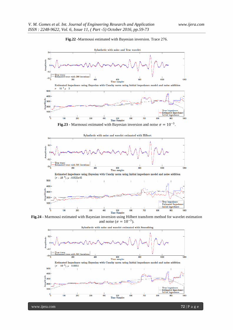
By observing the influence of noise, Fig.23,

Fig.24 and Fig.25 prove the method as more

efficient than the previous to deal with these

situations, even when using estimated wavelets. A

characteristic effect of noise are the artifacts with

oscillatory behavior in the calculated impedance,

easily noticeable in the last two above-mentioned

figures what however, does not prevent the

identification of the main interfaces. Finally it is

reiterated that the good performance of the method is

highly dependent on the above mentioned

parameters so that, good results can only be

achieved through a good estimate of these.Regarding

the performance tests with estimated wavelets, again

this method outperforms the Narrow Band,

achieving good results for the two estimation

techniques. In tests with the noise, however, the

presence of the artifacts discussed is significant,

especially when using wavelets estimated by Hilbert

transform method (Fig.24). By observing the results,

once again the Smooth appeared as the best

alternative, although in the tests discrepancies were

not as evident, showing that the Bayesian can solve

for uncertainties associated with the estimation of

the wavelet. Fig.26 and Fig.27 illustrate the

differences for results with both estimated wavelets.

As a final discussion about this method, the

artifacts in Fig. Fig.21 will be treated. They emerge

as a consequence of numerical instability during the

Conjugate Gradient optimization. As the inversion is

performed trace by trace, situations where the

method cannot converge well or when errors

associated with numerical approximation appear

might happen, justifying the artifacts in a few traces.

Nonetheless, the Conjugate Gradient method

minimizes the misfit with a step size per iteration,

the search for this step size is referred as line search

and was implemented here in a somehow empirical

way, where from an initial value the next was found

through fitting a polynomial between the previous

and values closer to it. Therefore the selected step

size could go over the global minimum hence

increasing the error and leading to the discussed

discontinuities.Comparison of the above results

show that Bayesian inversion has guaranteed less

estimation errors, proving superior to Narrow-band

for all tests. However, it is necessary to mention that

its computational cost is higher, in some cases

requiring more than 100 iterations for convergence

to an acceptable result. In any case, its sensitivity to

the uncertainties introduced by noise and estimated

wavelet is smaller, what can justify its choice over

the Narrow-band.

IV. CONCLUSION

Arising from the need to obtain estimates of

the parameters associated with subsurface geology

mainly with the purpose of exploration, geophysical

methods have increasingly gained space once it is an

indirect way and therefore more economical. In the

case of the seismic method, probably the most

popular, information on acoustic properties can be

obtained using seismic inversion algorithms, among

which two were discussed here, Narrow band and

Bayesian.The proposed methodology aimed to test

the sensitivity of the inversion methods considering




estimated wavelets and noise. Comparison of the

wavelet estimation methods showed that Smooth

produces better results. However, the amplitude

spectrum of the estimated wavelets showed that both

can solve the problem. Phase spectrum analysis

indicates otherwise, so that even after APC phase

correction the spectrum was not well approximated.

Techniques that are able to produce better estimates

to the phase spectrum would obtain in this way,

superior results.For inversion, the tests indicated

Bayesian as the most efficient once it converged to

the real model in all tests, even in the most complex

situation with wavelet estimated and noise, though

artifacts appeared in the inverted data. Anyway this

method produces good estimates of the impedance

model, delimiting all the interfaces and solving the

uncertainties related with both the noise and an

estimated wavelet. Summarizing, through the tests

carried out, the inversions methods performed well

under a low noise level situation (which can be

accomplished through robust pre-conditioning

techniques) and showed uncertainty in the wavelet

estimation can affect drastically inversion results.

Moreover, even though no well information was

input to the experiments, statistical wavelets

provided good results. Finally It can also be inferred

that by using a consistent low frequency model these

wavelets are valid though a comparison between

them and deterministic wavelets in the seismic

inversion context should be performed to confirm

this.

ACKNOWLEDGEMENTS

The authors thank Petrobras for the

financial support to the infrastructure of the GISIS

(Group of Seismic Inversion and Imaging) Research

Group. We are grateful to the members of the Group

for the comments and discussions. We also thankful

to the Department of Geology and Geophysics of

Universidade Federal Fluminense for allowing this

work to be completed.

REFERENCES

[1]. B.H. Russell, Introduction to seismic

inversion methods (Society of Exploration

Geophysicists, 1988).

[2]. D.A. Cooke, W.A. Schneider, Generalized

linear inversion of reflection seismic data,

Geophysics, 48(6), 1983, 665-676.

[3]. T.J. Campbell, F.W.B. Richards, R.L.

Silva, G. Wach, L. Eliuk, Interpretation of

the Penobscot 3D seismic volume using

constrained sparse spike inversion, Sable

sub-Basin, offshore Nova Scotia, Marine

and Petroleum Geology, 68(Part A), 2015,

73-93.

[4]. J.J. Kormylo, J. Mendel, Maximum

likelihood detection and estimation of

bernoulli-gaussian processes, Information

Theory, IEEE Transactions on, 28(3), 1982,

482-488.

[5]. C. Chi, J. Goutsias, J. Mendel, A fast

maximum-likelihood estimation and

detection algorithm for bernoulli-gaussian

processes, Acoustics, Speech, and Signal

Processing , IEEE International

Conference on ICASSP'85, 10, 1985, 1297-

1300.

[6]. B. Ursin, O. Holberg, Maximum-likelihood

estimation of seismic impulse responses,

Geophysical Prospecting, 33(2), 1985, 233-

251.

[7]. D. Oldenburg, T. Scheuer, S. Levy,

Recovery of the acoustic impedance from

reflection seismograms, Geophysics,

48(10), 1983, 1318-1337.

[8]. M.D. Sacchi, Reweighting strategies in

seismic deconvolution, Geophysical

Journal International, 129(3), 1997, 651-

656.

[9]. Y. Wang, Seismic impedance inversion

using l1-norm regularization and gradient

descent methods, Journal of Inverse and

Ill-posed Problems, 18(7), 2011, 823-838.

[10]. T.J. Ulrych, M.D. Sacchi, Information-

based inversion and processing with

applications, 36 (Elsevier, 2005).

[11]. O. Osman, E. Robinson, Seismic source

signature estimation and measurement,

Geophysics Reprint Series (Society of

Exploration Geophysicists, 1996).

[12]. E.A. Robinson, Predictive decomposition of

time series with applications to seismic

exploration, PhD thesis, Massachusetts

Institute of Technology, Cambridge, MA,

1954.

[13]. T. Ulrych, Application of

homomorphicdeconvolution to seismology,

Geophysics, 36(4), 1971, 650-660.

[14]. A.V. Oppenheim, Superposition in a class

of nonlinear systems, Technical Report,

DTIC Document, 1965.

[15]. D.R. Velis, T.J. Ulrych, Simulated

annealing wavelet estimation via fourth-

order cumulant matching, Geophysics,

61(6), 1996, 1939-1948.

[16]. J. Zheng, S. ping Peng, M. chu Liu, Z.

Liang, A novel seismic wavelet estimation

method, Journal of Applied Geophysics,

90(0), 2013, 92-92.

[17]. B. Yi, G. Lee, H.J. Kim, H.T. Jou, D. Yoo,

B. Ryu, K. Lee, Comparison of wavelet

estimation methods, Geosciences Journal,

17(1), 2013, 55-63.

[18]. Z. Wang, B. Zhang, J. Gao, The residual

phase estimation of a seismic wavelet using




a rényi divergence-based criterion, Journal

of Applied Geophysics, 106(0), 2014, 96-

105.

[19]. S.A.M. Oliveira, W.M. Lupinacci, L1 norm

inversion method for deconvolution in

attenuating media, Geophysical

Prospecting, 61(4), 2013, 771-777.

[20]. S. Levy, D. Oldenburg, Automatic phase

correction of common-midpoint stacked

data, Geophysics, 52(1), 1987, 51-59.

[21]. O. Yilmaz, Seismic data analysis:

processing, inversion and interpretation of

seismic data (Society of Exploration

Geophysicists, 2nd edition, 2001).

[22]. E.A. Robinson, S. Treitel, Geophysical

signal analysis (Society of Exploration

Geophysicists, 2000).

[23]. L.R. Lines, T.J. Ulrych, The old and the

new in seismic deconvolution and wavelet

estimation, Geophysical Prospecting, 25(3),

1977, 512-540.

[24]. N. Wiener, Extrapolation, interpolation,

and smoothing of stationary time series:

with engineering applications (The MIT

Press, 1966).

Fig.21 -Marmousi estimated with Bayesian inversion for full seismogram and 1000 iterations per trace.




Fig.22 -Marmousi estimated with Bayesian inversion. Trace 276.

Fig.23 - Marmousi estimated with Bayesian inversion and noise 𝜎 = 10−3.

Fig.24 - Marmousi estimated with Bayesian inversion using Hilbert transform method for wavelet estimation

and noise (𝜎 = 10−3).




Fig.25 - Marmousi estimated with Bayesian inversion using Smooth spectra method for wavelet estimation and

noise (𝜎 = 10−3).

Fig.26 - Marmousi estimated with Bayesian inversion using Hilbert transform method for wavelet estimation

without noise.

Fig.27 -Marmousi estimated with Bayesian inversion using Smooth spectra method for wavelet estimation and

without noise.

Evaluation of the Sensitivity of Seismic Inversion … · V. M. Gomes et al. Int. Journal of...

Documents

Transcript of Evaluation of the Sensitivity of Seismic Inversion … · V. M. Gomes et al. Int. Journal of...