Evaluation of the impacts of soil and water conservation practices on

ecosystem services in Sasumua watershed,

Kenya, using SWAT model

Hosea Munge Mwangi

A thesis submitted in partial fulfillment for the degree of Master of

Science in Environmental Engineering and Management in the Jomo

Kenyatta University of Agriculture and Technology

2011

DECLARATION

This thesis is my original work and has not been presented for a degree in any other

University.

Signature________________________ Date_______________________

Hosea Munge Mwangi

This thesis has been submitted for examination with our approval as University

Supervisors

1. Signature________________________ Date_______________________

Prof. John M. Gathenya

JKUAT, KENYA

2. Signature________________________ Date_________________________

Prof. Bancy M. Mati

JKUAT, KENYA

i

DEDICATION

I dedicate this work to mum (Margaret), dad (Onesmus) and my siblings (Irene, Susan,

Beth, Obadiah, Gilson and Julius).

ii

ACKNOWLEDGEMENT

First of all I wish to thank my dear parents, brothers and sisters for their continued

support and patience throughout my studies. I deeply thank my wife Grace, whom we

got married in the final phase of writing this thesis and whose support and prayers I

greatly value. Not to forget my cousin’s family (Hannah and Samuel) who hosted me for

sometime, supported and encouraged me a lot during my higher education. To my

extended family and friends who supported me financially, in prayers or through

encouragement I say thank you.

I would like to pass my sincere gratitude to my supervisors Prof. John Gathenya and

Prof. Bancy Mati for their guidance throughout the research. I would also wish to thank

Mr. John Mwangi for the support accorded to me in terms of input data collection

especially in the first stages of the study. Special thanks to Sanjeeb Bhattarai, a Nepali

MSc. student at Bangor University United Kingdom, whom we worked together during

the field visits.

I would also wish to recognize Prof. George Ndegwa the university coordinator for

CIMO NSS programme in JKUAT through whom I got a scholarship to Lappeenranta

University of Technology (LUT), Finland from where I did most of the work. I

appreciate Prof. Andrezej Kraslawski from chemical technology department, LUT and

the CIMO NSS coordinator at LUT who took his time to read my work and ensuring my

iii

comfortable stay at Lappeenranta. My appreciation also goes to my colleagues and

classmates Joy N. Riungu, Matolo Nyamai and Wamuyu Gathinji for their

encouragements.

I wish to acknowledge the financial support I received from Jomo Kenyatta University

of Agriculture and Technology and the Macaulay Land Use Research Institute, UK.

Through the Building Ecosystem Services Research Capacity for Semi-Arid Africa

(BESSA) project.

Above all, may the Almighty God receive glory and honour for the gift of good health

and sufficient grace during the study.

iv

TABLE OF CONTENTS

DECLARATION...............................................................................................................i

DEDICATION................................................................................................................. ii

ACKNOWLEDGEMENT............................................................................................. iii

TABLE OF CONTENTS.................................................................................................v

LIST OF TABLES ..........................................................................................................ix

LIST OF FIGURES .........................................................................................................x

LIST OF APPENDICES ................................................................................................xi

ABBREVIATIONS AND ACRONYMS..................................................................... xii

ABSTRACT.................................................................................................................. xiii

CHAPTER 1 .....................................................................................................................1

INTRODUCTION............................................................................................................1

1.0 Background ........................................................................................................1

1.1 Problem statement..............................................................................................3

1.2 Justification ........................................................................................................4

1.3 Objectives...........................................................................................................5

1.3.1 Main Objective:.............................................................................................5

1.3.2 Specific objectives: .......................................................................................5

1.4 The Study area....................................................................................................5

1.4.1 Soils...........................................................................................................8

1.4.2 Land use/land cover ..................................................................................9

v

1.4.3 Rainfall and temperature .........................................................................12

CHAPTER 2 ...................................................................................................................13

LITERATURE REVIEW..............................................................................................13

2.1 Ecosystem services and livelihoods .................................................................13

2.2 Soil erosion ......................................................................................................17

2.2.1 Universal soil Loss Equation (USLE)......................................................18

2.3 Soil and water conservation practices ..............................................................21

2.4 Agronomic and Vegetative Conservation measures ........................................23

2.4.1 Contour farming .......................................................................................23

2.4.2 Vegetative filter strips ..............................................................................25

2.5 Structural conservation Practices ....................................................................30

2.5.1 Terraces ....................................................................................................30

2.5.2 Grassed waterway ....................................................................................33

2.6 Soil and water conservation in Kenya..............................................................35

2.7 Hydrological modeling ....................................................................................36

2.8 SWAT overview: Sediment and hydrology theory..........................................38

2.8.1 Climatic inputs for SWAT .......................................................................39

2.8.2 Calibration of SWAT model ...................................................................40

2.8.3 Hydrology in SWAT................................................................................41

CHAPTER 3 ...................................................................................................................52

MATERIALS AND METHODS ..................................................................................52

3.1 Data collection .................................................................................................52

vi

3.1.1 DEM, Land use/Land cover and Soil Data ..............................................52

3.1.2 Climatic data ............................................................................................53

3.1.3 Reservoir levels data ................................................................................54

3.1.4 Site visits and farmer interviews..............................................................54

3.2 Model setup for base scenario..........................................................................56

3.3 Parameter Sensitivity analysis .........................................................................58

3.4 Model Calibration ............................................................................................59

3.5 Model Validation .............................................................................................60

3.6 Simulation of soil and water conservation Practices........................................61

3.6.1 Vegetative Filter strips .............................................................................61

3.6.2 Contour farming ......................................................................................62

3.6.3 Bench terraces .........................................................................................64

3.6.4 Grassed waterway ...................................................................................66

3.6.5 Additional management scenarios ..........................................................66

CHAPTER 4 ...................................................................................................................68

RESULTS AND DISCUSSION ....................................................................................68

4.1 Farmer interviews ............................................................................................68

4.1.1 Land use/land cover .................................................................................68

4.1.2 Soil conservation practices in Sasumua ...................................................70

4.2 Parameter Sensitivity analysis .........................................................................72

4.3 Model Calibration ............................................................................................76

4.4 Model Validation .............................................................................................78

vii

4.5 simulation of soil and water conservation practices ........................................79

4.5.1 Vegetative filter strips .............................................................................79

4.5.2 Contour Farming ......................................................................................84

4.5.3 Contour farming and filter strips..............................................................90

4.5.4 Terracing ..................................................................................................91

4.5.5 Grassed waterway ....................................................................................94

4.5.6 Additional management scenarios ...........................................................98

CHAPTER 5 .................................................................................................................101

CONCLUSIONS AND RECOMMEDATIONS........................................................101

5.1 Conclusions....................................................................................................101

5.2 Recommendations ..........................................................................................103

REFERENCES.............................................................................................................106

APPENDICES ..............................................................................................................119

viii

LIST OF TABLES

Table 1: Percentage land use/land cover ....................................................................11

Table 2: Typical y values for determining terrace intervals.......................................33

Table 3: Management operations modelled for the agricultural land ........................56

Table 4: USLE-P values for contour farming, strip cropping and terracing ..............63

Table 5: Top most sensitive parameters for stream flow and sediment and the range

of values used for base simulation ..............................................................74

Table 6: Mean simulated sediment yield for contour farming, contour farming and 5

m filter strip width and terracing.................................................................84

Table 7: Water balance for base simulation and for simulation of contour farming..89

Table 8: Water balance for the simulation of bench terraces in Sasumua watershed 93

Table 9: Simulated sediment yield and stream flow reduction with and without

grassed waterway. .......................................................................................95

Table 10: Sediment loading and water balance for good (CN-6) and poor (CN+6)

management cases.......................................................................................99

ix

LIST OF FIGURES

Figure 1.1: Sasumua watershed ....................................................................................7

Figure 1.2: Soils in Sasumua watershed.......................................................................9

Figure 1.4: Monthly rainfall distribution for Sasumua dam station ...........................12

Figure 2.1: Ecosystem services and their link to human well being ..........................15

Figure 2.2: Grass filter strip in Sasumua ....................................................................27

Figure 2.3: Prism and wedge storages in a reach segment .........................................44

Figure 2.4: Relationship between slope and slope length ..........................................50

Figure 3.1: Interview with one of the famers .............................................................55

Figure 3.2: Sub-basins as simulated in SWAT model................................................57

Figure 3.3: Sub-basins simulated with terraces ..........................................................65

Figure 4.1:. Percentage Land use.................................................................................70

Figure 4.2: Napier grass strip in one of the farms in Sasumua...................................71

Figure 4.3: Highly turbid water flowing to Sasumua Reservoir.................................72

Figure 4.4. ‘Measured’ and simulated stream flows ..................................................78

Figure 4.5: Measured and simulated stream flow......................................................79

Figure 4.6: Total decrease and percent reduction in sediment yield .........................80

Figure 4.7 (a): sediment yield for base simulation...................................................87

Figure 4.7 (b): sediment yield after implementation of contour farming.................87

Figure 4.8: Effect of contour farming and Bench terraces on water balance .............94

x

LIST OF APPENDICES

Appendix 1: Slope length of sub-basins……………………………………………119

Appendix 2: Questionnaire…………………………………………………………120

Appendix 3: Sediment yield for base simulation…………………………………...123

xi

ABBREVIATIONS AND ACRONYMS

DEM Digital Elevation model

GIS Geographical Information Systems

GWW Grassed Waterway

HRU Hydrologic Response Unit

ICRAF World Agroforestry Center

MA Millennium Ecosystem Assessment

MUSLE Modified Universal Soil Loss Equation

NRCS Natural Resources Conservation Service

NSE Nash-Sutcliffe Efficiency

NCWSC Nairobi City Water and Sewerage Company

PES Payment of Ecosystem Services

PRESA Pro-poor Reward for Environmental Services in Africa

RUSLE Revised Universal Soil Loss Equation

USLE Universal Soil Loss Equation

VFSMOD Vegetative Filter Strip Model

SWAT Soil and Water Assessment Tool

USDA United States Department of Agriculture

CN Curve Number

USLE_P Universal Soil Loss Equation practice factor

xii

ABSTRACT

Degradation of agricultural watersheds reduces the capacity of agro-ecosystems to

produce Ecosystem Services such as improving water quality and flood mitigation.

Conservation of degraded watersheds can abate water pollution and regulate stream

flows by reducing flash floods and increasing base flow as a result of enhanced

infiltration. The objective of this study was to evaluate the effect of soil and water

conservation practices on hydrology and water quality in Sasumua watershed, Kenya

using Soil and Water Assessment Tool (SWAT) model. Vegetative filter strips, contour

farming, bench terraces and grassed waterways were the conservation measures

assessed. They were represented by adjusting relevant parameters in the model and the

resulting effect on sediment yield and stream flow assessed. The width of the filter strip

was adjusted to simulate vegetative filter strip, USLE-P and CN were adjusted to

simulate contour farming and terraces were simulated by adjusting CN, USLE-P and

slope length appropriately. Grassed waterways were simulating by adjusting CH_N2,

CH_EROD and CH_COV parameters in the model. Two additional simulations were

also done to compare alternative management scenarios.

It was found that the reduction in sediment yield increased with increase in width of the

filter strip but the increase was logarithmic. A 5-meter width was predicted to reduce

sediment loading by 38% when simulated in the agricultural part of the sub-watershed.

Simulation of contour farming reduced sediment yield for entire Sasumua sub-watershed

xiii

(67.44 Km2), from the base simulation value of 32,620 tyr-1 to 16,600 tyr-1 representing

a 49% decrease. Contour farming decreased the surface runoff by 16% from 193 mm for

base simulation to 162 mm and increased base flow from 304 mm to 327 mm an

increase of about 7.5%. A combination of 5 meter vegetative filter strip and contour

farming were predicted to result in a reduction of 73% of sediment yield. The sediment

yield reduced to 8720 tyr-1 from the base simulation value 32,620 tyr-1. Simulation of

bench terraces reduced sediment load to 4930 tyr-1. This represents 85% decrease. The

surface runoff decreased by 22% from 193mm to 151 mm while base flow increased

from 304mm to 335mm which is an increase of 10%. Both the contour farming and

terraces resulted in only a slight change in total water yield. Grassed waterway simulated

for some drainage ditches in the watershed reduced sediment load from 20,600 tyr-1 to

12,200 tyr-1 at the outlet downstream of the drainage channels that represents a reduction

of 41%. For the entire sub-watershed, grassed waterway reduced the sediment yield

from 32,600 tyr-1 to 25,000 tyr-1 which represents a 23.5% decrease. A management

scenario that simulated less intensive cultivation in agricultural lands and proper

managed grazing in grasslands resulted in a reduction of 34% sediment yield. The

sediment yield reduced from 32,620 tyr-1 to 21,430 tyr-1. The surface runoff reduced by

28% from 278 mm to 138 mm and the base flow increased by about 14% from 304 mm

to 346 mm for this scenario. A management scenario that simulated more intensive

cultivation in agricultural lands and overgrazing in grasslands was found to have a

53.6% increase in sediment yield, 44% increase in surface runoff and about 10%

decrease in base flow. The sediment yield for this scenario increased from 32,620 tyr-1 to

xiv

50,100 tyr-1 while the surface runoff increased to 278 mm from 193 mm and the base

flow reduced from 304 mm to 272 mm.

Thus all the conservation practices investigated were found to have a positive impact in

enhancing the ecosystem services. Soil erosion ‘hotspots’ which should be prioritized in

conservation were identified. Bench terraces were found to be the most effective. It is

recommended that bench terraces should be constructed in the watershed especially on

the soil erosion ‘hotspots’. For the farmers who may not be able to construct the bench

terraces due to cost, grass strips should be planted as they would evolve to bench

terraces with time. Grassed waterways should also be constructed on the drainage

channels that feed Mingotio stream. The Nairobi City Water and Sewerage Company

and Water Resources Management Authority should rehabilitate the gauge stations and

be collecting stream flow and water quality data. This would be important for better

planning and would be of more help in future research work. Further research on the

willingness of the farmers to accept to engage in soil and water conservation should be

done. The cost of implementing the conservation practices should also be carried out.

xv

CHAPTER 1

INTRODUCTION

1.0 Background

Ecosystems produce services which are important and beneficial to human beings.

Ecosystem services are the benefits the ecosystems provide for human wellbeing.

(Millennium Ecosystem Assessment, MA, 2003). Ecosystem services range from

provision of products such as food, timber, fuel wood and fresh water to other non

tangible benefits such as flood regulation, water purification and aesthetics among

others. Human livelihoods form an integral part of the ecosystem and ecosystem services

are linked to the sustainability of human life (Millennium Ecosystem Services, MA,

2003). Indeed life on earth depends of sustainable flow of these services. Ecosystems are

complex in structure, composition and in the interactions of their components.

Sustainable management calls for a thorough understanding of the effects of over

exploitation of natural resources, otherwise the exploitation may lead to adverse

consequences (Chi, 2000). Therefore, proper management of watersheds is required for

continued enjoyment of the ecosystem services.

Sasumua watershed located in the central highlands of Kenya is a key ecosystem to the

Kenyan economy. Some of the ecosystem goods and services produced by Sasumua

watershed include food, fuel wood, timber, freshwater, water flow regulation and water

1

purification. The watershed has a reservoir (Sasumua) which supplies about a fifth of the

water consumed in Nairobi. The watershed is partly agricultural and its proximity to

Nairobi makes the place it a major supplier of agricultural produces such as potatoes,

cabbages and milk to the city.

In the last 10 years more people have settled in the area because of the favourable

climate. Based on demographic data of Njabini location, where Saumua watershed is

located, the population growth rate was 3.8% per year (Mireri, 2009). Based on the 1999

population census and projections indicates that in 2008, population of the location was

41,029 people having risen from 30,486 in 1999 (Mireri, 2009). This increase in

population has caused an increase in demand in natural resources including land and

water (Mireri, 2009).

Human activities in Sasumua watershed are causing changes on the ecosystem and

limiting its capability to sustainably produce these services and goods. Intense

cultivation and overgrazing in some parts of the watershed has caused land degradation.

Research done in the area revealed that overgrazing in some parts of the watershed has

reduced the water infiltration rates of water increasing the overland flow. The increased

surface runoff greatly increases soil erosion risk, and leading to further degradation

(Vagen, 2009).

2

1.1 Problem statement

The pressure on the natural resources namely land and water in Sasumua has increased

in the recent past due increase in population (Mireri, 2009). Soil erosion in the

watershed has increased due to intense cultivation of land and high runoff which results

from low infiltration rates in the degraded land (Vagen, 2009). The soil eroded from the

watershed is washed to the streams and eventually to the Sasumua reservoir (Gathenya

et al., 2009). Water treatment process at the reservoir includes removal of sediments

some of which result from soil erosion. Accelerated soil erosion in the watershed result

in high treatment cost of the water from the reservoir.

Water resources are also dwindling against the increasing demand (Mireri, 2009). The

Sasumua dam which supplies 20% of water to Nairobi experiences shortage of water in

dry seasons of the year and this has been partly blamed on the anthropogenic activities in

the watershed (Mireri, 2009). With reduced infiltration of water in the watershed, high

flash floods occur whenever it rains. The increased runoff fills the reservoir and the most

goes over the spillway. However, less water infiltrates to recharge the aquifer and thus

low flows characterize the streams in the watershed immediately after the rains as a

result of reduced base flows (Vorosmarty et al., 2003).

Therefore, the main problems in Sasumua watershed addressed in this study are the high

rate of soil erosion from the agricultural part of the watershed and declining water levels

in the Sasumua dam. Thus the intention of this study was to simulate the effect of soil

3

and water conservation practices on sediment yield and hydrology in Sasumua

Watershed using Soil and Water Assessment Tool (SWAT) model.

1.2 Justification

Previous studies by Gathenya et al. (2009) and Vagen, (2009), have recommended the

implementation of soil and water conservation measures in the watershed. The

implementation of which will address the issue of soil erosion and regulation of stream

flows to the Sasumua reservoir.

There are many soil and water practices that can reduce soil erosion and regulate the

water flows by increasing the infiltration of water to the ground. Such practices include

terraces, contour farming, riparian buffer strips, contour grass strips, and hedges

(Biamah et al., 1997). Implementation of any of these soil and water conservation

practices in the Sasumua watershed would solve the problem of soil erosion and low

levels of water in the reservoir to different degrees. Thus it is important to study the

level to which each of these measures would address the problem of soil erosion on the

land, sedimentation in the rivers and the Sasumua dam, and regulation of flows in the

watershed. To do these, a watershed model was used to simulate scenarios of sediment

yield and hydrology with different agricultural practices. For these reasons this study

used a physically based watershed hydrological model, SWAT to simulate the effect of

4

different agricultural conservation measures to water and sediment yield of the Sasumua

watershed.

1.3 Objectives:

1.3.1 Main Objective:

To predict the effect of soil and water conservation practices on water quality and

hydrology of Sasumua watershed.

1.3.2 Specific objectives:

1) To validate the SWAT model for Sasumua watershed

2) To assess the effect of implementing agronomic and vegetative conservation

practices on water and sediment yield in Sasumua watershed

3) To assess the effect of implementing structural conservation practices on water

and sediment yield.

1.4 The Study area

Sasumua watershed on the slopes of Aberdare ranges lies between longitudes 36.58°E

and 36.68°E and latitudes 0.65°S and 0.78°S and has an altitude of between 2200m and

3850m (Figure 1.1) It is located in South Kinangop District of Central Province and in

Nyandarua County. Sasumua reservoir receives water from three sub-watersheds

(Figure 1.1). Sasumua sub-watershed (67.44 km2) which is seasonal and provides water

5

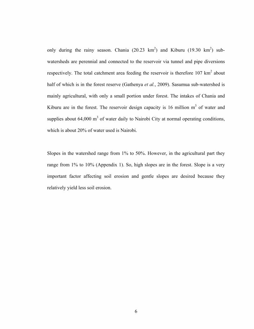
only during the rainy season. Chania (20.23 km2) and Kiburu (19.30 km2) sub-

watersheds are perennial and connected to the reservoir via tunnel and pipe diversions

respectively. The total catchment area feeding the reservoir is therefore 107 km2 about

half of which is in the forest reserve (Gathenya et al., 2009). Sasumua sub-watershed is

mainly agricultural, with only a small portion under forest. The intakes of Chania and

Kiburu are in the forest. The reservoir design capacity is 16 million m3 of water and

supplies about 64,000 m3 of water daily to Nairobi City at normal operating conditions,

which is about 20% of water used is Nairobi.

Slopes in the watershed range from 1% to 50%. However, in the agricultural part they

range from 1% to 10% (Appendix 1). So, high slopes are in the forest. Slope is a very

important factor affecting soil erosion and gentle slopes are desired because they

relatively yield less soil erosion.

6

#*

#*!(!( !(!(Sasumua

Others

Chania

Kiburu

36°42'0"E

36°42'0"E

36°36'30"E

36°36'30"E

0°37'30"S 0°37'30"S

0°43'0"S 0°43'0"S

0°48'30"S 0°48'30"SLegend!( Intake

#* Weather station

Stream

Chania tunnel

Kiburu pipe

Sasumua Reservoir

Sub-watershed boudary

0 1 2 3 4Kilometers ±

Figure 1.1: Sasumua watershed showing sub-watersheds (inset- location of Sasumua in

map of Kenya)

7

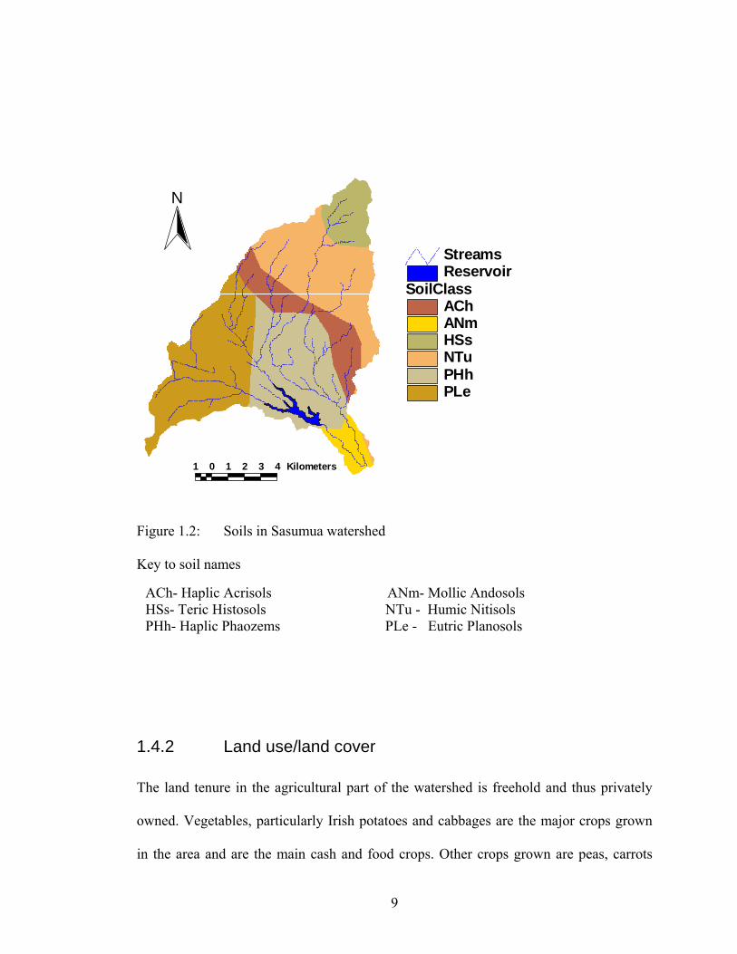
1.4.1 Soils

The soils in Sasumua from the high mountainous Northeastern end are Histosols,

Nitisols, Acrisols, Phaeozems, and Planosols on the lower Southwestern plateau area

(Figure 1.2). Andosols are also present downstream of the dam (Vagen, 2009). The main

agricultural part of Sasumua sub-watershed is composed mainly of Planosols,

characterized by a weakly structured surface horizon over an albic horizon with `stagnic

soil properties'. The texture of these horizons is coarse and there is an abrupt textural

change to the underlying deeper soil layers. The finer textured subsurface soil may show

signs of clay illuviation. It is only slowly permeable to water. Periodic stagnation of

water directly above the denser subsurface soil produced typical stagnic soil properties

in the bleached, eluvial horizon. (FAO, 2001)

8

1 0 1 2 3 4 Kilometers

SoilClassAChANmHSsNTuPHhPLe

ReservoirStreams

N

Figure 1.2: Soils in Sasumua watershed

Key to soil names

ACh- Haplic Acrisols ANm- Mollic Andosols HSs- Teric Histosols NTu - Humic Nitisols PHh- Haplic Phaozems PLe - Eutric Planosols

1.4.2 Land use/land cover

The land tenure in the agricultural part of the watershed is freehold and thus privately

owned. Vegetables, particularly Irish potatoes and cabbages are the major crops grown

in the area and are the main cash and food crops. Other crops grown are peas, carrots

9

and kales. In the recent past, few farmers have also turned to growing cut flowers for

export. The agricultural area borders a forest reserve (Aberdare forest) to the North of

the watershed. The farmers also keep livestock and some portions of the farms are

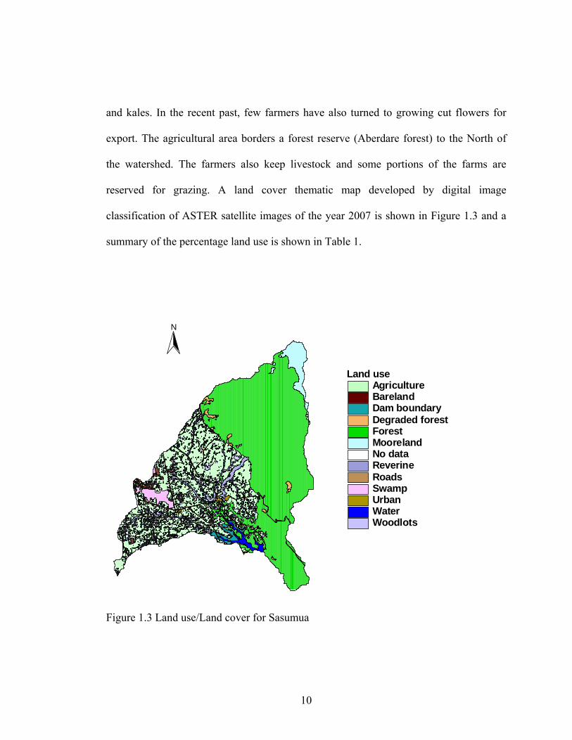
reserved for grazing. A land cover thematic map developed by digital image

classification of ASTER satellite images of the year 2007 is shown in Figure 1.3 and a

summary of the percentage land use is shown in Table 1.

Land useAgricultureBarelandDam boundaryDegraded forestForestMoorelandNo dataReverineRoadsSwampUrbanWaterWoodlots

N

Figure 1.3 Land use/Land cover for Sasumua

10

The same thematic map was used as the input in the SWAT model. Forest and

agriculture cover the biggest area of the watershed. Also to note is the wetland (swamp)

which the farmers are slowly opening for cultivation.

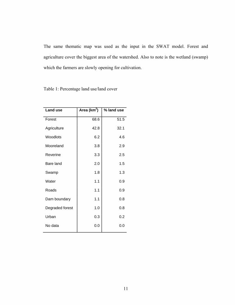
Table 1: Percentage land use/land cover

Land use Area (km2) % land use

Forest 68.6 51.5

Agriculture 42.8 32.1

Woodlots 6.2 4.6

Mooreland 3.8 2.9

Reverine 3.3 2.5

Bare land 2.0 1.5

Swamp 1.8 1.3

Water 1.1 0.9

Roads 1.1 0.9

Dam boundary 1.1 0.8

Degraded forest 1.0 0.8

Urban 0.3 0.2

No data 0.0 0.0

11

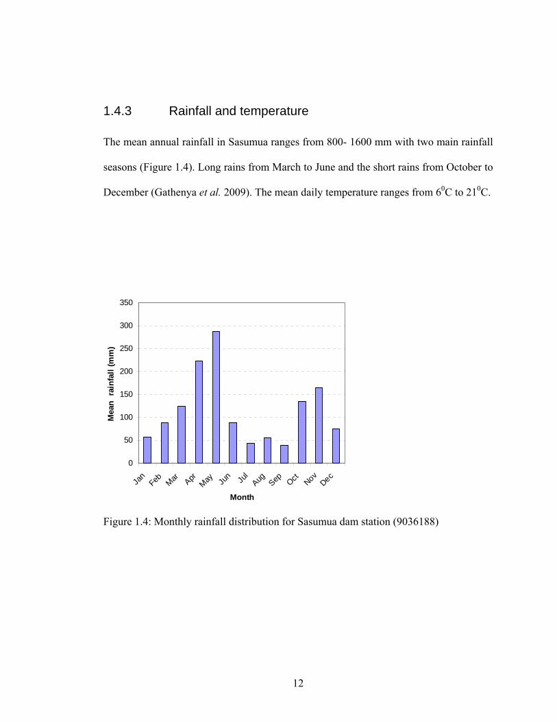
1.4.3 Rainfall and temperature

The mean annual rainfall in Sasumua ranges from 800- 1600 mm with two main rainfall

seasons (Figure 1.4). Long rains from March to June and the short rains from October to

December (Gathenya et al. 2009). The mean daily temperature ranges from 60C to 210C.

0

50

100

150

200

250

300

350

Jan

Feb Mar AprMay Ju

n Jul

Aug Sep Oct NovDec

Month

Mea

n ra

infa

ll (m

m)

Figure 1.4: Monthly rainfall distribution for Sasumua dam station (9036188)

12

CHAPTER 2

LITERATURE REVIEW

2.1 Ecosystem services and livelihoods

In general, ecosystems are dynamic complexes of plant, animal and micro-organism

communities and their nonliving environment interacting as functional units (MA,

2003). The Millennium Ecosystem Assessment (MA, 2003) defines ecosystem services

as the benefits ecosystems provide for human well-being. Based on this, four main

classes of ecosystem services can be identified. These are the provisioning, regulating,

supporting and cultural services. Provisioning services cover natural resources and

products derived from ecosystems such as food, fuel, fiber, fresh water, and genetic

resources and represent the flow of goods. Regulating or supporting services are the

actual life-support functions ecosystems provide. In other words, they are the benefits

people obtain from the regulation of ecosystem processes, including air quality

maintenance, climate regulation, erosion control, regulation of human diseases, and

water purification and are normally determined by the size and quality (the stock) of the

ecosystem. Cultural services refer to the non-material benefits obtained from ecosystem

services such as spiritual and religious significance and other benefits like recreation and

aesthetic experiences. Supporting services are those that are necessary for the production

of all other ecosystem services, such as primary production, production of oxygen, and

soil formation (Iftikhar et al., 2007; MA, 2003).

13

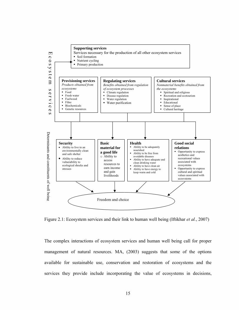
Ecosystems are linked to people and they offer benefits to the human-beings and

especially the poor. Figure 2.1 depicts the links between ecosystem services and human

beings. The MA framework assumes that there is a dynamic interaction that exits

between people and other parts of the ecosystems. Changes in the human conditions can

directly or indirectly drive change in the ecosystems and changes in ecosystems can also

cause change in human well-being. Changes in ecosystem services affect human well-

being through impacts on security, the basic material for a good life, health, and social

and cultural relations (MA, 2003). Security can for example be affected by changes in

the provisioning services which would affect the supply of food and other goods. A

community’s food security would be threatened if the ecosystem fails to produce enough

food. Security is also affect by the conflict over the declining resources such as water

and grazing land. Food and clean fresh drinking water are basic commodities for human

livelihood. Therefore there is a strong link between ‘Access to basic material for a good

life’ and provisioning services such as food and fiber production and regulating services,

including water purification. Health is strongly linked to both provisioning services such

as food production and regulating services, including those that influence the

distribution of disease-transmitting insects and of irritants and pathogens in water and

air. Health is also linked to cultural services through recreational and spiritual benefits.

Social relations are affected by changes to cultural services, which affect the quality of

human experience. Freedom of choice and action is based on the existence of the other

components of well-being and are thus influenced by changes in provisioning,

regulating, or cultural services from ecosystems.

14

Supporting services Services necessary for the production of all other ecosystem services Soil formation Nutrient cycling Primary production

Provisioning services Products obtained from ecosystems Food Fresh water Fuelwood Fibre Biochemicals Genetic resources

Security • Ability to live in an

environmentally clean and safe shelter

• Ability to reduce vulnerability to ecological shocks and stresses

Basic material for a good life o Ability to

access resources to earn income and gain livelihoods

Health Ability to be adequately

nourished Ability to be free from

avoidable diseases Ability to have adequate and

clean drinking water Ability to have clean air Ability to have energy to

keep warm and cold

Good social relations Opportunity to express

aesthetics and recreational values associated with ecosystems

Opportunity to express cultural and spiritual values associated with ecosystems

Freedom and choice

Regulating services Benefits obtained from regulation of ecosystem processes Climate regulation Disease regulation Water regulation Water purification

Cultural services Nonmaterial benefits obtained from the ecosystems

Spiritual and religious Recreation and ecotourism Inspirational Educational Sense of place Cultural heritage

Ec

osy

stem

serv

ice

sD

eterminants and constituents of w

ell being

Figure 2.1: Ecosystem services and their link to human well being (Iftikhar et al., 2007)

The complex interactions of ecosystem services and human well being call for proper

management of natural resources. MA, (2003) suggests that some of the options

available for sustainable use, conservation and restoration of ecosystems and the

services they provide include incorporating the value of ecosystems in decisions,

15

channeling diffuse ecosystem benefits to decision-makers with focused local interests,

creating markets and property rights, educating and dispersing knowledge, and investing

to improve ecosystems and the services they provide. Decision making is thus a key

point of intervention in proper management of natural resources. Technical input in the

decision making process is an important element because it offers various approaches

including tools that will aid in analyzing the management options available as well as

the cost benefit analyses. Computer modeling simulation is one approach that can and

has been used in evaluating management options by or for decision makers. The

assessment would for example help understand the spatial distribution of ecosystem

services and where tradeoffs and synergies among ecosystem services exist and come up

with intervention measures suitable at different location of watersheds. Swallow et al.

(2009), for example, assessed the spatial distribution of provisioning and regulating

ecosystem services in Lake Victoria in Kenya covering Nyando and Yala River basins.

Agricultural production and reduction in sediment yield represented the provisioning

and the regulating ecosystem services they studied respectively. They used GIS to

spatially overlay sediment yield output data from SWAT analysis and value of

agricultural production at a scale of SWAT generated sub-basins. They were able to

spatially show the locations that have tradeoffs and those that have synergies between

agricultural production and sediment yield.

16

2.2 Soil erosion

Soil erosion can either be caused by wind (wind erosion) or water referred as water

erosion. Water erosion can be classified as splash, sheet, rill and gully erosion. Splash

erosion occurs when the rain drops hits bare soil surface. Sheet erosion is washing of the

surface soil by water. Rill erosion happens when water concentrates in small channels

and gully erosion happens when the eroded channels get larger (Hudson, 1989). Soil

erosion involves two main processes, the detachment and the transport of soil particles

by the erosive forces of the raindrops and surface flow of water (Neitsch et al., 2005).

Erosion can be defined as a process in which soil particles are detached from within the

surface of a cohesive soil matrix and subsequently moved down slope by one or more

transport agents. Detachment may be caused by raindrop impact on the soil surface or by

shear of the flowing water in case of rainfall erosion. Down slope movement may be

caused by splash erosion, or by interaction between raindrop impact and flow (raindrop-

induced saltation and rolling) or by flow alone (suspension, flow driven saltation and

rolling) (Kinnell, 2010).

Together with soil particles, surface runoff and irrigation return flows carry other

pollutants from the agricultural land. Agricultural chemicals, pathogens (bacteria and

viruses) and nutrients such as phosphorous and nitrogen are some of the examples.

These pollutants if they get into water bodies lower their water quality.

17

2.2.1 Universal soil Loss Equation (USLE)

Universal Soil Loss Equation (USLE) (Wischmeier and Smith, 1978) is the most widely

used equation in estimation of soil loss all over the world (Kinnell, 2010). USLE was

originally developed from over 10,000 plot-years of basic runoff and soil loss data and

data from rainfall simulators applied to field plots in the USA. The main purpose of

developing the equation was to come up with a guide for decision making in the

conservation planning. The equation enables the planners to predict the average soil

erosion rates for different combination of management techniques, cropping system and

control practice for a particular site (Wischmeier and Smith, 1978).

USLE was designed to calculate longtime average soil losses from rill and sheet erosion

under specific conditions. It combines physical and management variables that affect

soil erosion and computes soil loss as a product of six factors that are related to climate,

soil, topography, vegetation and management. It is based on unit plot which is 22.1 m

long and 9% slope and cultivation up and down the slope. The USLE soil loss equation

is;

PCSLKRA = (1)

Where A is the mean annual soil loss (mass/area/year), R is the rainfall-runoff

“erosivity” factor, K is Soil “erodibility” factor, L is the slope length factor, S is the

18

slope steepness factor, C is the cover and management factor and P is the support

practice factor.

Rainfall-Runoff erosivity (R) factor- USLE assumes that when factors other than rainfall

are held constant, storm soil losses from cultivated fields are directly proportional to a

rainstorm parameter, EI, which is a product of total storm energy (E) and the maximum

30 minute rainfall intensity (I30). The relationship however does not have a direct

consideration of runoff and this has been cited as one of its limitation (Kinnell, 2010).

Soil erodibility (K) factor- this is the soil loss rate per erosion index unit for a specific

soil as measured on a unit plot (22.1 m long, 9% slope, in a continuous fallow tilled up

and down the slope). Soil erodibility describes the situation where some soils erode

more easily than others even when all other factors such as topography, rainfall

characteristics, cover and management are the same. The difference is soil erosion is

solely caused by differences soil properties (Wischmeier and Smith, 1978). Thus soil

erodibility is a function of soil physical and chemical properties but silt fraction plays a

major role. The K values can be estimated using soil erodibility nomographs

(Wischmeier and Smith, 1978) since direct field measurements can be very expensive.

In cases where the soil contains less than 70% silt fraction, the mathematical

approximation of K factor (as used in the nomograph) can be expressed as;

1414.1 100)}3(5.2)2(25.3)12()10(1.2{ −− −+−+−= pscomMK (2)

19

Where M is the particle size parameter which is the product of the primary particle size

fractions (percent silt times the quantity 100-minus percent clay), om is the pecent

organic matter, sc is the soil structure class used in the soil classification and p is the

profile permeability class.

Topographic factors (L and S) - slope length is the distance from the origin of the

overland flow to the point where either the slope decreases enough that the deposition

begins or runoff water enters a well-defined channel that may be part of the drainage

network or a constructed channel. The slope length (L) and the slope steepness factor S

are usually combined in the topographic factor LS and are calculated as in equation 14.

Cover and management (C) factor- is the ratio of the long term soil loss from a land with

specific vegetation to the soil loss from clean-tilled continuous fallow on the same soil

cultivated up and down a 22 m long slope with a gradient of 9% (Wischmeier and Smith,

1978; Kinnell, 2010). It measures the combined effect of all the interrelated cover and

management variables.

Support practice (P) factor- is the ratio of soil loss with a specific support practice to the

corresponding loss with up and down slope cultivation. The support practices are

intended to slow runoff water and thus reduce the amount of soil that it can carry.

20

Examples of such support practices include; contour farming, contour-strip cropping and

terrace systems.

Revised USLE (RUSLE) (Renard et al., 1997) is a revision of USLE and uses the USLE

equation with changes on how some of the factors are determined (Kinnell, 2010).

RUSLE1 is a computer program that was developed for implementation of RUSLE

while RUSLE2 provides an approach that takes into account the deposition resulting in

changes in slope gradient on one dimensional hill slopes (Kinnell, 2010). Modified

Universal Soil Loss Equation (MUSLE) (Williams, 1975), is a version of USLE model

that directly considers runoff to estimate sediment yield unlike USLE and RUSLE and

was designed to model erosion at the watershed.

2.3 Soil and water conservation practices

Land owners and managers use various methods to reduce soil erosion and subsequent

pollution of water bodies. The soil and water conservation practices are applied to

agricultural land to abate soil erosion. The practices can be applied at different location

of the agricultural fields and their effectiveness in reducing soil erosion also varies.

World Overview of Conservation Approaches and Technologies (WOCAT) defines Soil

and water conservation as local-level activities that maintain or enhance the productive

capacity of the land in areas affected by, or prone to, degradation. These include

21

activities that prevent or reduce soil erosion, compaction and salinity; conserve or drain

soil water; and maintain or improve soil fertility (Van Lynden and Liniger, 2002).

Various attempts have been made to categorize the soil and water conservation

approaches and technologies. Morgan, (1986), for example, classifies soil conservation

approaches broadly as agronomic measures, mechanical measures and soil management.

Agronomic or biological measures utilize the role of vegetation in helping to minimize

soil erosion. Soil management is concerned with ways of preparing the soil to promote

dense vegetative growth and improve its structures so that it is more resistant to erosion.

Mechanical or physical methods depend upon manipulating the surface topography, e.g.

by construction of terraces to control the movement of water. Hudson (1989), classifies

soil erosion control measures as either mechanical or non-mechanical where in

mechanical measures, mechanical protection works such as earth moving and soil

shaping measures are used. Non-mechanical measures are all practices which influence

and reduce soil erosion by management of growing crops or animals (Hudson, 1989)

WOCAT, a global network of institutions and individuals involved in soil and water

conservation, proposes that the main conservation measures are subdivided as

management, agronomic, vegetative and structural (Liniger et al., 2002). Combinations

are possible and each of these conservation categories is split up into subcategories.

22

2.4 Agronomic and Vegetative Conservation measures

According to WOCAT, agronomic measures are usually associated with annual crops;

are repeated routinely each season or in a rotational sequence; are of short duration and

not permanent; do not lead to changes in slope profile; are normally not zoned; and are

normally independent of slope. Mixed cropping, contour cultivation and mulching are

some of the examples of agronomic measures. Vegetative measures involve the use of

perennial grasses, shrubs or trees; are of long duration; often lead to a change in slope

profile; are often zoned on the contour or at right angles to wind direction and are often

spaced according to slope. Grass strips, hedge rows, windbreaks, alley cropping and

agroforesty systems are some of the examples of vegetative conservation measures

(Liniger et al., 2002; Biamah et al., 1997). Contour farming and vegetative filter strips

are discussed in the next sections.

2.4.1 Contour farming

Contour farming is a form of agriculture where farming activities such as ploughing,

planting cultivating and harvesting are done across the slope rather than up and down the

slope (NRCS, 2006). Crop row ridges built by tilling and planting on the contour create

many small dams. These ridges or dams act as barriers to water flow reducing its

velocity and allowing it more time to infiltrate which reduce surface runoff and soil

erosion. This subsequently reduces sedimentation and siltation of water bodies and thus

improves the water quality. (NRCS, 2006; Quinton and Catt, 2004).

23

Contour farming has been studied well in different parts of the world either through

experimental plots or modeling. Quinton and Catt, (2004) assessed the impacts of

minimal tillage and across-slope cultivations on runoff generation, soil erosion and

yields under arable cropping using the results from 10 years of monitoring water erosion

and runoff at the Woburn Erosion Reference Experiment in Bedfordshire, United

Kingdom. The study reported that cultivation across the slope would reduce the mean

soil loss to 6.4 tons/ha compared to that of up and down slope of 16.5 tons/ha. Although

they acknowledge that the difference was not statistically significant, they recommend

across slope cultivation. This study also found out that the mean event surface runoff

from experimental plots tilled across the slope was about 0.8 mm as compared to 1.32

mm from the experimental plots with up and down cultivation. Gassman et al. (2006)

evaluated the impact of contouring and other BMPs on sediment and nutrient loss in the

upper Maquoketa River watershed in North Eastern Iowa, U.S.A using simulations by

Agricultural Policy Environmental eXtender (APEX) and SWAT models. They found

that contouring reduced sediment loss by an average of 34% from the base simulation

using SWAT over 30 years period of simulation. In another study in Southern Uganda,

Brunner et al. (2008), investigated the influence of different land management methods

on soil erosion by modeling soil loss for individual soil-landscape units on a hillslope

using Water erosion Prediction Project (WEPP) model. They found out that simulated

soil loss for contour farming reduced from 0 to 13% depending on the topography and

soil conditions of the hill slopes as compared to hand hoe tillage practiced by the

24

farmers. Stevens et al. (2009) evaluated the effect of contour cultivation on soil erosion

on experimental field in Leicestershire, England. They found that contour cultivation

reduced surface runoff and sediment yield as compared to up and down cultivation

although the trend was not significantly different. Despite the differences in the

percentage of reduction in surface runoff and sediment yield in these studies or even in

the experimental plots with the same study, they all agree that contour farming reduces

surface runoff and soil erosion if practiced in agricultural watersheds compared to up

and down cultivation methods.

Some of the challenges that have been cited for the adoption of the contour farming are

that on very steep slopes water can accumulate in low points and then break through to

form large rills or gullies. Machinery stability when working a cross slope has also been

identified as a challenge in adoption of the practice by managers of mechanized farms

(Quinton and Catt, 2004).

2.4.2 Vegetative filter strips

The discussion herein refers to Vegetative Filter Strips (VFS) which could be riparian

buffer strips or contour buffer strips. United States Department of Agriculture, Natural

Resource Conservation Service, USDA-NRCS, (2008) defines a filter strip as strip or

area of herbaceous vegetation that removes contaminants from overland flow. The

vegetation could be grass (Figure 2.2), trees or shrubs or a combination of trees and

25

shrubs and established at the edge of fields along the streams or any other water body

(Yuan et al., 2009). Contour buffers are strips of perennial vegetation alternated with

wider crop strips, farmed on the contour. These strips of permanent vegetation, slow

runoff and trap sediment but do not border bodies of water. Sediments, nutrients and

pesticides and bacteria loads in surface runoff are reduced as the runoff passes the filter

strip (Neitsch et al., 2005). Maintenance of the filter strips is required if the strips will

remain effective in reducing the pollutants. Compaction by animals or machinery should

be avoided and sediments removed occasionally (Lovell and Sullivan, 2006).

The main effectiveness of the filter strips in prevention of Non-Point Source (NPS)

pollution is based on its trapping efficiency which is mainly affected by the width of the

filter strip (Yuan et al., 2009; Abu-Zreig, 2001). The trapping efficiency increases with

the increase in the width of the filter strip. Some other secondary factors that influence

the trapping efficiency include; slope, vegetation, inflow rate and particle size. Trapping

efficiency has been found to increase with increase of vegetation cover and to decrease

with increase in inflow rates (Abu-Zreig et al., 2004; Fox et al., 2010). Trapping

efficiency has also been found to decrease with increase in slope (Gilley et al., 2000).

26

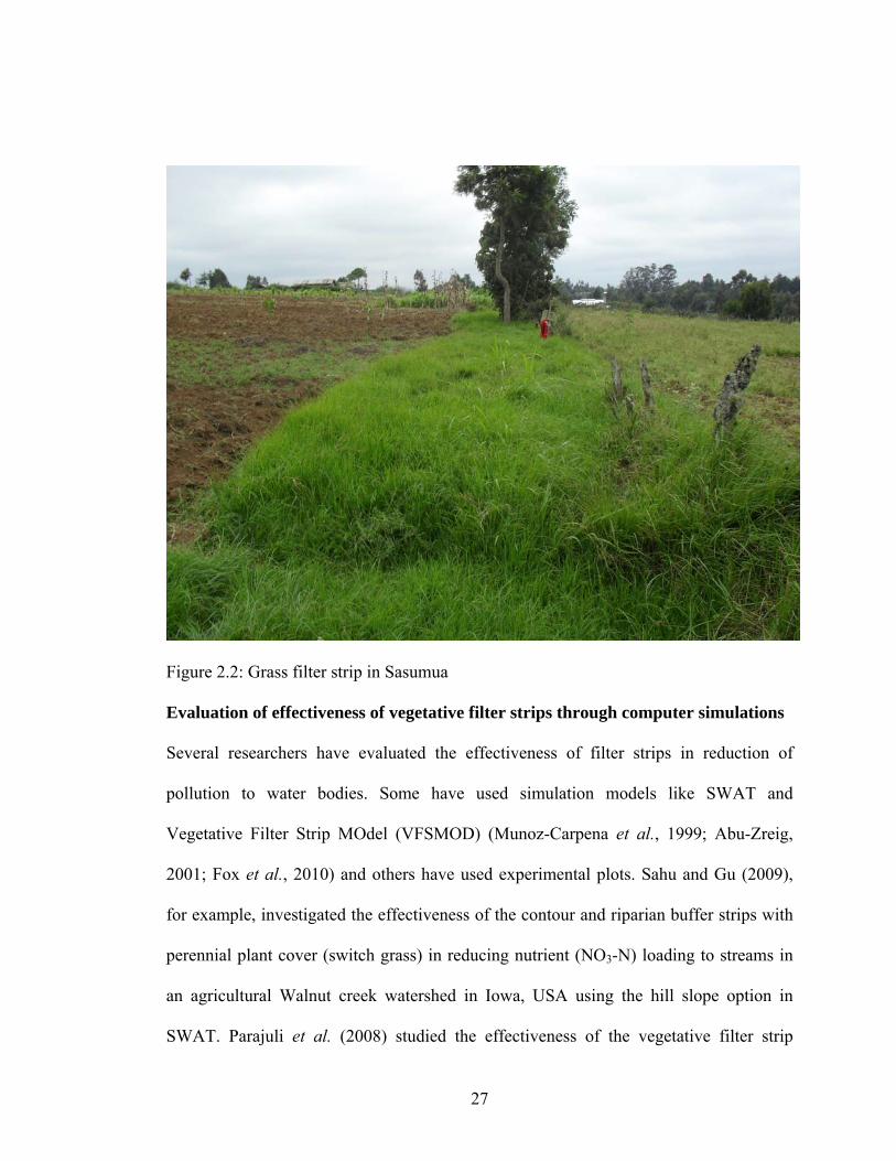
Figure 2.2: Grass filter strip in Sasumua

Evaluation of effectiveness of vegetative filter strips through computer simulations

Several researchers have evaluated the effectiveness of filter strips in reduction of

pollution to water bodies. Some have used simulation models like SWAT and

Vegetative Filter Strip MOdel (VFSMOD) (Munoz-Carpena et al., 1999; Abu-Zreig,

2001; Fox et al., 2010) and others have used experimental plots. Sahu and Gu (2009),

for example, investigated the effectiveness of the contour and riparian buffer strips with

perennial plant cover (switch grass) in reducing nutrient (NO3-N) loading to streams in

an agricultural Walnut creek watershed in Iowa, USA using the hill slope option in

SWAT. Parajuli et al. (2008) studied the effectiveness of the vegetative filter strip

27

lengths in removing overland process sediment and fecal concentrations using SWAT in

950 km2 upper Wakarusa watershed in northeast Kansas.

SWAT has a limitation in that it uses the same trapping efficiency for sediments,

nutrients and pesticides (Arabi et al., 2008). It also does not consider the effect of flow

concentration. Considering these limitations, White and Arnold, (2009), developed a

field scale Vegetative Filter Strip (VFS) sub-model for SWAT which would enhance the

ability of SWAT to evaluate the effectiveness of vegetative filter strips at the watershed

scale. They used data from literature studied in many different countries and simulations

from Vegetative Filter Strip MOdel (VFSMOD) (Munoz-Carpena et al., 1999). The sub-

model developed has three additional model parameters added as SWAT inputs: the

drainage area to VFS area ratio (DAFSratio), the fraction of the field drained by the most

heavily loaded 10% of the VFS (DFcon), and the fraction of the flow through the most

heavily loaded 10% of the VFS which is fully channelized (CFfrac), all are specified in

the Hydrological Response Unit (HRU) file.

Evaluation of effectiveness of vegetative filter strips through field experiments

Experimental plots have also been used to study the effectiveness of VFS in abatement

of pollution. Abu-Zreig et al. (2004) used 20 field experimental plots to study the

performance of VFS in reducing cropland runoff in Ontario, Canada, and to assess the

influence of filter length, the flow rate of incoming runoff and the type of vegetation.

They found that the filter width, had the greatest effect on sediment trapping, followed

28

by vegetation density and inflow rate. They also found that sediment-trapping efficiency

increased with the width of the filter strip. Borin et al. (2005) investigated the effect of a

6 m buffer strip in reducing runoff, suspended solids and nutrients from a field growing

maize, winter wheat and soybean in a field experiment in North-East Italy over a period

of 4 years. The study found that on average the total suspended solids reduced from 6.9

to 0.4 t ha−1. Duchemin and Hogue, (2009) evaluated the effectiveness of an integrated

grass/tree strip system (after one year of establishment) in filtering runoff and drainage

water from grain corn fields fertilized with liquid swine manure in Quebec Canada.

They reported that after the first year of the establishment of the experiment, the grassed

strips reduced runoff water volumes by 40%, Total Suspended Solids (TSS) by 87%

whereas the grass/tree strips reduced runoff volumes by 35%, TSS by 85%. They

however, note that the inclusion of trees in the grass trip did not indicate any significant

increase in filtering capacity. The trees were only 2 years old and not well established in

biomass.

These studies, whether through computer simulation or field experimental work, show

that VFS are quite effective in reducing non point source pollution. By altering some

variables such as the width, or the type of vegetation, the effectiveness of the filters can

be enhanced.

29

2.5 Structural conservation Practices

Structural measures often lead to a change in slope profile; are of long duration or

permanent; are carried out primarily to control runoff, wind velocity and erosion; often

require substantial inputs of labour or money when first installed; are often zoned on the

contour against wind direction; are often spaced according to slope; and involve major

earth movements and / or construction with wood, stone and concrete (Liniger et al.,

2002; Biamah et al., 1997). They involve design and construction of soil erosion control

structures. Examples include various types of terraces, diversion ditches, waterways,

grade stabilization structures and retention ditches. Some structural conservation

practices are briefly described next.

2.5.1 Terraces

Terraces are conservation structures which comprise of a series of horizontal ridges

made on a hillside (Neitsch et al., 2005). Terraces divide and shorten a long slope into a

series of shorter and more relatively level steps. The slope length is the terrace interval.

The reduced slope steepness and length allows water to soak into the ground and as a

result have less surface runoff and thus less soil erosion. There are different types of

terraces which include broad base and bench terraces. Broad base terraces consist of a

ridge which has a broad base and a flatter slope. The ridge is also cultivated and

therefore no agricultural land is lost. These terraces could also be classified as graded or

level. Bench terraces are constructed on steeper slopes where the ridge is steep and not

30

cultivated. They are made by re-shaping a steep slope to create flat or nearly flat ledges

or beds, separated by vertical or nearly vertical risers (Mati, 2007). In some cases

especially in East Africa, bench terraces are developed over time from other methods of

terracing such as stone lines, grass strips and trash lines or “fanya juu” terraces, so as to

reduce labor and avoid having to move large volume of soil (Mati, 2006)

Terraces have been studied on their effectiveness to reduce soil erosion and to reduce

surface runoff. Yang et al. (2009) assessed the impact of flow diversion terraces on

stream water and sediment yield in BlackBrook watershed in Canada by adjusting the

USLE_P factor in SWAT and found out that the implementation of the Flow diversion

terrace in the watershed reduced sediment yield by about 56% and also reduced water

yield by about 20% in summer growing seasons. Arabi et al. (2008) evaluated the

impacts of parallel terraces and other conservation practices on water quality in Indiana,

U.S.A. and found out that terraces, if implemented on 30% of the 7.3 km2 Smith Fry

watershed, could reduce sediment yield by about 15%. In this study they used SWAT to

simulate the impact of terraces. They represented terraces using a method they

developed of representing BMPs in SWAT. In their study the slope length, curve

number, and universal soil loss equation practice factor (USLE_P) were adjusted to

represent terraces. Gassman et al. (2006) and Santhi et al. (2006) varied USLE_P to

represent terraces in SWAT. Both studies found terraces to be very effective in reducing

sediment that cause water pollution.

31

Design of terraces- In the design of terraces, terrace spacing is an important parameter

to consider. The slope length is equal to the terrace interval (Neitsch et al., 2005) and is

equal to the horizontal interval. The horizontal interval method (equation 3) is one of the

methods used in the calculation of the terrace spacing (NRCS, 2009).

)/100(*)(H.I syxs += (3)

Where; H.I. is the horizontal interval (m) (SLSUBBSN in SWAT), s is slope of the HRU,

x is a dimensionless variable with values ranging from 0.12-0.24 and y is also a

dimensionless variable with values between 0.3 and 1.2. Values of y are influenced by

soil erodibility, cropping system and crop management systems. The low value of 0.3 is

used for highly erodible soils with tillage systems that provide little or no residue cover

while the high value of 1.2 is used for erosion resistant soils with a tillage system that

leave a large amount of residue (3.3 tons/ha) on the surface (NRCS, 2009; Arabi et al.,

2008). This variable is thus related to the USLE erodibility factor (USLE_K) and USLE

cover management factor, USLE_C. Typical y factor values are given in Table 2.

32

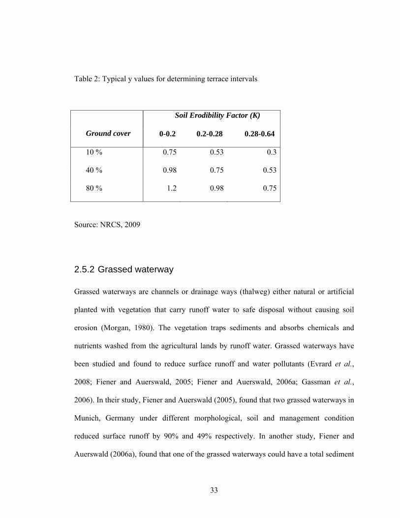
Table 2: Typical y values for determining terrace intervals

Soil Erodibility Factor (K)

Ground cover 0-0.2 0.2-0.28 0.28-0.64

10 % 0.75 0.53 0.3

40 % 0.98 0.75 0.53

80 % 1.2 0.98 0.75

Source: NRCS, 2009

2.5.2 Grassed waterway

Grassed waterways are channels or drainage ways (thalweg) either natural or artificial

planted with vegetation that carry runoff water to safe disposal without causing soil

erosion (Morgan, 1980). The vegetation traps sediments and absorbs chemicals and

nutrients washed from the agricultural lands by runoff water. Grassed waterways have

been studied and found to reduce surface runoff and water pollutants (Evrard et al.,

2008; Fiener and Auerswald, 2005; Fiener and Auerswald, 2006a; Gassman et al.,

2006). In their study, Fiener and Auerswald (2005), found that two grassed waterways in

Munich, Germany under different morphological, soil and management condition

reduced surface runoff by 90% and 49% respectively. In another study, Fiener and

Auerswald (2006a), found that one of the grassed waterways could have a total sediment

33

reduction of 93% over a period of 8 year of observation. Evrard et al. (2008) reported

that a 12 hectare grassed waterway reduced about 93% of sediment discharge in the

Belgian plateau belt over a monitoring period of 2002-2004.

These studies show that grassed waterway is an important and effective management

option to abate water pollution. Grassed waterways are structural BMPs and thus other

than the roughness offered by the vegetation, other parameters like the cross section, the

grade and the hydraulic properties of the thalweg also affects their effectiveness in

reducing surface runoff and trapping of pollutant to certain degrees. Fiener and

Auerswald, (2005) reported that wide, flatted bottom and long grassed waterway

efficiently reduced runoff volume and peak discharge rates and that slope and soil

conditions had little effect.

Channel Manning’s coefficient, channel cover and channel erodibity are some of the

factors that affect the effectiveness of the channel in trapping the sediments and reducing

degradation of the channel. Several studies have been done to determine these factors.

For example, Fiener and Auerswald (2006a), suggested that for dense grasses and herbs

under non submerged runoff condition, the channel Manning’s coefficient varies

between 0.3 and 0.4 s m-1/3 over the year provided the grass or herb do not bend or

break. Bracmort et al. (2006) used a channel Manning coefficient value of 0.24 s m-1/3

to represent grassed waterway in good condition in Black Creek watershed in Indiana

34

U.S.A while Arabi et al. (2008), suggested a value of 0.1 for grassed waterway in poor

conditions. Fiener and Auerswald, (2006b) used a value of 0.35 s m-1/3.

2.6 Soil and water conservation in Kenya

The soil conservation service in Kenya was started in 1930’s when the land which was

mainly occupied by European settlers had serious erosion problems that warranted

immediate attention. The government studied the situation and recommended that

practicing soil conservation was a must from 1937 (Biamah et al., 1997). In 1938, a soil

conservation service was introduced (Kamar, 1998). At that time, the government

mostly emphasized on simple cross-slope barriers such as trash-lines, rows of stones and

vegetative strips. African farmers then practiced conservation techniques such as shifting

cultivation, trash-lines and simple terracing. A number of conservation policies and

strategies were later introduced and strongly enforced administrative and agricultural

extension personnel employed to ensure compliance. Anybody who did not comply was

punished or prosecuted. Such conservation policies included, discouraging ploughing on

steep land, contour planting and ploughing, stopping cultivation along water courses,

encouraging terracing, planting trees on the hillsides, planting Napier grass, controlling

forest clearing and promoting de-stocking. Immediately after independence, soil

conservation practice was very low. The rapid drop in soil conservation practices then

was mainly because of reaction of farmers who believed that soil conservation activities

were part of colonialism. The use of force to do conservation activities was stopped after

independence. The effect of this was that most activities stopped, conservation structures

35

such as terraces were not maintained, and many were even destroyed. Steep slopes under

good vegetation cover were cleared for cultivation, forests were cut down for timber,

building materials and fuel wood and closed grazing areas were reopened. This saw soil

erosion features started re-appearing. The main focus of the new government then was

settling of landless people in the then newly created settlement schemes. Although there

have been several attempts to address the problem of soil erosion by the post

independence government with the help of international assistance, such as Kenya

National Soil Conservation Project in 1974, soil erosion is still a major problem. The

population pressure has strained the land resources and cultivation is practiced with little

regard of soil conservation (Kamar, 1998; Biamah et al., 1997).

2.7 Hydrological modeling

A model is simply an abstraction of a real system. Models are built for a specific

purpose which could be prediction, exploratory analysis, communication or learning.

Models are based on scientific knowledge and the information derived from them is used

to aid decision making. In natural resource management, it is a common practice to build

models to predict, in space or time, the states of the system to be managed. Hydrologic

models are used to investigate and aid in understanding the complex relationship

between climate and water resources (Singh and Frevert, 2002) and partitions water into

various pathways of the hydrological cycle.

36

Based on process description, models can be classified as either empirical (black box) or

physically based model (Refsgaard, 1996). An empirical model does not consider the

physical laws of the underlying watershed processes. They only reflect the relation

between the input and outputs. Physically-based models describe the natural system in a

watershed using mathematical representation of flows of mass and energy. Models can

also be classified as either lumped or distributed depending on the spatial representation

of parameters and variables. A lumped model is one where a watershed is regarded as

one unit where the variables and the parameters are represented by average values for

the whole watershed while a distributed model takes into account the spatial variation of

all variables and parameters.

Refsgaard, (1996) gives the following steps that are involved in hydrologic modeling

process. The first step is to evaluate the problem that need to be solved and then look

around to find if there is an existing model that can solve the problem or a new model

may need to be developed. If a model is selected from existing ones, it should be able to

give an acceptable solution to the problem or produce desirable outputs. The next step

involves model setup. This involves delineation of the watershed, setting boundary and

initial conditions, feeding the input data and parameterization. The model is then

calibrated and validated using measured data. Model calibration involves manipulation

of a specific model to reproduce the response of the watershed under study within a

range of the desired accuracy. This can be done by trial and error estimation of model

parameters or automatically using developed algorithms. Model validation involves the

37

application of the calibrated model without changing the parameters set in the

calibration procedure. The model should be able to simulate the processes in another

period different from the one used in the calibration process. For example, a validated

model should be able to reproduce measured stream flow data series for a chosen period

which is different from the period of the stream flow data used in the calibration

exercise. The model performance is usually tested during the calibration and validation

exercises by statistically comparing the goodness of fit of the simulated output and the

observed (measured) data. Coefficient of determination, R2, bias, Nash Sutcliffe

Efficiency (NSE) (Nash and Sutcliffe, 1970) and Root Mean Square Error (RMSE) are

the common statistics used to measure model performance (Singh and Frevert, 2002;

Sang, 2005). Once a model is satisfactory calibrated and validated, it can be used for

desired simulations.

2.8 SWAT overview: Sediment and hydrology theory

In SWAT, a watershed is partitioned into sub-basins. The number of sub-basins will be

determined by the ‘critical source area’ chosen by the user. Critical source area is the

minimum area required by the model for the initiation of channel processes (Bracmort et

al., 2006; Arabi et al., 2008). The sub-basins are further divided into HRUs. A HRU has

unique land use, soil attributes and management.

38

Water balance is the driving force behind all the processes in a watershed in SWAT.

Therefore accurate predictions of pesticides, sediments and nutrients will only be

possible if hydrological processes are well simulated in the model. Hydrological cycle of

a watershed is divided into land phase and the routing phase of the hydrological cycle.

The former controls the amount of water, sediments, nutrients and pesticides that enter

the main channel in each sub-basin while the later deals with their movement through

the channel network of the watershed to the outlet (Neitsch et al., 2005). The land phase

of hydrological cycle in SWAT is based on equation 4;

)(1

gwseepas

t

tot QWEQRSWSW −−−−+= ∑

= (4)

Where, SWt is the final soil water content (mm), SWo is the initial water content on day i

(mm), t is time in days, R is amount of precipitation on day i (mm), Qs is the amount of

surface runoff on day i (mm), Ea is the amount of evapotraspiration on day i (mm), Wseep

is the amount of water entering the vadose zone from the soil profile on day i (mm) and

Qgw is the amount of return flow on day i (mm)

2.8.1 Climatic inputs for SWAT

Climate provides the moisture and the energy inputs that control the water balance

(Neitsch et al., 2005). SWAT requires several climatic data which include daily

precipitation, maximum and minimum temperature, solar radiation data, relative

humidity, and wind speed data. These climatic variables can be input from measured

39

records or can be simulated by the weather generator. SWAT includes a weather

generator, WXGEN, to generate climate data or fill in gaps in the measured records

(Neitsch et al., 2005). The weather generator requires average monthly climate values

analyzed from long-term measured weather records and generates daily weather values

for each sub-basin.

2.8.2 Calibration of SWAT model

Calibration can be done manually or automatically in SWAT. The model can be

calibrated for stream flow, sediments and chemicals (Neitsch et al., 2005). Automatic

calibration requires use of good observed data and is very convenient for gauged

catchment with long-term continuous data. However, in many developing countries like

Kenya, hydrological data is not oftenly collected for many rivers and even where they

are collected, data management is quite a challenge. Researchers working in such

watersheds face a big challenge in calibration and validation of hydrological.

Appreciating this problem, Ndomba et al. (2008) validated the applicability of SWAT

model in a data scarce catchment in Pangani River basin in Tanzania. Based on the

sensitivity analysis done, the study found that hydrological controlling parameters could

be identified using SWAT runs without observed data. From their study they suggest

that SWAT model can be used in ungauged catchment for identifying hydrological

controlling parameters. In fact, SWAT is a physically based distributed model and was

designed for use in ungauged watershed (Gassman et al., 2007) making it a suitable

40

model for watersheds with little or no data. Thus the model has been used for many

studies in similar situations where stream flow and/or pollutants (sediments, chemicals

and nutrients) data was not available. For example, Santhi et al. (2006) used SWAT to

evaluate the impact of implementation of Water Quality Management Plans on non-

point source pollution in West Fork watershed of Trinity River basin in Texas, U.S.A.

They didn’t have good continuous sediment data. They used few grab samples data,

expertise and experience from previous studies to calibrate the model for sediments. In a

recent study, Galvan et al. (2009) used SWAT model to generate reservoir inflow that

they used as observed stream flow for the calibration of the model in Meca River basin

in Spain.

2.8.3 Hydrology in SWAT

From precipitation, the water can be intercepted by the vegetation or fall to the soil

surface. The water that is intercepted by the vegetation (Canopy storage) is made

available for evaporation. The water that falls on the soil surface can either infiltrate or

flow as surface runoff. For each HRU, surface runoff is predicted separately and routed

to get the total runoff for the entire watershed. Surface runoff volumes and peak runoff

rates are calculated for each HRU. Peak runoff rate is calculated using Modified rational

formula (equation 17). SWAT either uses the SCS curve number method or Green &

Ampt infiltration method to compute surface runoff volumes. The curve number method

was used for this study and the surface runoff is calculated from equation 5;

41

)()( 2

SIRIR

SR aday

adayQ +−−= (5)

Where QSR is the accumulated runoff (mm), Rday is rainfall depth for the day (mm) Ia is

initial abstraction (surface storage, interception and infiltration prior to runoff (mm)- this

is estimated as 0.2 S and S is the retention parameter (mm) which is calculated;

)10(4.25 1000 −= CNS (6)

Where CN is SCS Curve Number of the day and is a function of soil permeability, land

use and antecedent soil moisture condition.

Runoff will occur only when Rday >Ia

The water that infiltrates into the ground can be stored in the soil as soil moisture and

later removed through evepotranspiration or could move laterally in the soil profile to

contribute to stream flow or can percolate below the soil profile and recharge the

aquifer. Evapotranspiration is a collective term that includes all the processes by which

water in the earth’s surface is converted to water vapour and includes water that

evaporates from the plant canopy, transpiration, sublimation, and evaporation from the

soil (Neitsch et al., 2005). Evapotranspiration is usually limited by the availability of

enough moisture in the soil and is also affected by other factors such as weather

parameters, vegetation (crop) factors, and management and environmental conditions

42

(Allen et al., 1998). Thus, the concept of potential evapotranspiration was developed to

study the evaporative demand of the atmosphere independent of plant type, plant

development and management practices. In SWAT, potential evapotranspiration is first

determined, and then actual evapotranspiration is then determined by calculation of

evaporation, transpiration and sublimation separately. SWAT gives the flexibility of

using any of the three methods of calculating potential evapotranspiration incorporated

in the model. The methods are; Penman-Monteith, Priestly and Taylor and the

Hargreaves methods.

Lateral subsurface flow also known as the interflow, is the water that flows through the

soil profile below the soil surface and above the saturation zone and contributes to the

stream flow. SWAT uses a kinematic storage model to predict lateral flow in each soil

layer. Hydraulic conductivity, slope and soil water content are the governing parameters

in the model (Neitsch et al., 2005).

The water that percolates below the soil profile moves through the vadose zone and

recharges the shallow and/or deep aquifer. This water is partitioned between the shallow

and the deep aquifer. Shallow aquifer contributes the base flow to the streams. Return

flow to the stream system and evapotranspiration from deep‐rooted plants (termed

“revap”) can occur from the shallow aquifer.Water that recharges the deep aquifer is

assumed lost from the system (Gassman et al., 2007).

43

Water routing- In channels (streams and ditches) Manning’s equation (25) is used to

define the rate and velocity of flow in SWAT. Water is routed through the channel

network using the variable storage routing method (Williams, 1969) or the Muskingum

river routing method. Both of these methods are variations of kinematic wave model.

Muskingum river routing method was used for this study and is thus briefly explained.

The Muskingum routing method models the storage volume in a channel length as a

combination of wedge and prism storages (Figure 2.3) (Neitsch et al., 2005).

Figure 2.3: Prism and wedge storages in a reach segment (Neitsch et al., 2005)

A wedge is produced as a flood wave advances into the reach segment when the inflow

exceeds outflow. As the flood recedes, a negative wedge is produced when the outflow

exceeds inflow in the reach segment. The reach segment also contains a prism storage

formed by a volume of constant cross-section along the reach length (Figure 2.3). The

44

volume of prism storage can be expressed as a function of discharge, K .qout where K is

the ratio of storage to discharge and has the dimension of time. The volume of the wedge

storage can be expressed as K . X . (qin-qout) where X is a weighting factor that controls

the relative importance of inflow and outflow in determining the storage in the reach.

Therefore the total storage given by summing the wedge and the prism storages is given

in equation 7 below (Neitsch et al., 2005).

).(.. outinoutstored qqXKqKV −+= (7)

Where Vstored is the storage volume (m3), qin is the inflow rate (m3/s), qout is the discharge

rate (M3/s), K is the storage time constant for the reach and X is the weighting factor.

5.00.0 ≤≤ X

The weighting factor X is a function of the wedge storage and has a value of 0.0 for

reservoir type of storage and 0.5 for a full wedge while for rivers it falls between 0.0 and

0.3 with a mean value of 0.2.

When the storage equation 7 is incorporated in the continuity equation and simplified,

the resulting equation is

1,31,22,12, ... outininout qCqCqCq ++= (8)

45

Where qin,1 is the inflow rate at the beginning of the time step (m3/s), qin,2 is the outflow

rate at the end of time step (m3/s), qout,2 is the outflow rate at the end of the time step

(m3/s).

In terms of volume, both sides of equation 7 are multiplied by the time step and gives

1,31,22,12, ... outininout VCVCVCV ++= (9)

tXKXKtC Δ+−

−Δ= )1.(.2..2

1 (10)

tXKXKtC Δ+−

+Δ= )1.(.2..2

2 (11)

tXKtXKC Δ+−

Δ−−= )1.(.2)1.(.2

3 (12)

Where C1 + C2+ C3 = 1

Soil erosion- In SWAT, erosion and sediment yield are calculated using Modified

Universal Soil Loss Equation (MUSLE). The difference between MUSLE and Universal

Soil Loss Equation (USLE) is that USLE uses rainfall as indicator of erosive energy

while MUSLE uses the amount of runoff to simulate erosion and sediment yield. The

advantages of using MUSLE over USLE are; prediction accuracy of the model is

increased, the need of sediment delivery ratio is eliminated and estimates of sediment

46

yields for a single storm can be computed (Neitsch et al., 2005). The MUSLE equation

is given in equation 13;

CFRGLSPCKAqQSed USLEUSLEUSLEUSLEpeaks ×××××= 56.0)...(8.11 (13)

Where Sed is the sediment yield on a given day (tons/ha), Qs is the surface runoff

(mm/ha), qpeak is peak runoff rate (m3/s), A is Area (of HRU) (ha), KUSLE is the USLE

soil erodibility factor, CUSLE is the USLE cover management factor, PUSLE is the USLE

support factor, LSUSLE is the USLE topographic factor and CFRG is course

fragmentation factor

KUSLE, CUSLE, PUSLE and LSUSLE are as described in the USLE equation (1).

Effect of slope length on sediment yield

Slope length affects the topographic factor, LS as well the peak runoff rate. SWAT uses

MUSLE equation (13) to estimate soil erosion. The topographic factor, LS, is calculated

by equation 14 .

)065.0sin.56.4)(sin.41.65.()( 21.22 ++= hillhill

mLUSLE

hillLS αα (14)

Where; LSUSLE is topographic factor, Lhill is slope length which is equal to SLSUBBSN

in SWAT (m) and αhill is the angle of slope and exponent m is computed;

47

]).835.35exp[1(6.0 slpm −−×= (15)

Where; slp is slope of the HRU (m/m) and

hillslp αtan= (16)

Modified Rational method (equation 17) is used to model peak runoff rate in SWAT.

c

tcpeak t

AreaQq

×××

=6.3

α (17)

Where; qpeak is peak runoff rate (m/s), Q is surface runoff (mm), αtc is fraction of the

daily rainfall that occurs during the time of concentration, Area is sub-basin area in km2

and tc is the time of concentration for the sub-basin (hrs).

The time of concentration tc, is calculated as;

3.0

6.06.0

18 slpnL

t slpc ×

×= (18)

Where; Lslp = SLSUBBSN is slope length (m), n is Manning’s roughness coefficient and

slp is slope of the sub-basin (m/m).

48

In SWAT, the slope length,

Lhill =Lslp =SLSUBBSN (19)

By substituting equations 14, 17, 18, and 19 in the MUSLE equation (12), the total effect

of slope length (SLSUBBSN) on upland soil erosion can be estimated as (Arabi et al.,

2008);

mSLSUBBSNSLSUBBSNSed ×∝ ×− )56.06.0( =

)336.0( −∝ mSLSUBBSNSed (20)

Where; Sed is sediment yield computed in MUSLE equation (13).

From (13), it can be seen that the contribution of the slope length to the sediment yield

will be equal (unit) for any sub-basin length when m equals 0.336. Since exponent m

(computed from equation 15) depends on the slope of the sub-basin, a value of 0.336

will correspond to a slope of 0.023. Above this slope, a reduction in slope length would

have an overall reduction in soil erosion (Figure 2.4). However, below that slope, a

reduction in slope length would actually result in an increase in the simulated sediment

yield (Arabi et al., 2008). For that reason, terraces are best simulated for HRUs whose

average slope is above 2.3 %.

49

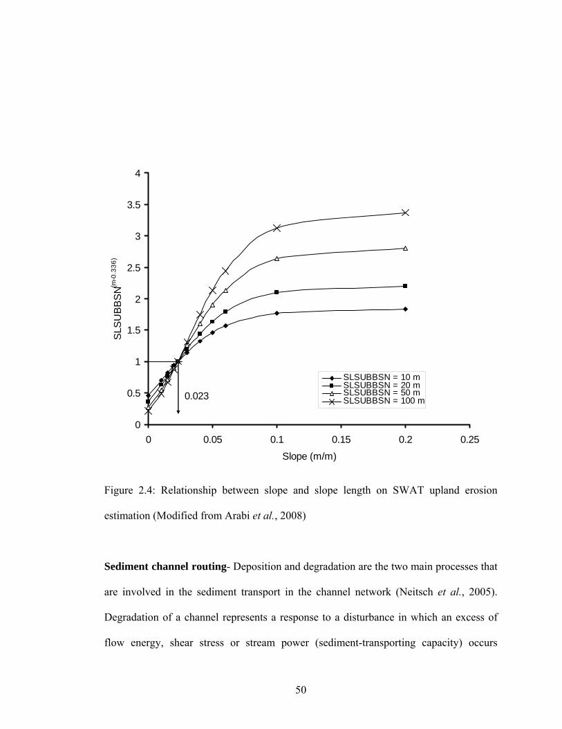
0

0.5

1

1.5

2

2.5

3

3.5

4

0 0.05 0.1 0.15 0.2 0.25

Slope (m/m)

SLS

UBB

SN(m

-0.3

36)

SLSUBBSN = 10 mSLSUBBSN = 20 mSLSUBBSN = 50 mSLSUBBSN = 100 m0.023

Figure 2.4: Relationship between slope and slope length on SWAT upland erosion

estimation (Modified from Arabi et al., 2008)

Sediment channel routing- Deposition and degradation are the two main processes that

are involved in the sediment transport in the channel network (Neitsch et al., 2005).

Degradation of a channel represents a response to a disturbance in which an excess of

flow energy, shear stress or stream power (sediment-transporting capacity) occurs

50

relative to the amount of sediment supplied to the stream (Simon and Rinaldi, 2006).

Degradation causes systematic bed-level lowering over a period of time can affect long

stream reaches, entire lengths of one stream, or whole stream networks. It is different

from scouring which is erosion of the stream bed or bank and limited in magnitude as

well as in spatial and temporal extent. Scour can occur over periods of hours to days and

affects localized areas in response to storm flow (Simon and Rinaldi, 2006). Deposition

occurs when the sediment in the water settle on the river bed as a result of reduced

transport capacity. In SWAT degradation is modeled as a function of stream power

determined by channel slope and flow velocity (equation 25). If the sediment

concentration in the water is greater than the maximum sediment that can be transported

in the flow (equation 27), then sediment deposition occurs. The reverse is true for the

degradation process.

Only the main hydrological, soil erosion and sediment transport process are highlighted

here. Many of these processes have other sub processes which are not highlighted. Other

than climate, hydrology and sediment (soil erosion), other components of SWAT include

plant growth, nutrients, pesticides, bacteria, pathogens and land management. Complete

descriptions of theory and underlying processes and governing equations in SWAT can

be found in Neitsch et al. (2005). Nutrients, pesticides bacteria and pathogens were not

modeled in this study.

51

CHAPTER 3

MATERIALS AND METHODS

This chapter describes the materials and methods used to simulate soil and water

conservation practices. The study was carried out in Sasumua watershed, Kenya. SWAT

model was first calibrated and validated for Sasumua and then used to simulate the

conservation practices. The Sasumua reservoir inflow data calculated from reservoir

water balance was used for calibration and validation of the model. Field visits and

farmers interviews were done to get the land management information necessary for the

model setup. The major inputs for the SWAT model include, Digital Elevation Model

(DEM), soil data, land use and land management, weather data (rainfall, temperature,

relative humidity, radiation and wind speed) and Weather generator information which

require statistics of weather pattern over a period of time. Stream flow and water quality

data such as sediments may also be used for model calibration and validation. Input data

to the model were collected from different sources and are described in the chapter.

3.1 Data collection

3.1.1 DEM, Land use/Land cover and Soil Data

The data collected for this study included, a DEM with a spatial resolution of 10 m, a

land use/land cover map generated using digital image classification of aster satellite

52

images of 2007 ( both from World Agroforestry Center, Nairobi). Soil data for the

watershed were extracted from the Digital Soil and Terrain Database of East Africa

(SOTER) (FAO, 1997). Soil properties required by the model are hydrological soil

groups, soil depth, textural fractions, saturated hydraulic conductivity, available water

capacity, bulk density and organic matter content for various soil layers. Some of these

parameters were derived directly from the SOTER database while others were found in

literature.

3.1.2 Climatic data

Twenty seven years of rainfall data (1970-1996) for meteorological station number

9036188 at the dam site area and twenty one years (1970-1990) for south Kinangop

forest rainfall station were used. Wind speed data for the Sasumua dam site station was

used. Wind speed data was required in the calculation of evapotranspiration using the

Penman Monteith equation by the model. For the other weather parameters such as

temperature, solar radiation and humidity were simulated by the weather generator in

SWAT. SWAT includes WXGEN weather generator model to generate climate data and

to fill in gaps in the measured records (Neitsch et al., 2005). Statistical climate data of a

station in or within the vicinity of the watershed is required for the weather generator.

The data for this was obtained from Kimakia Forest meteorological station (station ID

0936233) neighboring the Sasumua watershed.

53

3.1.3 Reservoir levels data

Stream flow data needed to calibrate the model was not available for the gauging

stations in the watershed. Reservoir levels data was collected from the Nairobi Water

and Sewerage Company offices at the dam site and were used for the calibration and

validation of the model.

3.1.4 Site visits and farmer interviews

To get the baseline conditions that are necessary for the modelling purposes, site visits to

the watershed were made to assess the condition of the land and water resources. During

the site visits twenty farmers from the watershed were selected and interviewed (Figure

3.1). The criteria for selection of the farmers were on the basis of the location of the land

in terms of topography, farm size and also the wealth of the farmer. These criteria

ensured that the farmers selected were representative of the watershed. Questionnaires

(Appendix 2) were administered to the farmers. For this study, the information that

needed to be extracted from the farmers was the crops grown and the cropping pattern

and also to assess the existing soil and water conservation measures on the farms. This

baseline information was necessary for model setup before simulation of conservation

practices. Table 3 gives a one-year rotation management operation that was modelled for

the agricultural part of Sasumua Sub-watershed based on the interviews from the

farmers.

54

Figure 3.1: Interview with one of the farmers

55

Table 3: Management operations modelled for the agricultural land

Operation Date

Planting potatoes

Harvesting (harvest and kill)

Planting cabbages

Harvesting (harvest and kill)

Planting potatoes

Harvesting (harvest and kill)

1st March

31st May

15th June

15th September

1st October

31st December

3.2 Model setup for base scenario

The DEM, Land use and soil maps were configured to a similar projection (Custom

Traverse Mercator, WGS 1984). The watershed was subdivided into 62 sub-basins

(Figure 3.2).

56

## #

#

33 8

9 6

3

5

18

61 62

28

16

42

1

14

40

37

43

34

51

60

54

2

57

22

41

7

58

4438

48

10

30

50

17

36

24

46

26

11

2945

52

12

25

20

27

13

39

56

15

49

21

4

53

3231

47

55

19

35

23

59

1 0 1 2 3 4 Kilometers

SubbasinsReservoirStreamsChania tunnel

# IntakesKiburu pipe

N

Figure 3.2: Sub-basins as simulated in SWAT model

Dominant land use and soil was used as the criteria for HRU definition. Dominant land

use and soil criteria mean that a HRU is modeled with only a single land use/land cover

and soil. This is normally the land use or the soil with the largest percentage in that

HRU. The land use/land cover and soils with the smaller percentages are ignored for that

particular HRU. Recorded rainfall data for Sasumua meteorological station for Kinangop

forest rainfall stations were used. Wind data for Sasumua metrological station was used.

All the other parameters i.e. (temperature, solar radiation and relative humidity, were

simulated from weather generator data used for Kimakia Forest metrological station.

57

Management operations were scheduled by dates. In SWAT operations can be scheduled

either by heat units or by dates (Neitsch et al., 2005).

The SCS Curve number method (equation 5) was used to model the surface runoff.

Muskingum routing method (equations 7) was used to rout the water through the streams

and Penman Monteith equation was used to calculate the evapotranspiration.

For the watershed delineation in the model, the main outlet was chosen to be at the

confluence of Rivers Chania and Sasumua which is slightly downstream of the reservoir.

This was necessary so that the model would include the Chania and Kiburu sub-

watersheds in the watershed boundary. Kiburu sub-watershed has its intakes falling in

sub-basins 25, 27 and 28 while Chania has its intake at sub-basin 33. To exclude the

flow from the sub-basins that are downstream of the intakes at Chania and Kiburu sub-

watershed, the stream flow and sediment outputs at the outlets of sub-basins 25, 27 and

28 for Kiburu and 33 for Chania were summed up with that of the outlet of Sasumua

sub-watershed at sub-basins 57 and 59.

3.3 Parameter Sensitivity analysis

In order to guide the calibration process, parameter sensitivity analysis was done to

identify parameters which had the most impact on model outputs.

58

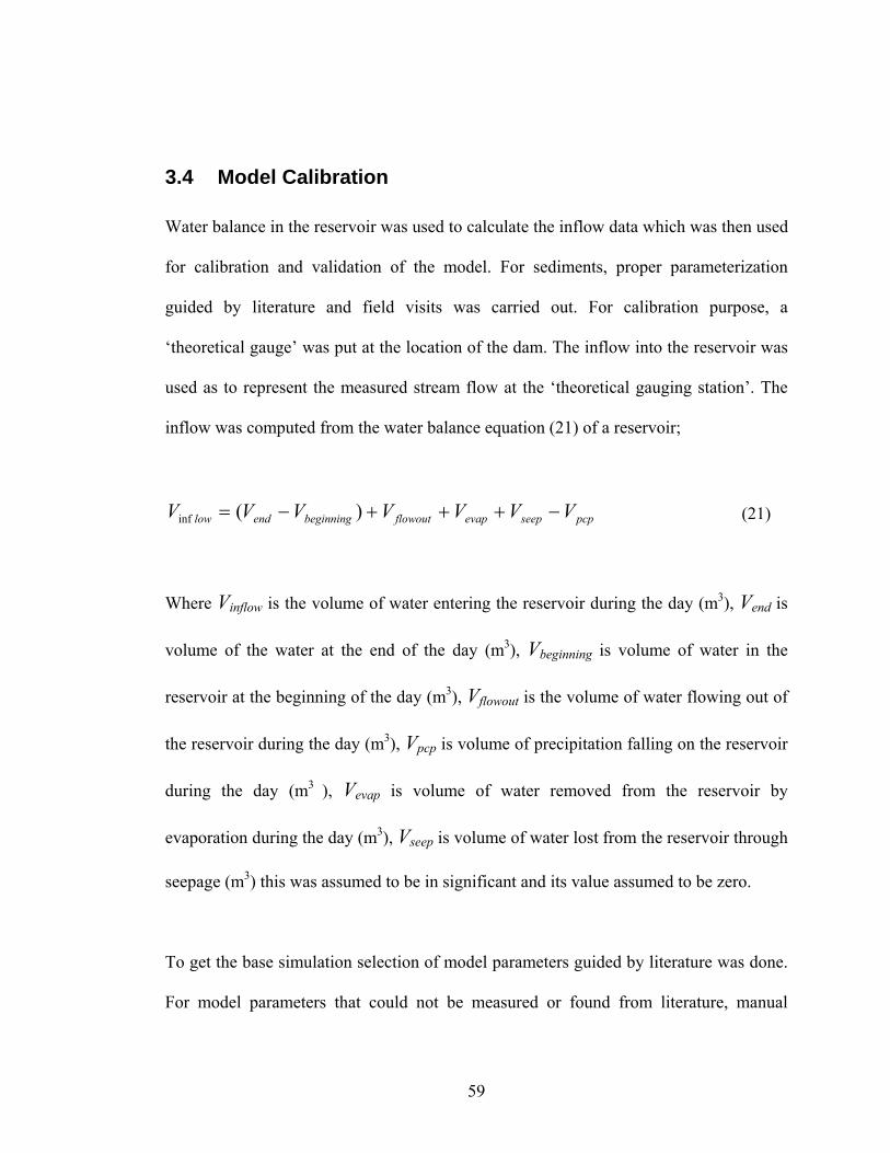
3.4 Model Calibration

Water balance in the reservoir was used to calculate the inflow data which was then used

for calibration and validation of the model. For sediments, proper parameterization

guided by literature and field visits was carried out. For calibration purpose, a

‘theoretical gauge’ was put at the location of the dam. The inflow into the reservoir was

used as to represent the measured stream flow at the ‘theoretical gauging station’. The

inflow was computed from the water balance equation (21) of a reservoir;

pcpseepevapflowoutbeginningendlow VVVVVVV −+++−= )(inf (21)

Where Vinflow is the volume of water entering the reservoir during the day (m3), Vend is

volume of the water at the end of the day (m3), Vbeginning is volume of water in the

reservoir at the beginning of the day (m3), Vflowout is the volume of water flowing out of

the reservoir during the day (m3), Vpcp is volume of precipitation falling on the reservoir

during the day (m3 ), Vevap is volume of water removed from the reservoir by

evaporation during the day (m3), Vseep is volume of water lost from the reservoir through

seepage (m3) this was assumed to be in significant and its value assumed to be zero.

To get the base simulation selection of model parameters guided by literature was done.

For model parameters that could not be measured or found from literature, manual

59

calibration of stream flow was carried out. The period between 1988 and 1993 was used

for calibration. The first two years were used as the warm up period.

After running the model, the simulated outflows were plotted along the ‘observed’

stream flow. Both visual and statistical methods were used to assess the goodness of fit

between the simulated and the observed stream flow. Coefficient of determination (R2)

was used to numerically test the model performance. R2 varies between 0 and 1 with one

being ideal for a perfect fit. An R2 of 0.5 and above was considered reasonable for this

study considering the accuracy of the data used.

3.5 Model Validation

To demonstrate that the calibrated model was capable of making accurate predictions,

the model was validated. The reservoir inflow data was used for the validation just as in

the case of calibration. The model was validated by data for the period between 1994

and 1997. Both calibration and validation periods were chosen to correspond to the time

when there was relatively good data for calculation of the reservoir water balance

components. During validation process, the model parameter values set during the

calibration were maintained constant. The resulting stream flow (simulated) was

compared visually in a graph with the observed stream flow. Coefficient of

determination was also determined.

60

3.6 Simulation of soil and water conservation Practices

Sasumua sub-watershed (Figure 1.1) which is mainly agricultural was the only portion

of the watershed which was considered for the simulation of the conservation practices.

Chania and Kiburu sub-watersheds which are under forest were left out since the forest

provides enough soil cover. For Sasumua sub-watershed, the main outlet at the dam was

considered at the outlet of sub-basins 57 and 59 (Figure 3.2) which capture the flow and

pollutants from the entire sub-watershed. The methodology used for the simulation of

conservation practices in this study is based mainly on the methodology developed for

simulation of conservation practices in SWAT by Arabi et al. (2008). In this study, the

agronomic and vegetative conservation practices considered were the contour farming

and vegetative filter strips. Bench terraces and grassed waterway were simulated in case

of structural conservation practices. Two more simulations were done to compare

management scenarios in the watershed. The first management scenario simulated a

situation where less intensive cultivation in agricultural lands and proper managed

grazing in grasslands are practiced. The second management scenario simulated a

situation where intensive cultivation in agricultural lands and overgrazing in grasslands

would cause degradation of the watershed.

3.6.1 Vegetative Filter strips

The width of edge-of-field filter strip parameter (FILTERW) in SWAT was adjusted to

simulate this conservation practice. The filter strips were simulated for all the sub-basins

in the agricultural part of Sasumua sub-watershed except sub-basins 57, 58 and 60 where

61

a wide riparian buffer exists (Figure 3.2). This buffer is managed by Nairobi City Water

and Sewerage Company NCWSC and was left to protect the reservoir from siltation.

The width of the filter strip was increased at interval of 5 meters from 0 to 35 m. Only

the parameter FILTERW was adjusted for each simulation. The sediment loading at the

outlet of sub-basins 57 and 59 (reference sub-basins) for various widths of filter strip

was determined. The effectiveness on the filter strips in the reduction of the sediment

yield is based on the trapping efficiency.

3.6.2 Contour farming

To represent contour farming, the CN was decreased by three units from the

calibration/parameterization values according to the method developed by Arabi et al.

(2008). USLE_P was adjusted depending on the slope of the HRU according to Table 4

given by Neitsch et al. (2005). The table gives recommended USLE_P values for

contour farming, strip cropping and terracing. The USLE_P values for the target sub-

basins in the agricultural part of the sub-watershed were reduced from the base

simulation value of 0.85.

62

Table 4: USLE-P values for contour farming, strip cropping and terracing

USLE_P

Land slope (%)

Contour

farming

Strip cropping Terracing

Type 1a Type 2b

1 to2 0.60 0.30 0.12 0.05

3 to 5 0.50 0.25 0.10 0.05

6 to 8 0.50 0.25 0.10 0.05

9 to 12 0.60 0.30 0.12 0.05

13 to 16 0.70 0.35 0.14 0.05

17 to 20 0.80 0.40 0.16 0.06

21 to 25 0.90 0.45 0.18 0.06

a Type 1: graded channel sod outlet

b type 2: Steep backslope underground outlets

Source: (Weischmeier and Smith, 1978)

To further evaluate how much the a combination of the filter strips and contour farming

would have on the sediment yield and stream flow, another simulation was run with a 5

63

m filter strip width and the CN and USLE_P values selected to represent the contour

farming.

Only the sub-basins in the agricultural part of the watershed in the Sasumua sub-

watershed were included in the simulation of contour farming.

3.6.3 Bench terraces

To simulate bench terraces in SWAT, slope length within sub-basin (SLSUBBSN),

USLE_P, and CN were adjusted (Arabi et al., 2008). In SWAT, slope length is

represented by the parameter SLSUBBSN. Adjusting this parameter downwards

represented reduced slope length. The reduced soil loss was factored in by reducing the

USLE_P in the Modified Universal soil loss equation used to model soil erosion in the

SWAT model. Implementation of bench terraces would affect all these processes

together and thus all the parameters were adjusted simultaneously in a single run.

The CN values were reduced by 7 units from the calibration values for each HRU. The

value of 7 was selected based on the values for CN for different practices given in

Neitsch et al. (2005). USLE_P values for terracing type 1 (graded channels sod outlets)

in Table 4 were used depending on the average slope of the HRU. To determine the

appropriate slope length for each HRU after implementation of bench terraces,

Horizontal Interval method (section 2.5.1) was used. The original slope length calculated

by the model from the DEM was reduced to the slope length calculated by the

64

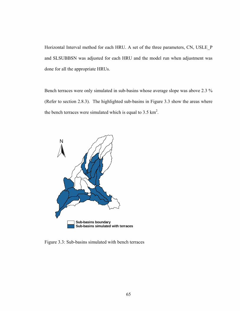
Horizontal Interval method for each HRU. A set of the three parameters, CN, USLE_P

and SLSUBBSN was adjusted for each HRU and the model run when adjustment was

done for all the appropriate HRUs.

Bench terraces were only simulated in sub-basins whose average slope was above 2.3 %

(Refer to section 2.8.3). The highlighted sub-basins in Figure 3.3 show the areas where

the bench terraces were simulated which is equal to 3.5 km2.

Sub-basins simulated with terracesSub-basins boundary

N

Figure 3.3: Sub-basins simulated with bench terraces

65

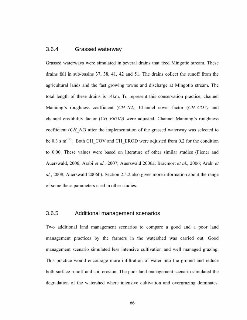
3.6.4 Grassed waterway

Grassed waterways were simulated in several drains that feed Mingotio stream. These

drains fall in sub-basins 37, 38, 41, 42 and 51. The drains collect the runoff from the

agricultural lands and the fast growing towns and discharge at Mingotio stream. The

total length of these drains is 14km. To represent this conservation practice, channel

Manning’s roughness coefficient (CH_N2), Channel cover factor (CH_COV) and

channel erodibility factor (CH_EROD) were adjusted. Channel Manning’s roughness

coefficient (CH_N2) after the implementation of the grassed waterway was selected to

be 0.3 s m-1/3. Both CH_COV and CH_EROD were adjusted from 0.2 for the condition

to 0.00. These values were based on literature of other similar studies (Fiener and

Auerswald, 2006; Arabi et al., 2007; Auerswald 2006a; Bracmort et al., 2006; Arabi et

al., 2008; Auerswald 2006b). Section 2.5.2 also gives more information about the range

of some these parameters used in other studies.

3.6.5 Additional management scenarios

Two additional land management scenarios to compare a good and a poor land

management practices by the farmers in the watershed was carried out. Good

management scenario simulated less intensive cultivation and well managed grazing.

This practice would encourage more infiltration of water into the ground and reduce

both surface runoff and soil erosion. The poor land management scenario simulated the

degradation of the watershed where intensive cultivation and overgrazing dominates.

66

This practice would impede infiltration of water and increase surface runoff and

subsequent soil erosion.

Good management scenario was simulated by decreasing the CN by 6 units from the

base simulation case. The poor management scenario was done by increasing the CN by

6 units from the base simulation scenario. Decreasing the curve number will increase the

infiltration in the curve number method and thus increase the surface runoff. The vice

versa is true.

67

CHAPTER 4

RESULTS AND DISCUSSION

In this chapter the results of the study are presented and discussed. The result of the

farmer interview whose information was used during model setup is presented first. The

output of the sensitivity analysis, calibration and validation of SWAT model is then

presented. Lastly the results and discussion of simulation of soil and water conservation

practices on water and sediment yield follow.

4.1 Farmer interviews

4.1.1 Land use/land cover

From the interview with the farmers, it was found out that Irish potato is the main crop

grown in the area as it can be seen in Figure 4.1. Irish potato is grown in rotation with

cabbages and there are three growing seasons in a year mainly. Similar results have been

observed in other studies (Bhattarai, 2009). This information was used in the model

setup to simulate land management operations (Table 3). Most farmers in the watershed

practice shift cultivation where they grow crops on one section of their farms and leave

other sections as fallow where they normally graze (Figure 4.1). After several years of

cultivation, the farmers leave the land and open new land which had been left fallow.

68

Figure 4.1 shows that 66% of the land as fallow. The percentages were based on the total

area of the land owned by the farmers interviewed. Twenty farmers were interviewed

and the size of the land they own was one factor considered during selection of the

farmers. Some farmers (majority) own as small as a quarter acre of land while others

have as much as 100 acres. Farmers with small pieces cultivate their entire piece of land

and don’t practice shift cultivation. Farmers with big chunks of land leave large parts of

their land fallow. However, these farmers are only few and therefore, the percentage

represented by the fallow land in Figure 4.1 only represents the percentage of the twenty

farms but not for the entire watershed.

69

woodlot5%

oat3%

others1%

Irish potato11%

cabbage8%

Maize4%

Napier grass1%

pasture/fallow66%

peas1%

Figure 4.1: percentage Land use (based on 20 farms visited)

4.1.2 Soil conservation practices in Sasumua

Field visits to the watershed and interview with farmers revealed that there is minimum

soil conservation practiced in the area. Some of the soil conservation measures found in

the watershed were bench terraces and fanya juu terraces in very few farms on the steep

slopes. On the flat area of the watershed where flooding happens during the rainy

season, drainage ditches are common and farmers usually plant napier grass for fodder

on the embankment along the drainage channels (Figure 4.2). Grass strips are also found

in few farms in the watershed. At the individual farms where some of these

conservation measures are undertaken, they have managed to control soil erosion to

70

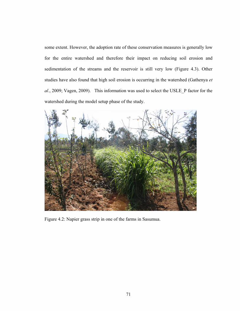
some extent. However, the adoption rate of these conservation measures is generally low

for the entire watershed and therefore their impact on reducing soil erosion and

sedimentation of the streams and the reservoir is still very low (Figure 4.3). Other

studies have also found that high soil erosion is occurring in the watershed (Gathenya et

al., 2009; Vagen, 2009). This information was used to select the USLE_P factor for the

watershed during the model setup phase of the study.

Figure 4.2: Napier grass strip in one of the farms in Sasumua.

71

Figure 4.3: Highly turbid water in Sasumua stream upstream of the Reservoir

4.2 Parameter Sensitivity analysis

The top most sensitive parameters for both stream flow and sediment are presented

(Table 5). Curve Number (CN) resulted to be the most sensitive parameter in the

sensitivity analysis for both the flow and the sediment. The CN given in Neitsch et al.

(2005) are for 5% slope. Since some areas of the watershed especially in the forested

areas have a steeper slope, the CN values were adjusted for slope using the following

equation;

72

223

2 )].86.13exp(.21.[3

)( CNslpCNCNCN s +−−−

= (22)

Where CN2s is the Curve Number for soil moisture condition II adjusted for slope, CN3

is the Curve Number for moisture condition III for the 5% slope, CN2 is the Curve

Number for moisture condition II for 5% slope and Slp is the average slope for the sub-

basin.

Curve Number for moisture condition III was calculated as follows;

)]100.(00673.0exp[. 223 CNCNCN −= (23)

73

Table 5: Top most sensitive parameters for stream flow and sediment and the range of

values used for base simulation

Rank Parameter Description Value used

(base

simulation)

Min – Max

Stream flow

1 CN2

Curve Number for moisture

condition II

53-88 35-98

2 GWQMN

Threshold depth for water in the

shallow aquifer (mm)

1000 0-5000

3 Slope Average slope steepness (m/m) 0.012-0.58 0.00-0.60

4 Sol_Z

Depth from soil surface to

bottom of layer (mm).

0-1000 0-3500

5 ESCO

Soil evaporation compensation

factor

0.75 0.0-1.0

Sediments

1 CN2

Curve Number for moisture

condition II

53-88 35-98

2 SP-CON

Linear coefficient for in-stream

channel routing

0.001 0.001-0.01

3

Sol_Z

Depth from soil surface to

bottom of layer (mm).

0-1000 0-3500

4 Slope Average slope steepness (m/m) 0.012-0.58 0.00-0.60

5 USLE_P

USLE_equation support practice

factor

0.85-1.00 0.10-1.00

74

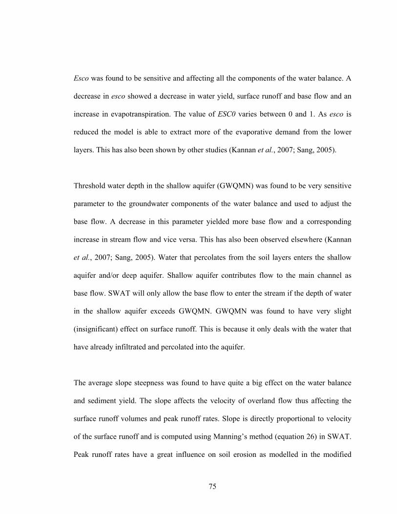
Esco was found to be sensitive and affecting all the components of the water balance. A

decrease in esco showed a decrease in water yield, surface runoff and base flow and an

increase in evapotranspiration. The value of ESC0 varies between 0 and 1. As esco is

reduced the model is able to extract more of the evaporative demand from the lower

layers. This has also been shown by other studies (Kannan et al., 2007; Sang, 2005).

Threshold water depth in the shallow aquifer (GWQMN) was found to be very sensitive

parameter to the groundwater components of the water balance and used to adjust the

base flow. A decrease in this parameter yielded more base flow and a corresponding

increase in stream flow and vice versa. This has also been observed elsewhere (Kannan

et al., 2007; Sang, 2005). Water that percolates from the soil layers enters the shallow

aquifer and/or deep aquifer. Shallow aquifer contributes flow to the main channel as

base flow. SWAT will only allow the base flow to enter the stream if the depth of water

in the shallow aquifer exceeds GWQMN. GWQMN was found to have very slight

(insignificant) effect on surface runoff. This is because it only deals with the water that

have already infiltrated and percolated into the aquifer.

The average slope steepness was found to have quite a big effect on the water balance

and sediment yield. The slope affects the velocity of overland flow thus affecting the

surface runoff volumes and peak runoff rates. Slope is directly proportional to velocity

of the surface runoff and is computed using Manning’s method (equation 26) in SWAT.

Peak runoff rates have a great influence on soil erosion as modelled in the modified

75

rational formula (equation 17) in SWAT. The average slope also affects the movement

of lateral flow. The average slope represent the topography of the sub-basin therefore

there is little adjustment that can be made about this parameter especially in areas where

the sub-basin has more or less uniform slope. On the hilly North Eastern part of the

watershed, a slight adjustment (within 10%) was done during the calibration.

Available soil water content (SOL_AWC) which is the difference between the Field

capacity of the soil and the wilting point was only adjusted within ± 0.004 m/m. This

component represents the soil storage and an increase would reduce all the other water

balance components. A comprehensive description of all the parameters is given in

Neistch et al. (2005)

4.3 Model Calibration

Figure 4.4 shows the calibration plot for stream flow. Monthly data was used for

calibration. The figure shows the ‘measured’ (generated from the reservoir) and

simulated stream flow in addition to mean monthly reservoir data for the same period.

The fit between the simulated and ‘measured’ flow hydrographs with an R2 of 0.6 was

found satisfactory under the existing conditions considering the water that was not

accounted for in the reservoir water balance which was used to generate the flow data.

The reservoir capacity when full is 16 million cubic meters of water.

76

As it can be seen the reservoir was full during the periods of April and July 1990 and

1993. This is during the rainy season (Figure 1.4). When the reservoir is full, the water

goes over the spillway. The flow over the spillway is not gauged at the reservoir. This

water was therefore not accounted for in the reservoir water balance which was used to

calculate the inflow into the reservoir. The reservoir inflow was used as the ‘measured’

stream flow in the calibration and validation of the model. During the rainy season when

the stream flow is high, the pipe from Kiburu sub-watershed can only carry a limited

capacity and so when full, the rest of the water goes downstream through Kiburu River

and thus do not go to the reservoir. The simulated flow would however include this

water. In 1991 and 1992, there is a relatively close agreement between the simulated and

the ‘measured’ stream flows. Although April-July is a rainy season, the reservoir was

not full during that period in 1991 and 1992 as shown in Figure 4.4. This means that no

or little water was lost through the spillway during that period. In November- December

of 1992, the reservoir was running full hence the reason we have relatively smaller peak

for simulated stream flow higher than the observed. There are also some cases where the

simulated flow was smaller than the observed flow this could be caused by the times

when the abstraction from the reservoir (outflow) was less than 64,000 m3 /day during

the dry seasons.

77

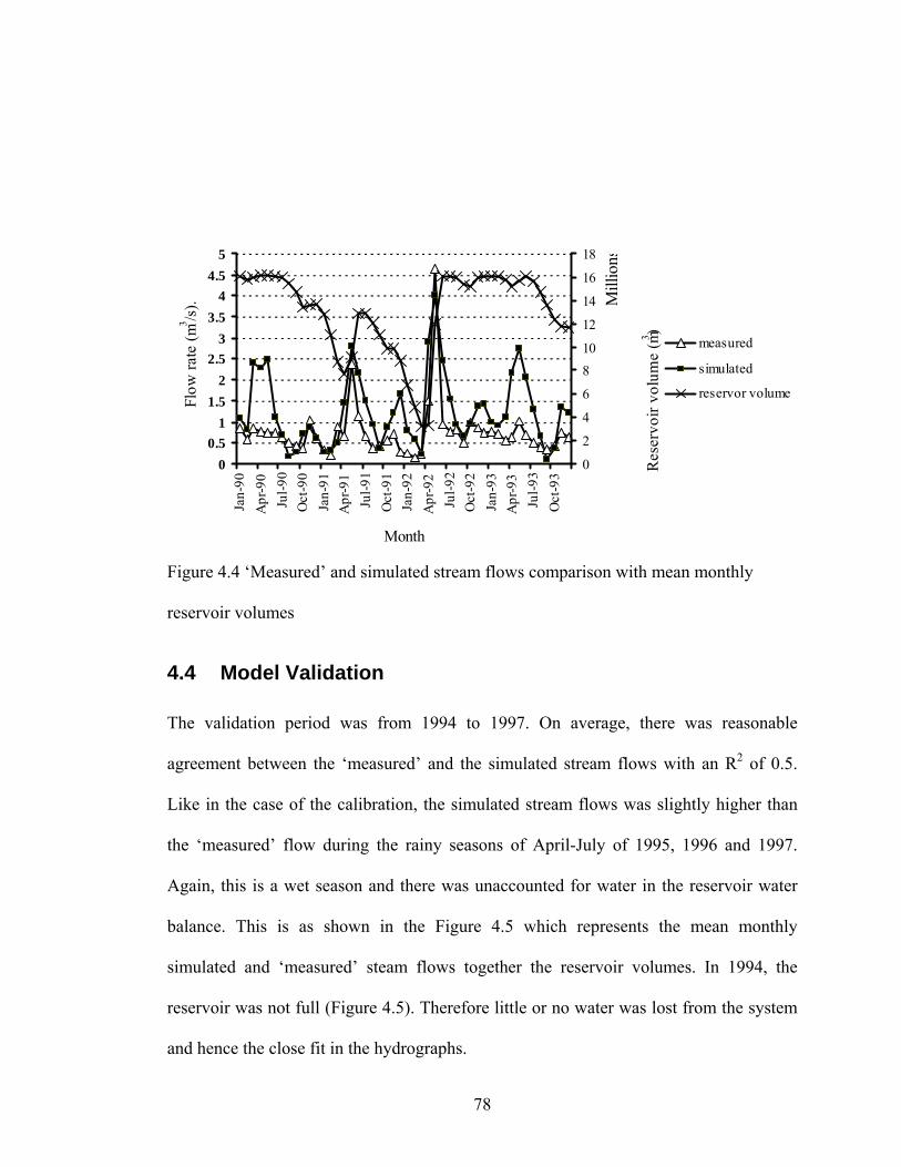
00.5

11.5

22.5

33.5

44.5

5Ja

n-90

Apr

-90

Jul-9

0O

ct-9

0Ja

n-91

Apr

-91

Jul-9

1O

ct-9

1Ja

n-92

Apr

-92

Jul-9

2O

ct-9

2Ja

n-93

Apr

-93

Jul-9

3O

ct-9

3Month

Flow

rate

(m3 /s

).

0

2

4

6

810

12

14

16

18

Mill

ions

Res

ervo

ir vo

lum

e (m3 )

measured

simulated

reservor volume

Figure 4.4 ‘Measured’ and simulated stream flows comparison with mean monthly

reservoir volumes

4.4 Model Validation

The validation period was from 1994 to 1997. On average, there was reasonable

agreement between the ‘measured’ and the simulated stream flows with an R2 of 0.5.

Like in the case of the calibration, the simulated stream flows was slightly higher than

the ‘measured’ flow during the rainy seasons of April-July of 1995, 1996 and 1997.

Again, this is a wet season and there was unaccounted for water in the reservoir water

balance. This is as shown in the Figure 4.5 which represents the mean monthly

simulated and ‘measured’ steam flows together the reservoir volumes. In 1994, the

reservoir was not full (Figure 4.5). Therefore little or no water was lost from the system

and hence the close fit in the hydrographs.

78

0

0.5

1

1.5

2

2.5

3

3.5

4

4.5

5

Jan-

94

Apr

-94

Jul-9

4

Oct

-94

Jan-

95

Apr

-95

Jul-9

5

Oct

-95

Jan-

96

Apr

-96

Jul-9

6

Oct

-96

Jan-

97

Apr

-97

Jul-9

7

Month

Flow

rate

s (m

3 /s)

0

2

4

6

8

10

12

14

16

18

Milli

ons

Res

ervo

ir vo

lum

e (m

3 )

measured

simulated

reservoir volume

Figure 4.5: Measured and simulated stream flow comparison with mean monthly

reservoir volumes

4.5 simulation of soil and water conservation practices

4.5.1 Vegetative filter strips

An increase in the width of the filter strip resulted in a decrease in the sediment loading

(Figure 4.6) with the first few meters having the greatest impact on reducing the loading

into the streams.

79

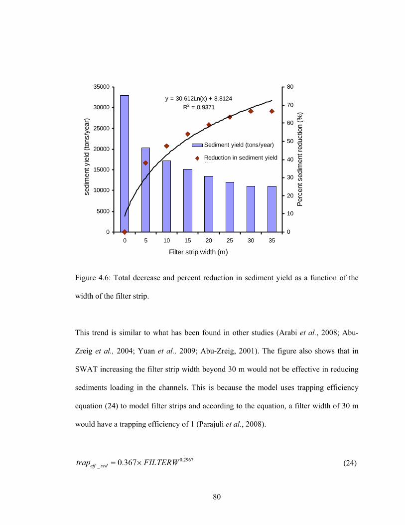
y = 30.612Ln(x) + 8.8124R2 = 0.9371

0

5000

10000

15000

20000

25000

30000

35000

0 5 10 15 20 25 30 35

Filter strip width (m)

sedi

men

t yie

ld (t

ons/

year

)

0

10

20

30

40

50

60

70

80

Per

cent

sed

imen

t red

uctio

n (%

)

Sediment yield (tons/year)

Reduction in sediment yield(%)

Figure 4.6: Total decrease and percent reduction in sediment yield as a function of the

width of the filter strip.

This trend is similar to what has been found in other studies (Arabi et al., 2008; Abu-

Zreig et al., 2004; Yuan et al., 2009; Abu-Zreig, 2001). The figure also shows that in

SWAT increasing the filter strip width beyond 30 m would not be effective in reducing

sediments loading in the channels. This is because the model uses trapping efficiency

equation (24) to model filter strips and according to the equation, a filter width of 30 m

would have a trapping efficiency of 1 (Parajuli et al., 2008).

2967.0_ 367.0 FILTERWtrap sedeff ×= (24)

80

Where trapeff_sed is trapping efficiency of the sediments and FILTERW is the width of the

filter strip (m).

In Sasumua, the small sizes of land (as small as a quarter of an acre) owned by many of

the small scale farmers can not allow large grass strips on the fields. Wolde and Thomas,

(1989), recommend installation of grass strips of 1.0 m to 1.5 m wide where land is not

scarce and 0.5 m where land is scarce in Kenya. This recommendation is valid for

contour grass strips and taking the advantage of the logarithmic relationship between the

sediment yield reduction and grass filter strip width. This relationship means that even

smaller widths of grass strips would still be beneficial in reducing soil loss. Wider filter

strips can be installed on the riparian areas where the government prohibits cultivation in

the agriculture act.

The logarithmic trend can be attributed to equation 24 which incorporates higher

efficiencies in the front portion of the strip in trapping the sediments (Arabi et al., 2008).

Yuan et al. (2009) after reviewing several studies on the effectiveness of the buffer strips

concludes that the trapping efficiency of the buffer width would be best fitted in a

logarithmic model and that a 5 m buffer can trap up to 80% of the sediments. Other

studies that have observed the similar results include; Robinson et al. (1996) who found

that the initial 3 m of vegetative filter strips removed more than 70% of the sediment,

Borin et al. (2005) found out that a 6 m buffer strip composed of trees and grass reduced

total suspended sediment load by about 78%, Ullrich and Volk, (2009) found out that a 2

81

m filter strip would result in a reduction of total sediment loading by about 45% when

simulated using SWAT. In Kenya, Ogweno, (2009) found that a 10m filter strip reduced

sediment yield by over 95% in Malewa watershed, in Naivasha Kenya.

The trapping efficiency of the filter strips depends on many factors but the width is the

major one (Abu-Zreig, 2001). Other factors include; vegetation type, density and

spacing, Manning’s roughness coefficient, flow concentration, soil type, sediment

particle size and the slope (Yuan et al., 2009; Abu-Zreig, 2001; Fox et al., 2010; White

and Arnold, 2009).

Buffers decrease the velocity of the surface runoff due to increased roughness provided

by the vegetation and in effect allow the sediments to settle due to the reduced sediment

transport capacity of the runoff. Buffers also enhance the infiltration of reducing the

amount of runoff thus aiding in sediment deposition also due to reduced sediment

transport capacity (Yuan et al., 2009; Borin et al., 2005; Abu-Zreig et al., 2004; White

and Arnold, 2009; Duchemin and Hogue, 2009).

In Sasumua, other than the reparian buffer strips at the reservoir and extending some

distance upstream of the feeding streams, very few farms have grass strips on their land.

Some farmers cultivate right into the streams banks and since some streams are seasonal,

they cultivate right into the channels when they are dry. Thus, Implementation of

vegetative strips in the whole watershed would ensure that the sediments are trapped and

retained on the land as opposed to the current state where they are washed into thee

82

streams. One of the ecosystem services that the watershed is expected to provide is

regulation/improvement of water quality. From the simulation results obtained here it is

quite clear then that vegetative filter strips would enhance this ecosystem service as far

as sedimentation is concerned.

Farmers in the watershed would have to compromise some of the crop land for

conservation if filter strips are to be implemented. This may not be easy due to the small

sizes of land that most of the farmers in the watershed have. For filters strips

implementation, the farmers need to be educated on the need for conservation and where

possible compensated for the land they would forgo for the purpose of the conservation.

Payment for Ecosystem Services (PES) should be evaluated for the watershed to find

ways of giving incentives to the farmers who do conservation and more so if they will

have to give up part of their land they use for crop production like in the case of filter

strips. The vegetation in the filter strip can also be selected to have multiple functions.

Other than NPS pollution abatement, filter strips comprising of trees and grass could

offer other benefits like timber production, carbon dioxide sequestration, aesthetics

(Borin et al., 2010), increasing the biodiversity of flora and fauna and providing habitat

for wildlife (Lovell and Sullivan, 2006). The grass can also be used as fodder for

livestock. In this way, the farmers will have a direct economic benefit from the trees and

the fodder and would be encouraged to preserve and maintain the filter strips for

pollution prevention purposes.

83

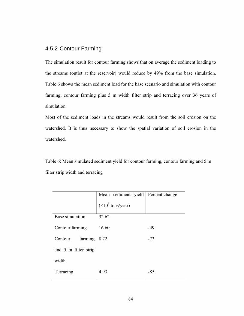
4.5.2 Contour Farming

The simulation result for contour farming shows that on average the sediment loading to

the streams (outlet at the reservoir) would reduce by 49% from the base simulation.

Table 6 shows the mean sediment load for the base scenario and simulation with contour

farming, contour farming plus 5 m width filter strip and terracing over 36 years of

simulation.

Most of the sediment loads in the streams would result from the soil erosion on the

watershed. It is thus necessary to show the spatial variation of soil erosion in the

watershed.

Table 6: Mean simulated sediment yield for contour farming, contour farming and 5 m

filter strip width and terracing

Mean sediment yield

(×103 tons/year)

Percent change

Base simulation 32.62

Contour farming 16.60 -49

Contour farming

and 5 m filter strip

width

8.72 -73

Terracing 4.93 -85

84

Figures 4.7 (a) and (b) shows spatial distribution of the annual sediment yield in ton/ha

from various sub-basins in the Sasumua sub-watershed before and after the

implementation of the contour farming respectively clipped from the entire Sasumua

watershed used in the simulation. The sediment yield values for the respective sub-

basins are shown in appendix 3. The base simulation results of sediment yield compares

well with that obtained by other studies in the area. Kigira, (2007) for example, found

that the sediment yield ranges between 2.0 -70 tons/ha/yr for the same location of the

watershed when he modelled the larger Thika watershed using SWAT model. Sasumua

River is a tributary of Chania River which is in turn a tributary of Thika River. Thus

Sasumua watershed is part of the larger Thika watershed. Other sediment studies that

have been done on the Chania watershed include; Dunne, (1974), who found that the

Chania watershed (522.4 km2) has a sediment yield of 0.19×106 tons/year, Ongwenyi,

(1978), 0.3×106 tons/year and Maingi, (1991) who found a sediment yield of 0.87×106

tons/year

Figure 4.7 (a) shows that sub-basins 9, 10, 11, 16, 18 and 61 which are under forest

cover have relatively low sediment yield. Low CN values were used, in equation 6, to

represent forest land cover in the model. Sub-basins 41, 42, 43, 47 and 60 were found to

have a relatively higher sediment yield. These are soil erosion hotspots which should be

prioritized when implementing soil conservation measures. This is in consistent with

earlier study by Gathenya et al. (2009). The main factors contributing to high sediment

yield in this part of the watershed is the low infiltration rates characteristic of planosols

85

(Fig. 1.2) which generates much runoff that cause more soil erosion. Sub-basins like 43

which are adjacent to the main streams also have higher averages slopes.

The results indicate that implementation of contour farming would reduce the soil

erosion in the farmlands. In general, contour farming can reduce soil erosion by 50%

compared to up and down cultivation (Mati, 2007). Other studies (Quinton and Catt,

2004; Arabi et al., 2008; Brunner et al., 2008) have also found that contour farming have

a positive effect in reducing sediment yield. For example, Quinton and Catt, (2004)

found out that on average over a period of 10 years experiment, across the slope plots

had a mean soil loss of 6.4 tons/ha compared the mean soil loss from the plots

cultivated up and down slope was 16.5 tons/ha. Gassman et al. (2006) found out that

contouring reduced sediment loss by 34% on average using 30 year simulation period by

SWAT model and by 53% by Agricultural Policy Environmental eXtender (APEX)

model over the same simulation period.

86

9

18

16

42

37

43

51

60

57

22

61

41

58

4438

48

10

30

17

36

24

11

29

52

12

20 15

21

47

19

35

23

59

1 0 1 2 3 Kilometers

Sediment yield (ton/ha)0 - 44 - 1010 - 1313 - 41

N

9

18

16

42

37

43

5160

57

22

61

41

58

4438

48

10

30

17

36

24

11

29

52

12

20 15

21

47

19

35

23

59

1 0 1 2 3 Kilometers

Sediment yied (ton/ha)0 - 11 - 44 - 77 - 19

N

Figure 4.7 (a): sediment yield for

base simulation

Figure 4.7 (b): sediment yield after

implementation of contour farming

Revised Universal Soil Loss Equation (RUSLE) simulation in Wangjiaqiao watershed in

China by Shi et al. (2004) found that contour tillage could reduce soil loss by 31%.

Contour farming is mainly associated with cultivation using agricultural machinery and

the contour farming parameter values found in literature would be more associated with

mechanized farming. In Sasumua however, most farmers practice hand hoe tillage.

There is minimal use of machinery tillage except when opening new land. Thus the

surface roughness that can be achieved by hand hoe tillage may not be equal to that of

87

machinery and therefore the sediment yield reduction may be lower than the values

simulated for this study.

Contour farming creates surface roughness blocking the surface runoff and encourages

infiltration as water pond in the depressions. This reduces the erosive power of surface

runoff and thus reduces soil erosion (Quinton and Catt, 2004; Arabi, et al., 2008).

From the water balance point of view, implementation of contour farming would result

in a decrease of surface runoff of 16% and an increase of base flow of 7.6% with only a

slight decrease in the total water yield (Table 7; Figure 4.8). In other studies, Quinton

and Catt, (2004) found out that event surface runoff from experimental runoff plots was

0.8 mm for cultivation across the slope compared to 1.32 mm when cultivation was done

up and down slope

The decrease in the surface runoff is a result of increased infiltration into the ground of

water. Contour farming would cause impounding of water into the small depressions and

thus more water would infiltrate into the ground (Quinton and Catt, 2004). This would in

effect enhance the recharge of the shallow aquifer and water will be released to the

streams as base flow.

88

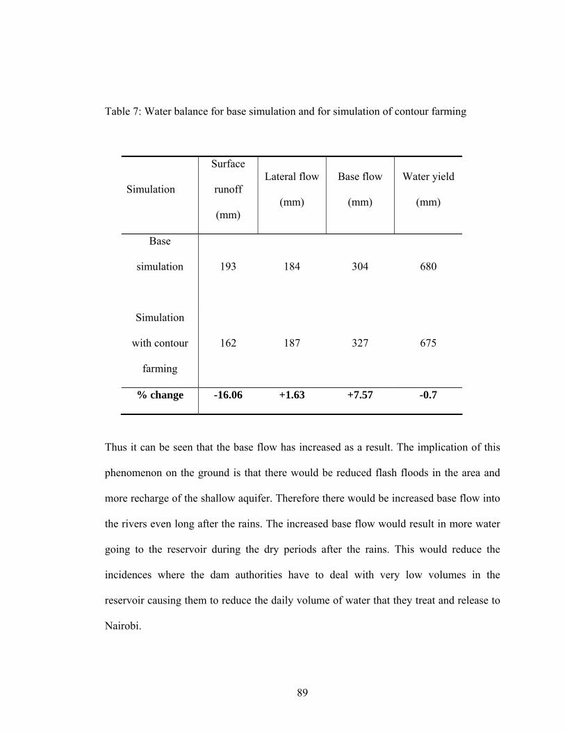
Table 7: Water balance for base simulation and for simulation of contour farming

Simulation

Surface

runoff

(mm)

Lateral flow

(mm)

Base flow

(mm)

Water yield

(mm)

Base

simulation

193 184 304 680

Simulation

with contour

farming

162 187 327 675

% change -16.06 +1.63 +7.57 -0.7

Thus it can be seen that the base flow has increased as a result. The implication of this

phenomenon on the ground is that there would be reduced flash floods in the area and

more recharge of the shallow aquifer. Therefore there would be increased base flow into

the rivers even long after the rains. The increased base flow would result in more water

going to the reservoir during the dry periods after the rains. This would reduce the

incidences where the dam authorities have to deal with very low volumes in the

reservoir causing them to reduce the daily volume of water that they treat and release to

Nairobi.

89

The results here show that implementation of contour farming would improve water

quality and regulate flows i.e. increase dry weather flows and reduce flash floods. Thus

contour farming would improve the capacity of the watershed to provide the two

regulatory ecosystem services (water quality improvement and flow regulation).

4.5.3 Contour farming and filter strips

Results for the simulation of a combination of filter strip and the contour farming

implemented in the watershed would have a significant reduction in the sediment

loading to the streams. A combination of contour farming and 5 metre wide filter strip

would result in 73 % reduction in sediment loading from the base simulation (Table 6).

Contour farming would reduce soil erosion in the farms and the filter strips would trap

the eroded soil before it gets to the streams.

Implementing contour farming together with grass filter strips would be more beneficial

than implementing either of the conservation practice on its own. Contour farming is an

insitu soil conservation method and would ensure minimum soil displacement and

minimum loss of soil fertility. On the other hand the filter strips will trap sediments that

have been eroded and carried by the runoff before they get to the streams thus ensuring

good water quality. This would also reduce the sedimentation of the reservoir which

would offer some benefits to the dam management authorities. There would be less loss

of reservoir storage capacity from siltation. The reduced sedimentation would offer a

90

direct benefit in reduction of the water treatment costs associated with the turbidity.

Aluminum sulphate (alum) is used for coagulation and flocculation of the suspended

particles in the water treatment process. More of this chemical is used during the rainy

season when the water contains more sediments. Thus reduction in the sedimentation of

the streams and subsequent siltation of the reservoir would result in the reduction of

water treatment cost.

4.5.4 Terracing

The results of sediment loading into the streams and the reservoir from Sasumua sub-

watershed show that terracing would reduce the sediment loading by 85% (Table 6).

Implementation of bench terraces in the watershed would reduce the sediment loading to

the reservoir. Less sediment into the reservoir will reduce the cost of treatment of water

due to turbidity and also reduce the loss of capacity of the reservoir due to siltation.

These results compares well with other studies on the effectiveness of terraces in

reducing sediment yield. Gassman et al. (2006) found out that terraces would reduce

sediment yield by about 63.9 % and 91.8% using SWAT and APEX models simulations

respectively. Santhi et al. (2006) found that contour terraces would reduce sediment

yield by between 84 and 86% using SWAT simulations at the farm level.

Terraces enhance the ponding of water on the surface hence allowing higher rates of

infiltration. The velocity of the remaining surface runoff would be reduced and thus the

91

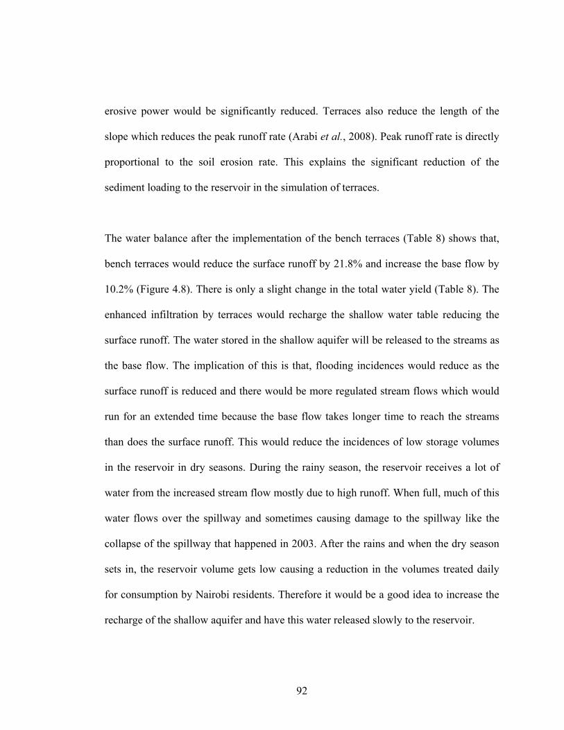
erosive power would be significantly reduced. Terraces also reduce the length of the

slope which reduces the peak runoff rate (Arabi et al., 2008). Peak runoff rate is directly

proportional to the soil erosion rate. This explains the significant reduction of the

sediment loading to the reservoir in the simulation of terraces.

The water balance after the implementation of the bench terraces (Table 8) shows that,

bench terraces would reduce the surface runoff by 21.8% and increase the base flow by

10.2% (Figure 4.8). There is only a slight change in the total water yield (Table 8). The

enhanced infiltration by terraces would recharge the shallow water table reducing the

surface runoff. The water stored in the shallow aquifer will be released to the streams as

the base flow. The implication of this is that, flooding incidences would reduce as the

surface runoff is reduced and there would be more regulated stream flows which would

run for an extended time because the base flow takes longer time to reach the streams

than does the surface runoff. This would reduce the incidences of low storage volumes

in the reservoir in dry seasons. During the rainy season, the reservoir receives a lot of

water from the increased stream flow mostly due to high runoff. When full, much of this

water flows over the spillway and sometimes causing damage to the spillway like the

collapse of the spillway that happened in 2003. After the rains and when the dry season

sets in, the reservoir volume gets low causing a reduction in the volumes treated daily

for consumption by Nairobi residents. Therefore it would be a good idea to increase the

recharge of the shallow aquifer and have this water released slowly to the reservoir.

92

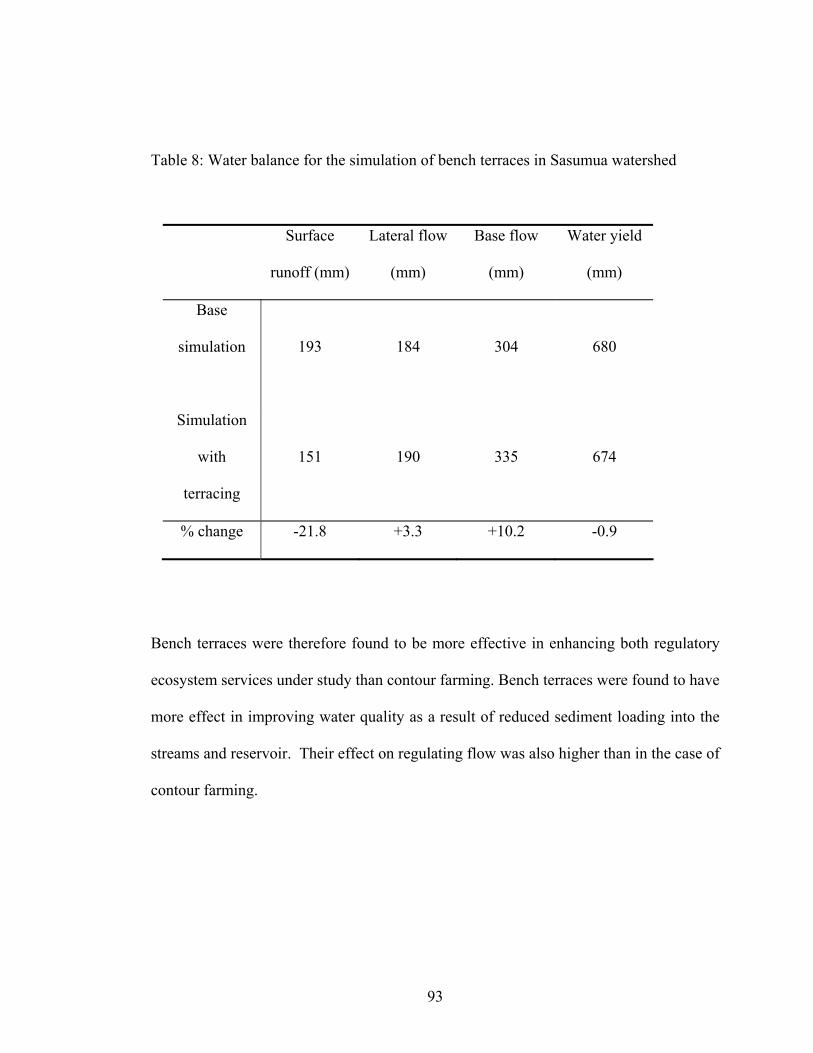
Table 8: Water balance for the simulation of bench terraces in Sasumua watershed

Surface

runoff (mm)

Lateral flow

(mm)

Base flow

(mm)

Water yield

(mm)

Base

simulation

193 184 304 680

Simulation

with

terracing

151 190 335 674

% change -21.8 +3.3 +10.2 -0.9

Bench terraces were therefore found to be more effective in enhancing both regulatory

ecosystem services under study than contour farming. Bench terraces were found to have

more effect in improving water quality as a result of reduced sediment loading into the

streams and reservoir. Their effect on regulating flow was also higher than in the case of

contour farming.

93

0

100

200

300

400

500

600

700

800

Base scenario contour farming Bench terrace

Wat

er (m

m)

Surface runoffLateral flowBase flow

Figure 4.8: Effect of contour farming and Bench terraces on water balance components

4.5.5 Grassed waterway

The results from the simulation of the grassed waterway (Table 9) show that, they would

have a sediment reduction of 40.72% when simulated at the outlet of Mingotio stream at

the reservoir (sub-basin 60) and 23.45% for the whole Sasumua sub-watershed

(simulated at the outlet of sub-basin 61). There was only a very slight change in the

stream flow.

94

This shows that grassed waterways can play a great role in the reduction of sediments in

Sasumua. Other studies that have found similar results on the reduction of sediment

yield by grassed waterways include; Fiener and Auerswald, (2006a) who found a

sediment reduction of about 93% for a 290 m long and 37 m wide grassed waterway.

Table 9: Simulated sediment yield and stream flow reduction with and without grassed

waterway.

Sediment Yield (× 103 tons/year) Streamflow (m3/s)

Outlet at

Mingotio

stream (sub-

basin 60)

Main Sasumua

sub-watershed

outlet (at sub-

basin 61)

Outlet at

Mingotio

stream (sub-

basin 60)

Main Sasumua

sub-watershed

outlet (at sub-

basin 61)

Without GWW 20.60 32.75 0.603 1.483

With GWW 12.21 25.07 0.601 1.481

% change 40.72 23.45

Implementation of grassed waterway takes a relatively big land and is usually not much

practiced in Kenya where the land sizes are small to the extent of quarter an acre in some

areas. However, in Sasumua grassed waterway would be of much importance as a way

95

of reducing the sediments that are usually washed from the cultivated lands near the

seasonal streams/channels during the rainy season.

This is because the farmers cultivate so close to the channels which are usually dry

during the dry season and when the rains come the sediments and sometimes crops from

these lands are washed by the increased water in the channels/streams.

The increased roughness of the channels has a great effect in the reduction of the

sediment yield. The grass would reduce the velocity of the water in the waterway and in

effect reduce the stream power and its sediment transporting capacity hence causing

deposition (Simon and Rinaldi, 2006). In SWAT sediment routing, the maximum

sediment that can be transported is modeled as a function of the peak channel velocity

(V cm/s) calculated as (Neitsch et al., 2005);

Aq pkV = (25)

Where, A is the cross sectional area of flow in the channel segment (m2) and qpk is the

channel peak flow rate (m3/s) adjusted by a factor from the average rate of flow, q

calculated as shown in equation 26;

nSRAq 2/13/2.= (26)

96

Where; R is the hydraulic radius for the depth of flow (m), S is the slope of the channel

segment (m/m) and n is the Manning’s coefficient for the channel section which is the

parameter CH_N2 adjusted in the model. The maximum sediment that can be

transported from a reach segment is then calculated as;

expspspsed vcConc ×= (27)

Where concsed is the maximum concentration of sediment that can be transported by

water (tons/m3), Csp is a coefficient defined by the user and spexp is an exponent defined

by the user (between 1.0 and 2.0). Deposition of the sediment in the reach occurs if the

sediment in the water is more than the maximum concentration of sediment that can be

transported by the water in that part of the reach.

From equation 27, it is evident that the reduction in velocity of water in the channel

would reduce the maximum sediment that can be transported by the water and if the

sediment in the reach is more than that capacity then the excess sediments will be

deposited in the channel. It is worth emphasizing that the values adopted for the

Manning’s channel roughness is for dense grasses under non sub-merged condition, if

the grasses bend, break or get submerged, the value would drop (Fiener and Auerswald,

2006a). Thus, the effectiveness of this conservation practice in Sasumua would largely

depend on the maintenance of the waterway.

97

4.5.6 Additional management scenarios

A comparison of alternative land management practices in the agricultural part of the

watershed shows that sediment loading to the streams would increase by 53.6% for the

poor land management scenario (intensive cultivation and overgrazing) and reduce by

34.3% in the case of good land management scenario (less intensive cultivation and well

managed grazing), both in reference to the base simulation. Table (10) shows the

sediment loading and the water yield for the two scenarios simulated for 36 years.

An increase in CN resulted in an increase in the sediment load (Table 10). Continued

poor management of the agricultural land in Sasumua would result in reduction in

infiltration of rain water into the ground. This would result in an increase in the peak

runoff rates and thus more soil erosion. A reduction in CN resulted in a decrease in

sediment loading. This is because of the improved infiltration conditions which were

modeled by reducing the CN. The increased infiltration would result in a decrease in the

surface runoff rates and thus less soil erosion.

Good land management will result in an increase in the infiltration of the rain water and

a result a reduction in the surface runoff and an increase in the base flow. The good land

management scenario, which was simulated by decreasing the CN by 6 units from the

base simulation, resulted in a 28.5 % decrease in surface runoff, a 13.8% increase in

base flow and a slight decrease in total water yield of 1.2% (Table 10).

98

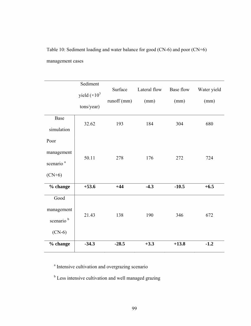
Table 10: Sediment loading and water balance for good (CN-6) and poor (CN+6)

management cases

Sediment

yield (×103

tons/year)

Surface

runoff (mm)

Lateral flow

(mm)

Base flow

(mm)

Water yield

(mm)

Base

simulation 32.62 193 184 304 680

Poor

management

scenario a

(CN+6)

50.11 278 176 272 724

% change +53.6 +44 -4.3 -10.5 +6.5

Good

management

scenario b

(CN-6)

21.43 138 190 346 672

% change -34.3 -28.5 +3.3 +13.8 -1.2

a Intensive cultivation and overgrazing scenario

b Less intensive cultivation and well managed grazing

99

On the other hand, a poor management scenario would lead poor infiltration of rain

water into the ground thus increasing the surface runoff and decreasing the base flow.

This scenario which was simulated by an increase in the CN by 6 units from the base

simulation resulted in an increase in surface runoff by about 44 %, a 10.5 % reduction in

base flow and 6.5% increase in water yield.

100

CHAPTER 5

CONCLUSIONS AND RECOMMEDATIONS

5.1 Conclusions

Sasumua watershed currently is limited to produce some of environmental services it is

expected to produce mainly because of human activities. In particular, the watershed is

limited in offering two environmental services namely improvement of water quality and

regulation of stream flows. Poor land management activities currently being practiced

such as over-cultivation and overgrazing have increased sediment loading to the streams

and the reservoir thus impairing water quality and also reducing infiltration of water into

the ground. This has resulted in flash flood during the rainy seasons and low dry weather

flows. This study has however found that the two environmental services would be

enhanced if soil and water conservation measures are implemented in the watershed.

The study obtained that the grass filter strips reduce sediment yield as a function of their

width. The first few increments of 5 m intervals had more reduction in sediment yield.

This implies that even narrower strips would be relatively effective in trapping the

sediments. This is attributed to the trapping efficiency that SWAT uses to model

sediment yield in the filter strips which places a higher efficiency in the front part of the

filter strip in trapping sediments. Simulation of contour farming was found to reduce

sediment yield by about 49%. A combination of 5 meter filter strips and contour farming

101

would have a sediment reduction of 73%. Installation of bench terraces would result in

about 85% reduction in sediment load. Both the contour farming and bench terraces

reduced surface runoff and increased base flow with only minimal decrease in total

water yield. Reduced surface runoff will reduce incidences of flash floods while

increased base flows will ensure increased dry weather flows. Bench terraces were the

most effective soil conservation practice in reducing sediment yield as well as increasing

water infiltration.

If implemented in four sub-basins that have a drainage ditch, grassed waterway would

result in a 41% decrease in the sediment load in the outlet of Mingotio stream and a 23%

reduction for the entire Sasumua sub-watershed. There was no significant change in the

steam flow in the simulation of grassed waterway.

Improved land management methods would reduce sediment yield by 34% and surface

runoff by 28.5%. It would increase the base flow by 14%. Poor land management would

increase sediment yield by 53.6% surface runoff by 44% and reduce the base flow by

10.5%.

In summary, implementation of soil and water conservation practices in Sasumua

watershed would enhance its capacity to provide some key ecosystem services i.e. water

quality improvement and flow regulation. Soil and Water conservation practices would

reduce the incidences and magnitudes of flash floods and slightly increase the dry

102

weather flows. It would also reduce the soil erosion from the farmland and therefore

reducing the loss of soil fertility and subsequently reduce the sediments washed into the

streams as well as the siltation of the reservoir.

5.2 Recommendations

Soil erosion ‘hotspots’ were identified, and I recommend that these areas should be

prioritized in the implementation of soil and water conservation measures.

Implementation of soil conservation measures in these areas would reduce soil erosion

and reduce the sedimentation into the streams and the reservoir thus boosting the

capacity of the watershed to produce the environmental service of improving the water

quality.

Bench terraces were found to be the most effective conservation practice in reducing

sediment yield and increasing infiltration. It is recommended that bench terraces should

be constructed in the watershed. However, terraces are structural conservation practices

and involve some earth work during their implementation and therefore relatively

expensive. For farmers who can meet the cost, I recommend that they should directly

construct the terraces especially in the erosion hotspots identified. For those who may

not be able to meet the cost, I recommend that they install grass strip which will

eventually evolve into bench terraces.

103

I further recommend construction of grassed waterway in the drainage channels that feed

water to Mingotio stream.

Further research should be conducted to identify the willingness of the farmers to invest

in soil and water conservation. The research should also identify what conservation

practices are the farmers more willing to embrace. A Payment for Ecosystem Services

(PES) scheme should also be evaluated whether it can work in the watershed. A PES

scheme identifies buyers (beneficiaries) and sellers (stewards) of ecosystem services and

assesses the willingness of the buyers to give incentives to the sellers to engage in

activities that enhance the environmental services.

Stream flow data for the gauging stations in the watershed was not available since it is

not collected. Hydrological projects and studies like hydrological modelling rely on

these data. Availability of that data would improve the calibration and validation of the

model. The ministry of water through Water Resources Management Authority should

put mechanisms of collecting the data.

Water balance in the reservoir has also been shown as a method that can be used for the

calibration and validation of the model. To improve the calibration exercise the NWSC

should keep better records of water abstraction from the reservoir and also have a gauge

104

at the spillway. Daily recorded data would improve the calibration and validation of the

model as compared to the monthly approach used.

105

REFERENCES

Abu-Zreig M., 2001. Factors affecting sediment trapping in vegetated filter strips:

simulation study using VFSMOD. Hydrological. Processes. 15,

1477–1488

Abu-Zreig M, R. P. Rudra, M. N. Lalonde, H. R. Whiteley and N. K. Kaushik,

2004. Experimental investigation of runoff reduction and sediment

removal by vegetated filter strips. Hydrological Processes 18: 2029–

2037.

Allen R.G., L.S.Pereira, D.Raes and M. Smith, 1998. Crop evapotranspiration:

Guidelines for computing crop water requirements - FAO Irrigation

and drainage paper 56. FAO - Food and Agriculture Organization of

the United Nations Rome, 1998.

http://www.fao.org/docrep/X0490E/x0490e00.htm#Contents,

accessed 15th April 2010.

Arabi, M., J. Frankenberger, B. Engel, and J. Arnold. 2008. Representation of

agricultural management practices with SWAT. Hydrol. Process.

Wiley interscience.

Arabi M., R. S. Govindaraju, M. M. Hantush, 2007. A probabilistic approach for

analysis of uncertainty in the evaluation of watershed management

practices. Journal of Hydrology (2007) 333, 459– 471

106

Bhattarai S., 2009. Spatially explicit assessment of tradeoffs and synergies amongst key

ecosystem services in Sasumua watershed, Kenya. Masters thesis.

School of Environment, Natural Resources and Geography. Bangor

University, Bangor, United Kingdom.

Biamah E.K., K. Fahlstrom, C.K.K. Gachene, J.M. Gachingiri, J.K. Kiara, M.

Mbegera, P. Mbogo, C.N. Mburu, K. Mutunga, F.S. Muya and

D.B. Thomas, 1997. Soil and Water Conservation manual for Kenya.

Eds. D.B. Thomas, A. Eriksson, M. Grunder and J.K. Mburu. Soil and

water conservation Branch, Ministry of agriculture, livestock

Development and marketing, Nairobi, Kenya.

Borin M, M.Vianello, F. Morari and G. Zanin, 2005. Effectiveness of buffer strips in

removing pollutants in runoff from a cultivated field in North-East

Italy. Agriculture, Ecosystems and Environment 105: 101–114.

Elsevier B.V.

Borin M., M. Passoni, M. Thiene and T. Tempesta, 2010. Multiple functions of

buffer strips in farming areas. Europ. J. Agronomy 32: 103–111.

Bracmort, K. S., M. Arabi, J. R. Frankenberger, B. A. Engel, and J. G. Arnold.

2006. Modeling long‐term water quality impact of structural BMPs.

Trans. ASABE 49 (2): 367‐374.

Brunner A.C., S.J. Park, G.R. Ruecker and P.L.G. Vlek, 2008. Erosion modeling

approach to simulate the effect of land management options on soil

107

loss by considering Catenary soil development and farmers

perception. Land degradation & development, 19: 623–635

Chi H., 2000. Computer simulations model for sustainability. International journal of

Sustainability in higher education, 1 (2): 154-167

Duchemin M. and R. Hogue, 2009. Reduction in agricultural non-point source

pollution in the first year following establishment of an integrated

grass/tree filter strip system in southern Quebec (Canada).

Agriculture, Ecosystems and Environment 131: 85–97

Dunne T., 1974. Suspended sediment data for Rivers of Kenya. Washington D.C.

Evrard O., K. Vandaele, B. van Wesemael and C. L. Bielders 2008. A grassed

waterway and earthen dams to control muddy floods from a cultivated

catchment of the Belgian loess belt. Geomorphology 100: 419–428

FAO (Food and Agriculture Organizaion), 1997. The digital Soil and Terrain

Database of East Africa. Notes on the Arc Info files. Version 1.

FAO (Food and Agriculture Organizaion), 2001. Lecture notes on the major soils of

the world: World soil resources report-94,

http://www.fao.org/docrep/003/Y1899E/y1899e12.htm, accessed,

22nd April 2010.

Fiener P., K. Auerswald, 2005. Measurement and modeling of concentrated runoff in

grassed waterways. Journal of Hydrology 301:198–215

108

Fiener P and K. Auerswald 2006a. Seasonal variation of grassed waterway

effectiveness in reducing runoff and sediment delivery from

agricultural watersheds in temperate Europe. Soil & Tillage Research

(87): 48–58

Fiener P and K. Auerswald 2006b. Influence of scale and land use pattern on the

efficacy of grassed waterways to control runoff. Ecological

engineering (27): 208–218.

Fox G.A. R. Munoz-Carpena and G.J. Sabbagh, 2010. Influence of Flow

Concentration on Parameter Importance and Prediction Uncertainty

for Vegetative Filter Strips. Journal of Hydrology (2010),

doi:10.1016/j.jhydrol.2010.01.020

Gassman P.W., E. Osei, A. Saleh, and J. Rodecap, 2006. Alternative practices for

sediment and nutrient loss control on livestock farms in northeast

Iowa. Agriculture, Ecosystems and Environment 117:135–144

Gassman P.W., M.R. Reyes, C.H.Green and J.G. Arnold, 2007. The Soil and Water

Assessment Tool: Historical Developments, Applications and Future

Research Directions. Transactions of ASABE, 50 (4): 1211-1250.

Galvan L., Olias M., Fernadez de Villaran R., Domingo Santos J.M., Nieto J.M,

Sarmieto A. M. And Canovas C.R., 2009. Application of SWAT

model to an AMD-affected river (Meca River, SW Spain). Estimation

of transported pollutant load. Journal of hydrology 377 (2009) 445-

454.

109

Gathenya J.M, Thiong’o G.T., and Mwangi J.K 2009. Hydrologic and water quality

assessment report for Sasumua watershed. Technical report. Word

agroforesty Centre. Unpublished report.

Gilley J.E., B. Enghball, L.A. Kramer and T.B. Moorman, 2000. Narrow grass hedge

effects on runoff and soil loss. Journal of soil and water conservation.

55 (2): 190-196.

Hudson N. 1989. Soil Conservation. B T Batsford Limited, London.

Iftikhar U.A, Kallesoe M, Duraiappah A, Sriskanthan G, Poats SV and Swallow B.

2007. Exploring the inter-linkages among and between Compensation

and Rewards for Ecosystem Services (CRES) and human well-being:

CES Scoping Study Issue Paper no. 1. ICRAF Working Paper no. 36.

Nairobi: World Agroforestry Centre.

Kannan N., S.M. White, F. Worrall and M.J. Whelan, 2007. Sensitivity analysis and

identification of best Evapotranspiration and runoff options for

hydrological modeling in SWAT 2000. Journal of hydrology (2007),

332, 456-466.

Kamar M.J., 1998. Soil Conservation approaches in Kenya. Advances in GeoEcology

31, 1057-1064. In Towards sustainable land use: Furthering

cooperation between people and institutions Volume II. Eds. Bume

H.P., H.E. Fleischhauer, A. Hebel, K.G. Steiner. Catena Verlag

GMBH, Reiskirchen, Germany.

110

Kigira F.K., 2007. Modelling the influence of land use changes on water and sediment

yield in the Thika River catchment using SWAT model. Master of

Science Thesis. Jomo Kenyatta University of Agriculture and

Technology.

Kinnell P.I.A. 2010. Event soil loss, runoff and the Universal Soil Loss Equation family

of models. A review. Journal of hydrology, doi:

10.1016/j.jhydrol.2010.01.024.

Liniger H.P., D. Cahill, W. Critchley, D. Thomas, G.W.J. van Lynden and G.

Schwilch, 2002. Categorization of soil and water technologies and

approaches- A global need? 12th ISCO conference, Beijing, china.

Lovell S.T and W. C. Sullivan, 2006. Environmental benefits of conservation buffers in

the United States:Evidence, promise, and open questions. Agriculture,

Ecosystems and Environment 112:249–260

Maingi S.M. 1991. Sedimentation in Masinga Reservoir. Msc. thesis, Kenyatta

University.

Mati B.M. 2007. 100 ways to manage water for smallholder agriculture in East and

Southern Africa. A compendium of technologies and practices.

SWMnet working paper 13. IMAWESA.

Mati B.M., 2006 Overview of water and soil nutrient management under small holder

rain-fed agriculture in East Africa. International Water Management

Institute (IWMI) working paper no. 105.

111

Millennium Ecosystem Assessment (MA). 2003. Ecosystems and Human Wellbeing: A

Framework for Assessment. Washington, DC: Island Press.

http://www.millenniumassessment.org/en/Framework.aspx

Mireri C., 2009. Preliminary Environmental Audit for Sasumua watershed. Technical

report. Word agroforesty Centre. Unpublished report.

Morgan R.P.C, 1986. Soil erosion and conservation. Longman Group limited.

Morgan R.P.C, 1980. Topics in applied geography: Soil erosion. Longman Group

limited.

Munoz-Carpena R, J.E. Parsons and G.J. Wendell, 1999. Modeling hydrology and

sediment transport in vegetative filter strips. Journal of Hydrology

214: 111–129.

Nash J E and J.V. Sutcliffe, 1970. River flow forecasting through conceptual models:

Part I. A discussion of principles. Journal of Hydrology, 10: 282–290

Natural Resource Conservation Service (NRCS), 1997. Contour Buffer Strips.

Conservation practice job sheet 332.

Natural Resource Conservation Service (NRCS), 2006. Contour farming:

Conservation practice Job sheet: PA330

Natural Resource Conservation Service (NRCS), 2009. Natural resources

Conservation Services: Natural resources conservation practice

standard: Terraces- code 600.

112

Ndomba P., F. Mtalo and A. Killingtveit, 2008. SWAT model application in a data

scarce tropical complex catchment in Tanzania. Physics and

Chemistry of the Earth 33 (2008) 626–632, Elsevier B.V.

Neitsch, S.L., Arnold, J.G., Williams, J.R., Kiniry, and K.W.King, 2002. Soil and

Water Assessment Tool (Version 2000) Model Documentation.

GSRWRL02-01, BREC 02-05, TR-191, Texas Water Research

Institute, Texas A&M University, College Station, TX. Available at:

http://www.brc.tamus.edu/swat.

Neitsch, S.L., Arnold, J.R., Kiniry and J.G. Williams 2005. Soil and Water

Assessment Tool (Version 2005) Model Documentation. Temple

Tex.: USDA-ARS Grassland, Soil and water research laboratory.

Available at: http://www.brc.tamus.edu/swat/doc.html

Ogweno L.P., 2009. Hydrologic analysis of Malewa watershed as a basis for

implementing Payment for Environmental Services (PES). Master of

Science thesis, Biomechanical and Environmental Egineering

Department, Jomo Kenyatta University of Agriculture and

Technology.

Ongwenyi G.S. 1978. Erosion and sediment transport in the upper Tana catchment with

special reference to the Thiba Basin. PhD thesis, University of

Nairobi.

113

Parajuli P.B., K.R. Mankin and P.L. Barnes, 2008. Applicability of targeting

vegetative filter strips to abate fecal bacteria and sediment yield using

SWAT. Agricultural water management, 95: 1189 – 1200.

Quinton J.N. and J.A. Catt, 2004. The effects of minimal tillage and contour

cultivation on surface runoff, soil loss and crop yield in the long-term

Woburn Erosion Reference Experiment on sandy soil at Woburn,

England. Soil Use and Management, 20: 343–349

Refsgaard J.C. 1996. Terminology, modellig protocol and classification hydrological

model codes. In Abbott M.B., B. Michael, J.C. Refsgaard and J.

Christian (eds) Distributed hydrological modeling. Kluwer academic

publishers, Netherlands. 17-40

Renard, K.G., G.R. Foster, G.A. Weesies, D.K. McCool and D.C. Yoder, 1997.

Predicting soil erosion by water: A guide to conservation planning

with the Revised Universal Soil Loss Equation (RUSLE). U.S.

Department of Agriculture Agricultural Handbook. No. 703. US

Department of Agriculture, Washington, DC

Robinson C.A., M. Ghaffarzardah, and R.M. Cruse 1996. vegetative filter strip effect

on sediment concentration in cropland runoff. Journal of soil and

water conservation 50 (3): 220-223

114

Sahu M. and R.R. Gu, 2009. Modelling the effects of the riparian buffer Zone and

contour strips on stream water quality. Ecological Engineering 35

(2009) 1167-1177, Elsevier B.V.

Sang J. K., 2005. Modelling the impact of changes in land use, climate and reservoir

storage on flooding in the Nyando basin. Masters thesis submitted to

Biomechanical and Environmental Engineering Department, Jomo

Kenyatta University of Agriculture and Technology, Kenya.

Santhi, C., R. Srinivasan, J. G. Arnold, and J. R. Williams. 2006. A modeling

approach to evaluate the impacts of water quality management plans

implemented in a watershed in Texas. Environ. Model. Soft. 21(8):

1141‐1157.

Shi Z.H., C.F. Cai, S.W. Ding, T.W. Wang and T.L. Chow, 2004. Soil conservation

planning at the small watershed level using RUSLE with GIS: a case

study in the Three Gorge Area of China. Catena 55:33–48

Singh V.P. and D.F. Frevert 2002. Mathematical modeling of watershed hydrology. In

Singh V.P. and D.F. Frevert (eds): Mathematical models for large

watershed hydrology. Water resources publications LLC Colorado,

USA.

Simon A. and M. Rinaldi, 2006. Disturbance, stream incision, and channel evolution:

The roles of excess transport capacity and boundary materials in

controlling channel response. Geomorphology 79: 361–383

115

Stevens C.J., J.N. Quinton, A.P. Bailey, C. Deasy, M. Silgram and D.R. Jackson,

2009. The effects of minimal tillage, contour cultivation and in-field

vegetative barriers on soil erosion and phosphorus loss. Soil & Tillage

Research 106: 145–151

Swallow B. M., J.K. Sang, M. Nyabenge, D.K. Bundotich, A.K. Duraiappah and

T.B. Yatich 2009. Tradeoffs, Synergies and traps among ecosystem

services in Lake Victoria basin of East Africa. Environmental science

and policy 12 (2009) 504-519. Elsevier Ltd.

Ullrich A. and M. Volk, 2009. Application of the Soil and Water Assessment Tool

(SWAT) to predict the impact of alternative practices on water quality

and quantity. Agricultural Water Management 96 (2009) 1207-1217,

Elsevier B.V.

USDA-NRCS, 2008. Natural Resource Conservation Practice standard: Filter strips.

Available online at:

http://www.nrcs.usda.gov/technical/Standards/nhcp.html

Van Lynden G.W.J. and H. Liniger 2002. WOCAT: a standard methodology of

documenting and evaluating soil and water conservation. Proceedings

of the Asian regional workshop on watershed management.

Vorosmarty C. J., C. Leveque, C. Revenga R. Bos, C. Caudill, J. Chilton, E. M.

Douglas, M. Meybeck, D. Prager P. Balvanera, S. Barker, M.

116

Maas, C. Nilsson, T. Oki, C.A. Reidy, 2003. Fresh water. In

Ecosystems and Human Well-being: Current State and Trends. Island

press. 167-201 pp

Vagen T.G., 2009. Asssessment of land degradation in Sasumua watershed. Baseline

report. Technical report. Word agroforesty Centre. Unpublished

report.

White M.J. and J. G. Arnold, 2009. Development of a simplistic vegetative filter strip

model for sediment and nutrient retention at the field scale.

Hydrological. Processes. 23, 1602–1616

Williams J.R., 1969. Flood routing with variable travel time or variable storage

coefficients. Transactions of the ASAE 12(1): 100-103

Williams J.R. 1975. Sediment routing for agricultural watersheds. Journal of the

American Water Resources Association, Paper No. 75065 of the

Water Resources Bulletin.

Wischmeier W. H. and Smith, D.D. 1978. Predicting rainfall erosion losses- a guide to

conservation planning. U.S. department of Agriculture, Agriculture

handbook no. 537.

Wolde F.T. and D.B. Thomas, 1989. The effect of narrow grass strips in reducing soil

loss and runoff on a Kabete Nitisol, Kenya. In Soil and water

conservation in Kenya. Proceedings of the third National workshop.

Kabete, Nairobi 16-19th September, 1986. Department of Agricultural

Engineering, University of Nairobi.

117

Yang Q, F-R Meng, Z. Zhao, T. L. Chow, G. Benoy, H. W. Rees, C. P.-A. Bourque,

2009. Assessing the impacts of flow diversion terraces on stream

water and sediment yields at a watershed level using SWAT model.

Agriculture, Ecosystems and Environment 132 (2009) 23–31, Elsevier

B.V.

Yuan Y. R.L.Bingner and M.A. Locke, 2009. A review of effectiveness of vegetative

buffers on sediment trapping in agricultural areas. Ecohydrology (2):

321-336. Wiley interscience

118

APPENDICES

Appendix 1: Slope length of sub-basins.

SUBBASIN SLOPE (m/m) SUBBASIN

SLOPE (m/m)

1 0.350 32 0.1802 0.350 33 0.2453 0.370 34 0.0304 0.450 35 0.0305 0.370 36 0.0196 0.580 37 0.0127 0.270 38 0.0168 0.340 39 0.1129 0.290 40 0.200

10 0.250 41 0.04011 0.090 42 0.05012 0.058 43 0.08013 0.200 44 0.01214 0.270 45 0.03015 0.058 46 0.03016 0.029 47 0.08017 0.054 48 0.03018 0.145 49 0.03019 0.063 50 0.07520 0.030 51 0.04021 0.067 52 0.02022 0.032 53 0.38023 0.036 54 0.08524 0.020 55 0.54025 0.155 56 0.09926 0.113 57 0.03027 0.144 58 0.03028 0.240 59 0.03029 0.030 60 0.03030 0.030 61 0.12531 0.160 62 0.492

119

Appendix 2: Questionnaire Questionnaire and key point to discuss with key farmers QID:

1) Household (HH) information a) Household head name: b) Address: C) Plot No.: d) Sex: e) Age: f) Family size (supported by the farm) g) Total farm size (acres/hectares): h) Land tenure: Freehold/ Leasehold i) Major source of livelihood: 2) Land holdings

3) Livestock Type Number Source of fodder/feed

Cattle Sheep

Chicken Duck

4) Presence of tree/vegetative species on farm and surroundings and their environmental services/disservices. 5) Is the tree density or number of trees available on the farm important? How about the historical development of woodlots or agroforesty? Are trees on the farm level increasing or decreasing? 6) Any preferred tree/vegetative species and preferred arrangement/pattern (e.g. hedgerows, woodlot) and location and why?

a b c d e f g h i

Type

Are

a (A

cres

)

Dis

tanc

e fr

om

HH

(m)

Soil

fert

ility

en

hanc

emen

t

Use

s of

farm

pr

oduc

t

Farm

M

anag

emen

t (R

otat

ion,

til

lage

, irr

i)

atio

ng

So

il co

nser

vatio

n ac

tivity

Poss

ible

en

viro

nmen

tal

bene

fits

Rem

arks

120

7) What do you consider when planting trees on the farm?a) Species in terms of water use?

b) Time it takes to mature?

c) Environmental benefits?

d) Other intermediate benefits e.g. fuel wood, fodder?

e) Other (specify)

8) Do you have Eucalyptus in your farm? a) Yes b) No 9) When did you plant them and why? 10) Have the eucalyptus met your objectives for planting them? 11) What is your attitude towards the species? 12) Would you consider replacing them? Yes No? Why?

13) Under what kind of arrangement (woodlot, hedgerow) would you prefer and why? Arrangement Purpose

14) Would you spare some land for tree planting? What is the nature of the land? 15) Do your farm border a stream or the Nairobi City water and Sewerage Company buffer strip?

a) Yes b) No 16) If next to a stream what have you planted on the riparian area? Are you aware of the law prohibiting cultivation of riparian zones? 17) If next to NCWSC buffer zone, do your livestock graze there?

b) Yes b) No 18) Do you think there has been a change in rainfall?

a) Increased b) Decreased? c) No change

19) What do you think is the cause?

20) What is the possible solution?  

121

21) Do you think changes in rainfall (pattern, amount, distribution, etc) have an effect on crop production in your farm (production per unit area)?

22) Any water harvesting –runoff or roof water? Why and what purpose (domestic use, irrigation,etc)?

23) Have you left a flood strip next to the road or a drainage channel? Yes No

24) How wide is the strip? 25) Would you consider planting trees on the strip?

Key points for discussions during semi-structured interviews/focus group discussion/transect walks

• Historical changes in the landscapes (including common lands) e.g. what used to be there

• Historical perspectives on amount of trees and other vegetation present on common lands, is it increasing or decreasing? Why?

• Why eucalyptus has been planted extensively? Are there any other tree species planted together or at the same extent as eucalyptus? Why? Who planted the trees and who is taking care of them? Are there any uses of these trees planted on the common lands?

• What are the common pool of resources, who is managing these resources and how? Do local resident benefit from the management?

• What are the sources of water pollution? How easier is to get water from the farmland to the river/reservoir? Is there any vegetation or structure to filter the water before it reaches the river or the reservoir?

• What types of lands are prone to get converted into settlements?

• Farm processes

• Land use processes

• Common pool of resource management

 

122

Appendix 3: Sediment yield for base simulation for Sasumua sub-watershed

Sediment yield (ton/ha) Sub-basin base simulation

9 0.2910 0.2111 0.0412 13.6915 13.1316 0.0117 23.6618 0.0919 23.4620 10.6921 29.9822 12.1423 8.2624 6.9529 9.5930 17.5036 7.1137 4.4538 5.8941 16.6442 25.4443 40.9744 4.9347 38.3948 12.3951 17.1252 7.4257 18.1358 14.2060 24.5961 0.09

123