Evaluation of the Hydraulic Institute method for viscous ...

Professor/Advisor: Nicolás Ríos Ratkovich

1

Evaluation of the Hydraulic Institute method for viscous

corrections in a centrifugal pump through CFD modelling

Undergraduate Degree Project

Nicolás Parra Mora

201517012

Department of Chemical Engineering, Universidad de los Andes, Bogotá, Colombia

ABSTRACT

In this paper, the evaluation of the HI method for viscous corrections in centrifugal pumps trough CFD will

be discussed. CFD model was constructed on STAR-CCM+ for a centrifugal pump manufactured by Clyde

Union Pumps (Ref. RP1A26), obtaining a mesh conformed by 1238568 cells. Mesh independence was tested

(±30% on base size control) to verify if the mesh was accurate and reliable, concluding that the base mesh

is considered as trustworthy and reliable for the study. Following, the CFD model was validated with

performance data supplied by the manufacturer; simulated total head uncertainty, efficiency uncertainty, and

hydraulic power uncertainty were defined at 3%, 10%, and 7%, respectively. Hydraulic Institute (HI) method

was applied based on the supplied data under four different scenarios (different viscosities), obtaining the

corrected performance curves. Finally, simulated performance curves were obtained for each scenario

through CFD model. Results showed that performance parameters behave according to the theory by the HI

method and the CFD model. Also, it was determined that the HI method overestimate the total head at off-

design conditions because it does not consider incidence losses on the correction factors; those losses increase

at higher viscosities. On the other hand, it was found that brake power is higher by the HI method due to the

energy that is being lost through dead zones, since the HI method does not consider particular pump

geometries; those losses also increase at higher viscosities.

KEYWORDS: centrifugal pump, CFD, correction factors, efficiency, Hydraulic Institute, power,

simulation, STAR-CCM+, total head, validation, viscosity

NOMENCLATURE

BEP Best efficiency point 𝐻𝑊 Water head [m]

CFD Computational Fluid Dynamics 𝑁 Rotational speed [rpm]

𝐶𝐵𝐸𝑃−𝐻 Head correction factor applied to

the flow at BEP with water [-] 𝑛𝑠 Specific speed [rpm]

𝐶𝐻 Head correction factor [-] 𝑃𝑉𝐼𝑆 Viscous power [kW]

𝐶𝑄 Rate of flow correction factor [-] 𝑄𝐵𝐸𝑃−𝑊 Water rate of flow at BEP [m3/h]

𝐶𝜂 Efficiency correction factor [-] 𝑄𝑉𝐼𝑆 Viscous rate of flow [m3/h]

HI Hydraulic Institute 𝑄𝑊 Water rate of flow [m3/h]

𝐻𝐵𝐸𝑃−𝑉𝐼𝑆 Viscous head at BEP [m] RANS Reynolds-Averaged Navier-Stokes

𝐻𝐵𝐸𝑃−𝑊 Water head at BEP [m] 𝑠 Specific gravity of liquid [-]

𝐻𝑉𝐼𝑆 Viscous head [m] 𝑉𝑉𝐼𝑆 Kinematic Viscosity [cSt]

𝜂 Efficiency [-] 𝜇 Dynamic Viscosity [Pa*s]

𝜂𝑉𝐼𝑆 Viscous pump efficiency [-] 𝜌 Density [kg/m3]

𝜂𝑊 Water pump efficiency [-]

1. INTRODUCTION

Viscosity is defined as the opposition of fluid to tangential deformations, is one of the properties that

characterize all fluids [1]. In other words, the viscosity of a fluid is a measure of its resistance to deformation

at a given rate. The performance of a rotodynamic pump varies with the viscosity of the pumped fluid; if it's

significantly higher from that water, then the pump performance will differ from the published curve. It’s


2

important to highlight that water is the basis for most of the published performance curves. Head, flow rate, and

efficiency will typically decrease as viscosity increases, while power will increase; all due to the increase in the

viscous forces, mainly [2].

The Hydraulic Institute (HI) has developed a generalized method for predicting the performance of rotodynamic

pumps on Newtonian liquids of viscosity higher than water. This empirical method is based on test data

available from sources throughout the world and enables pump users and designers to estimate the performance

of rotodynamic pumps on liquids of known viscosity, given the performance on the water. However,

performance estimates are only approximate because this method does not consider particular pump geometries

and flow conditions [2].

In this article, the HI method will be tested through Computational Fluid Dynamics (CFD) simulations of a

centrifugal pump using STAR-CCM+ software. Firstly, the pump model will be developed on the software to

validate it with the performance curves given by the manufacturer. Secondly, the HI method will be analytically

developed under four different scenarios (different viscosities), and simulations of these scenarios will be

executed. Finally, the obtained results will be discussed, and recommendations for further work will be

presented.

2. STATE OF THE ART

CFD is a discipline of fluid mechanics which utilizes an algorithm and numerical analysis to analyze and solve

the given problems which fluid flows. Software is used to execute the calculations which are required to

simulate the interaction of gases and liquid with surfaces defined by boundary conditions [4]. There is a large

variety of CFD software in the market, CFX-TASC flow, ANSYS-FLUENT, and STAR-CCM+ stand out. The

application of CFD in pumps design started about 35 years ago, and over the years the complexity continuously

increased from 3D Euler solutions to steady Reynolds Averaged Navier-Stokes (RANS) simulations; today,

simulations of whole machines are made, even unsteady RANS equations are solved with advanced turbulence

models with all type fluids like water, oil, crude, no Newtonian fluids, etc. The most active areas of research

and development are concerned about the effects of two-phase flow and Fluid-Structure Interaction (FSI) [5].

Pump manufacturers are always required to provide machines to operate more efficiently, quietly and reliably

at lower cost, that is why CFD is being applied as a numerical simulation tool to carry out multiple investigations

about centrifugal pumps such as performance prediction at design and off-design conditions, parametric study,

cavitation analysis, prediction of axial thrusts, research of pump performance in turbine mode, viscosity

analysis, etc. [5]. CFD allows the development of different approaches and the usage of different models to

execute calculations, leading to a better understanding of phenomena.

For example, Zhu et al. [3] investigated the oil viscosity effect on the multi-stage electrical submersible pump

(ESP) by experimental study and CFD. In the conclusions, it can be found that at pump best efficiency point

the boosting pressure decreases 30-40% when oil viscosity increases from 10 cp to 100 cp. Also, it was

determined that ESP becomes ineffective when oil viscosity is higher than 200 cp and that the pump

performance curve becomes more linear with oil viscosity-increasing, among other conclusions.

On the other hand, there are viscosity correction methods developed by individuals and companies that consider

variables such as the specific pump internal geometry, which is generally unavailable to the user. However,

such methods still require some empirical coefficients that can only be derived when sufficient information on

the pump tested in viscous fluids is available [2]. As mentioned above, the HI method is based on test data

available from sources throughout the world, which leads to thinking that their considerations are sufficiently

general and applicable, besides their recognition as a guide for the industry in general.

3. MATERIALS AND METHODS

Broadly, the centrifugal pump that will be used for the simulations was manufactured by Clyde Union Pumps

(Ref. RP1A26) and consisted of a 260 mm semi-open impeller with 6-blades, the suction and discharge

diameters are 123.67 mm and 80 mm, respectively. In STAR-CCM+ 13.04.010, the first step is to import the

pump geometry and extract the internal volume. However, the manufacturer provided the internal volume


3

instead of the pump geometry, so this step had to be avoided. Figure 1a shows the internal impeller volume,

while Figure 1b shows the internal pump volume.

a)

b)

Figure 1. a) Impeller and b) pump internal volume.

Following, the internal volume was split into six parts: Discharge, Impeller, Suction, Volute, Volute Down, and

Volute Up. This had to be done to facilitate the following steps. Next, the parts were imprinted to create

coincident part surfaces taking into account which a couple of parts had to be imprinted or not. Then, the parts

were assigned into regions, so that the program could generate the mesh of the geometry. The meshers used

were:

• Surface Remesher: improves the overall quality of an existing surface and optimizes it for the volume

mesh models [7].

• Polyhedral Mesher: this model is more accurate than tetrahedral mesh because it is numerically more

stable and less diffusive [7].

• Thin Mesher: generates a prismatic type volume mesh for thin volumes within parts or regions [7].

• Prism Layer Mesher: considers the profiles formed in the liquid-solid interface, allowing better

modelling of the fluid [7].

Further explanation of the meshers, default controls, custom controls, and used values for the meshing are

presented in Table A1 in annexes. After the mesh was generated, surface and volume extruders were created at

the suction to ensure that the flow that is being sucked by the pump is fully developed, they were also created

at the discharge for the same reason; then, the mesh was generated for the extruders. Following, the physics

specification had to be done. At this point, the most important models used for the simulation are going to be

discussed. However, all the used models will be mentioned in Table A2 in annexes.

• All y+ Wall Treatment: the y+ is a non-dimensional distance used to illustrate how coarse or fine a

mesh is for a particular flow. This model was chosen since it incorporates methods for both coarse and

fine meshes [8].

• Reynolds-Averaged Navier Stokes (RANS): partial equations that describe the kinetic energy and

the rate of dissipation [7].

• K-𝛚 Turbulence: it is used to model the turbulence employing RANS equations [7].

• SST (Menter) K-𝛚: this model adds to the Standard K-ω model an additional non-conservative cross-

diffusion term [7].

To verify if the mesh was accurate and reliable, mesh independence was tested. It consists of varying the base

size parameter (reference length value for all relative size controls) by 30% to create a coarse mesh and a fine

mesh and compare them against the basis. A number of created cells, CPU time, and total head were the

variables used to make that comparison. Following, the model was simulated point by point, obtaining values

for total head, efficiency, and power that allowed the validation of the model. It’s important to highlight that

the simulations were done with water at 14°C and a rotational speed of 3550 rpm.

Now, for the development of the HI method, it was necessary to establish if it is applicable or not. The algorithm

works for single or multistage conventional rotodynamic pumps like the one that is being used, with liquids that


4

exhibit Newtonian behavior. The pump must use an impeller with radial discharge (𝑛𝑠 ≤ 60), so the specific

speed was calculated according to Equation 1:

𝑛𝑠 =𝑁(𝑄𝐵𝐸𝑃−𝑊)0.5

(𝐻𝐵𝐸𝑃−𝑊)0.75 (1)

For this pump, 𝑛𝑠 = 18.16. Finally, for the procedure to be applicable, the liquid kinematic viscosity must be

greater than 1 and less than 3000 cSt; in fact, the method must be used up to 4000 cSt with increased uncertainty.

According to that, the scenarios to be tested are presented in Table 1:

Table 1. Scenarios to be tested.

Scenario Density (𝒌𝒈/𝒎𝟑) Dynamic Viscosity (𝑷𝒂 ∗ 𝒔) Kinematic Viscosity (𝒄𝑺𝒕)

1 999.24 0.01168 11.69

2 999.24 0.11683 116.92

3 999.24 1.16830 1169.19

4 999.24 2.99772 3000

Following, the pump performance for each scenario was calculated based on the performance of water given

by the manufacturer. The first step is to calculate parameter B, according to Equation 2:

𝐵 = 16.5 ∗(𝑉𝑉𝐼𝑆)0.5(𝐻𝐵𝐸𝑃−𝑊)0.0625

(𝑄𝐵𝐸𝑃−𝑊)0.375𝑁0.25 (2)

Parameter B must be higher than 1 and lower than 40 to the method to be applicable. The second step is to

calculate the correction factor for flow (𝐶𝑄):

𝐶𝑄 = (2.71)−0.165∗(log10 𝐵)3.15 (3)

𝑄𝑉𝐼𝑆 = 𝐶𝑄 ∗ 𝑄𝑊 (4)

Correction factor for the head at the best efficiency flow:

𝐶𝐵𝐸𝑃−𝐻 = 𝐶𝑄 (5)

𝐻𝐵𝐸𝑃−𝑉𝐼𝑆 = 𝐶𝐵𝐸𝑃−𝐻 ∗ 𝐻𝐵𝐸𝑃−𝑊 (6)

Correction factor for the head at flows greater than or less than the water best efficiency flow:

𝐶𝐻 = 1 − [(1 − 𝐶𝐵𝐸𝑃−𝐻) ∗ (𝑄𝑊

𝑄𝐵𝐸𝑃−𝑊

)0.75

] (7)

𝐻𝑉𝐼𝑆 = 𝐶𝐻 ∗ 𝐻𝑊 (8)

Correction factor for efficiency:

𝐶𝜂 = 𝐵−(0.0547∗𝐵0.69) (9)

𝜂𝑉𝐼𝑆 = 𝐶𝜂 ∗ 𝜂𝑊 (10)

Correction for brake power (kW):

𝑃𝑉𝐼𝑆 =𝑄𝑉𝐼𝑆 ∗ 𝐻𝑉𝐼𝑆−𝑡𝑜𝑡 ∗ 𝑠

367 ∗ 𝜂𝑉𝐼𝑆

(11)


5

Further details about the method can be found at [2]. It’s important to mention that the method does not have a

correction for hydraulic power; this value had to be calculated based on the corrected brake power and the

corrected efficiency. After all the corrections for each scenario were done, the model ran each scenario point

by point, obtaining values for total head, efficiency, brake power, and hydraulic power to evaluate the HI

method.

4. RESULTS AND DISCUSSION

The mesh independence was done at a flow rate of 80 m3/h; it is essential to highlight that according to the data

provided by the manufacturer, at that flow rate, the head is 138 m approximately. Table 2 summarizes the obtained results:

Table 2. Mesh Independence.

Fine Mesh (-30%) Base Mesh Coarse Mesh (+30%)

Base Size (cm) 1.05 1.50 1.95

# Created Cells 2033401 1238568 869030

CPU Time (s) 91999.332 54418.653 40073.089

Total Head (m) 138.90 138.79 137.41

As can be seen, the values obtained for the Total Head are sufficiently similar between the meshes and the real

value (less than 1% of error for each case). Taking into consideration the CPU time and the specificity degree

needed for the study, the base mesh is considered as accurate and reliable for the study.

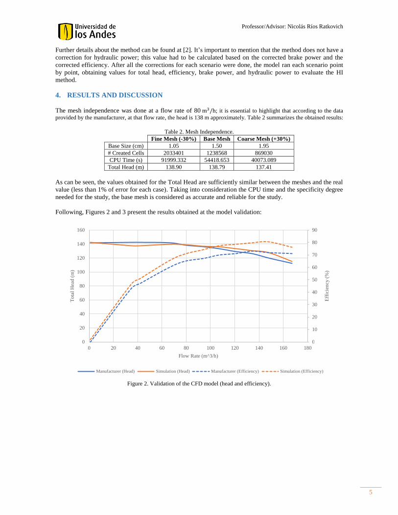
Following, Figures 2 and 3 present the results obtained at the model validation:

Figure 2. Validation of the CFD model (head and efficiency).

0%

10%

20%

30%

40%

50%

60%

70%

80%

90%

0

20

40

60

80

100

120

140

160

0 20 40 60 80 100 120 140 160 180

Eff

icie

ncy

(%

)

Tota

l H

ead

(m

)

Flow Rate (m^3/h)

Manufacturer (Head) Simulation (Head) Manufacturer (Efficiency) Simulation (Efficiency)


6

Figure 3. Validation of the CFD model (hydraulic power).

As can be seen, the simulation shows sufficiently accurate results based on the supplied data. Averaged

percentual error was 2.61% for the total head, 9.47% for efficiency, and 6.36% for hydraulic power. Table A3

in annexes show the data supplied by the manufacturer, simulation results, and percentual error per point. It’s

important to highlight that experimental conditions of the provided data are unknown, as well as the possible

errors that could be committed during that experimentation; efficiency and hydraulic power error are attributed

to that, even there are not that high. Instead of that, as the head is the most critical parameter to be evaluated in

this study, the model is considered as accurate and reliable for this purpose. According to the obtained results,

for the HI method evaluation, simulated total head uncertainty, efficiency uncertainty, and hydraulic power

uncertainty are defined at 3%, 10%, and 7%, respectively.

According to the HI method, parameter B must be between 1 and 40 to the procedure to be suitable. Table 3

shows the value obtained for the parameter per scenario:

Table 3. Parameter B per scenario.

Scenario B

1 1.5761

2 4.9841

3 15.7611

4 25.2467

The procedure is suitable for each scenario. Following, the results obtained for the HI method evaluation are

presented and summarized in the following figures:

0

10

20

30

40

50

60

70

80

0 20 40 60 80 100 120 140 160 180

Hyd

rau

lic

Pow

er (

kW

)

Flow Rate (m^3/h)

Manufacturer Simulation


7

Figure 4. Results - Total Head.

Figure 5. Results - Efficiency.

60

70

80

90

100

110

120

130

140

150

0 20 40 60 80 100 120 140 160 180

Tota

l H

ead

(m

)

Flow Rate (m^3/h)

Scenario 1 (HI) Scenario 2 (HI) Scenario 3 (HI) Scenario 4 (HI)

Scenario 1 (SIM) Scenario 2 (SIM) Scenario 3 (SIM) Scenario 4 (SIM)

0%

10%

20%

30%

40%

50%

60%

70%

80%

0 20 40 60 80 100 120 140 160 180

Eff

icie

ncy

(%

)

Flow Rate (m^3/h)




8

Figure 6. Results - Brake Power.

Figure 7. Results - Hydraulic Power.

As it is known, the total head is the measure of the height of a fluid column at the exit of the pump, and it

depends on the pressure rise given by the device, the properties of the fluid, the acceleration due to gravity,

among others. Figure 4 presents the comparison between the HI method and the simulation for the head. As can

be seen, the behavior of the head for the HI method and the simulation for each scenario matches with theory.

As the flow rate has lower values, fluid experiences lower friction losses as the flow are not so turbulent; the

head must be at its maximum value. On the other hand, as the flow rate increases, the flow becomes more

turbulent, which increases the possibility of the fluid to experience higher friction losses, leading the head to

decrease and eventually become zero.

0

20

40

60

80

100

120

140

0 20 40 60 80 100 120 140 160 180

Bra

ke

Pow

er (

kW

)

Flow Rate (m^3/h)



0

10

20

30

40

50

60

0 20 40 60 80 100 120 140 160 180

Hyd

rau

lic

Pow

er (

kW

)

Flow Rate (m^3/h)




9

Following, with a viscosity increase, it is expected a flow rate decrease because there’s an increase of the inertial

forces and a higher friction factor between the fluid and the pump walls, as it can be seen in Figure 4.

Additionally, as viscosity increases, the overall pressure increment decreases; at higher viscosity and lower

flow rate, the trend becomes more linear due to a flow regime transition inside the pump from turbulent flow to

laminar flow [3].

Shastri et at. [6] developed an analysis about losses of centrifugal pumps and concluded that impeller friction

losses, volute friction losses, and disk friction losses are considered to lessen the friction effect on a centrifugal

pump. Also, they found that the significant loss considered are incidence losses at the impeller, which happens

when the direction of the relative velocity of the fluid at inlet does not match with the inlet blade angle.

Therefore, fluid cannot enter the blade passage smoothly by gliding along the blade surface. More importantly,

it was found that the incidence loss of head increases when the flow rate decreases.

Now, on Figure 4 it can be seen that for all the scenarios at the low flow rate, the error between the HI method

and the simulation is more significant and, as flow rate increases, this error decreases and the values of the total

head tend to converge. This happens because the HI method does not consider incidence losses on their

correction methods, they only consider mechanical, volumetric and disk friction losses (simulation consider all

possible losses) and, as mentioned above, incidence loss of head increases when the flow rate decreases.

Besides, it can be seen that when viscosity increases, the error mentioned increases as well; this behavior is also

explained by the incidence losses because, with a viscosity increase, inertial forces increase, so the gliding along

the blade surface leads to significant losses.

Following, due to the increase of inertial forces that higher viscosities implies, brake power is expected to

increase; also, is expected that the maximum flow rate and the maximum hydraulic power decreases because

the pump is not capable of applying higher pressure. In fact, those changes in brake power and hydraulic power

explain the values obtained for the efficiency, because with waterless brake power has to be applied in order to

achieve almost the same hydraulic power, so the efficiency is higher, while the pump requires more with viscous

fluids (see Figures 5, 6 and 7).

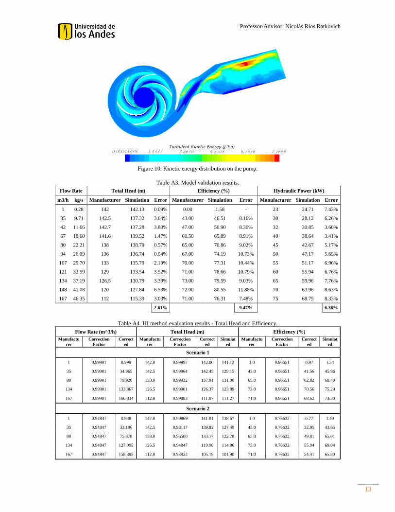
Centrifugal pumps are devices where fluid entering the pump receives kinetic energy from the impeller which

accelerates the liquid to a high velocity, transferring mechanical energy to the liquid to fulfill its duty. However,

volutes could have dead zones where the kinetic energy is high, and this energy cannot be transformed into

mechanical energy because the impeller does not rotate on that area, which represents work and pressure losses

on the pump. For this reason, manufacturers design pumps that minimize the probability of having dead zones

on the volute to increase efficiency.

As can be seen in Figure 7, the HI method makes a reliable estimation of the hydraulic power for all the

scenarios. However, on Figure 6 it can be seen that for the brake power the values obtained while the HI method

is overestimated, which influences directly over the efficiency results showed on Figure 5, which are

underestimated. As mentioned above, the HI method is based on test data available from sources throughout

the world and does not consider particular pump geometries, which means that it does not consider dead zones

that the simulation (geometry) do consider. For that reason, brake power is higher by the HI method, because

energy is being lost, needing more brake power to achieve the same hydraulic power, reducing efficiency. On

Figure 6 it’s also seen that, as the viscosity increases, the brake power error increases as well (increasing

efficiency error, consequently); what’s mentioned above explains it, because while the viscosity increases there

are major losses due to dead zones, needing even more brake power.

Finally, as discussed before, the experimental conditions of the supplied data are unknown, as well as the

possible errors that could be committed during that experimentation; consequently, the HI method calculations

have that error involved. On the other hand, the CFD model also involves an error, which can be associated

with the cell quality of the mesh (see Figures 8 and 9 in annexes), modelling and numerical error, etc. Modelling

errors, originating from the mathematical representation of the physical problem, are usually negligible in CFD

compared with numerical errors, which are due to the numerical solution of mathematical equations [3]. As

mentioned before, uncertainty on the obtained results (see Tables A4 and A5) has to be considered according

to the values presented previously.


10

5. CONCLUSIONS

The evaluation of the HI method for viscous corrections in centrifugal pumps trough CFD is presented in this

paper. Firstly, it is considered that the centrifugal pump performance parameters behave according to the theory

by the HI method and the CFD model. Following, the HI method does not consider incidence losses on their

correction methods, which are higher at the low flow rate, leading the HI method to overestimate the head at

off-design conditions. Additionally, when viscosity increases, inertial forces increases, so the gliding along the

blade surface leads to significant incidence losses. On the other hand, the HI method does not consider particular

pump geometries, which means that dead zones are not considered, simulation (geometry) do consider them.

Hence, brake power is higher by the HI method, because energy is being lost, needing more brake power to

achieve the same hydraulic power, reducing efficiency; while viscosity increases there are major losses due to

dead zones, requiring even more brake power. Finally, uncertainty on the calculations must be considered.

6. REFERENCES

[1] Reyes, L. H., Ríos, N., 2018. “Propiedades de los fluidos”. Operaciones Unitarias, Universidad de los

Andes.

[2] Hydraulic Institute, 2010. “Effects of Liquid Viscosity on Rotodynamic (Centrifugal and Vertical) Pump

Performance”.

[3] Zhu, J., et al., 2016. “CFD simulation and experimental study of oil viscosity effect on multi-stage electrical

submersible pump (ESP) performance.” J. Petrol. Sci. Eng.

[4] Nivea Pinto, R., Afzal, A., D’Souza, L. V., Ansari, Z., Mohammed, A. D., 2016. “Computational Fluid

Dynamics in Turbomachinery: A Review of State of the Art”. Archive of Computational Methods in

Engineering 24, pp. 467-479.

[5] Shah, S. R., Jain, S. V., Patel, R. N., Lakhera, V. J., 2013. “CDF for centrifugal pumps: a review of state

of the art”. Procedia Engineering 51, pp. 715-720.

[6] Shastri, R., Kumar, A., Kumar, M., 2014. “Analysis about losses of centrifugal pump by Matlab”.

International Journal of Computational Engineering Research 4, I9.

[7] 2018 Siemens Product Lifecycle Management Software Inc., 2018. “Simcenter STAR-CCM+

Documentation Version 13.04”. Simcenter STAR-CCM+ User Guide, 2018 Siemens PLM Software.

[8] Salim, M., Cheah, S., 2009. “Wall y+Strategy for Dealing with Wall-bounded turbulent flows” IMECS

[9] Ghyoot, C., 2012. “The modelling of particle build-up in shell-and-tube heat”. Potchefstroom Campus of

the North-West University 11.


11

ANNEXES

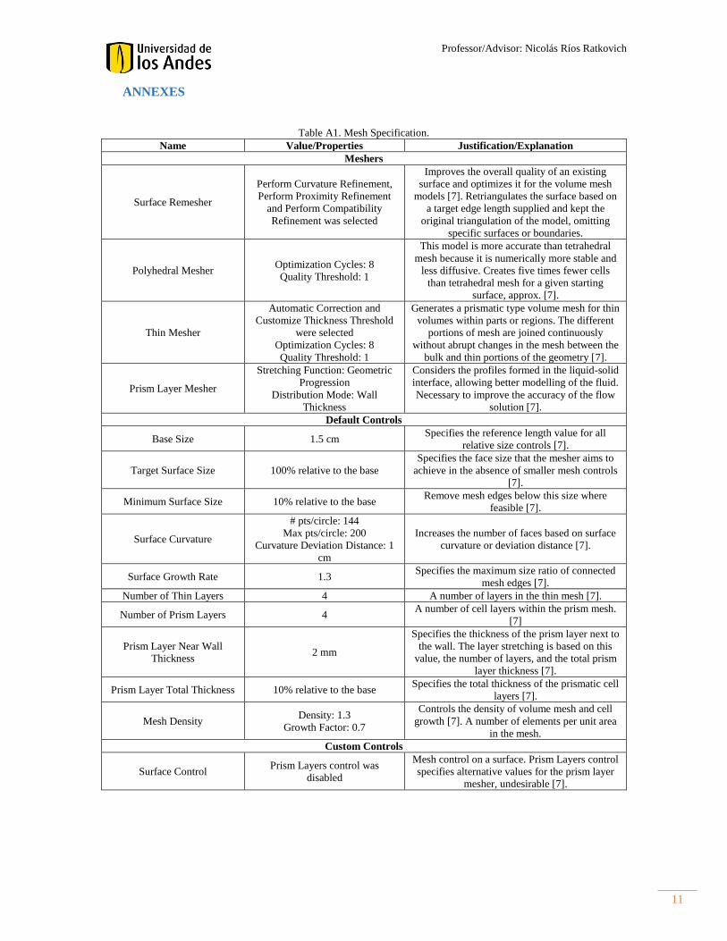
Table A1. Mesh Specification.

Name Value/Properties Justification/Explanation

Meshers

Surface Remesher

Perform Curvature Refinement,

Perform Proximity Refinement

and Perform Compatibility

Refinement was selected

Improves the overall quality of an existing

surface and optimizes it for the volume mesh

models [7]. Retriangulates the surface based on

a target edge length supplied and kept the

original triangulation of the model, omitting

specific surfaces or boundaries.

Polyhedral Mesher Optimization Cycles: 8

Quality Threshold: 1

This model is more accurate than tetrahedral

mesh because it is numerically more stable and

less diffusive. Creates five times fewer cells

than tetrahedral mesh for a given starting

surface, approx. [7].

Thin Mesher

Automatic Correction and

Customize Thickness Threshold

were selected

Optimization Cycles: 8

Quality Threshold: 1

Generates a prismatic type volume mesh for thin

volumes within parts or regions. The different

portions of mesh are joined continuously

without abrupt changes in the mesh between the

bulk and thin portions of the geometry [7].

Prism Layer Mesher

Stretching Function: Geometric

Progression

Distribution Mode: Wall

Thickness

Considers the profiles formed in the liquid-solid

interface, allowing better modelling of the fluid.

Necessary to improve the accuracy of the flow

solution [7].

Default Controls

Base Size 1.5 cm Specifies the reference length value for all

relative size controls [7].

Target Surface Size 100% relative to the base

Specifies the face size that the mesher aims to

achieve in the absence of smaller mesh controls

[7].

Minimum Surface Size 10% relative to the base Remove mesh edges below this size where

feasible [7].

Surface Curvature

# pts/circle: 144

Max pts/circle: 200

Curvature Deviation Distance: 1

cm

Increases the number of faces based on surface

curvature or deviation distance [7].

Surface Growth Rate 1.3 Specifies the maximum size ratio of connected

mesh edges [7].

Number of Thin Layers 4 A number of layers in the thin mesh [7].

Number of Prism Layers 4 A number of cell layers within the prism mesh.

[7]

Prism Layer Near Wall

Thickness 2 mm

Specifies the thickness of the prism layer next to

the wall. The layer stretching is based on this

value, the number of layers, and the total prism

layer thickness [7].

Prism Layer Total Thickness 10% relative to the base Specifies the total thickness of the prismatic cell

layers [7].

Mesh Density Density: 1.3

Growth Factor: 0.7

Controls the density of volume mesh and cell

growth [7]. A number of elements per unit area

in the mesh.

Custom Controls

Surface Control Prism Layers control was

disabled

Mesh control on a surface. Prism Layers control

specifies alternative values for the prism layer

mesher, undesirable [7].


12

Table A2. Physics Specification.

Models

All y+ Wall Treatment

The y+ is a non-dimensional distance used to

illustrate how coarse or fine a mesh is for a

particular flow. This model was chosen since it

incorporates methods for both coarse and fine

meshes [8].

Constant Density

The fluid is considered as incompressible,

which implies that the operating pressure has no

bearing on the calculation [7].

Exact Wall Distance

Makes an exact projection calculation in real

space for the wall distance, based on a

triangulation on a surface mesh [7].

Gradients Used within the transport equation solution

methodology [7].

K-Omega Turbulence It is used to model the turbulence using RANS

equations [7].

Liquid Fluids are liquid.

Reynold-Averaged Navier-Stokes Partial equations that describe the kinetic energy

and the rate of dissipation [7].

Segregated Flow

Solves the velocity and pressure equations,

linking the momentum transport and continuity

equations utilizing the SIMPLE algorithm [9].

SST (Menter) K-Omega

This model adds to the Standard K-Omega

model, an additional non-conservative cross-

diffusion term [7].

Steady Steady-state.

Three Dimensional Allows seeing the behavior of the fluids.

Turbulent Considering the Reynolds number, the turbulent

viscous regime is selected by default.

Reference Values

Minimum Allowable Wall

Distance: 1 ∗ 10−6 m

The minimum wall distance allowed within the

continuum [7].

Reference Pressure: 101325 Pa The absolute pressure value relative to which all

other pressures are defined [7].

Initial Conditions Pressure: 74980.5 Pa Working pressure profile [7].

Velocity: [0,0,0] m/s Velocity profile [7].

Figure 8. Mesh Cell Quality - Transversal view.

Figure 9. Mesh Cell Quality - Impeller.


13

Figure 10. Kinetic energy distribution on the pump.

Table A3. Model validation results.

Flow Rate Total Head (m) Efficiency (%) Hydraulic Power (kW)

m3/h kg/s Manufacturer Simulation Error Manufacturer Simulation Error Manufacturer Simulation Error

1 0.28 142 142.13 0.09% 0.00 1.58 - 23 24.71 7.43%

35 9.71 142.5 137.32 3.64% 43.00 46.51 8.16% 30 28.12 6.26%

42 11.66 142.7 137.28 3.80% 47.00 50.90 8.30% 32 30.85 3.60%

67 18.60 141.6 139.52 1.47% 60.50 65.89 8.91% 40 38.64 3.41%

80 22.21 138 138.79 0.57% 65.00 70.86 9.02% 45 42.67 5.17%

94 26.09 136 136.74 0.54% 67.00 74.19 10.73% 50 47.17 5.65%

107 29.70 133 135.79 2.10% 70.00 77.31 10.44% 55 51.17 6.96%

121 33.59 129 133.54 3.52% 71.00 78.66 10.79% 60 55.94 6.76%

134 37.19 126.5 130.79 3.39% 73.00 79.59 9.03% 65 59.96 7.76%

148 41.08 120 127.84 6.53% 72.00 80.55 11.88% 70 63.96 8.63%

167 46.35 112 115.39 3.03% 71.00 76.31 7.48% 75 68.75 8.33%

2.61% 9.47% 6.36%

Table A4. HI method evaluation results - Total Head and Efficiency.

Flow Rate (m^3/h) Total Head (m) Efficiency (%)

Manufactu

rer

Correction

Factor

Correct

ed

Manufactu

rer

Correction

Factor

Correct

ed

Simulat

ed

Manufactu

rer

Correction

Factor

Correct

ed

Simulat

ed

Scenario 1

1 0.99901 0.999 142.0 0.99997 142.00 141.12 1.0 0.96651 0.97 1.54

35 0.99901 34.965 142.5 0.99964 142.45 129.15 43.0 0.96651 41.56 45.96

80 0.99901 79.920 138.0 0.99932 137.91 131.00 65.0 0.96651 62.82 68.40

134 0.99901 133.867 126.5 0.99901 126.37 123.89 73.0 0.96651 70.56 75.29

167 0.99901 166.834 112.0 0.99883 111.87 111.27 71.0 0.96651 68.62 73.30

Scenario 2

1 0.94847 0.948 142.0 0.99869 141.81 138.67 1.0 0.76632 0.77 1.40

35 0.94847 33.196 142.5 0.98117 139.82 127.49 43.0 0.76632 32.95 43.65

80 0.94847 75.878 138.0 0.96500 133.17 122.78 65.0 0.76632 49.81 65.01

134 0.94847 127.095 126.5 0.94847 119.98 114.86 73.0 0.76632 55.94 69.04

167 0.94847 158.395 112.0 0.93922 105.19 101.90 71.0 0.76632 54.41 65.80


14

Scenario 3

1 0.74805 0.748 142.0 0.99360 141.09 121.02 1.0 0.36378 0.36 0.97

35 0.74805 26.182 142.5 0.90795 129.38 112.84 43.0 0.36378 15.64 31.44

80 0.74805 59.844 138.0 0.82888 114.39 103.15 65.0 0.36378 23.65 48.97

134 0.74805 100.239 126.5 0.74805 94.63 89.04 73.0 0.36378 26.56 47.61

167 0.74805 124.925 112.0 0.70282 78.72 77.13 71.0 0.36378 25.83 43.77

Scenario 4

1 0.62058 0.621 142.0 0.99037 140.63 118.52 1.0 0.19421 0.19 0.81

35 0.62058 21.720 142.5 0.86137 122.75 107.36 43.0 0.19421 8.35 28.20

80 0.62058 49.646 138.0 0.74230 102.44 94.79 65.0 0.19421 12.62 37.40

134 0.62058 83.158 126.5 0.62058 78.50 75.82 73.0 0.19421 14.18 34.88

167 0.62058 103.637 112.0 0.55246 61.88 61.84 71.0 0.19421 13.79 30.31

Table A5. HI method evaluation results - Brake Power and Hydraulic Power.

Flow Rate (m^3/h) Brake Power (kW) Hydraulic Power (kW)

Manufacturer Correction Factor Corrected Manufacturer Corrected Simulated Corrected Simulated

Scenario 1

1 0.99901 0.999 23 39.64 24.86 0.38 0.38

35 0.99901 34.965 30 32.37 26.76 13.45 12.30

80 0.99901 79.920 45 47.39 41.68 29.77 28.51

134 0.99901 133.867 65 64.76 59.98 45.69 45.16

167 0.99901 166.834 75 73.46 68.96 50.41 50.54

Scenario 2

1 0.94847 0.948 23 47.41 25.60 0.36 0.36

35 0.94847 33.196 30 38.05 26.40 12.54 11.52

80 0.94847 75.878 45 54.79 39.02 27.29 25.37

134 0.94847 127.095 65 73.63 57.57 41.19 39.75

167 0.94847 158.395 75 82.71 66.80 45.00 43.95

Scenario 3

1 0.74805 0.748 23 78.37 25.46 0.29 0.25

35 0.74805 26.182 30 58.49 25.59 9.15 8.04

80 0.74805 59.844 45 78.19 34.32 18.49 16.81

134 0.74805 100.239 65 96.48 51.04 25.62 24.30

167 0.74805 124.925 75 102.84 59.94 26.56 26.24

Scenario 4

1 0.62058 0.621 23 121.38 24.76 0.24 0.20

35 0.62058 21.720 30 86.23 22.52 7.20 6.35

80 0.62058 49.646 45 108.82 34.26 13.74 12.81

134 0.62058 83.158 65 124.37 49.22 17.63 17.17

167 0.62058 103.637 75 125.61 57.58 17.32 17.45


15

Figure 11. Manufacturer performance curves.

Figure 12. Clyde Union Pumps Ref. RP1A26.

Evaluation of the Hydraulic Institute method for viscous ...

Documents

Transcript of Evaluation of the Hydraulic Institute method for viscous ...