Loughborough UniversityInstitutional Repository

Evaluation of the controlsaffecting the quality of

spatial data derived fromhistorical aerial photographs

This item was submitted to Loughborough University's Institutional Repositoryby the/an author.

Citation: WALSTRA, J., CHANDLER, J.H., DIXON, N. ...et al., 2011. Eval-uation of the controls affecting the quality of spatial data derived from histor-ical aerial photographs. Earth Surface Processes and Landforms, 36 (7), pp.853�863.

Additional Information:

• This article was published in the journal, Earth Surface Processes andLandforms [ c© John Wiley & Sons, Ltd.] and the definitive version isavailable at: http://dx.doi.org/10.1002/esp.2111

Metadata Record: https://dspace.lboro.ac.uk/2134/8998

Version: Accepted for publication

Publisher: c© John Wiley & Sons, Ltd.

Please cite the published version.

This item was submitted to Loughborough’s Institutional Repository (https://dspace.lboro.ac.uk/) by the author and is made available under the

following Creative Commons Licence conditions.

For the full text of this licence, please go to: http://creativecommons.org/licenses/by-nc-nd/2.5/

Evaluation of the controls affecting the quality of spatial data derived from historical aerial photographs

Jan Walstra1, Jim H. Chandler

2, Neil Dixon

2 & Rene Wackrow

2

1 Department of Languages & Cultures of the Near East & North Africa, Ghent University, Ghent, Belgium

2 Department of Civil and Building Engineering, Loughborough University, Loughborough, UK

Abstract

This paper is concerned with the fundamental controls affecting the quality of data derived

from historical aerial photographs typically used in geomorphological studies. A short review

is provided of error sources introduced into the photogrammetric workflow. Datasets from

two case-studies provided a variety of source data and hence a good opportunity to evaluate

the influence of the quality of archival material on the accuracy of coordinated points. Based

on the statistical weights assigned to the measurements, precision of the data was estimated a

priori, while residuals of independent checkpoints provided an a posteriori measure of data

accuracy. Systematic discrepancies between the two values indicated that the routinely used

stochastic model was incorrect and overoptimistic. Optimised weighting factors appeared

significantly larger than previously used (and accepted) values. A test of repeat measurements

explained the large uncertainties associated with the use of natural objects for ground control.

This showed that the random errors not only appeared to be much larger than values accepted

for appropriately controlled and targeted photogrammetric networks, but also small

undetected gross errors were induced through the ‘misidentification’ of points. It is suggested

that the effects of such ‘misidentifications’ should be reflected in the stochastic model through

selection of more realistic weighting factors of both image and ground measurements. Using

the optimised weighting factors, the accuracy of derived data can now be more truly

estimated, allowing the suitability of the imagery to be judged before purchase and

processing.

Keywords: digital photogrammetry, historical aerial photograph, data quality, error

assessment

Introduction

Photogrammetry is an effective tool in geomorphological studies (Lane et al., 1993; Chandler,

1999). Aerial photographs not only give a qualitative description of the Earth’s surface, but

also provide a metric model from which quantitative measurements can be obtained. The

photographic film archive is increasingly accessible to the public (e.g. USGS, 1997; NAPLIB,

1999) and a suitable sequence over time representing a site allows morphological changes to

be determined if appropriate photogrammetric methods are used. The automation afforded by

modern digital photogrammetric techniques have allowed for rapid and cost-effective data

collection (Chandler, 1999; Baily et al., 2003).

An important aspect of any quantitative analysis is assessing the quality of data. As pointed

out by some authors (Fryer et al., 1994; Cooper, 1998; Lane et al., 2000), the ease of which

terrain data may be generated using highly automated techniques has focussed attention more

on the analysis and interpretation of results and less on the issues of data quality. Digital

Elevation Models (DEMs) are by far the most commonly used photogrammetric product

among geomorphologists and an important aspect of their creation is stereo-matching based

on automated algorithms. Many users typically consider these automated procedures as being

the single most important factor affecting DEM quality, thereby overlooking the importance

of the underlying photogrammetric model. Lane et al. (2000) thoroughly explored the effects

of automated stereo-matching on overall surface representation, but concluded these were

only little, and it is rather the design of the photogrammetric survey that is of primary

importance. Hence, whether data processing is manual or automated, the fundamental controls

of image geometry and image coordinate precision are of primary importance for data quality.

These are known as first and second order photogrammetric network design (Fraser, 1984;

Cooper, 1987; Fraser, 2007).

What is perhaps more surprising is the lack of research that has focussed on these

conventional controls in a consistent way. In geomorphological studies, often material is used

that is readily available, but not intended for such use. Some claims made for accuracy are

based on conventional air surveys collected for mapping purposes, while others are based on

very case-specific studies. Moreover, examples in literature rarely use propagation of variance

to estimate precision of derived parameters as a function of the precision of the original

source data (Fryer et al., 1994). This is a crucial practice, especially when dealing with

archival material with little control over source data quality, and the required accuracy should

be considered beforehand.

The aim of this study is to evaluate the fundamental controls on photogrammetric data quality

in the context of archival (film) imagery. The outcomes should allow the formulation of a

priori measures of data accuracy based on the characteristics of available material. Such

information would be of great value to users of historical imagery, as it allows their suitability

for the intended purpose to be judged prior to purchase and processing. Two case-studies

(Walstra et al., 2007) provided the necessary variety of source data for these explorations.

Although digital airborne cameras have been around for a decade now, film cameras are still

widely employed (Cramer, 2005; Petrie and Walker, 2007) and, of course, remain the primary

origin of archival material. This study is therefore concerned only with (scanned) material

from film archives.

Photogrammetric principles: functional and stochastic model

Restitution is the procedure of establishing appropriate functional and stochastic models for

describing the relationship between ground and photo coordinates. In many modern software

systems, analytical photogrammetry methods established 30-100 years ago provide the basis

for the restitution.

The functional model

Analytical photogrammetry entails the formulation of a rigorous mathematical relationship

between measured ground and photo coordinates, and camera parameters. The main principle

is the concept of collinearity, in which an object, the projection centre and its corresponding

point appearing on the focal plane of the camera, all lie along a straight line. Based on this

principle, and provided that the interior and exterior orientation of the camera are known, 3D

coordinates can be extracted from a stereo-pair of photographs.

For aerial film cameras, calibration certificates include the parameters of interior orientation:

the location of the principal point, focal length, photo coordinates of the fiducial marks, and

measures of lens distortion (Wolf and Dewitt, 2000). The exterior orientation parameters,

representing the position and orientation of each photograph (typically unknown before the

advent of GPS and inertial navigation systems), need to be resolved in a so-called "bundle

adjustment". This is an iterative procedure in which the positions of the frames are

simultaneously determined in a single least squares solution and involving linearized

collinearity equations. Tie points connect adjacent photographs, while control points fix the

solution into an object coordinate system. The unknowns associated with a bundle adjustment

are the object coordinates of the tie points and the exterior orientation parameters of all

photographs. The measured elements include the photo coordinates of tie and control points,

and ground coordinates of control points, all weighted according to their presumed precision.

Advantages of the procedure include: mathematical rigour, reduced ground control

requirements and the minimisation and distribution of errors among all image frames.

For accurate photogrammetric work, corrections need to be made for various effects, which

otherwise may result in systematic errors. These include: lens and film distortions,

atmospheric refraction, earth curvature and deformation of the photos during the developing

process and storage (Jacobsen, 1998; Wolf and Dewitt, 2000). The scanning process, which is

an unavoidable practice when converting historical (film) imagery into digital form, may

introduce further distortions.

The bundle adjustment offers the flexibility of incorporating additional parameters for

estimating unknown camera parameters (if there is no calibration certificate available) and

any systematic distortions. In that case, the procedure is known as a “self-calibrating bundle

adjustment” (Brown, 1956; Kenefick et al., 1972; Granshaw, 1980; Chandler and Cooper,

1989). However, the inclusion of extra unknowns requires more measurements and significant

correlation between parameters may lead to unsatisfactory results.

Once the mathematical relationship between the photographs and the ground surface has been

established, coordinates can be extracted from anywhere on the site, and used to create DEMs

and orthophotos. Since the 1990s, significant developments in digital photogrammetry have

allowed automation of large parts of the photogrammetric workflow (e.g. Schenk, 1996), but

detailed description of these are beyond the scope of this paper.

The stochastic model

Measurements can be regarded as random variables. By eradicating gross errors and

minimising the effects of systematic errors it can be assumed that only random errors remain.

These can be described by the variances of the measurements, the so-called stochastic model.

The inclusion of a stochastic model in a bundle adjustment allows measurements of differing

quality to be combined in a rigorous way. All measurements are weighted according to their

prescribed variances, which are subsequently propagated through the functional model,

thereby providing estimates of the variances of derived data (Cooper and Cross, 1988; Butler

et al., 1998).

All of these functional and stochastic aspects are of great importance when historical

photographs are used. The perfect historical data set is rarely available and the lack of

redundant imagery requires judgement to assess whether an appropriate stochastic and

functional model has been achieved.

Data quality: controls and evaluation

As defined by Cooper and Cross (1988), the quality of derived data is a function of the

precision, accuracy and reliability of the measurements and the functional model used.

Precision can be related to random errors inherent in any measurement procedure, accuracy

can be associated with systematic errors in the model, while reliability refers to the presence

of gross errors.

Precision

The precision of image measurements is inherent to the source data, and a function of the

resolving power or sharpness of the lens and film used. The resolving power of a photograph

can be described by its spatial frequency (lines/mm) and the contrast. The resolving power of

a typical photogrammetric camera is usually limited by the film rather than by the lens or

image motion during exposure (Slama, 1980). Other factors are the atmospheric conditions,

target contrast, and film processing. The grain size of the silver crystals in film emulsions

provides a much better resolving power than can be achieved using paper prints. In general,

colour films are grainier than black-and-white film, and grains tend to be larger in older

material due to lower quality of the emulsions (Lo, 1976).

Although the pixel resolution is an important control for both scanned, and indeed directly

acquired digital, imagery, the quality of the lens remains paramount (Thomson, 2010). In

order to preserve an original film resolution of 30-60 lines/mm, a scanned pixel size of 6-12

µm would be needed. For many practical applications, such as DEM generation, good results

can be achieved with 25-30 µm resolution (Baltsavias, 1999).

The effects of photo-scale and image resolution can be combined conveniently in terms of

ground resolution, which determines the level of horizontal detail in object space that is

visible on the photographs (Lillesand and Kiefer, 1994). Using trigonometry, an approximate

estimate for the corresponding vertical resolution can be obtained by multiplying the

horizontal ground resolution with the inverse base/height ratio (Equations 1 and 2). It follows

that a strong convergence (large base/height ratio), and consequently large relief

displacement, gives rise to precise vertical object coordinates (Wolf and Dewitt, 2000).

(Equation 1) Ssr

SHR x ⋅==

(Equation 2)B

HSs

B

H

r

SVR x ⋅⋅=⋅=

Where HR and VR are horizontal and vertical ground resolution respectively, S is scale number, r is image

resolution, sx is pixel size, H is flying height and B is base distance between the stereo-images.

The precision of ground control measurements depends on the surveying technique used. For

photoscales of 1/4,000-1/50,000 the use of differential GPS (dGPS) is recommended

(Chandler, 1999). The precision of dGPS (stop and go, post processed) is typically in the

order of 10-20 mm +1 ppm horizontally and 20-30 mm +1 ppm vertically (Uren and Price,

2006). When less precise ground data is used, such as topographical maps, these may

introduce significant errors in the bundle adjustment.

Accuracy

Accuracy can be related to the presence of uncorrected systematic errors and other

deficiencies in the functional model. Accounting for all unknown systematic effects in a self-

calibrating bundle adjustment is difficult because many cannot be modelled explicitly, and

there is usually high correlation between the modelling parameters. Consequently, the

mathematical model remains an approximation and provides a limiting constraint on the

quality of derived data. Systematic errors may also arise from inaccurate or poorly distributed

control points (Mills et al., 2003), which should be evenly distributed over the images to

develop strong geometry, and ideally surround the volume of interest (Chandler, 1999). In

theory only three points are required to define a datum, but in practice more control points are

desirable as redundancy provides appropriate checks and allows a precision of the solution to

be determined (Wolf and Dewitt, 2000).

The only way to quantify the accuracy of a photogrammetric solution is to compare calculated

coordinates with accepted values. Traditionally, accuracy is evaluated by computing the

global root-mean-square error (RMSE) of independent checkpoints. The combination of mean

and standard deviation of error (ME and SDE) is more appropriate in a statistical sense (Li,

1988) and can be used to distinguish between the unwanted systematic errors (ME) and the

expected and tolerable random effects (SDE) (Lane et al., 2003; Chandler et al., 2005).

Reliability

Reliability can be related to gross errors, and the ease with which they may be detected

(Cooper and Cross, 1988). Gross errors are genuine mistakes or blunders that arise during

photogrammetric measurement, for example misidentified or mistyped control points or

mismatching in the process of automatic tie-point generation. Fortunately, gross errors are

normally easy to detect and eradicate because of their size. Residuals of the control points in a

bundle adjustment reflect the difference between measured and estimated values – large

residuals indicate gross errors that can be interactively removed or corrected by the operator.

Small gross errors that remain undetected will have a negative effect upon the accuracy of the

derived data (Lane et al., 2003).

Data-sets from two case-studies

Photogrammetric techniques were applied in two case-studies, both concerning active

landslides in the UK: the Mam Tor landslide in Hope Valley, Derbyshire (Ordnance Survey

grid reference SK135835) and the East Pentwyn landslide in Ebbw Fach Valley, South Wales

Coalfield (SO207075). Both landslides showed considerable movements over the last 50

years, were subject to frequent investigations in the past and are covered by a range of

historical photography of varying quality. The working process adopted can be summarized in

four general stages:

1. Search and acquisition of suitable imagery from archives (Figure 1)

2. Collection of precise ground control

3. Photogrammetric restitution and data extraction

4. Visualization and analysis of the data

A range of data products was derived from the image sequences and explored for analysing

geomorphological change occurring on the landslides. These products included

geomorphological maps, ‘DEMs of difference’, displacement vectors (Figure 2) and

animations. An extensive description of the case-studies is provided by Walstra et al. (2007).

(Figure 1)

(Figure 2)

The datasets

The photographic sequence acquired for the Mam Tor case-study comprised seven epochs,

representing a variety of formats, scales, media and qualities (Figure 1 and Table 1). In

general, camera parameters were readily available from calibration certificates and the

photogrammetric restitution was straightforward. Only in the case of the MT-1953 and MT-

1971 epochs were calibration files lacking, and these had to be estimated in a self-calibrating

bundle adjustment.

For the East Pentwyn case-study four epochs were acquired (Table 2). Calibrated camera

parameters were available only for the EP-1971 images. Although the EP-1973 epoch was

captured with a metric camera, a calibration certificate was lacking. The fiducial marks

allowed an estimation of the principal point position, and values for the focal length and

flying height were derived from the data strip displayed on the side of the frames. Self-

calibration did not lead to any significant improvements to the camera model, and so these

rather crude parameter values had to be accepted. The RAF imagery (EP-1951 and EP-1955)

presented a challenge because they exhibited large systematic distortions that could not be

modelled; consequently an unsatisfactory camera model had to be adopted.

The achieved accuracies of the solutions are displayed in Table 3. It should be noted that the

quoted errors are based on a limited number of checkpoints. The absence of systematic errors

(except for EP-1955) is confirmed by insignificant ME values (relatively small compared to

the SDE values) and validates the photogrammetric solutions, including the self-calibrating

adjustments of MT-1953 and MT-1971. The large errors of the epochs EP-1951, EP-1955 and

EP-1973 result from the inadequate camera model used, while the poor accuracy of MT-1953

can be attributed to the use of poor-quality scanned contact prints. The vertical accuracy is

usually worse than horizontal, as is inherent to the geometry of standard aerial surveys (cf.

Equation 2).

(Table 1)

(Table 2)

(Table 3)

Software and equipment

High-precision geodetic GPS receivers and differential methods were used for collecting

ground control. For the Mam Tor case-study a combination of Leica system 200 and 300

single frequency receivers was used for the surveying. For the other case-study a set of Leica

system 500 dual frequency receivers was available. Control points were measured and post

processed in a ‘stop-and-go’ type of survey, resulting in an accuracy of approximately 0.01 m.

Post-processing of the GPS data was performed by using Leica’s SKI-Pro software, version

2.5.

All of the photogrammetric work described in this paper was processed on a moderately

equipped PC using Leica Photogrammetry Suite (LPS) software, version 9, except for the

self-calibration procedures, which were performed in the external General Adjustment

Program (GAP) developed by Chandler and Clarke (1992). Statistical analyses were carried

out using SPSS software, version 15.

Error analysis

As pointed out earlier, propagation of variance can be used to estimate the precision of

derived parameters as a function of the original source data. This practice is crucial also to

ensure an appropriate balance between the functional and stochastic models. The

appropriateness of the stochastic model can be analysed by comparing the a priori value of

the variance factor with the a posteriori value, which should be identical. Strictly comparison

should be based on an F Test (Cooper, 1987) , but in practice an a posteriori factor of 1-1.5

can be simply accepted at 0.05 levels of significance. A priori analysis allows a covariance

matrix of the estimated parameters to be obtained, based on the statistical weights assigned to

the measurements. This also allows an estimation of the precision of the estimated data. The a

posteriori variance factor is based on the actual residuals of the bundle adjustment, in relation

to the assigned weightings. A significant difference (i.e. >1.5) between the two variance

factors can be ascribed to a number of causes: errors in the computations, undetected

systematic errors or blunders, inaccurate linearization of the functional model and/or a wrong

stochastic model (Cooper, 1987).

The only global indicator for the quality of the adjustment provided by LPS is the ‘total RMS

error of solution’. This indicator does not relate to classical error theory described above, but

is useful for the layperson, since it is derived from all residuals of the adjustment and

expressed in image coordinate units, which is generally more meaningful to the user. In this

study it was attempted to analyse the variance of the output data in a more rigorous way,

principally in evaluating more fully the stochastic models used and identifying the main

variables controlling data accuracy. Despite this rigour, it is recognised that this approach is

based on rather limited datasets and is therefore inevitably speculative. Also, it was assumed

that any gross errors in the bundle adjustment were successfully removed, and that all

variance in the final data were solely due to random errors and perhaps small unresolved

systematic errors.

A common measure of accuracy is the (root-) mean-square-error (MSE), defined as the sum

of variances of random errors and bias (Equation 3) (Mikhail and Gracie, 1981).

(Equation 3) 22 βσ +=MSE

Where MSE is mean-square-error, σ2 is a measure of the variance of random errors and β

2 represents the variance

of bias (defined as the difference between mean value and true value).

A simplified way of estimating the expected accuracy in a bundle adjustment would be by

summing the contributed variances from both image and ground measurements, provided

these are in the same coordinate system and units (Equation 4).

(Equation 4) 222

io σσσ +=Σ

Where Σσ2 is a measure of the total variance in the bundle adjustment, σo

2 is the variance of errors in object

measurements, and σi2 is the variance of errors in image measurements.

Equations 3 and 4 can be combined, and assuming the functional model is correct and

systematic errors are absent (β2 = 0), it follows that the accuracy of the output data from the

adjustment in theory should be directly related to the variance of the input measurements

(Equation 5).

(Equation 5) 22

ioMSE σσ +=

Where MSE is mean-square-error, σo2 is the variance of errors in object measurements, and σi

2 is the variance of

errors in image measurements.

Random errors are introduced in the adjustment procedure as standard deviations (σi and σo

for image and ground measurements, respectively). In line with recommendations by LPS (i.e.

use of values less than 1 pixel), initially, standard deviations of ±0.2 pixel were assigned to

the image measurements (variable a in the following analysis). These values were converted

into object dimensions by multiplying them by the image ground resolution (Equations 6 and

7). Standard deviations of 0.01 m were assigned to the ground control measurements, based

on the values from the GPS post-processing and already in object dimensions (variable b in

the following analysis; Equation 8). This latter contribution should be significant compared to

the image ground resolution only in the case of very large-scale imagery (i.e. epoch MT-

1973).

(Equation 6) HRaYXi ⋅=),(σ

(Equation 7) VRaZi ⋅=)(σ

(Equation 8) bZYXo =),,(σ

Where σi(X,Y) and σi(Z) are the standard deviations of image measurements in object dimensions, σo(X,Y,Z) are

the standard deviations of ground measurements, a and b are the weightings/precisions assigned to image and

ground measurements, and HR and VR are the horizontal and vertical ground resolution of the stereo-pair

(derived from Equations 1 and 2).

Substituting the values from Equations 6-8 into Equation 5 provided estimates of expected

total variance, or MSE, of the bundle adjustment as a function of the input data (Equations 9-

11). Since a single value for horizontal accuracy would be more useful than separate values

for arbitrary X and Y directions (stereo-pairs from different epochs are not oriented to the

same direction), these were combined through vector summation of σ(X) and σ(Y) (Equation

10).

(Equation 9) ( ) 22),( bHRaYXMSE +⋅=

(Equation 10) 222 22),(2)( bHRaYXMSEHorMSE +⋅=⋅=

(Equation 11) ( ) 22)( bVRaVerMSE +⋅=

Where MSE(X,Y) is the variance in either X or Y direction, MSE(Hor) is the combined horizontal variance,

MSE(Ver) is het vertical variance, HR and VR are horizontal and vertical ground resolution (derived from

Equations 1 and 2), and a and b are the weightings assigned to image and ground measurements (initially set at

0.2 and 0.01).

The estimates of a priori expected accuracy (in terms of RMSE) of all epochs were compared

to their corresponding a posteriori observed accuracy (in terms of SDE of checkpoints, from

Table 3). With no exceptions, the observed errors were significantly larger than expected

(Table 4). This suggests either the presence of unresolved systematic errors, or a significant

underestimation of the random errors in the stochastic model. The first option can be

dismissed judging from the insignificant mean errors observed (except for epochs EP-1951,

EP-1955 and EP-1973, see Table 3), and anyway would be unlikely for the epochs with full

camera calibration data available.

(Table 4)

The data were graphically displayed in order to look for any obvious trends (Figure 3), with

epochs grouped according to their camera calibration status. Although the number of data

points is little, at least for the epochs with fully calibrated camera models there seems to be a

linear relation between expected and observed accuracy. However, its slope is much gentler

than the ideal 1:1 line, suggesting that the stochastic model adopted was overoptimistic. For

two epochs (MT-1953 and MT-1971) the camera model was successfully estimated through

self-calibration, but some systematic errors may be left unresolved, perhaps due to the use of

poor-quality prints, resulting in a steeper trend. The three other epochs, in which the camera

model could not be resolved through self-calibration (EP-1973, EP-1951 and EP-1955), were

left out in further analysis as they were considered outliers.

(Figure 3)

In order to find a better balance between expected and observed accuracy, it was explored

how these uncertainties could be best reflected in the stochastic model,. Since σo2 (=2b

2) is

constant for all epochs (same source for ground control), Equation 10 can be treated as a

linear function between squared ground resolution and MSE. Assuming absence of systematic

errors, MSE should equal the variance of the checkpoints (squared SDE values, derived from

Table 3). The term 2a2 corresponds to the slope of this linear relation and 2b

2 to the intercept.

For the group of fully-calibrated epochs these terms were determined through regression

(Figure 4) and provided optimum values for the weighting parameters a and b (respectively

0.82 and 0.20 instead of the initially used 0.2 and 0.01).

The data-points of the two self-calibrated, poorly scanned epochs are situated beyond this line

(Figure 4), even if much more so for epoch MT-1953 than for MT-1971. In an attempt to

account for the additional errors inherent to using low-quality scanned prints, a similar

regression was carried out for this ‘group’ of points. Since the same ground control was used,

the precision in the object measurements was assumed identical; hence the intercept should be

the same as for the fully calibrated cameras. In this case, regression revealed a value of 2.55

for weighting parameter a.

(Figure 4)

Testing image measurement precision

The discrepancy between the initially assigned weighting parameters and the optimised values

suggest an underestimation of the errors in the image and/or ground measurements. Especially

the sub-pixel precision of image measurements seems a little too optimistic. Such a precision

may be feasible using artificial targets in a controlled photogrammetric network, but is clearly

unrealistic for the natural objects used as ground control in this study.

The only way to obtain a reliable estimate of ‘true’ precision is to obtain repeat measurements

and analyse the standard deviations of errors (Mikhail and Gracie, 1981). For this purpose, a

small subset of five control points was repeatedly measured on two individual photographs

from different epochs (MT-1953 and MT-1973). The points represent natural features

typically used for ground control and were actually used in the Mam Tor case-study. In this

experiment, each of the points was measured ten times on both images, in order to derive a

statistically valid dataset (i.e. with a precision of less than one standard deviation at the 0.01

level of significance). This procedure was completed by six different operators, including

three photogrammetric experts and three ‘non-experts’.

(Table 5)

(Table 6)

(Figure 5)

From the statistics (Tables 5 and 6) a number of conclusions can be drawn. First of all, the

standard errors of almost all measured points were considerably larger than 0.2 of a pixel.

There was a certain variation in standard errors between points, as well as between images

and between operators. The standard deviations of measurements ‘within’ operators (last

column) were computed by averaging the variances of all points for each operator. They

reflect the ability to repeatedly identify the same image point and strongly depend on the

distinctiveness and contrast of objects in the image, as well as on the operator’s skills

(although no clear distinction could be made between the performance of experts and ‘non-

experts’). These errors correspond to the random errors inherent to any measurement

procedure. Standard errors ‘within’ each operator ranged from 0.28-1.05 pixel for the MT-

1953 image and 0.64-4.53 for the MT-1973 image. On the other hand, the standard deviations

of measurements ‘between’ operators (lower rows), derived from combining measurements

from all operators for each point, appeared to be significantly larger – ranging from 0.40-3.60

pixel for the MT-1953 image and 0.90-15.43 for the MT-1973 image. Such large errors

clearly indicated discrepancies between operators in correlating ground features to their

‘correct’ image point, reflected in an offset between the estimated (mean) locations (and

hence potentially from their ‘true’ location). A clear example of such ‘misidentification’ is

illustrated by the measurements of point 2 in image MT-1973, with two point clouds

distinctively separate from the rest (Figure 5: operators A1 and B3). Normally such incorrect

measurements would be easily detected as gross errors and removed from the adjustment. In

other cases, such ‘misidentifications’ may be very subtle and hardly separable from random

measurement errors, thereby reducing the effective accuracy of the solution. An example of

such subtle ‘misidentification’ is illustrated by the measurements of point 2 in image MT-

1953, showing slightly off-set but still largely overlapping point clouds (Figure 5). On the

other hand, point 4 in image MT-1953 represents an excellent control point with perfectly

overlapping point clouds and standard errors ‘within’ and ‘between’ operators of comparable

size.

Discussion

Effects of ‘misidentification’ errors

The image measurement experiment demonstrated that standard errors are considerably larger

when dealing with natural objects, than the values routinely used in the stochastic models.

Indeed, this confirms the use of larger weightings for image measurements in bundle

adjustments as suggested by the error analysis in this study.

But, interestingly, the measurements from the poor quality image MT-1953 showed more

consistency than the better quality image MT-1973 (Table 5: overall SDE of 1.65 and 1.84 in

x/y versus 5.34 and 8.45). At first sight, this seems contrary to the accuracies observed in the

photogrammetric solutions of the two epochs (Table 3) and the subsequent argumentation in

this study which culminated in the assignment of larger weightings to the measurements from

poor quality imagery. A possible explanation would be that the effect of ‘misidentification’ of

image points is linked to image scale rather than directly proportional to pixel size. The exact

identification of a large object (e.g. the corner of a wall) may cause more trouble in the case

of larger-scale imagery, where the object extends over multiple pixels and thereby increasing

the chance and size (in pixel units) of ‘misidentification’. As such, it can be argued that the

effect of ‘misidentification’ should be reflected in the weightings of ground rather than image

measurements, so that their effect becomes relatively greater for larger-scale imagery. It also

explains the initially poor ratio between observed and expected accuracy of the MT-1973

epoch (Table 4).

Random errors are inherent to the (radiometric) quality of the available imagery, but the effect

of ‘misidentifications’ can only be reduced by selecting appropriate objects for ground

control. Suitable control points should be well-defined and undisputable features, both in the

field and on the imagery. Of course, if historical imagery is used, problems of accessibility

and site changes may limit the choice. And even if features seem appropriate for one pair of

images, this may be different for another (Figure 5: compare point 4 in MT-1953 and MT-

1971).

Controls on data quality

Apart from improvements to the stochastic model, Equations 10 and 11 also provide a means

to estimate the accuracy of coordinated points a priori, based on scanning resolution and

image scale. Furthermore, the analysis showed that the accuracy that can be achieved from

scanned prints may be up to a factor 3.1 (2.55/0.82) worse than scanned diapositives. Of

course this value is of limited significance, since it is based on very limited data, but it gives

an indication of the degenerating effect on accuracy, when poor-quality source material is

used.

Other factors that may affect data accuracy include the amount and distribution of control

points, and the quality of camera calibration data. Although the datasets in this study were too

limited to quantify all of these factors, an attempt to relate their effects is presented in Figure

6 (the scale bar provided is only a rough estimate). The top of this diagram represents the best

data quality that can be achieved using high-quality scanned contact-diapositives, a calibrated

metric camera model and high quality control data. The quality of source data degrades down

to the bottom of the diagram, with the worst results to expect from paper prints scanned with a

cheap desktop device (a factor of 3.1 compared to top quality). Regarding camera calibration,

still reasonable results can be achieved when the camera geometry is estimated in a self-

calibrating procedure, although this would strongly depend on the availability of high quality

ground control. Ground control will be a limiting factor when its accuracy is low compared to

the image ground resolution or when its spatial distribution within the images is poor.

A more global factor for long-term stability of the photographic record could also be

considered in such analysis. Such a term would incorporate different effects such as camera

and film quality, and reliability of ground control (i.e. did control points really remain

unchanged). These factors all deteriorate with increasing age but their effects are difficult to

separate and quantify.

Figure 6.

Conclusion

The aim of this study was to evaluate the controls on photogrammetric data quality in the

context of archival (film) imagery, typically used in geomorphological studies. Systematic

analysis showed that uncertainties associated with image measurements of natural objects are

larger than the values routinely used and accepted for appropriately controlled and targeted

photogrammetric networks. Limited distinctiveness and contrast of the objects aversely affect

the size of random errors, while small ‘misidentifications’ may lead to undetected gross

errors. It is suggested that the effects of such ‘misidentifications’ should be reflected in the

standard deviations assigned to ground rather than image measurements in the adjustment.

Based on a variety of source data used in two case-studies, optimised weighting factors for the

stochastic model were estimated, which appeared significantly larger than previously used

values: a standard error of 0.82 of a pixel for image measurements and 0.20 m for dGPS

ground control measurements. The analysis also showed that the data accuracy from scanned

prints may be up to 3.1 times worse than from photogrammetric-quality scanned diapositives.

Using these insights, accuracy of derived data can now be estimated a priori and its suitability

judged, based on the characteristics of the imagery.

Acknowledgements

Most of the work described in this paper was carried out at the Department of Civil and

Building Engineering, Loughborough University, and formed part of the lead author’s

doctoral thesis (available online: Walstra, 2006). ‘Non-expert’ colleagues from Ghent (Meins

Coetsier, Guido Suurmeijer and Peter Verkinderen) are thanked for participating in the image

measurements. Two anonymous reviewers are thanked for valuable comments on an earlier

draft of this paper.

Bibliography

Baily, B., Collier, P., Farres, P. J., Inkpen, R., Pearson, A., 2003. Comparative assessment of

analytical and digital photogrammetric methods in the construction of DEMs of

geomorphological forms. Earth Surface Processes and Landforms, 28 (3), pp. 307-320.

Baltsavias, E. P., 1999. On the performance of photogrammetric scanners. Photogrammetric

Week '99, Stuttgart, Germany, pp. 155-173.

Brown, D. C., 1956. The Simultaneous Determination of the Orientation and Lens Distortion

of a Photogrammetric Camera. RCA Data Reduction Technical Report No. 33. ASTIA,

Document no. 96626.

Butler, J. B., Lane, S. N., Chandler, J. H., 1998. Assessment of DEM quality for

characterizing surface roughness using close range digital photogrammetry. Photogrammetric

Record, 16 (92), pp. 271-291.

Chandler, J. H., 1999. Effective application of automated digital photogrammetry for

geomorphological research. Earth Surface Processes and Landforms, 24 (1), pp. 51-63.

Chandler, J. H., Clarke, J. S., 1992. The archival photogrammetric technique: further

application and development. Photogrammetric Record, 14 (80), pp. 241-247.

Chandler, J. H., Cooper, M. A. R., 1989. The extraction of positional data from historical

photographs and their application to geomorphology. Photogrammetric Record, 13 (73), pp.

69-78.

Chandler, J. H., Fryer, J. G., Jack, A., 2005. Metric capabilities of low-cost digital cameras for

close range surface measurement. Photogrammetric Record, 20 (109), pp. 12-26.

Cooper, M. A. R., 1987. Control surveys in civil engineering. Collins, London, UK.

Cooper, M. A. R., 1998. Datums, coordinates and differences. In: Lane, S. N., Richards, D. J.,

Chandler, J. H. (Eds.) Landform monitoring, modelling and analysis. Wiley, Chichester, UK,

pp. 21-36.

Cooper, M. A. R., Cross, P. A., 1988. Statistical concepts and their application in

photogrammetry and surveying. Photogrammetric Record, 12 (71), pp. 637-663.

Cramer, M., 2005. Digital airborne cameras: status and future. ISPRS Workshop on High-

Resolution Earth Imaging for Geospatial Information,17-20 May 2005, Hanover, Germany, 8

pp.

Fraser, C. S., 1984. Network Design Considerations for Non-Topographic Photogrammetry.

Photogrammetric Engineering & Remote Sensing, 50 (8), pp. 1115-1126.

Fraser, C. S., 2007. Structural monitoring. In: Fryer, J. G., Mitchell, H. L., Chandler, J. H.

(Eds.) Applications of 3D measurement from images. Whittles, Caithness, Scotland, pp. 37-

64.

Fryer, J. G., Chandler, J. H., Cooper, M. A. R., 1994. On the accuracy of heighting from aerial

photographs and maps: implications to process modellers. Earth Surface Processes and

Landforms, 19 (6), pp. 577-583.

Granshaw, S. I., 1980. Bundle adjustment methods in engineering photogrammetry.

Photogrammetric Record, 10 (56), pp. 181-207.

Jacobsen, K., 1998. Block Adjustment (Internal Report). Institut für Photogrammetrie und

GeoInformation, Hanover, Germany. Online at http://www.ipi.uni-

hannover.de/uploads/tx_tkpublikationen/block_adjustment.pdf [accessed 30/9/2010].

Kenefick, J. F., Gyer, M. S., Harp, B. F., 1972. Analytical Self-Calibration. Photogrammetric

Engineering, 38 (11), pp. 1117-1126.

Lane, S. N., James, T. D., Crowell, M. D., 2000. Application of digital photogrammetry to

complex topography for geomorphological research. Photogrammetric Record, 16 (95), pp.

793-821.

Lane, S. N., Richards, K. S., Chandler, J. H., 1993. Developments in photogrammetry; the

geomorphological potential. Progress in Physical Geography, 17, pp. 306-328.

Lane, S. N., Westaway, R. M., Hicks, D. M., 2003. Estimation of erosion and deposition

volumes in a large, gravel-bed, braided river using synoptic remote sensing. Earth Surface

Processes and Landforms, 28, pp. 249-271.

Li, Z., 1988. On the measure of digital terrain model accuracy. Photogrammetric Record, 12

(72), pp. 873-877.

Lillesand, T. M., Kiefer, R. W., 1994. Remote sensing and image interpretation. John Wiley

& Sons, New York.

Lo, C. P., 1976. Geographical applications of aerial photography. David & Charles, Newton

Abbot, UK.

Mikhail, E. M., Gracie, G., 1981. Analysis and adjustment of survey measurements. Van

Nostrand Reinhold Company, New York.

Mills, J. P., Buckley, S. J., Mitchell, H. L., 2003. Synergistic Fusion of GPS and

Photogrammetrically Generated Elevation Models. Photogrammetric Engineering & Remote

Sensing, 69 (4), pp. 341-349.

NAPLIB, 1999. Directory of Aerial Photographic Collections in the United Kingdom (2nd

edition).

Petrie, G., Walker, A. S., 2007. Airborne digital imaging technology: a new overview. The

Photogrammetric Record, 22 (119), pp. 203-225.

Schenk, A. F., 1996. Automatic Generation of DEM's. In: Cary, T., Jensen, J., Nyquist, M.

(Eds.) Digital Photogrammetry. An addendum to the Manual of Photogrammetry. American

Society for Photogrammetry and Remote Sensing, Bethesda, Maryland, pp. 247-250.

Slama, C. C., 1980. The manual of photogrammetry (4th edition). American Society for

Photogrammetry, Falls Church, Virginia.

Thomson, G., 2010. Digital camera performance where spatial resolution is determined by the

optical component. The Photogrammetric Record, 25 (129), pp. 42-46.

Uren, J., Price, W. F., 2006. Surveying for engineers. Palgrave Macmillan, Basingstoke/New

York.

USGS, 1997. Looking for an Old Aerial Photograph. Fact Sheet 127-96. Online at

http://egsc.usgs.gov/isb/pubs/factsheets/fs12796.pdf [accessed 30/9/2010].

Walstra, J., 2006. Historical aerial photographs and digital photogrammetry for landslide

assessment. Ph.D. thesis, Loughborough University. Online at http://hdl.handle.net/2134/2501

[accessed 30/9/2010].

Walstra, J., Dixon, N., Chandler, J. H., 2007. Historical aerial photographs for landslide

assessment: two case histories. Quarterly Journal of Engineering Geology and Hydrogeology,

40 (4), pp. 315-332.

Wolf, P. R., Dewitt, B. A., 2000. Elements of Photogrammetry. With Applications in GIS.

McGraw-Hill, Boston, Massachusetts.

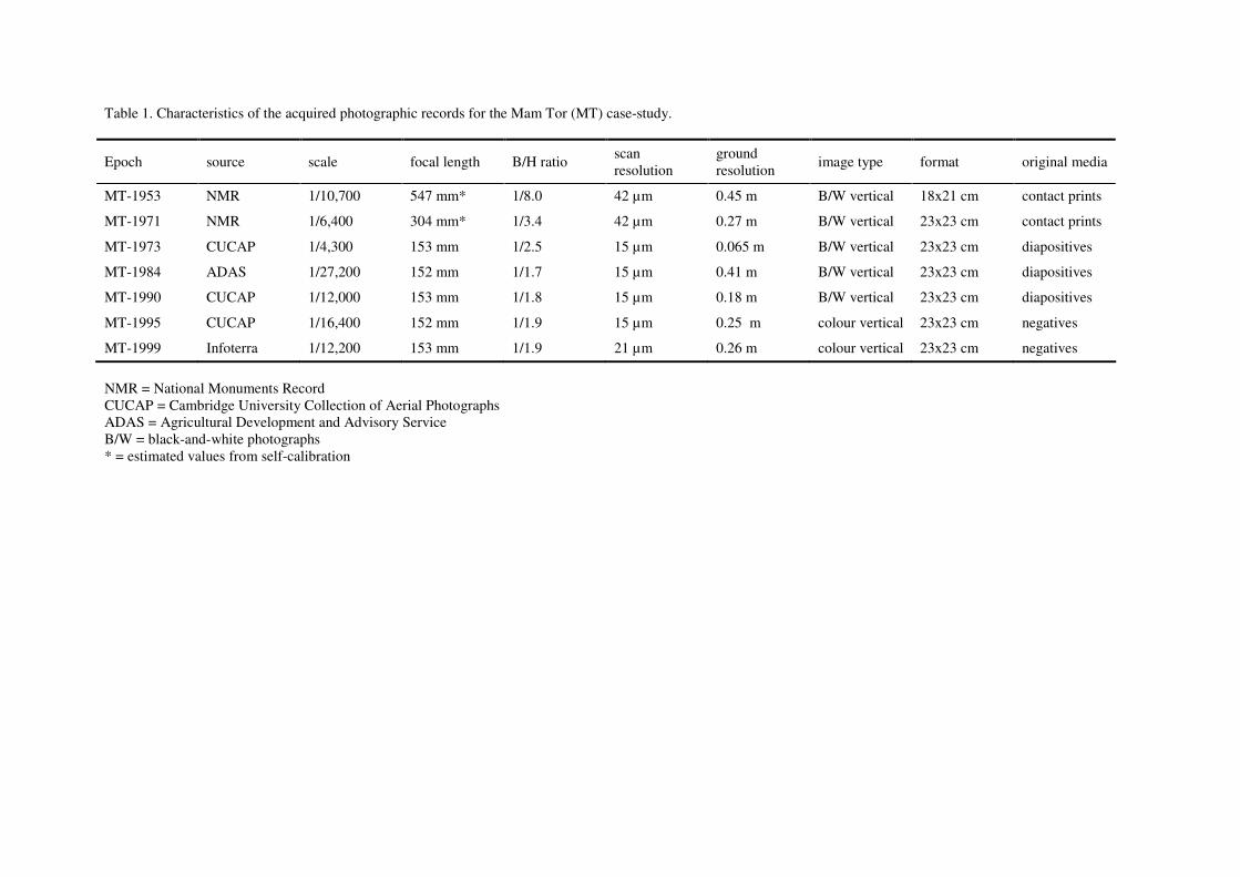
Table 1. Characteristics of the acquired photographic records for the Mam Tor (MT) case-study.

Epoch source scale focal length B/H ratio scan

resolution

ground

resolution image type format original media

MT-1953 NMR 1/10,700 547 mm* 1/8.0 42 µm 0.45 m B/W vertical 18x21 cm contact prints

MT-1971 NMR 1/6,400 304 mm* 1/3.4 42 µm 0.27 m B/W vertical 23x23 cm contact prints

MT-1973 CUCAP 1/4,300 153 mm 1/2.5 15 µm 0.065 m B/W vertical 23x23 cm diapositives

MT-1984 ADAS 1/27,200 152 mm 1/1.7 15 µm 0.41 m B/W vertical 23x23 cm diapositives

MT-1990 CUCAP 1/12,000 153 mm 1/1.8 15 µm 0.18 m B/W vertical 23x23 cm diapositives

MT-1995 CUCAP 1/16,400 152 mm 1/1.9 15 µm 0.25 m colour vertical 23x23 cm negatives

MT-1999 Infoterra 1/12,200 153 mm 1/1.9 21 µm 0.26 m colour vertical 23x23 cm negatives

NMR = National Monuments Record

CUCAP = Cambridge University Collection of Aerial Photographs

ADAS = Agricultural Development and Advisory Service

B/W = black-and-white photographs

* = estimated values from self-calibration

Table 2. Characteristics of the acquired photographic records for the East Pentwyn (EP) case-study.

Epoch source scale focal length B/H ratio scan

resolution

ground

resolution image type format original media

EP-1951 CRAPW 1/9,800 508 mm* 1/6.8 14 µm 0.14 m B/W vertical 18x21 cm diapositives

EP-1955 CRAPW 1/9,200 508 mm* 1/7.6 14 µm 0.13 m B/W vertical 18x21 cm diapositives

EP-1971 Fugro-BKS 1/13,000 153 mm* 1/1.9 14 µm 0.18 m B/W vertical 23x23 cm diapositives

EP-1973 CRAPW 1/8,000 152 mm 1/1.7 16 µm 0.13 m B/W vertical 23x23 cm diapositives

CRAPW = Central Register of Air Photography for Wales

Fugro-BKS = formerly BKS Surveys

B/W = black-and-white photographs * = estimated values from auxiliary data

Table 3. Achieved accuracies of the photogrammetric solutions, assessed by independent checkpoints and expressed in terms of mean error (ME) and standard deviation of

error (SDE).

Epoch number of

checkpoints accuracy of photogrammetric model in object space (m)

X Y Hor Z

ME SDE ME SDE ME SDE ME SDE

MT-1953 4 -0.07 0.63 0.23 1.60 0.24 1.71 -0.42 4.84

MT-1971 5 0.03 0.52 0.29 0.34 0.29 0.62 -0.82 0.99

MT-1973 4 -0.11 0.09 0.20 0.22 0.23 0.24 0.14 0.59

MT-1984 5 -0.30 0.37 0.18 0.40 0.35 0.55 1.17 1.37

MT-1990 6 -0.12 0.25 0.27 0.32 0.29 0.41 0.07 0.45

MT-1995 6 -0.12 0.36 0.04 0.26 0.13 0.44 -0.26 0.49

MT-1999 5 -0.21 0.17 -0.08 0.32 0.22 0.37 0.15 0.88

EP-1951 7 0.76 1.72 0.06 1.21 0.76 2.11 2.99 8.69

EP-1955 4 -0.76 1.34 -0.04 1.08 0.76 1.72 15.91 3.96

EP-1971 5 -0.21 0.20 0.12 0.26 0.24 0.33 -0.38 0.82

EP-1973 2 0.45 1.05 -0.06 0.41 0.46 1.13 1.23 2.07

Table 4. Comparison between expected (RMSE) and observed accuracy (SDE); note that RMSE(X,Y) represents accuracy in either X or Y, whereas RMSE(Hor) is the

summed error of both.

Epoch expected accuracy (m) observed accuracy (m) observed/expected accuracy

RMSE (X, Y) RMSE (Hor) RMSE (Z) SDE (X) SDE (Y) SDE (Hor) SDE (Z) ratio (Hor) ratio (Z)

MT-1953 0.090 0.128 0.719 0.63 1.60 1.71 4.84 13,40 6,73

MT-1971 0.055 0.077 0.183 0.52 0.34 0.62 0.99 8,04 5,42

MT-1973 0.016 0.023 0.034 0.09 0.22 0.24 0.59 10,39 17,33

MT-1984 0.082 0.116 0.139 0.37 0.40 0.55 1.37 4,71 9,82

MT-1990 0.037 0.053 0.066 0.25 0.32 0.41 0.45 7,78 6,81

MT-1995 0.050 0.071 0.094 0.36 0.26 0.44 0.49 6,23 5,17

MT-1999 0.052 0.074 0.098 0.17 0.32 0.37 0.88 4,98 9,01

EP-1951 0.029 0.041 0.187 1.72 1.21 2.11 8.69 50,98 46,51

EP-1955 0.028 0.039 0.196 1.34 1.08 1.72 3.96 44,09 20,18

EP-1971 0.038 0.053 0.070 0.20 0.26 0.33 0.82 6,10 11,68

EP-1973 0.027 0.039 0.045 1.05 0.41 1.13 2.07 28,95 46,45

Table 5. Standard deviations of image measurements of five different objects on the MT-1953 image by six different operators (experts: A1, A2, A3; ‘non-experts’: B1, B2,

B3). Units are in pixels.

Operator

1

Shed corner

2

Farm house

corner

3

Shed corner

4

Intersection of

walls

5

Shed corner

All

(‘within’

operator)

A1 x 0.26 0.26 0.54 0.27 1.22 0.63

y 0.42 0.49 0.29 0.26 1.10 0.60

A2 x 0.33 1.08 0.59 0.56 1.65 0.97

y 0.62 1.41 0.65 0.28 1.64 1.05

A3 x 0.25 0.09 0.41 0.20 0.32 0.28

y 0.31 0.36 0.31 0.18 0.21 0.28

B1 x 0.36 0.71 0.61 0.32 0.82 0.60

y 0.17 0.85 0.49 0.25 0.25 0.47

B2 x 0.18 0.93 0.52 0.51 0.90 0.67

y 0.39 1.36 0.45 0.31 0.92 0.79

B3 x 0.62 1.33 1.00 0.90 1.23 1.05

y 0.57 0.57 0.77 0.65 0.44 0.61

All x 0.99 1.76 1.03 0.54 2.86 1.65

(‘between’ operator) y 0.59 1.69 0.79 0.40 3.60 1.84

Covariance -0.204* -1.679* -0.580* 0.034 -6.700*

* Correlation x-y is significant at the 0.01 level (2-tailed)

Table 6. Standard deviations of image measurements of five different objects on the MT-1973 image by six different operators (experts: A1, A2, A3; ‘non-experts’: B1, B2,

B3). Units are in pixels.

Operator

1

Shed corner

2

Farm house

corner

3

Shed corner

4

Intersection of

walls

5

Shed corner

All

(‘within’

operator)

A1 x 0.86 1.75 0.97 0.61 1.42 1.19

y 1.82 0.94 1.89 0.73 1.70 1.50

A2 x 0.96 1.56 1.28 1.47 3.36 1.92

y 1.37 1.95 1.19 1.40 1.48 1.50

A3 x 1.46 0.47 0.79 0.36 0.65 0.84

y 2.25 0.45 0.47 0.64 0.52 1.11

B1 x 0.67 0.67 0.90 0.29 0.51 0.64

y 1.35 0.45 0.55 0.61 0.32 0.75

B2 x 2.10 1.91 0.98 0.77 2.53 1.79

y 2.99 1.52 0.36 4.54 1.79 2.65

B3 x 0.63 2.44 5.65 0.64 1.32 2.84

y 0.94 4.35 8.66 2.34 1.51 4.53

All x 2.05 15.43 4.33 0.90 9.75 8.45

(‘between’ operator) y 2.85 7.60 4.27 5.25 5.54 5.34

Covariance -4.756* 58.880* -12.833* -2.196* -49.986*

* Correlation x-y is significant at the 0.01 level (2-tailed)

Figure 1. Typical examples of historical photographs used in the case-study of Mam Tor: left image is a RAF

airphoto acquired in 1953, right image was taken by Ordnance Survey in 1971 (© Crown copyright Ordnance

Survey. All rights reserved).These examples clearly illustrate that the available material does not always meet

the ideal qualities for photogrammetric analysis: The RAF image was taken from great height and is hazy, while

both images are rather poor quality scanned contact-prints (North is up).

Figure 2. Horizontal displacement vectors of the Mam Tor landslide, obtained through repeated measurement of

natural surface objects from the 1973 and 1999 image epochs. Background image is an orthophoto created from

the 1999 imagery. The error ellipses represent the 0.05 level of significance, scale of vectors is 15x image scale.

Figure 3. Comparison between expected horizontal accuracy (RMSE) and observed horizontal accuracy (SDE);

the epochs are grouped according to their calibration status.

Figure 4. Relation between ground resolution and observed horizontal accuracy (SDE).

Figure 5. Two of the test points, typically used for ground control in the case-studies. Upper pictures show the

objects in the field: the corner of a farm house (indicated by arrow) and a dry stonewall used as field boundary.

Lower images show the test points on excerpts from the aerial photographs. The point clouds represent all

individual measurements by the six operators. The variance of the measurements ‘within’ and ‘between’

operators is clearly demonstrated by the clustering of point clouds.

Figure 6. The effects of various factors on data accuracy; the categories on top provide the highest achievable

accuracy, decreasing downwards. The scale bar on the right and position of the epochs from this study are an

approximation.