Evaluation of the ACCESS-S1 hindcasts for prediction of ... · evaluation of the access-s1...

Bureau Research Report – 019

Evaluation of the ACCESS-S1 hindcasts for prediction

of Victorian seasonal rainfall

Lim, E.-P., Hendon, H.H., Hudson, D., Zhao, M., Shi, L., Alves O. and Young, G.

October 2016

EVALUATION OF THE ACCESS-S1 HINDCASTS FOR PREDICTION OF VICTORIAN SEASONAL RAINFALL

i

Evaluation of the ACCESS-S1 hindcasts for

prediction of Victorian seasonal rainfall

Lim, E.-P., Hendon, H.H., Hudson, D., Zhao, M., Shi, L., Alves O. and Young, G.

Research and Development Branch, Bureau of Meteorology

Bureau Research Report No. 019

October 2016

National Library of Australia Cataloguing-in-Publication entry

Author: Lim, E.-P., Hendon, H.H., Hudson, D., Zhao, M., Shi, L., Alves O. and Young, G.

Title: Evaluation of the ACCESS-S1 hindcasts for prediction of Victorian seasonal rainfall

ISBN: 978-0-642-70686-7 Series: Bureau Research Report - BRR019


ii

Enquiries should be addressed to: Contact Name: Eun-Pa Lim Bureau of Meteorology GPO Box 1289, Melbourne Victoria 3001, Australia Contact Email: [email protected]

Copyright and Disclaimer

© 2016 Bureau of Meteorology. To the extent permitted by law, all rights are reserved and no part of

this publication covered by copyright may be reproduced or copied in any form or by any means

except with the written permission of the Bureau of Meteorology.

The Bureau of Meteorology advise that the information contained in this publication comprises

general statements based on scientific research. The reader is advised and needs to be aware that such

information may be incomplete or unable to be used in any specific situation. No reliance or actions

must therefore be made on that information without seeking prior expert professional, scientific and

technical advice. To the extent permitted by law and the Bureau of Meteorology (including each of its

employees and consultants) excludes all liability to any person for any consequences, including but

not limited to all losses, damages, costs, expenses and any other compensation, arising directly or

indirectly from using this publication (in part or in whole) and any information or material contained

in it.


iii

Contents Abstract ......................................................................................................................... 1

1. Introduction .......................................................................................................... 2

2. Models, hindcasts and verification data sets ................................................... 3 2.1 ACCESS-S1 ........................................................................................................... 3

2.1.1 Model configuration ................................................................................................. 3 2.1.2 Hindcast initialisation and ensemble generation .................................................... 4

2.2 POAMA .................................................................................................................. 4 2.2.1 Model configuration ................................................................................................. 4 2.2.2 Hindcast initialisation and ensemble generation .................................................... 5

2.3 Verification data and methods ................................................................................ 6

3. Results .................................................................................................................. 7 3.1 Model mean state ................................................................................................... 7

3.2 Prediction of climate indices ................................................................................. 13

3.3 Simulation of teleconnections ............................................................................... 17

3.4 Prediction of Victorian seasonal rainfall ................................................................ 28

4. Concluding Remarks ......................................................................................... 36

5. Acknowledgement ............................................................................................. 37

6. References ......................................................................................................... 37

Appendix A .................................................................................................................. 41


iv

List of Figures

Fig. 1 SST bias in the ensemble mean climatology of ACCESS-S1 (left panels) and POAMA (right panels) relative to Reynolds OI v2 SST analyses at 2 month lead time (LT2). Initialisation time and verification time are shown at the left and right top corners of each plot, respectively. Unit is °C. ............................................................................................................... 8

Fig. 2 Mean sea level pressure (MSLP) bias in the ensemble mean climatology of ACCESS-S1 (left panels) and POAMA (right panels) relative to the ERA-Interim reanalysis at LT2. Initialisation time and verification time are shown at the left and right top corners of each plot, respectively. Unit is hPa. ............................................................................................ 9

Fig. 3 200 hPa level zonal wind bias (shading) in the ensemble mean climatology of ACCESS-S1 (left panels) and POAMA (right panels) relative to the ERA-Interim reanalysis at LT2. Initialisation time and verification time are shown at the left and right top corners of each plot, respectively. Unit is m/s. The climatology of the ERA-Interim 200 hPa level zonal wind is shown with contours. Thick contour line indicates zero and the solid and dashed lines indicate westerlies and easterlies, respectively. The contour interval is 10 m/s. ........................ 10

Fig. 4 Rainfall bias in the ensemble mean climatology of ACCESS-S1 (left panels) and POAMA (right panels) relative to the ERA-Interim reanalysis at LT2. Initialisation time and verification time are shown at the left and right top corners of each plot, respectively. Unit is mm/day. 11

Fig. 5 Mean rainfall in the AWAP analysis (top row), ACCESS-S1 (middle row) and POAMA (bottom row). Forecasts are initialised (a) on the 1st of February and verified in February-April (left column; LT0) and April-June (right column; LT2) and (b) on the 1st of August and verified in August-October (left columns; LT0) and October-December (right panels; LT2). Unit is mm/day. .................................................................................................... 12

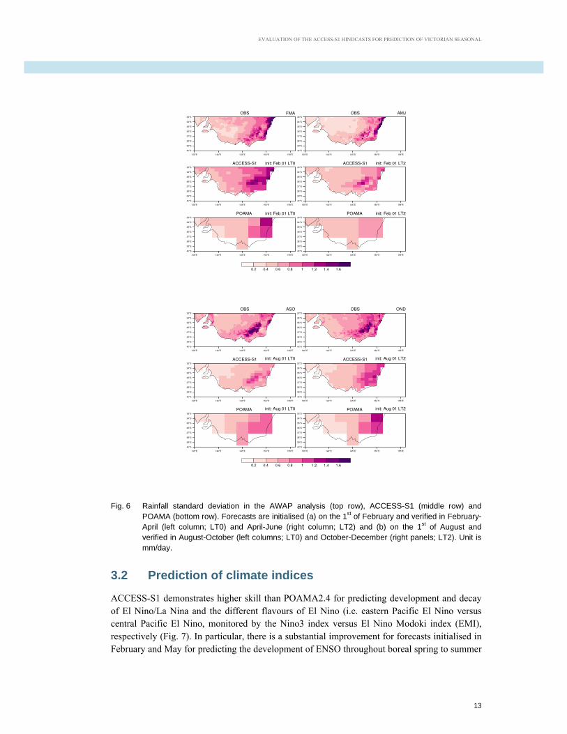
Fig. 6 Rainfall standard deviation in the AWAP analysis (top row), ACCESS-S1 (middle row) and POAMA (bottom row). Forecasts are initialised (a) on the 1st of February and verified in February-April (left column; LT0) and April-June (right column; LT2) and (b) on the 1st of August and verified in August-October (left columns; LT0) and October-December (right panels; LT2). Unit is mm/day. .......................................................................... 13

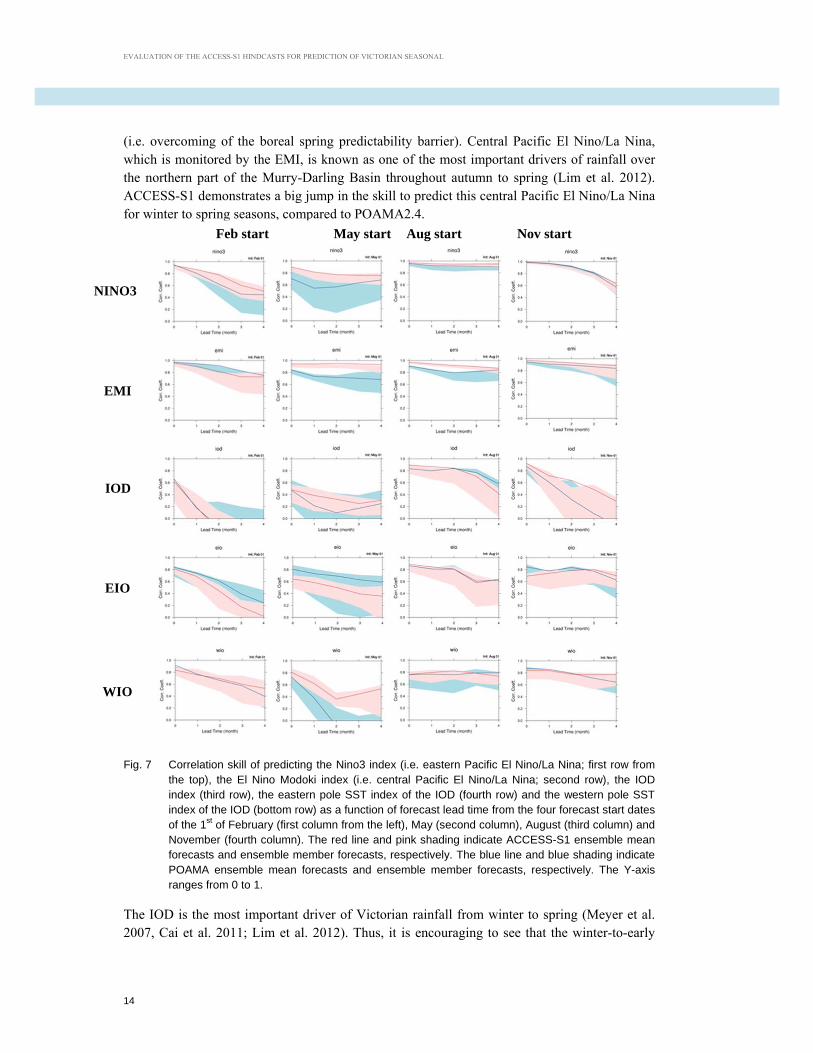
Fig. 7 Correlation skill of predicting the Nino3 index (i.e. eastern Pacific El Nino/La Nina; first row from the top), the El Nino Modoki index (i.e. central Pacific El Nino/La Nina; second row), the IOD index (third row), the eastern pole SST index of the IOD (fourth row) and the western pole SST index of the IOD (bottom row) as a function of forecast lead time from the four forecast start dates of the 1st of February (first column from the left), May (second column), August (third column) and November (fourth column). The red line and pink shading indicate ACCESS-S1 ensemble mean forecasts and ensemble member forecasts, respectively. The blue line and blue shading indicate POAMA ensemble mean forecasts and ensemble member forecasts, respectively. The Y-axis ranges from 0 to 1. ......... 14

Fig. 8 As for Fig. 7, but showing standard deviations of the magnitude of the respective predicted indices. The black dotted line indicates the observed standard deviation of each index. The Y-axis ranges from 0 to 1.8 .......................................................................... 16

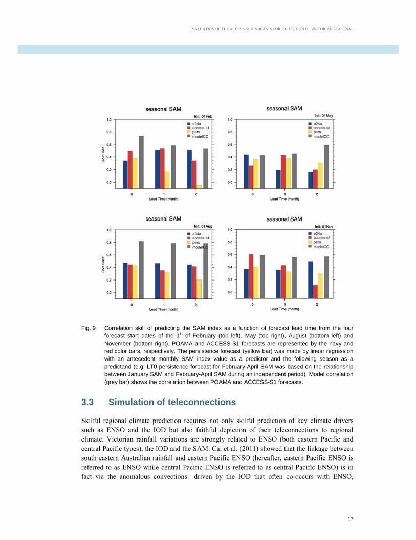
Fig. 9 Correlation skill of predicting the SAM index as a function of forecast lead time from the four forecast start dates of the 1st of February (top left), May (top right), August (bottom left) and November (bottom right). POAMA and ACCESS-S1 forecasts are represented by the navy and red color bars, respectively. The persistence forecast (yellow bar) was made by linear regression with an antecedent monthly SAM index value as a predictor and the following season as a predictand (e.g. LT0 persistence forecast for February-April SAM was based on the relationship between January SAM and February-


v

April SAM during an independent period). Model correlation (grey bar) shows the correlation between POAMA and ACCESS-S1 forecasts. ........................................................................... 17

Fig. 10 Correlation of the Nino3 index respectively with the IOD index (top), the eastern pole SST index of the IOD (middle) and the western pole SST index of the IOD (bottom) in observations (dotted black line), ACCESS-S1 (solid red line indicating the mean of ensemble member correlations), and POAMA (solid blue line indicating the mean of ensemble member correlations). The pink and light blue color shadings indicate ACCESS-S1 and POAMA ensemble member correlations, respectively. Forecasts are initialised on the 1st of May (left) and August (right). ..................................................................................................................... 18

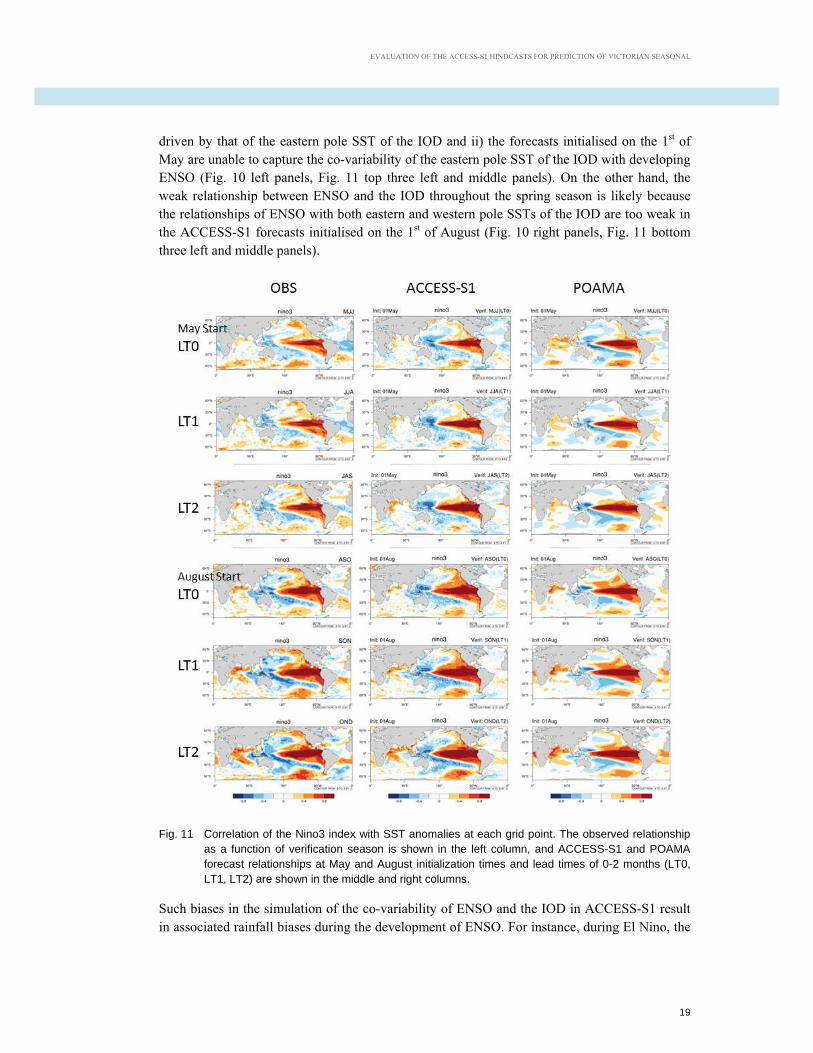
Fig. 11 Correlation of the Nino3 index with SST anomalies at each grid point. The observed relationship as a function of verification season is shown in the left column, and ACCESS-S1 and POAMA forecast relationships at May and August initialization times and lead times of 0-2 months (LT0, LT1, LT2) are shown in the middle and right columns. ............. 19

Fig. 12 As for Fig. 11 except for correlation of the Nino3 index with rainfall anomalies at each grid point. .......................................................................................................................... 21

Fig. 13 Correlation of the IOD index with its eastern pole SST index (top) and western pole SST index (middle) as a function of forecast lead time up to 2 months. The bottom panels show the correlation between the eastern pole SST index and the western pole SST index of the IOD. Forecasts are initialized on the 1st of May (left) and August (right). The red and blue color lines indicate the mean of ensemble member correlations of ACCESS-S1 and POAMA, respectively. The pink and light blue shadings indicate the ensemble member correlations of ACCESS-S1 and POAMA, respectively. The dotted black line indicates the observed correlation. ................................................................................................................. 22

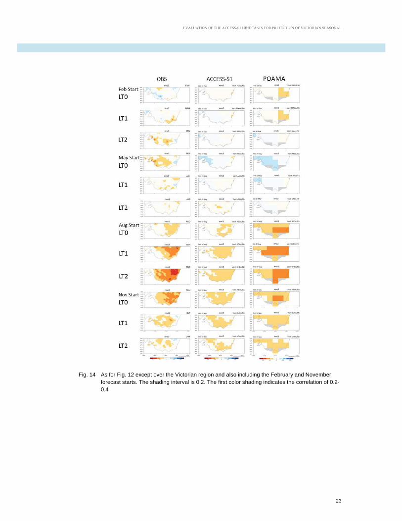
Fig. 14 As for Fig. 12 except over the Victorian region and also including the February and November forecast starts. The shading interval is 0.2. The first color shading indicates the correlation of 0.2-0.4 ............................................................................................................ 23

Fig. 15 As for Fig. 14 except correlation of the IOD with rainfall anomalies at each grid point over the Victorian region. The shading interval is 0.2. The first color shading indicates the correlation of 0.2-0.4. ........................................................................................................... 24

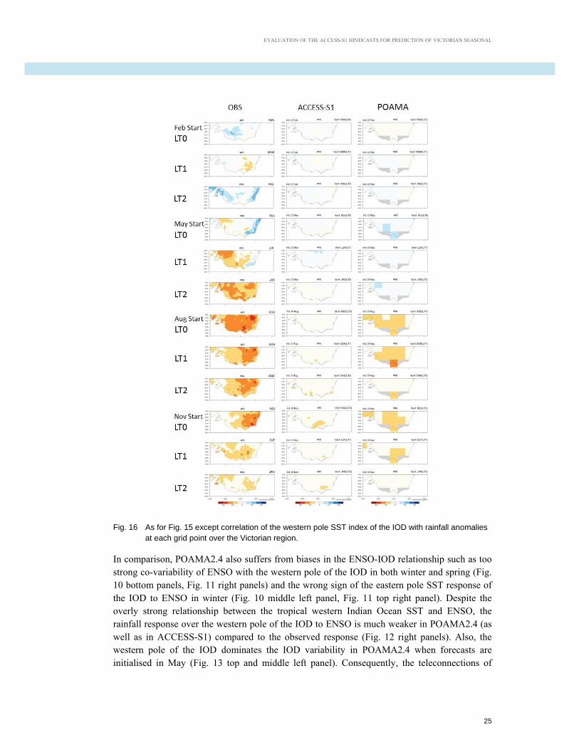
Fig. 16 As for Fig. 15 except correlation of the western pole SST index of the IOD with rainfall anomalies at each grid point over the Victorian region. .................................................. 25

Fig. 17 As for Fig. 15 except correlation of the EMI with rainfall anomalies at each grid point over the Victorian region. The shading interval is 0.2. The first color shading indicates the correlation of 0.2-0.4. ........................................................................................................... 26

Fig. 18 Correlation of the Nino3 index with the SAM index in observations (dotted black line), ACCESS-S1 (solid red line indicating the mean of ensemble member correlations), and POAMA (solid blue line indicating the mean of ensemble member correlations. The pink and light blue color shadings indicate ACCESS-S1 and POAMA ensemble spread of the correlation, respectively. ). Forecasts are initialised on the 1st of August (left) and November (right) and verified for the following three seasons. .................................................................... 27

Fig. 19 As for Fig. 15 except correlation of the SAM index with rainfall anomalies at each grid point over the Victorian region. ................................................................................... 28

Fig. 20 Proportion Correct (PC) of probabilistic forecasts for rainfall being above/below the median threshold at 0 and 3 month lead time (LT0, LT3; e.g. for forecasts initialized on 1st February the LT0 forecast verifies in FMA and the LT3 in MJJ). PC of the climatological forecast is 0.5, and PC of ACCESS-S1 and POAMA forecasts being greater than 0.55, which is shown with color shading, is considered to be skillful. The shading interval is 0.1 from 0.55. .............................................................................................................................. 30


vi

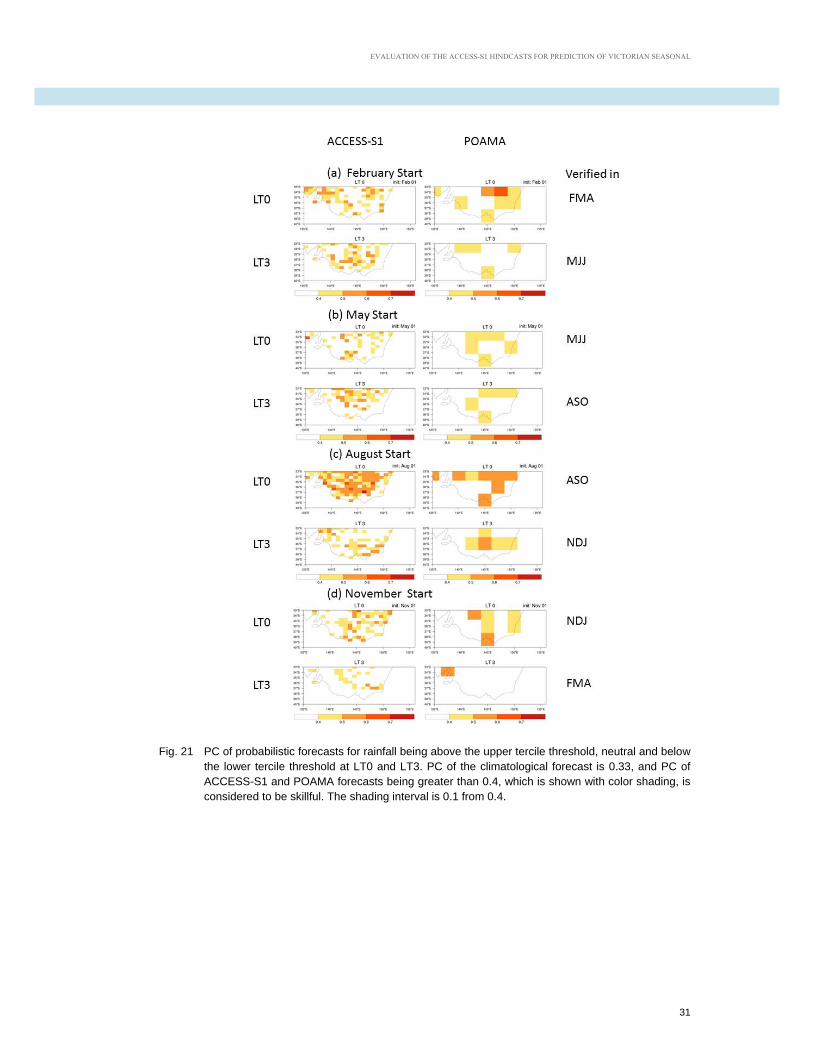
Fig. 21 PC of probabilistic forecasts for rainfall being above the upper tercile threshold, neutral and below the lower tercile threshold at LT0 and LT3. PC of the climatological forecast is 0.33, and PC of ACCESS-S1 and POAMA forecasts being greater than 0.4, which is shown with color shading, is considered to be skillful. The shading interval is 0.1 from 0.4. .. 31

Fig. 22 PC of probabilistic forecasts for rainfall being above the top quintile threshold and below the bottom quintile threshold at LT0 and LT3. PC of the climatological forecast is 0.2, and PC of ACCESS-S1 and POAMA forecasts being greater than 0.3, which is shown with color shading, is considered to be skillful. The shading interval is 0.1 from 0.3. ................. 32

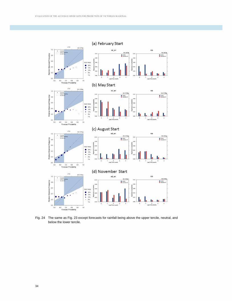
Fig. 23 (left column) reliability diagram of probabilistic forecasts of ACCESS-S1 for rainfall being above/below the median at lead time 0. The diagonal line indicates the perfect reliability, and the blue shading indicates where forecasts are more reliable than the climatological forecast. The size of dots represents the number of forecasts in respective probability bins. (middle column) reliability error (i.e. the average distance of the forecast dots in the left figure from the perfect reliability; lower number is better) of probabilistic forecasts of ACCESS-S1 (red bar) and POAMA (navy bar) as a function of forecast lead time 0 to 4 months (X-axis). The Y-axis ranges from 0 to 0.1. (right column) the same as the middle column except it shows resolution (i.e. the average distance of the forecast dots from the climatological forecast; high number is better) ..................................................................... 33

Fig. 24 The same as Fig. 23 except forecasts for rainfall being above the upper tercile, neutral, and below the lower tercile. ........................................................................................... 34

Fig. 25 The same as Fig. 23 except forecasts being above the top quintile threshold and below the bottom quintile threshold. .................................................................................... 35

EVALUATION OF THE ACCESS-S1 HINDCASTS FOR PREDICTION OF VICTORIAN SEASONAL

1

ABSTRACT

In 2015 the Bureau of Meteorology (BoM) made a major strategic decision to advance its seasonal prediction capability, and so, BoM has been developing a new seasonal prediction system, called ACCESS-S1 (the Australian Community Climate and Earth-System Simulator-Seasonal prediction system). ACCESS-S1 built upon the latest climate model Global Seasonal forecast system version 5 using the Global Coupled configuration 2 (GloSea5-GC2) from the UK Met Office (UKMO) along with locally developed system enhancements. The ACCESS-S1 system is planned to become operational, replacing the BoM’s current operational system POAMA2 by mid-2017.

The UKMO's GloSea5-GC2 includes a number of state-of-the-art features compared to POAMA2, such as substantially higher horizontal and vertical resolution, improved model physics and parameterization, a multi-level land surface model, and an interactive multi-level sea-ice model.

Using a locally developed ensemble generation scheme, 22 member ensemble hindcasts initialised on the 25th of January, April, July and October and on the 1st of February, May, August and November have been generated for the period 1990-2012 from the ACCESS-S1 system. In this report we assessed the performance of ACCESS-S1 in simulating the climate mean states, predicting large-scale climate drivers such as ENSO, IOD and SAM and predicting Victorian climate.

Compared with the POAMA2, ACCESS-S1 demonstrates significantly reduced mean climate bias globally and over Australia, including Victoria. Also, the large-scale climate modes such as ENSO, IOD and SAM are better predicted by ACCESS-S1. Importantly, ACCESS-S1 demonstrates improved skill in predicting Victorian rainfall for late autumn, winter and spring at lead times up to 3 months - especially in predicting extreme rainfall events with greatly improved spatial detail. However, there is still a large scope for improvement, including overestimation of the magnitude of ENSO and IOD and underestimation of the teleconnection strength of ENSO, IOD and SAM to Victorian rainfall.


2

1. INTRODUCTION

The Bureau of Meteorology is developing a new seasonal prediction system, called ACCESS-S1 (the Australian Community Climate and Earth-System Simulator-Seasonal prediction system), that will use the latest climate model Global Coupled configuration version 2 (GC2) from the UK Met Office (UKMO) along with locally developed system enhancements. The ACCESS-S1 system is planned to become operational by the end of 2016, replacing the BoM’s current operational system POAMA2.4 by mid-2017.

The UKMO's global coupled climate model GloSea5-GC2 (Global Seasonal forecast system version 5 using the Global Coupled configuration 2) includes a number of state-of-the-art features compared to POAMA2.4, such as substantially higher horizontal and vertical resolution, improved model physics and parameterization, an multi-level land surface model, and an interactive multi-level sea-ice model. For instance, GloSea5-GC2 is run on ~60 km horizontal resolution in the atmosphere, which resolves details of orography and topography such as the Dividing Range and coastal areas and resolves southern Victoria and Tasmania; and uses 85 vertical levels with a fully resolved stratosphere and top at 0.1 hPa. In comparison, POAMA has ~250 km horizontal resolution and 17 vertical levels in the atmosphere with top at 9.6 hPa and only 5 levels about 200 hPa level in the stratosphere. The ocean model (NEMO) also has much higher horizontal (0.25° globally) and vertical resolution (75 levels) than POAMA (0.5° tropics to 1.5° at the poles and 25 vertical levels), which better resolves tropical instability waves, mixed layer processes, coastal current and upwelling zones, and subsurface processes associated with the El Nino-Southern Oscillation (ENSO). Also, GC2 includes climate forcing of greenhouse gases with realistic time-variation, while it is held constant at the level of 1985 in POAMA.

Previous studies have assessed the hindcast skill of an earlier version of GloSea5 (GloSea5-Global Atmosphere configuration version 3 (GA3)) over the period 1996-2009 (e.g. MacLachlan et al. 2014, Hendon et al. 2015, Zou et al. 2015). They showed that GloSea5-GA3 was more skilful in depicting the climatological mean states of sea surface temperature (SST), global rainfall and Australian temperature and rainfall than POAMA2.4. Also, the large-scale climate drivers such as ENSO, the Indian Ocean Dipole mode (IOD), the Southern Annular Mode (SAM) and the Madden-Julian Oscillation (MJO) and short-lead Australian sub-seasonal climate were better predicted by GloSea5-GA3 than by POAMA2.4. Recently, Shi et al. (2016a,b) evaluated the 3 member ensemble hindcasts generated from GloSea5-GC2 for the period of 1996-2009 and reported that GloSea5-GC2 is clearly more skilful than POAMA2.4 for the first two fortnights of the forecast (i.e. weeks 1+2, weeks 2+3) at the short lead times. However, skill to predict Australian maximum temperature was found to be lower in GloSea5-GC2 than POAMA. While these results are helpful in understanding the basic skill we expect to achieve with ACCESS-S1, confidence in the results is somewhat limited by the relatively small ensemble size and short hindcast period of GloSea5-GC2. Also, no assessment of the skill of GloSea5-GC2 has been conducted specifically for predicting Victorian climate.


3

The final version of the ACCESS-S1 system has been configured and tested, including a locally developed ensemble generation scheme, and production of the hindcasts for the period 1990-2012 has commenced. The full hindcast set will comprise an 11 member ensemble initialised four times every month for the period 1990-2012. As of mid-May 2016, hindcasts initialised on the 1st February, 1st May, 1st August and 1st November have been completed. In this report we assess the skill of these ACCESS-S1 hindcasts for ENSO, the IOD and the SAM, which are important drivers of Australian seasonal climate, and for Victorian seasonal rainfall and temperature in comparison to the skill of POAMA2.4.

2. MODELS, HINDCASTS AND VERIFICATION DATA SETS

2.1 ACCESS-S1

2.1.1 Model configuration

GloSea5-GC2/ACCESS-S1 consists of the following components (Williams et al. 2015):

Atmosphere: the Unified Model (UM) Global Atmosphere version 6 (GA6) (Williams et al. 2014)

Land surface: the Joint UK Land Environment Simulator (JULES) Global Land version 6 (GL6; Best et al. 2011)

Ocean: the NEMO global ocean model Global Ocean version 5 (GO5; Megann et al. 2014)

Sea-ice: the Los Alamos Sea Ice Model (CICE) Global Sea-Ice version 6 (GSI6; Rae et al. 2014)

The dynamical core of the UM atmospheric model (called Even Newer Dynamics for General atmospheric modelling of the environment – ENDGame) uses an iterative semi-implicit semi-Lagrangian discretization to solve the fully compressible, non-hydrostatic atmospheric equations of motion (http://www.metoffice.gov.uk/research/areas/dynamics/endgame). The UM also uses the stochastic physics scheme called Stochastic Kinetic Energy Backscatter v2 (SKEB2; Bowler et al. 2009) to represent unresolved processes and provide small grid-level perturbations during the model integration (MacLachlan et al. 2015). Climate forcing of greenhouse gases is set to observed values up to the year 2005 and to follow the IPCC Radiative Concentration Pathway 4.5 scenario post-2005. Other aerosols and ozone are set to the climatological values with a seasonal cycle (MacLachlan et al. 2015). Williams et al. (2015) report that relative to GloSea5-GA3, GloSea5-GC2 has numerous changes, including major upgrades of component models, revisions to the existing parametrization schemes and implementation of a new cloud scheme.

The UM with 85 vertical levels and JULES with 4 soil levels are tightly coupled on the same horizontal grid of N216 (~60km in the midlatitudes). Similarly, the NEMO ocean model with 75 vertical levels and the CICE sea-ice model with 5 thickness categories are strongly coupled on the same horizontal grid of 0.25° (~27 km on the equator). The atmosphere/land and the


4

ocean/sea-ice are coupled every 3 hours by Ocean Atmosphere Sea Ice Soil (OASIS) coupler version 3 (Williams et al. 2015).

2.1.2 Hindcast initialisation and ensemble generation

ACCESS-S1 hindcasts are initialised on the 1st, 9th, 17th and 25th of each month over the period 1990-2012. ERA-Interim reanalysis data are used to initialise the atmosphere component model and land temperatures (MacLachlan et al. 2015). The soil moisture is initialised with monthly climatology of a land surface reanalysis using the JULES forced with the Intergrated Project Water and Global Change Forcing Data methodology applied to ERA-Interim data (Weedon et al. 2011, MacLachlan et al. 2015) but with the climatology bias corrected to match the available climatology derived from atmospheric initialisation routinely run at the UKMO for numerical weather prediction (MacLachlan et al. 2015).

For the ACCESS-S1 hindacasts, the ocean and sea-ice models are initialized with the GloSea5 Ocean and Sea Ice Analysis that is produced by the UKMO FOAM system (Blockley et al. 2013). . This ocean analysis is produced from the NEMO 3-dimentional variational ocean data assimilation system (NEMOVAR) forced by ERA-Interim reanalysis at UKMO and using the same version of the NEMO ocean model as in GC2. NEMOVAR assimilates both satellite and in situ observations of SST, sea level anomaly satellite data, sub-surface temperature and salinity profiles, and satellite observations of sea-ice concentration (MacLachlan et al. 2015).

Only a single set of atmosphere-ocean initial conditions is provided from the ERA-Interim reanalyses on the four different initialisation times of each month for 1990-2012. In order to sample observational uncertainty in the atmospheric initial condition, which is especially important to produce sufficient forecast spread in the first month of the forecasts, a perturbation generation technique was developed (see details in Appendix A).Ten additional ensemble members are then generated by perturbing the atmosphericstate with this approach..

The 11 member ensemble hindcasts initialised on the 1st of February, May, August and November for the period 1990-2011 are analysed in this report.

2.2 POAMA

2.2.1 Model configuration

POAMA version 2.4 is the BoM’s current operational sub-seasonal to seasonal climate forecast system. POAMA2.4 is based on a coupled ocean-atmosphere model that consists of the Bureau’s Atmospheric Model version 3 (BAM3; Colman et al. 2005) and the Australian Community Ocean Model version 2 (ACOM2) (Schiller et al., 1997; 2002). ACOM2 is based on the Geophysical Fluid Dynamics Laboratory Modular Ocean Model (MOM version 2). The atmosphere model uses the spectral transform technique, with T47 truncation (roughly ~250 km horizontal resolution) with 17 vertical levels and top at 9.6 hPa (these levels do not resolve the stratosphere; Shi et al. 2016b). The land surface component is a simple bucket model for soil moisture (Manabe and Holloway 1975) and has three soil levels for temperature. The ocean grid


5

resolution is 2° in the zonal direction and 0.5° in the meridional direction at the equator, which gradually increases to 1.5° near the poles. The ocean model has 25 vertical levels. The atmosphere and ocean models are coupled daily by OASIS (Valcke et al., 2000). POAMA2.4 has no sea-ice model. Greenhouse gas forcing is not time-varying and is fixed to 345 ppm (representative of the mid-1980s), and ozone concentration and sea-ice extents are set to the respective climatological values (the climatology of sea-ice extents was computed over the period 1981-2000; personal communication with Dr Guomin Wang).

2.2.2 Hindcast initialisation and ensemble generation

POAMA hindcasts are initialised from observed atmospheric and oceanic states. Atmosphere and land initial conditions are generated from the Atmosphere-Land Initialisation scheme (ALI; Hudson et al., 2011). ALI nudges the model atmospheric fields (u, v, T, and q) towards an existing analysis of observation every 6 hours. For the period 1980-2002, the ERA-40 reanalyses (Uppala et al. 2005) are used, and for the period 2003-onward the analyses from the BoM’s operational numerical weather prediction are used. Through this nudging process the land surface is realistically initialised in response to the surface fluxes generated in the atmosphere. Ocean initial conditions are generated from the POAMA Ensemble Ocean Data Assimilation System (PEODAS; Yin et al., 2011). In situ temperature and salinity observations are assimilated to a central run of the ocean model that is forced by re-analysis surface fluxes. An ensemble of ocean states is then generated by perturbing the surface fluxes within a possible range of observational errors on intra-seasonal time scales. This ensemble of ocean states is used to compute the background error covariances for temperature, salinity and currents. Using these background error covariances, observed data are assimilated to the central run. After each analysis cycle (3 days), the ensemble members are nudged toward the analysis from the central run. The resultant ensemble of ocean conditions is used to initialise the ensemble of seasonal forecasts.

To address model uncertainty, POAMA2.4 uses a pseudo multi-model ensemble strategy using three different versions of the atmospheric model. A 33-member ensemble, generated in ‘burst’ mode (i.e. all initial conditions are valid for the same date and time, with no time lag), is run for each start date. The 33-member ensemble comprises an 11-member ensemble for each of the three model versions. Perturbations to the atmosphere and ocean initial conditions are produced by a coupled-model breeding scheme (Hudson et al. 2013). POAMA hindcasts are available for the period 1981-2014.

To make a fair comparison to the ACCESS-S1 hindcasts, we use 11-member ensemble hindcasts generated from one version of POAMA (e24a) for the period 1990-2011. This relatively small ensemble size and the short hindcast period are caveats of this evaluation, which should be borne in mind when results are interpreted.


6

2.3 Verification data and methods

Apart from examining the models’ ability to simulate global mean climate, we use forecast and observed anomalies in estimating the skill of predicting global and regional climate variability. This is done by removing the respective forecast and observed climatologies.

Forecasts for SST are verified against Reynolds OI v2 SST analysis. For ENSO, we compute the Nino3 index and El Nino Modoki index (EMI) as follows:

Nino3 index = (5°S-5°N, 210°-270°E)

EMI = (10°S-10°N, 165°-220°E) - 0.5* (15°S-5°N, 250°-290°E) - 0.5* (10°S-20°N, 125°-145°E)

where the overbar indicates the spatial average over the domain shown in parentheses.

Regarding the IOD, we compute the IOD index (also called Dipole Mode Index) but also examine the eastern pole and western pole of the IOD separately (i.e. EIO and WIO).

WIO index = (10°S-10°N, 50°-70°E)

EIO index = (10°S-0°N, 90°-110°E)

IOD index = WIO - EIO

For global atmospheric variables, forecasts are verified against the ERA-Interim reanalysis. We assess the skill to predict the seasonal SAM by computing the SAM index following Gong and Wang (1999)’s definition, which is the difference of normalised mean sea level pressure (MSLP) between 40°S and 65°S:

SAM index = [MSLP]40°S/σ[MSLP]40°S - [MSLP]65°S/σ[MSLP]65°S

where σ indicates standard deviation.

Forecasts for seasonal mean of Victorian rainfall and daily maximum and minimum temperature are verified against the AWAP monthly rainfall and temperature analysis (Jones et al. 2009). In this report, we look at proportion correct (also known as percent consistent score or forecast accuracy) of probabilistic forecasts for rainfall and temperature being above/below the median, above the upper tercile/below the lower tercile/neutral and above the top quintile/below the bottom quintile thresholds. Also, reliability error and resolution of probabilistic forecasts are examined. Calculations of Proportion Correct, reliability error and resolution are as below (also see Wilks 2005):

Proportion Correct = number of correct forecasts for the occurrence and non-occurrence of an event divided by the total number of forecasts


7

Reliability error = ∑ , where n is the total number of forecasts, N is the

number of forecasts in probability category i, Yi is the probability of i-th category and

is the mean of relative observed frequency when forecasts in the i-th category are issued.

Resolution = ∑ , where is the mean of

Larger values of Proportion Correct and forecast resolution indicate better forecast skill and quality, while larger values of forecast reliability error indicate the opposite.

3. RESULTS

3.1 Model mean state

A cold SST bias over much of the globe, which is a common feature in climate models, is pronounced in POAMA2.4, appearing soon after initialisation (Fig. 1). This cold SST bias is substantially alleviated in ACCESS-S1, which is attributed to the much updated atmosphere and ocean models in GC2 (Williams et al. 2015). The warm SST bias in the eastern Pacific is also substantially reduced, and the Southern Ocean warm bias appearing in the austral warm seasons off the Antarctic coast is less severe in ACCESS-S1 compared to POAMA2.4. Williams et al. (2015) attributed this Southern Ocean warm bias to the atmosphere heat flux biases and turbulent flux errors.

As a result of overall reduced SST bias, mean circulations at the surface and aloft are much better captured in ACCESS-S1 compared to POAMA2.4 (Figs 2 and 3). For instance, POAMA2.4 suffers from cold bias everywhere except along the west coast of North and South America (Fig. 1 right panels), which causes the model’s mean circulation to be somewhat El Nino-like in the tropical Pacific and to be somewhat negative SAM-like in the extratropics (Fig. 2 right panels). The equatorward displacement of the eddy-driven jet together with a poleward displacement of the subtropical jet associated with the negative SAM-like circulation bias in POAMA2.4 is not as pronounced in ACCESS-S1 (Figs 2,3 left panels).

However, in ACCESS-S1, the equatorial eastern Pacific SST is much colder than observed and so are the eastern Indian Ocean to the Maritime Continent region and the equatorial Atlantic SST. These cold SST biases lead to dry biases in the equatorial regions in most seasons and in the Maritime Continent region in winter and spring, which are the important seasons for the development of the IOD (Figs 1,4). On the other hand, ACCESS-S1 has wet bias in the central-west Indian Ocean in spring to summer. The dry bias in the Maritime Continent and the wet bias in the central Indian Ocean, which resemble the pattern of rainfall anomalies during the positive phase of the IOD, are likely to play deleterious roles for prediction of the IOD and associated teleconnection to the south-eastern Australian (SEA) region (33-40°S, 135-156°E). Detailed investigation on how the mean SST and rainfall biases of ACCESS-S1 impact the model’s performance in predicting ENSO and the IOD is yet to be carried out.


8

Fig. 1 SST bias in the ensemble mean climatology of ACCESS-S1 (left panels) and POAMA (right panels) relative to Reynolds OI v2 SST analyses at 2 month lead time (LT2). Initialisation time and verification time are shown at the left and right top corners of each plot, respectively. Unit is °C.


9

Fig. 2 Mean sea level pressure (MSLP) bias in the ensemble mean climatology of ACCESS-S1 (left panels) and POAMA (right panels) relative to the ERA-Interim reanalysis at LT2. Initialisation time and verification time are shown at the left and right top corners of each plot, respectively. Unit is hPa.


10

Fig. 3 200 hPa level zonal wind bias (shading) in the ensemble mean climatology of

ACCESS-S1 (left panels) and POAMA (right panels) relative to the ERA-Interim reanalysis at LT2. Initialisation time and verification time are shown at the left and right top corners of each plot, respectively. Unit is m/s. The climatology of the ERA-Interim 200 hPa level zonal wind is shown with contours. Thick contour line indicates zero and the solid and dashed lines indicate westerlies and easterlies, respectively. The contour interval is 10 m/s.


11

Fig. 4 Rainfall bias in the ensemble mean climatology of ACCESS-S1 (left panels) and POAMA (right panels) relative to the ERA-Interim reanalysis at LT2. Initialisation time and verification time are shown at the left and right top corners of each plot, respectively. Unit is mm/day.


12

For SEA rainfall, the spatial detail of the mean rainfall is skilfully reproduced in ACCESS-S1, and is a significant improvement over POAMA (Fig. 5). For example, the mean rainfall and large rainfall variability on the east and west sides of the Great Dividing Range are well captured by ACCESS-S1 (Figs 5,6). Also, the mean rainfall and large rainfall variability over Gippsland and South West, which are districts that POAMA2.4 could not resolve, are skilfully simulated in ACCESS-S1. Seasonal cycles of mean rainfall and variability appear to be better simulated in ACCESS-S1 compared to POAMA2.4 (i.e. left columns compared to the right columns of Figs 5 and 6).

(a)

(b)

Fig. 5 Mean rainfall in the AWAP analysis (top row), ACCESS-S1 (middle row) and POAMA (bottom row). Forecasts are initialised (a) on the 1st of February and verified in February-April (left column; LT0) and April-June (right column; LT2) and (b) on the 1st of August and verified in August-October (left columns; LT0) and October-December (right panels; LT2). Unit is mm/day.


13

(a)

(b)

Fig. 6 Rainfall standard deviation in the AWAP analysis (top row), ACCESS-S1 (middle row) and POAMA (bottom row). Forecasts are initialised (a) on the 1st of February and verified in February-April (left column; LT0) and April-June (right column; LT2) and (b) on the 1st of August and verified in August-October (left columns; LT0) and October-December (right panels; LT2). Unit is mm/day.

3.2 Prediction of climate indices

ACCESS-S1 demonstrates higher skill than POAMA2.4 for predicting development and decay of El Nino/La Nina and the different flavours of El Nino (i.e. eastern Pacific El Nino versus central Pacific El Nino, monitored by the Nino3 index versus El Nino Modoki index (EMI), respectively (Fig. 7). In particular, there is a substantial improvement for forecasts initialised in February and May for predicting the development of ENSO throughout boreal spring to summer


14

(i.e. overcoming of the boreal spring predictability barrier). Central Pacific El Nino/La Nina, which is monitored by the EMI, is known as one of the most important drivers of rainfall over the northern part of the Murry-Darling Basin throughout autumn to spring (Lim et al. 2012). ACCESS-S1 demonstrates a big jump in the skill to predict this central Pacific El Nino/La Nina for winter to spring seasons, compared to POAMA2.4.

Fig. 7 Correlation skill of predicting the Nino3 index (i.e. eastern Pacific El Nino/La Nina; first row from the top), the El Nino Modoki index (i.e. central Pacific El Nino/La Nina; second row), the IOD index (third row), the eastern pole SST index of the IOD (fourth row) and the western pole SST index of the IOD (bottom row) as a function of forecast lead time from the four forecast start dates of the 1st of February (first column from the left), May (second column), August (third column) and November (fourth column). The red line and pink shading indicate ACCESS-S1 ensemble mean forecasts and ensemble member forecasts, respectively. The blue line and blue shading indicate POAMA ensemble mean forecasts and ensemble member forecasts, respectively. The Y-axis ranges from 0 to 1.

The IOD is the most important driver of Victorian rainfall from winter to spring (Meyer et al. 2007, Cai et al. 2011; Lim et al. 2012). Thus, it is encouraging to see that the winter-to-early

NINO3

EMI

IOD

EIO

WIO

Feb start May start Aug start Nov start


15

spring IOD is better predicted by ACCESS-S1. In particular, the substantial improved prediction of the IOD initialised on the 1st of May appears to mainly stem from improved skill to predict the tropical western Indian Ocean. Improved skill in the western Indian Ocean presumably derives from improved prediction of eastern Pacific ENSO because tropical western Indian Ocean SST variations are largely a remote response to El Nino in the Pacific. However, even with this improvement made by ACCESS-S1, the skill for predicting the IOD from May initial conditions is not high, likely due to inherent limits of predictability of the IOD (Shi et al. 2012) and the reduced predictability of the IOD post-2000 (Lim et al. 2016).

While ACCESS-S1 performs better in predicting the occurrence of eastern Pacific and central Pacific ENSO and the IOD compared to POAMA2.4, ACCESS-S1 tends to predict ENSO and the IOD with too strong amplitudes (Fig. 8). For instance, the standard deviation of the Nino3 SST is 0.2°-0.6°C larger than those of the observed and from POAMA2.4. Also, the amplitude of the eastern pole of the IOD is much too large in ACCESS-S1 for forecasts initialised in May, which results in IOD forecasts that are too strong for the following winter-spring seasons.

The positive phase of SAM is characterized by poleward shifts of the eddy-driven jet and associated midlatitude storm track, with nearly zonally symmetric high and low pressure anomalies across the Southern Hemisphere midlatitudes and high latitudes, respectively. Hendon et al. (2007) showed that during the positive phase of the SAM, Victoria tends to receive less rainfall in winter but more rainfall in spring/summer. Both POAMA2.4 and ACCESS-S1 demonstrate moderate skill to predict seasonal SAM (Fig. 9). Our analysis reveals that SAM is better predicted by ACCESS-S1 than POAMA at short lead times (LT) of 0-1 months for most of the seasons, except for predictions for spring (September-October-November; SON) when forecasts are initialised in August and predictions for early winter (May-June-July; MJJ) when forecasts are initialised in May. It is interesting to note that SAM forecasts from POAMA2.4 and ACCESS-S1 are much more similar to each other than to the observed SAM (Fig. 9, grey bar), which might imply high potential predictability of seasonal SAM that we have not been previously aware of. Or, perhaps this indicates that the models are responding similarly to some source of forcing but are then jointly deficient for some other source of predictability or noise. It will be interesting to investigate in a future study if there exists some source of predictability of the seasonal SAM other than ENSO or if the high correlation between the models is merely reflecting a common model bias.


16

Fig. 8 As for Fig. 7, but showing standard deviations of the magnitude of the respective predicted indices. The black dotted line indicates the observed standard deviation of each index. The Y-axis ranges from 0 to 1.8

NINO3

EMI

IOD

EIO

WIO

Feb start May start Aug start Nov start


17

Fig. 9 Correlation skill of predicting the SAM index as a function of forecast lead time from the four forecast start dates of the 1st of February (top left), May (top right), August (bottom left) and November (bottom right). POAMA and ACCESS-S1 forecasts are represented by the navy and red color bars, respectively. The persistence forecast (yellow bar) was made by linear regression with an antecedent monthly SAM index value as a predictor and the following season as a predictand (e.g. LT0 persistence forecast for February-April SAM was based on the relationship between January SAM and February-April SAM during an independent period). Model correlation (grey bar) shows the correlation between POAMA and ACCESS-S1 forecasts.

3.3 Simulation of teleconnections

Skilful regional climate prediction requires not only skilful prediction of key climate drivers such as ENSO and the IOD but also faithful depiction of their teleconnections to regional climate. Victorian rainfall variations are strongly related to ENSO (both eastern Pacific and central Pacific types), the IOD and the SAM. Cai et al. (2011) showed that the linkage between south eastern Australian rainfall and eastern Pacific ENSO (hereafter, eastern Pacific ENSO is referred to as ENSO while central Pacific ENSO is referred to as central Pacific ENSO) is in fact via the anomalous convections driven by the IOD that often co-occurs with ENSO,


18

especially in spring. Hendon et al. (2014) and Lim and Hendon (2015) revealed that the seasonal variation of the SAM has a moderate relationship with ENSO in the austral warm seasons, and concurrence of La Nina and high SAM (or El Nino and low SAM) can result in extreme climate conditions over eastern Australia. Thus, correct simulation of the ENSO-IOD and ENSO-SAM relationships and the relationships of Victorian rainfall with ENSO, IOD and SAM are crucial to make skilful forecasts of Victorian rainfall.

Fig. 10 Correlation of the Nino3 index respectively with the IOD index (top), the eastern pole SST index of the IOD (middle) and the western pole SST index of the IOD (bottom) in observations (dotted black line), ACCESS-S1 (solid red line indicating the mean of ensemble member correlations), and POAMA (solid blue line indicating the mean of ensemble member correlations). The pink and light blue color shadings indicate ACCESS-S1 and POAMA ensemble member correlations, respectively. Forecasts are initialised on the 1st of May (left) and August (right).

The relationship between ENSO and the IOD in winter and spring is simulated to be weaker than observed in ACCESS-S1 (Fig. 10 top panels). This weak relationship during winter in ACCESS-S1 is likely because of two factors: i) forecast variability of the IOD is dominantly


19

driven by that of the eastern pole SST of the IOD and ii) the forecasts initialised on the 1st of May are unable to capture the co-variability of the eastern pole SST of the IOD with developing ENSO (Fig. 10 left panels, Fig. 11 top three left and middle panels). On the other hand, the weak relationship between ENSO and the IOD throughout the spring season is likely because the relationships of ENSO with both eastern and western pole SSTs of the IOD are too weak in the ACCESS-S1 forecasts initialised on the 1st of August (Fig. 10 right panels, Fig. 11 bottom three left and middle panels).

Fig. 11 Correlation of the Nino3 index with SST anomalies at each grid point. The observed relationship as a function of verification season is shown in the left column, and ACCESS-S1 and POAMA forecast relationships at May and August initialization times and lead times of 0-2 months (LT0, LT1, LT2) are shown in the middle and right columns.

Such biases in the simulation of the co-variability of ENSO and the IOD in ACCESS-S1 result in associated rainfall biases during the development of ENSO. For instance, during El Nino, the


20

observed dry anomaly over the tropical eastern Indian Ocean south of Sumatra is absent in the ACCESS-S1 forecasts initialised in May for the following winter seasons, and the wet anomaly over the tropical western Indian Ocean during El Nino is weak in the ACCESS-S1 forecasts initialised in August for the following spring seasons (Fig. 12 left and middle panels). Furthermore, the pattern of the dry anomaly over the tropical eastern Indian Ocean associated with El Nino is meridionally too narrow and westward shifted compared to reality, missing the SST response off the north west coast of Australia for the spring forecasts initialised on the 1st of August (Fig. 12 bottom three middle panels). As rainfall anomalies over the tropical Indian Ocean are important energy sources for Rossby wave trains propagating over Australia (e.g. Cai et al. 2011, Hope et al. 2015, McIntosh and Hendon 2016), these rainfall biases over the tropical Indian Ocean during ENSO would negatively impact the pathways of Rossby wave trains simulated in the winter and spring seasons, and thereby, they would negatively impact the simulated teleconnections of ENSO and the IOD to Victorian rainfall and ultimately reduce rainfall forecast skill.


21

Fig. 12 As for Fig. 11 except for correlation of the Nino3 index with rainfall anomalies at each grid point.

Regarding the IOD, the winter and spring IOD variability in ACCESS-S1 is erroneously dominated by the eastern pole of the IOD in both winter and spring seasons (Fig. 13 top and middle panels). Also, the development of the dipole pattern is not well simulated in ACCESS-S1, as evidenced by the correlation between the eastern and western poles of the IOD remaining positive in the forecasts initialised in May while the observed correlation changes from being positive in May-July to being negative in July-September (Fig. 13 bottom left plot). ACCESS-S1 forecasts initialised in August also do not simulate the dipole pattern correctly even at the shortest lead time (Fig. 13 bottom right plot).


22

Fig. 13 Correlation of the IOD index with its eastern pole SST index (top) and western pole SST index (middle) as a function of forecast lead time up to 2 months. The bottom panels show the correlation between the eastern pole SST index and the western pole SST index of the IOD. Forecasts are initialized on the 1st of May (left) and August (right). The red and blue color lines indicate the mean of ensemble member correlations of ACCESS-S1 and POAMA, respectively. The pink and light blue shadings indicate the ensemble member correlations of ACCESS-S1 and POAMA, respectively. The dotted black line indicates the observed correlation.

As a result of these biases in ENSO and the IOD and their relationship, the teleconnection strength of ENSO and the IOD on Victorian rainfall is substantially weaker in ACCESS-S1 than observed (Figs14,15). In particular, the observed strong teleconnection between the tropical western Indian Ocean SST and Victorian rainfall during winter and spring is completely absent in ACCESS-S1 forecasts (Fig. 16), which highlights the problem in ACCESS-S1 in simulating the variability of tropical Indian Ocean SSTs in relation to the variation of ENSO and the IOD and the associated rainfall anomalies and Rossby wave trains.


23

Fig. 14 As for Fig. 12 except over the Victorian region and also including the February and November forecast starts. The shading interval is 0.2. The first color shading indicates the correlation of 0.2-0.4


24

Fig. 15 As for Fig. 14 except correlation of the IOD with rainfall anomalies at each grid point over the Victorian region. The shading interval is 0.2. The first color shading indicates the correlation of 0.2-0.4.


25

Fig. 16 As for Fig. 15 except correlation of the western pole SST index of the IOD with rainfall anomalies at each grid point over the Victorian region.

In comparison, POAMA2.4 also suffers from biases in the ENSO-IOD relationship such as too strong co-variability of ENSO with the western pole of the IOD in both winter and spring (Fig. 10 bottom panels, Fig. 11 right panels) and the wrong sign of the eastern pole SST response of the IOD to ENSO in winter (Fig. 10 middle left panel, Fig. 11 top right panel). Despite the overly strong relationship between the tropical western Indian Ocean SST and ENSO, the rainfall response over the western pole of the IOD to ENSO is much weaker in POAMA2.4 (as well as in ACCESS-S1) compared to the observed response (Fig. 12 right panels). Also, the western pole of the IOD dominates the IOD variability in POAMA2.4 when forecasts are initialised in May (Fig. 13 top and middle left panel). Consequently, the teleconnections of


26

ENSO and the IOD to Victorian rainfall are poorly simulated in POAMA2.4 forecasts initialised in May for the following winter seasons (Figs 14-16). However, the teleconnections are all more realistically simulated in POAMA2.4 than in ACCESS-S1 when forecasts are initialised in August.

On the other hand, ACCESS-S1 performs well in simulating the teleconnection between central Pacific ENSO and northern Victorian rainfall when forecasts are initialised in August while POAMA2.4 tends to overdo it (Fig. 17). This suggests that ACCESS-S1 better depicts structural differences between eastern Pacific and central Pacific El Nino as compared to POAMA2.4.

Fig. 17 As for Fig. 15 except correlation of the EMI with rainfall anomalies at each grid point over the Victorian region. The shading interval is 0.2. The first color shading indicates the correlation of 0.2-0.4.


27

Regarding the SAM, ACCESS-S1 skilfully simulates the relationship between ENSO and the SAM during the warm seasons, as does POAMA (Fig. 18), which explains the reasonably good forecast skill for warm season SAM shown in Fig. 9 bottom panels. However, the teleconnection of the SAM to Victorian rainfall is weaker in ACCESS-S1 than observed (Fig. 19).

Fig. 18 Correlation of the Nino3 index with the SAM index in observations (dotted black line), ACCESS-S1 (solid red line indicating the mean of ensemble member correlations), and POAMA (solid blue line indicating the mean of ensemble member correlations. The pink and light blue color shadings indicate ACCESS-S1 and POAMA ensemble spread of the correlation, respectively. ). Forecasts are initialised on the 1st of August (left) and November (right) and verified for the following three seasons.

These teleconnection biases found in ACCESS-S1 imply that the improved prediction of the IOD and the SAM would not benefit the prediction of Victorian rainfall a great deal unless biases in these teleconnections were overcome. Our diagnosis of the teleconnection biases suggest that future development efforts should be prioritized to improve the linkage between ENSO and the tropical Indian Ocean SST, rainfall-SST interaction in the tropical Indian Ocean and the teleconnection between the tropical Indian Ocean to south eastern Australia. Predictive skill of Victorian rainfall with ACCESS-S1 could be expected to improve if these misrepresented teleconnections could be rectified.


28

Fig. 19 As for Fig. 15 except correlation of the SAM index with rainfall anomalies at each grid point over the Victorian region.

3.4 Prediction of Victorian seasonal rainfall

ACCESS-S1 is substantially more skilful than POAMA2.4 in predicting Victorian rainfall at lead times up to 3 months (Figs 20-22). For predictions of late autumn (MJJ) and late winter (August-October;ASO) rainfall at 3 month lead time (i.e. predictions initialised in February and May), the improvements are seen for both accuracy (LT3 panels of Figs 20a,b and 21a,b) and


29

reliability of the median and tercile forecasts (Figs 23a,b, 24a,b middle column). Moreover, ASO and SON rainfall is predicted with high accuracy and nearly perfect reliability at short lead times of 0-1 months (Figs 20c, 21c upper panels, Figs. 23c, 24c left and middle column). However, the skill in predicting summer and early autumn rainfall being above/below the median is slightly less in ACCESS-S1 compared to POAMA at short lead times (Figs 20a,d upper panels, Figs 23a,d).

Forecasts for rainfall being above the top quintile and below the bottom quintile, which represents extreme wet and dry conditions respectively, are more skilful in ACCESS-S1 with better spatial detail at lead times up to 3 months when forecasts are initialised in February, August and November (Figs 22, 25).

Finally, it is clear in Figs 23-25 left columns that forecast reliability for probabilistic predictions of Victorian rainfall is still far from being perfect in ACCESS-S1 as well as in POAMA2.4 (noting, however, that only one model version of POAMA is assessed here) except for the forecasts for spring rainfall at short lead times. Nonetheless, forecast reliability error appears to be reduced in ACCESS-S1 compared to POAMA2.4 for all three quantile categories considered here (Figs 23-25 middle column). However, forecast resolution (i.e. forecast ability to resolve events into different outcomes; CSIRO 2012) of ACCESS-S1 is not systematically better than that of POAMA2.4 (e.g. although forecasts have a wide range of probability for rainfall to be above the median threshold, their correct forecast rates are not far from 50%). A larger ensemble size with a more sophisticated ensemble generation method may be required to improve forecast resolution of ACCESS-S1.


30

Fig. 20 Proportion Correct (PC) of probabilistic forecasts for rainfall being above/below the median threshold at 0 and 3 month lead time (LT0, LT3; e.g. for forecasts initialized on 1st February the LT0 forecast verifies in FMA and the LT3 in MJJ). PC of the climatological forecast is 0.5, and PC of ACCESS-S1 and POAMA forecasts being greater than 0.55, which is shown with color shading, is considered to be skillful. The shading interval is 0.1 from 0.55.


31

Fig. 21 PC of probabilistic forecasts for rainfall being above the upper tercile threshold, neutral and below the lower tercile threshold at LT0 and LT3. PC of the climatological forecast is 0.33, and PC of ACCESS-S1 and POAMA forecasts being greater than 0.4, which is shown with color shading, is considered to be skillful. The shading interval is 0.1 from 0.4.


32

Fig. 22 PC of probabilistic forecasts for rainfall being above the top quintile threshold and below the bottom quintile threshold at LT0 and LT3. PC of the climatological forecast is 0.2, and PC of ACCESS-S1 and POAMA forecasts being greater than 0.3, which is shown with color shading, is considered to be skillful. The shading interval is 0.1 from 0.3.


33

Fig. 23 (left column) reliability diagram of probabilistic forecasts of ACCESS-S1 for rainfall being above/below the median at lead time 0. The diagonal line indicates the perfect reliability, and the blue shading indicates where forecasts are more reliable than the climatological forecast. The size of dots represents the number of forecasts in respective probability bins. (middle column) reliability error (i.e. the average distance of the forecast dots in the left figure from the perfect reliability; lower number is better) of probabilistic forecasts of ACCESS-S1 (red bar) and POAMA (navy bar) as a function of forecast lead time 0 to 4 months (X-axis). The Y-axis ranges from 0 to 0.1. (right column) the same as the middle column except it shows resolution (i.e. the average distance of the forecast dots from the climatological forecast; high number is better)


34

Fig. 24 The same as Fig. 23 except forecasts for rainfall being above the upper tercile, neutral, and below the lower tercile.


35

Fig. 25 The same as Fig. 23 except forecasts being above the top quintile threshold and below the bottom quintile threshold.


36

4. CONCLUDING REMARKS

In this report, we have evaluated the skill of the ACCESS-S1 system, the Bureau of Meteorology’s next generation sub-seasonal to seasonal climate forecast system, for predicting Victorian seasonal rainfall and the relevant large-scale climate drivers. This new system has state-of-the-art features such as high horizontal and vertical resolution for atmosphere, land and ocean component models and improved physics parameterisation schemes and represents a significant upgrade compared to the current POAMA2.4 system. For example, Victoria is resolved by only 13 grid boxes with the 250 km by 250 km grid from POAMA2.4 whereas it is resolved by 148 grid boxes with the 60 km by 60 km grid in ACCESS-S1, which allows for distinctive climate forecasts over the south west and south east districts of Victoria and along the coastal regions and differentiates forecasts over the western and eastern sides of the Great Dividing Range.

We analysed 11-member ensemble forecasts for 1990-2011 from ACCESS-S1 and POAMA2.4. Keeping in mind some degree of uncertainty stemming from the relatively small ensemble size and the short hindcast period for the comparison of the two systems, evaluation of the ACCESS-S1 forecasts and comparison of its skill to that from POAMA2.4 are summarised by:

i) reduced mean climate bias; ii) improved prediction of the early stages of the development of ENSO and the IOD; iii) improved prediction of the warm season SAM; iv) improved prediction of Victorian rainfall for late autumn, winter and spring at

lead times up to 3 months - especially predictions of extreme rainfall events with greatly improved spatial detail; and

v) overall improvement in the forecast reliability for Victorian seasonal rainfall.

However, there is still a large scope for improvement of ACCESS-S1 especially in the simulation of teleconnections and forecast quality. Some of the shortfalls of ACCESS-S1 diagnosed in this study include:

i) overestimation of strengths of ENSO and the IOD; ii) unrealistic linkage between ENSO and the eastern and western poles of the IOD; iii) unrealistic depiction of the co-variability of the eastern pole and western pole SSTs

of the IOD; iv) weak rainfall response to the variability of the tropical western Indian Ocean

during ENSO and the IOD; v) absence of teleconnection between the tropical western Indian Ocean SST and

Victorian rainfall in winter-spring; vi) absence of teleconnection between the SAM and Victorian rainfall in late autumn-

winter; and vii) overall decline in the resolution of probabilistic forecasts (i.e. ability of forecasts to

resolve events into different outcomes) for Victorian seasonal rainfall compared to POAMA.


37

Future research and model development efforts should address the sources of these biases. For instance, McIntosh and Hendon (2016) show that the teleconnection from the IOD to Victorian climate is determined by the details of the Rossby wave source in the tropical Indian Ocean and the detailed interaction of the excited Rossby wave with the subtropical and eddy-driven jets. Assessing the realism of the simulated Rossby wave source over the tropical Indian Ocean and interaction of the Rossby wave train with the subtropical jet will be a good starting point to understand the model’s IOD teleconnection bias. To improve forecast quality such as reliability and resolution for regional climate, probabilistic forecasts based on a much larger size of ensemble forecasts with a good ensemble generation strategy would be desirable. We are currently generating additional hindcasts that can be used to form a larger set of ensemble forecasts. Also, we are running experimental hindcasts initialised with realistic land surface conditions (in comparison to the current hindcasts that are initialised with climatological land conditions), which will shed some light on the impact of land initial conditions on the skill in predicting sub-seasonal to seasonal climate of Victoria.

5. ACKNOWLEDGEMENT

This study is supported by the Victorian Climate Initiative and the Managing Climate Variability program, and was undertaken with the assistance of resources from the National Computational Infrastructure (NCI), which is supported by the Australian Government. The authors are grateful to Dr William Wang and Mr Kevin Keay in the Bureau of Meteorology for their constructive comments on the manuscript. The NCAR Command Language (NCL; NCL 2014) was used for data analysis and visualization of the results.

6. REFERENCES

Ashok, K., Behera, S.K.. Rao, S.A.. Weng, H. and Yamagata, T. 2007: El Ni??o Modoki and its possible teleconnection. J. Geophys. Res. Ocean., 112, doi:10.1029/2006JC003798.

Best, M.J., Pryor, M., Clark, D.B., Rooney, G.G., Essery, R.L.H., Ménard, C.B., Edwards, J.M., Hendry, M.A., Porson, A., Gedney, N., Mercado, L.M., Sitch, S., Blyth, E., Boucher, O., Cox, P.M., Grimmond, C.S.B. and Harding, R. J.2011: The Joint UK Land Environment Simulator (JULES), model description – Part 1: Energy and water fluxes, Geosci. Model Dev., 4, 677–699, doi:10.5194/gmd-4-677-2011

Bowler, N.E., Arribas, A., Beare, S.E., Mylne, K.R. and Shutts, G. J. (2009), The local ETKF and SKEB: Upgrades to the MOGREPS short-range ensemble prediction system. Q.J.R. Meteorol. Soc., 135: 767–776. doi: 10.1002/qj.394

Cai, W., van Rensch, P Cowan T. and Hendon, H.H. 2011: Teleconnection pathways for ENSO and the IOD and the mechanism for impacts on Australian rainfall. J. Climate., 24, 3910-3923. doi: 10.1175/2011JCLI4129.1.


38

Colman, R., Deschamps, L., Naughton, M., Rikus, L., Sulaiman, A., Puri, K., Roff, G., Sun, Z. and Embery, G. 2005: BMRC Atmospheric Model (BAM) version 3.0: Comparison with mean climatology. BMRC Research Report No. 108, Bureau of Meteorology Research Centre, 32 pp. (available from http://www.bom.gov.au/bmrc/pubs/researchreports/researchreports.htm).

Cottrill, A., Hendon H.H. and coauthors, 2013: Seasonal forecasting in the Pacific using the coupled model POAMA-2. Wea. Forecasting., 28,668-680.

Dee, D.P., Uppala, S.M., Simmons, A.J., Berrisford, P., Poli, P., Kobayashi, S., Andrae, U., Balmaseda, M.A., Balsamo, G., Bauer, P., Bechtold, P., Beljaars, A.C.M., van de Berg, L., Bidlot, J., Bormann, N., Delsol, C., Dragani, R., Fuentes, M., Geer, A. J., Haimberger, L., Healy, S.B., Hersbach, H., Hólm, E.V., Isaksen, L., Kållberg, P., Köhler, M., Matricardi, M., McNally, A.P., Monge-Sanz, B.M., Morcrette, J.-J., Park, B.-K., Peubey, C., de Rosnay, P., Tavolato, C., Thépaut, J.-N. and Vitart, F. (2011), The ERA-Interim reanalysis: configuration and performance of the data assimilation system. Q. J. R. Meteorol. Soc., 137, 553–597. doi: 10.1002/qj.828

Gong, D. and Wang, S. (1999) Definition of Antarctic Oscillation index. Geophys Res Lett 26(4): 459–462. doi:10.1029/1999GL900003.

Hendon, H.H., Thompson, D.W.J. and Wheeler, M.C. 2007: Australian rainfall and surface temperature variations associated with the Southern Hemisphere annular mode. J. Climate, 20, 2452–2467.

Hendon, H.H., Lim, E.-P. Arblaster, J.M. and Anderson, D.L.T. 2014: Causes and predictability of the record wet east Australian spring 2010. Clim. Dyn., 42, 1155–1174, doi:10.1007/s00382-013-1700-5. http://link.springer.com/10.1007/s00382-013-1700-5

Hendon, H., Zhao, M., Marshall, A., Lim, E-P., Luo, J-J., Alves, O. and MacLachlan, C. 2015: Comparison of GLOSEA5 and POAMA2.4 Hindcasts 1996-2009. Bureau Research Report No. 011

Hope, P., Lim, E.-P., Wang, G., Hendon, H.H. and Arblaster, J.M. 2015: Contributors to the record high temperatures across Australia in late spring 2014. Bull. Amer. Met. Soc. 96(12):S149-S153

Hudson, D., Alves, O., Hendon, H.H. and Wang, G. 2011:.The impact of atmospheric initialisation on seasonal prediction of tropical Pacific SST. Climate Dynamics. 36, 1155-1171.

Hudson, D., Marshall, A.G., Yin, Y., Alves, O. and Hendon, H.H. 2013. Improving intraseasonal prediction with a new ensemble generation strategy. Monthly Weather Review. 141: 4429-4449

Jones, D.A., Wang, W. and Fawcett, R. 2009: High-quality spatial climate data-sets for Australia, Australian Meteorological and Oceanographic Journal, 58, 233-248


39

Lim, E-P., Hendon, H.H., Langford, S. and Alves, O. 2012: Improvements in POAMA2 for the prediction of major climate drivers and south eastern Australian rainfall. CAWCR Technical Report No. 051

Lim, E.-P. and Hendon, H. H. 2015: Understanding and predicting the strong Southern Annular Mode and its impact on the record wet east Australian spring 2010. Clim. Dyn., 44, 2807–2824, doi:10.1007/s00382-014-2400-5.

Maclachlan, C., Arribas, A., Peterson, K.A., Maidens, A., Fereday, D., Scaife, A. A., Gordon, M., Vellinga, M., Williams, A., Comer, R. E., Camp, J., Xavier, P. and Madec, G., 2014: Global seasonal forecast system version 5 (GloSea5): a high-resolution seasonal forecast system. Q. J. R. Meteo, 141, doi:10.1002/gj.2396.

Manabe, S. and Holloway, J. 1975: The seasonal variation of the hydrological cycle as simulated by a global model of the atmosphere. J. Geophys. Res., 80, 1617-1649

McIntosh, P.C. and Hendon, H.H. 2016: Understanding Rossby wave trains forced by the Indian Ocean Dipole (under preparation).

Megann, A., Storkey, D., Aksenov, Y., Alderson, S., Calvert, D., Graham, T., Hyder, P., Siddorn, J. and Sinha, B. 2014: GO5.0: the joint NERC–Met Office NEMO global ocean model for use in coupled and forced applications, Geosci. Model Dev., 7, 1069–1092, doi:10.5194/gmd-7-1069-2014.

Meyers, G.A., McIntosh, P.C., Pigot L. and Pook, M.J. 2007: The years of El Niño, La Niña and interactions with the tropical Indian Ocean. J. Climate, 20, 2872-2880.

NCL cited 2014: NCAR Command Language, Version 6.2.1. UCAR/NCAR/CISL/VETS. http://dx.doi.org/10.5065/D6WD3XH5

Rae, J.G.L., Hewitt, H.T., Keen, A.J., Ridley, J.K.,West, A E., Harris, C.M., Hunke, E.C. and Walters, D.N. 2015: Development of Global Sea Ice 5.0 and 6.0 CICE configurations for the Met Office Global Coupled Model, Geosci. Model Dev. Discuss., 8, 2529–2554, doi:10.5194/gmdd-8-2529-2015

Reynolds, R.W., Rayner, N.A., Smith, T.M., Stokes D.C. and Wang, W. 2002: An improved in situ and satellite SST analysis for climate. J. Climate, 15, 1609-1625.

Saji, N., Goswami, B.N., Vinayachandran P.N. and Yamagata, T.1999: A dipole mode in the tropical Indian Ocean. Nature, 401, 360–363

Schiller, A., Godfrey, J.S., McIntosh, P.C., Meyers, G., Smith, N.R., Alves, O.,Wang, G. and Fiedler, R. 2002. A New Version of the Australian Community Ocean Model for Seasonal Climate Prediction. CSIRO Marine Research Report No. 240.


40

Shi, L., Zhou, X., Wang, G., Hendon, H.H., Alves, O., Young, G., Zhao, M., Hudson, D. and MacLachlan, C. 2016a. Evaluation of GloSea5-GC2 hindcasts for prediction of Australian climate. Submitted as a Bureau Research Report.

Shi, L., Hudson, D., Alves, O., Young, G. and MacLachlan, C. 2016b. Comparison of GloSea5-GC2 skill with POAMA-2 for key horticultural regions. Bureau Research Report, No. 13. Bureau of Meteorology, Australia (http://www.bom.gov.au/research/research-reports.shtml).

Shi, L., Hendon, H.H., Alves, O., Luo, J–J., Balmaseda, M. and Anderson, D. 2012. How predictable is the Indian Ocean Dipole? Mon Weather Rev 140:3867–3884

Valcke, S., Terray, L. and Piacentini, A. 2000. OASIS 2.4 Ocean Atmospheric Sea Ice Soil users guide, Version 2.4. CERFACS Tech. Rep, CERFACS TR/CMGC/00-10, 85pp.

Weedon, G. P. and Coauthors., 2011: Creation of the WATCH Forcing Data and its use to assess global and regional reference crop evaporation over land during the twentieth century. J. Hydrometeor, 12, 823–848

Wilks, D. 2006: Statistical Methods in the Atmospheric Sciences. Academic Press, 592 pp.

Williams, K.D. and Coauthors, 2015: The Met Office Global Coupled model 2 . 0 ( GC2 ) configuration. Geosci. Model Dev., 88, 1509–1524, doi:10.5194/gmd-88-1509-2015.

Yin, Y., Alves, O. and Oke, P.R. 2011. An ensemble ocean data assimilation system for seasonal prediction. Mon. Wea. Rev., 139, 786-808.

Zhou, X., Luo, J., Alves, O. and Hendon, H. 2015: Comparison of GLOSEA5 and POAMA2.4 Hindcasts 1996-2009: Ocean Focus. Bureau Research Report No. 010


41

APPENDIX A

Construction of Synthetic Initial Condition Perturbations for ACCESS-S1

As configured by the UKMO, the GLOSEA5-GC2 ensemble system does not sample observational uncertainty in the initial conditions. Rather, all ensemble members each day are initialized from exactly the same ocean-atmosphere-land surface states. Ensemble spread is then generated through the use of stochastic parameterizations (stochastic back scatter). Although this stochastic parameterization, which samples model uncertainty, may provide sufficient spread for seasonal predictions especially when combining lagged members, it will not generate sufficient spread on its own in the first 2-3 weeks of the forecast. Because BoM will be providing multi-week as well as seasonal predictions with the ACCESS-S1 system, a method to sample observational uncertainty is required so that a more reliable ensemble can be generated in the first month.

Based on previous experience with the POAMA system and as reported in Magnusson et al (2009), an adequate ensemble can be generated by creating appropriately scaled initial perturbations that are drawn from an historical archive of reanalyses. Here, after some trial and error, we have developed initial perturbations drawn from randomly chosen 7-day differences of reanalysed atmospheric states from the period 1981-2010. This is a revision of the so called random field perturbation as described by Magnusson et al. (2009). Random field perturbations are derived by scaling the difference between analyses on two different days that are randomly chosen. Our refinement of this approach is to difference across successive 7 days. The idea in using 7-day differences is that typical patterns of error growth, which for instance is greatest in the mid latitude storm tracks but also have structure in the tropics, will be selected. These perturbations based on 7-day differences of analyses have linear balance between mass and velocity so will not necessarily generate a lot of unwelcomed gravity waves.

We made small trials of using 1-day and 3-day differences and settled on using 7-day differences because the patterns of difference were of larger scale and so will project more heavily onto the longer lead saturated error structures (Magnusson et al. 2009), and this may be of especially more relevance to the mutli-week time scales that we are targeting. The 7-day differences for three dimensional fields of u,v, T, and q and surface pressure, are then scaled to have magnitude equal to observational uncertainty and added to the single initial atmospheric state each day. For this version of ACCESS-S1, no perturbations are created for the land surface and ocean, assuming that most of the error growth in the first 2-3 weeks of the forecast will be in the atmosphere. The details of the method are described below.

Perturbations for a forecast start time in a given month are created by randomly sampling the 7 day differences for that month from reanalyses 1981-2010. Let , , , ,7 , , , where Surfp is the surface pressure analysis from the ERA-interim reanalysis at time =t and t+7 days, and we treat forecasts in each month separately. The magnitude of the perturbations is defined at each latitude and for the zonal mean as:

ϓ , | , , | , , /


42

Where [] is the zonal mean. The mean magnitude of all possible perturbations based on 7 day differences in a given month is simply formed by time averaging the instantaneous amplitudes:

,

where {} indicates a time average. The mean magnitude of these raw perturbations is displayed in Fig. A1a. As expected, the amplitude is greatest in the extratropics and minimum in the tropics. To get an idea of the relative magnitude of these perturbations, we compare to the daily standard deviation of the analyses:

, , /

Where the prime indicates an anomaly from the daily climatological seasonal cycle. This daily standard deviation of the analyses is shown in Fig. A1a. It is seem to have similar latitudinal shape as for the mean 7-day differences but of slightly lower amplitude.

Prior to adding the perturbations to the initial conditions, they need to be scaled to have observational uncertainty. Here we define observational uncertainty to have magnitude equal to the time mean root mean squared instantaneous difference of two state-of-the-art reanalyses. In this case we compare ERA-Interim reanalyses to that from NCEP-NCAR reanalyses (Kalnay et al. 1996).

The time mean, root, zonal mean, squared difference of the two reanalyses at each latitude is:

, , , , /

The latitudinal profile of this mean uncertainty is displayed in Fig. A1a. It too has similar latitudinal profile as does the amplitude of the perturbations and the standard deviation of the analyses.

The perturbations are scaled to have amplitude equal to . We do this instantaneously so that every perturbation used in the hindcasts has equal amplitude. The scaled perturbation is thus defined as:

, , ∗ , , ∗ /ϓ ,

Averaged over all days in a month over 1981-2010, the mean amplitude of the scaling factor / ϓ , is displayed in Fig. A1b. In the extratropics, the scaling factor is generally

less than about 0.2. That is, about 20% of the raw 7-day difference is added into the initial condition. The scaled perturbation is similarly about 20% of the magnitude of the observed daily standard deviation. However in the tropics, the mean scaling factor approaches 50%, reflecting that observational uncertainty is much larger in the tropics than in the extratratropics. This scaling factor would result in adding perturbations that have similar magnitude as the observed standard deviation, which could have a deleterious effect on the forecast quality. We thus chose to limit the maximum scaling factor to always be less than 0.2. This decision is ad hoc, but appears to have minimal impact in the extratopics. In the tropics, the resulting


43

ensemble is slightly under dispersed but appears to be an optimum compromise between error growth and reliability.

In practice, for any given forecast start time (hindcast or realtime), 5 seven day differences are randomly selected. The scaling, based on the surface pressure analysis described above, is applied to every variable at every level in the vertical for u,v, T, and q) and for surface pressure. We checked that a similar scaling factor would result if we used temperature at any level in the troposphere. In order to optimize the efficiency of the code, we create pairs of perturbed initial conditions by adding in the positive and negative of each perturbation.

References

Kalnay, E. and Coauthors, 1996: The NCEP/NCAR 40-Year Reanalysis Project. Bull. Amer. Meteor. Soc., 77, 437–471.

Magnusson, L., Nycander, J. and Källén, E. 2009: Flow-dependent versus flow-independent initial perturbations for ensemble prediction. Tellus A, 61: 194–209. doi:10.1111/j.1600-0870.2008.00385.x

Fig. A 1 Examples of the perturbation calculation using the 1st of May 00Z data: (a) the mean magnitude of raw perturbations based on 7 day difference of surface pressure ( ; green line), daily standard deviation of ERA-Interim reanalysis surface pressure ( ; blue line) and the mean magnitude of observational uncertainty ( ; red line) and (b) the scaling factor.

Evaluation of the ACCESS-S1 hindcasts for prediction of ... · evaluation of the access-s1...

Documents

Transcript of Evaluation of the ACCESS-S1 hindcasts for prediction of ... · evaluation of the access-s1...