arX

iv:1

609.

0646

5v1

[st

at.M

E]

21

Sep

2016

Evaluation of student proficiency through a

multidimensional finite mixture IRT model

Silvia Bacci∗ Francesco Bartolucci∗ Leonardo Grilli†

Carla Rampichini†

Abstract

In certain academic systems, a student can enroll for an exam immediately after

the end of the teaching period or can postpone it to any later examination session,

so that the grade is missing until the exam is not attempted. We propose an ap-

proach for the evaluation in itinere of a student’s proficiency accounting also for

non-attempted exams. The approach is based on considering each exam as an item,

so that responding to the item amounts to attempting the exam, and on an Item

Response Theory model that includes two latent variables corresponding to the stu-

dent’s ability and the propensity to attempt the exam. In this way, we explicitly

account for non-ignorable missing observations as the indicators of item response

also contribute to measure the ability. The two latent variables are assumed to have

a discrete distribution defining latent classes of students that are homogeneous in

terms of ability and priority assigned to exams. The model, which also allows for in-

dividual covariates in its structural part, is fitted by the Expectation-Maximization

algorithm. The approach is illustrated through the analysis of data about the first-

year exams of freshmen of the School of Economics at the University of Florence

(Italy).

Keywords: Education, Item bifactor model, Item response theory, Latent class

model, Within-item multidimensionality

∗Department of Economics, University of Perugia (IT).†Department of Statistics, Computer Science, Applications “G. Parenti”, University of Florence (IT).

1

1 Introduction

The analysis of university student careers is relevant for both planning and guidance.In particular, the proficiency of students at the end of the first academic year is highlypredictive of the final outcome; its evaluation can be based on the total number of gainedcredits (Grilli, 2016) or on the result at each compulsory exam. Each exam can be passedor failed; in the Italian university system, for instance, a passed exam is evaluated ona scale ranging from 18 to 30, plus “30 with honors”. In this regard, Bertaccini, Grilli,and Rampichini (2013) proposed an IRT-MIMIC model where each compulsory first-yearexam corresponds to a binary item, with the success standing for having passed the examwithin the first year. However, the proposed model does not account for two aspectswhich are common in the Italian university system: (i) courses with a large number ofstudents are divided into parallel groups; (ii) a student can take the compulsory exams inany order and not necessarily during the first year. The first aspect may be addressed byconsidering a distinct item for each exam group. The second aspect requires to extend themodel to account for the student strategy in choosing to take an exam during the first yearor to postpone it. Thus, for a certain student at a given time point the result of a certainexam can be missing for two reasons: (i) the item corresponding to that exam is not duesince the student belongs to another group; (ii) the exam is due, but the student decidedto postpone it. The first kind of missing data is structural and thus it can be assumedto be ignorable, whereas the second kind of missing data is potentially informative, as itcould be related to the student’s ability, which is measured by the exam.

In statistical terms, postponing an exam generates missing not-at-random (MNAR)data which are then not ignorable (Little and Rubin, 2002; Mealli and Rubin, 2015). Tohandle this kind of missingness, we follow the original idea of Lord (1983), further devel-oped in the parametric setting by (Holman and Glas, 2005). In particular, we assume thatthe student’s performance is driven by two latent variables. The first main latent variableaffects both the enrollment decision and the exam result, thus representing student abilitywhich is of main interest; the second latent variable only affects the enrollment decision,thus representing the student’s priority in taking the exams.

In this paper, we focus on the analysis of student careers at the University of Florence,considering freshmen of the academic year 2013/2014 who are enrolled in the degreeprograms Business and Economics. These programs share the six compulsory coursesof the first year. Given the large number of freshmen, each course is organized in fourparallel groups on the basis of the first letter of the student’s surname. This entails aset of 6 × 4 = 24 items, thus generating the structural missing values mentioned above.A student can take exams in any order during the examination sessions of the academicyear (January, February, June, July, September, December). To take a certain exam in anexamination session, the student has to enroll via a web procedure, which is also used torecord the exam result. Most freshmen cannot manage the entire workload, so they decideto postpone one or more exams to the following academic year. A student postponing anexam never enrolls for that exam during the first year, thus generating a missing valuethat likely is informative.

The main purposes of our analysis are: (i) evaluating the student performance onthe basis of the decision to take or postpone each of the compulsory first-year exams, in

2

addition to the grades of passed exams; (ii) characterizing the compulsory exams in termsof their difficulty and discrimination power; (iii) comparing the parallel groups of eachexam to check whether they behave similarly; (iv) clustering students into homogeneousclasses of ability and preference for the exams sequence, controlling for observed studentcharacteristics. The results of our study can help in planning the degree programs andorganizing student tutoring.

To perform the analysis, we develop an Item Response Theory model (IRT; Hambletonand Swaminathan, 1985; Van der Linden and Hambleton, 1997; Bartolucci, Bacci, andGnaldi, 2015) for multidimensional latent traits (Reckase, 2010) accounting for both struc-tural and non-ignorable missing values. Exams are treated as ordinal items measuring thelatent variable representing the student ability, whereas binary indicators of exam enroll-ment measure both ability and another latent variable representing exam priority. Thisstructure, where a set of items contributes to measure more latent variables, is known aswithin-item multidimensionality (Adams, Wilson, and Wang, 1997) and the correspond-ing IRT model with continuous latent traits is known as item bifactor model, which is aspecial case of the confirmatory item factor analysis model (Gibbons and Hedeker, 1992;Gibbons et al., 2007; Cai, 2010). The item bifactor model assumes mutually uncorrelatedlatent variables, with a general latent trait affecting all items through suitable loadingsand other traits for certain specific subsets of items. The model we propose is more generalfor two aspects: (i) it allows for certain forms of correlation among latent variables; (ii)it is not necessary to have a general latent trait affecting all items. Moreover, we assumethat the latent traits have a discrete rather than continuous distribution. This choiceincreases the flexibility of the model and allows us to cluster individuals in homogeneousLatent Classes (LC; Lazarsfled and Henry, 1968; Goodman, 1974). We let also allowfor class membership probability to depend on student covariates. The proposed modelis an extension of the LC-IRT model of Bacci and Bartolucci, 2015, which accounts forinformative missing responses through a similar latent structure, but is limited to binaryitems and does not admit structural missing values. We observe that the application hereproposed drives the development of a very general model that is suitable for a wide rangeof applications in other fields of knowledge, other than the educational setting, involvingthe measurement of multiple latent traits.

The procedures to estimate the proposed multidimensional LC-IRT model are imple-mented in the R package MLCIRTwithin (Bartolucci, Bacci, 2015), freely downloadablefrom http://CRAN.R-project.org/package=MLCIRTwithin.

The remainder of the paper is organized as follows. Section 2 describes the data.Section 3 illustrates the model and Section 4 provides details on estimation. Section 5 isdevoted to the application; in particular, this section describes model selection, includingtests for the ignorability of the missing data mechanism and for the homogeneity of groupsof the same academic course. Section 6 provides main conclusions.

2 Data description

The data set for the analysis is obtained from the administrative archive on studentcareers, considering the freshmen of the academic year 2013/2014 enrolled in the degree

3

programs Business (‘Economia Aziendale’) and Economics (‘Economia e Commercio’) ofthe University of Florence.

The data set includes background characteristics of the students and their careers untilDecember 2014. The first year entails six compulsory courses, three in the first semesterand three in the second semester. All courses have parallel classes with distinct teachers,according to the first letter of the student’s surname. Five courses are common to the twodegree programs, and are divided in four groups (A-C, D-L, M-P, Q-Z), while the courseManagement differs between the two degree programs, and the students are split in twogroups for each program (A-L, M-Z).

Students can take the exams in any order, not necessarily at the end of the corre-sponding course. The exams of the first-semester courses can be taken in any of the sixsessions from January to December, while the exams of the second-semester courses canbe taken in any of the four sessions from June to December. In order to take the examin the chosen session, the student has to enroll via web. If a student decides to postponean exam to the next academic year, the enrollment record for that exam is empty.

In the analysis we consider the 861 freshmen who enrolled for at least one exam untilDecember 2014 (89% of the freshmen). For each student, the data set contains informationon the number of enrollments to each of the six exams, alongside with their outcomes.Passed exams are scored with integer values ranging from 18 to 30, plus “30 with honors”.For each exam (merging groups), Table 1 reports the percentage of students who enrolledin at least one of the six sessions of 2014 (enrollment rate), the distribution of the outcomefor students enrolled at least once, considering the best outcome if the exam is repeated,and the percentage of students who passed the exam by December 2014 (passing rate),both conditional on enrollment and overall. The overall passing rate is obtained as theproduct of the enrollment rate by the conditional passing rate.

[Table 1 about here.]

Table 1 highlights the large variability of student performance across the courses. Itis worth noting that the overall passing rate may result from markedly different patterns.For example, the overall passing rate for Accounting is higher than for Law (53.8% versus25.6%), which is mainly due to different enrollment rates (93.5% versus 48.3%), whereasthe conditional passing rates are similar (57.5% versus 52.9%). On the contrary, the higheroverall passing rate for Statistics with respect to Mathematics (40.4% versus 21.1%) ismainly due to different conditional passing rates (60.3% versus 34.2%), while being theenrollment rates similar (67.0% versus 67.8%).

Table 2 shows the performance of freshmen by gender, High School (HS) type, HSgrade (ranging from 60 to 100), late matriculation, degree program, and course group.The table reports the average number of attempted exams (enrolled at least once) andthe number of passed exams.

[Table 2 about here.]

Considering the six compulsory courses, on average students attempted 3.8 examsand passed 2.2 exams, with students from Scientific high schools or with a high HS grade(greater than 80 out of 100) perform better. On the contrary, late matriculated studentsperform worse in terms of both attempted and passed exams.

4

3 Model formulation

A distinctive feature of the case study under consideration is represented by missingobservations on exam results, which could reflect student ability. Indeed, we expect thatthe tendency to attempt a certain exam in a given session is higher for students withgreater ability so that exam results are not missing at random.

In general, data are missing at random (MAR) if the conditional distribution of theresponse indicator, given observed and unobserved data, is the same whatever the unob-served data for all the parameters values (see Definition 1, Mealli and Rubin, 2015). Ifthis condition does not hold, data are MNAR (see Definition 1, Mealli and Rubin, 2015),thus the missingness mechanism is non-ignorable and it should be explicitly modeled toavoid wrong inferential conclusions.

In the statistical literature, different approaches have been proposed to model MNARdata, including: (i) the selection approach (Diggle and Kenward, 1994), in which a modelis specified for the marginal distribution of the complete (i.e., observed and unobserved)data and the conditional distribution of the missing indicators, given these data; (ii) thepattern-mixture approach (Little, 1993), in which a model is formulated for the marginaldistribution of the missing indicators and the conditional distribution of the completedata, given these indicators; (iii) the shared-parameter approach (Wu and Carroll, 1988;Follman and Wu, 1995), which introduces a latent variable to capture the association be-tween the observed responses and the missing process. An example of a shared-parameterapproach in the IRT framework is provided by the finite mixture Structural EquationModel (SEM) of (Bacci and Bartolucci, 2015); see also Jedidi, Jagpal, and DeSarbo(1997), Dolan and van der Maas (1998), and Arminger, Stein, and Wittenberg (1999) fordetails on finite mixture SEMs.

In particular, the model of Bacci and Bartolucci (2015) is characterized by a setof multiple equations that define the relationships among latent variables and observeditem responses, missigness indicators, and individual covariates. The resulting modelis a multidimensional Latent Class IRT (LC-IRT) model (Bartolucci, 2007; von Davier,2008; Bacci, Bartolucci, and Gnaldi, 2014) allowing for within-item multidimensionality(Adams, Wilson, and Wang, 1997) in which certain items measure more latent traits.Here we propose an extension of this model accounting for ordinal item responses andstructural missingness (in addition to potentially non-ignorable missingness).

Considering an individual randomly drawn from the population of interest, let Yj bethe ordinal response to item j = 1, . . . , m, where the response categories are denoted byinteger values l = 1, . . . , L. A missing response is denoted with Yj = NA, which indicatestwo types of missing: (i) item j is not due by design (structural missing, thus ignorable);(ii) item j is due but it is skipped (potentially non-ignorable missing). The two types ofmissing data are distinguished by the response indicator Rj , assuming value NA if item j

is not due, value 0 if item j is skipped, and value 1 if item j is answered. Note that thetotal number of items is 2m, namely m test items Yj plus m response indicators Rj .

The test items Yj, along with the response indicators Rj, contribute to measure twolatent traits, assumed to be independent given a set of exogenous individual covariatesdenoted by X = (X1, . . . , XC)

′. The first latent trait is described by a multidimensionallatent variable U = (U1, . . . , US)

′, representing the abilities measured by the test items Yj.

5

The second latent trait, described by a multidimensional latent variable V = (V1, . . . , VT )′,

represents individual preferences in choosing the test items to answer (i.e., the exam totake) or to skip. This structure is represented in the path diagram of Figure 1, whichrefers to the special case of our application (Section 5), where both latent traits have asingle component (S = T = 1).

[Figure 1 about here.]

In the following, we assume that U and V have a discrete distribution with kU vec-tors of support points uhU

= (u1hU, . . . , uShU

)′, hU = 1, . . . , kU , and kV vectors of supportpoints vhV

= (v1hV, . . . , vThV

)′, hV = 1, . . . , kV , respectively. This specification corre-sponds to clustering the individuals into latent classes that are homogeneous with respectto the latent traits. In the spirit of concomitant variable LC models (Dayton, 1988; For-mann, 2007), we allow the membership probabilities of the latent classes to depend onobserved covariates through a multinomial logit model (see also Bacci and Bartolucci,2015):

logλhU

(x)

λ1(x)= x′φhU

, hU = 2, . . . , kU , (1)

logπhV

(x)

π1(x)= x′ψhV

, hV = 2, . . . , kV , (2)

with λhU(x) = Pr(U = uhU

|X = x) and πhV(x) = Pr(V = vhV

|X = x), where thecovariate vector x includes a constant term, that is, x = (1, x : 1, . . . , xC)

′. The vectorsof coefficients φhU

= (φhU1, . . . , φhUC)′ and ψhV

= (ψhV 1, . . . , ψhV C)′ represent the effects

of the covariates on the reference category logits.The relationships among the latent variables in U and V and the item responses

Y1, . . . , Ym and the response indicators R1, . . . , Rm are described by the measurementpart of the model, specified as a multidimensional LC-IRT model (for details, see Bacci,Bartolucci, and Gnaldi, 2014). The proposed model is an extension of the model of Bacci,Bartolucci, and Gnaldi (2014), in that the multidimensional model structure is completelygeneral, as it allows each indicator to measure one component in U and one componentin V (within-item multidimensionality). As already noted, we extend the model of Bacciand Bartolucci (2015) to ordinal items and structural missing values.

Let qhUhV ,j = Pr(Rj = 1|U = uhU,V = vhV

) denote the probability of answeringitem j conditionally on U and V . Moreover, let phU ,jy = Pr(Yj ≥ y|U = uhU

) denote theprobability that the answer to item Yj is y or higher (y = 2, . . . , L), conditionally on thelatent trait U . In order to select the components of U and V entering the probabilitiesqhUhV ,j and phU ,jy, we introduce two sets of indicators zUsj and zV tj , equal to 1 if item j

measures the components Us and Vt, respectively. Then, we specify a multidimensionalLC two-parameter logistic (2PL) model (Bartolucci, 2007) for the probability of answeringitem j:

logqhUhV ,j

1− qhUhV ,j

= γUj

S∑

s=1

zUsjushU+ γV j

T∑

t=1

zV tjvthV− δj, (3)

where δj can be interpreted as the difficulty to answer item j, as higher values of δj reducesthe probability to answer the item; moreover, γUj and γV j are discrimination parameters,

6

measuring the effects of the latent traits U and V , respectively, on the probability toanswer the item. Note that, when γUj = 0 for all items, the probabilities of answeringthe items do not depend on the latent variables in U , thus the missingness process isignorable (see the ignorability test of Section 5.3). Moreover, the ordinal item responsesYj are modeled through a graded response parameterization (Samejima, 1969):

logphU ,jy

1− phU ,jy

= αj

S∑

s=1

zUsjushU− βjy, y = 2, . . . , L, (4)

where βjy is specific of item j and response category y and it may be interpreted as a diffi-culty parameter, since higher values of βjy (y = 2, . . . , L) push the probability distributionof the item towards the bottom of the scale. On the other end, αj is a discriminationparameter, measuring the effect of variables in U on the probability distribution of theitem.

In order to ensure the identifiability of the proposed within-item multidimensionalmodel, two necessary conditions must be satisfied. The first one requires that at least oneitem must load only on one of the components of U or only on one of the componentsof V . In our specific context related to the treatment of non-ignorable missingness, thiscondition is always satisfied, as items denoting responses Y1, . . . , Ym measure only latentvector U . Second, suitable constraints on the item parameters are required. In particular,we constrain one of the discrimination parameters (γUj, γV j , αj) to be equal to 1 and onedifficulty parameter (δj , βjy) to be equal to 0 for each component of each latent variable.Generally speaking, any item may be chosen to be constrained, paying attention to selecta different item for each dimension. In equation (3) we constrain γV jt = 1 and δjt = 0,whereas in equation (4) we constrain αjs = 1 and βjs1 = 0, with js and jt (js, jt = 1, . . . , m)denoting a specific item j, say the first one, which measure components s (s = 1, . . . , S)and t (t = 1, . . . , T ) of U and V , respectively.

The proposed model can be used to predict probabilities for the item result Yj andresponse indicator Rj conditionally on specific values of the latent traits U and V . Forinstance, from equation (4) the predicted probability that item j results in category y is:

Pr(Yj = y|U = uhU) =

= Pr(Yj ≥ y + 1|U = uhU)− Pr(Yj ≥ y|U = uhU

)

=1

1 + exp[−(αj

∑Ss=1 zUsjushU

− βj,y+1)]−

1

1 + exp[−(αj

∑Ss=1 zV sjushU

− βjy)].

As another example, from equation (3) the predicted probability that item j is an-swered turns out to be:

Pr(Rj = 1|U = uhU,V = vhV

) =

=1

1 + exp[−(γUj

∑S

s=1 zUsjushU+ γV j

∑T

t=1 zV tjvthV− δj)]

.

7

4 Likelihood inference

The proposed LC-IRT model under within-item multidimensionality can be estimatedthrough the maximization of the discrete marginal log-likelihood

ℓ(η) =n

∑

i=1

logLi(yi,obs, ri|xi), (5)

where η is the vector of model parameters of equations (1) to (4) further to the supportpoints of U and V , yi,obs = (yi1, . . . , yim)

′ is the vector of observed item responses forsubject i, ri = (ri1, . . . , rim)

′ is the vector of response indicators for subject i, and xi

is the vector of covariates for subject i. The joint marginal likelihood Li(yi,obs, ri|xi) ofsubject i in equation (5) is given by:

Li(yi,obs, ri|xi) =

kU∑

hU=1

kV∑

hV =1

λhU(xi)πhV

(xi)phUhV(yi,obs, ri),

where, given the local independence assumption,

phUhV(yi,obs, ri) =

m∏

j=1 (rj=1)

phU ,jy

m∏

j=1(rj 6=NA)

qrjhUhV ,j(1− qhUhV ,j)

1−rj . (6)

Note that if item j is not due, that is, it is missing by design (rj = NA), it does notcontribute to equation (6); while if item j is due but it is skipped (rj = 0) it contributesto equation (6) only through the term (1− qhUhV ,j).

The estimation of the proposed model can be performed by the specific R packageMLCIRTwithin (Bartolucci and Bacci, 2015), which maximizes the marginal likelihood (5)through the EM algorithm (Dempster, Laird, and Rubin, 1977), following the same lines asin Bacci and Bartolucci (2015). Moreover, it allows for several options, such as: differentnumber of latent classes for the two latent variables, binary or ordinal items for boththe item response process and the missingness process, Rasch or 2PL parameterizationfor binary items, graded response or partial credit (Masters, 1982) parameterization forordinal items, multinomial logit or global logit parameterization (Agresti, 2002) for thesub-model that explains the effect of covariates on the probabilities. Under the assumptionof normally distributed latent traits, the estimation of within-item multidimensional IRTmodels assuming the presence of a general latent trait affecting all items, according tothe formulation of Gibbons and Hedeker (1992), Gibbons et al. (2007), and Cai (2010),can be performed by means of the R package mirt (Chalmers, 2012). This package alsoadmits discrete latent variables, but in this case it has a limited flexibility, as the samenumber of latent classes is required for the two latent traits (i.e., kU = kV ).

For model selection we rely on information criteria, such as the Bayesian InformationCriterion (BIC; Schwarz, 1978), to compare non-nested models (mainly, for the choiceof the number of support points kU and kV ), while we use the likelihood ratio test tocompare nested models.

8

In order to facilitate the interpretation of the results and the comparison of modelswith different specifications, we standardize the support points as follows

u∗shU=

ushU− µUs

σUs

, s = 1, . . . , S, (7)

v∗thV=

vthV− µVt

σVt

, t = 1, . . . , T,

where µUsand σUs

are the mean and the standard deviation of us1, . . . , uskU , whereas µVt

and σVtare the mean and the standard deviation of vt1, . . . , vtkV . The item parameters of

equations (3) and (4) must be transformed coherently as follows:

α∗j = αj

S∑

s=1

zUsjσUs,

β∗jy = βjy − αj

S∑

s=1

zUsjµUs,

γ∗1j = γ1j

S∑

s=1

zUsj σUs, (8)

γ∗2j = γ2j

T∑

t=1

zV tj σVt,

δ∗j = δj − γ1j

S∑

s=1

zUsjµUs− γ2j

T∑

t=1

zV tjµVt.

The standard errors of the transformed item parameters are obtained through theDelta method (Casella and Berger, 2006).

5 Analysis of student careersWe applied the LC-IRT model described in Section 3 to the analysis of the performanceof university students described in Section 2. In the following we illustrate model speci-fication and fitting, performing several tests for model selection, including a test for theignorability of the missing data mechanism. We report estimates of model parameters, orsuitable transformations improving interpretations. We discuss the main results, focus-ing on the discrimination and difficulty of the exams and the interpretation of the latentstructure.

5.1 Model specification

For the analysis of the performance of university students we assumed S = 1, that is,all exams measure the same latent ability (Us = U), and T = 1, that is, there is onelatent tendency to take an exam (Vt = V ). Besides, we took explicitly into accountthat, for each of the six exams, there are four teachers and each of them defines a group,

9

whose assignment to students depends on the first letter of the surname. Consequently,each combination exam-by-group defines a different item and the total number of itemsis therefore m = 24.

The tendency to take an exam, corresponding to V , is measured by the binary variableRj for j = 1, . . . , 24 that is observed for a given student when item j corresponds to thegroup to which he/she belongs to; otherwise Rj is missing by design. Given that Rj isobserved, it equals 1 if the student enrolls to the corresponding exam at least once duringthe year and it equals 0 if the student skips the exam. Skipping the exam may dependboth on the tendency V to take an exam and on the ability U that university examscontribute to measure. The structure of the proposed model is illustrated by the pathdiagram of Figure 1.

Conditional to the enrollment, the student can fail or pass the exam with a given grade,ranging from 18 to 30, plus 30 with honors. We outline that the distribution of examgrades is far from to be normal, with peaks of observations in correspondence to certaingrades (Bertaccini, Grilli, and Rampichini, 2013) and the maximum grade standing outof a quantitative scale. Moreover, grades from 0 to 17, denoting the exam failure, arenot observable. Thus, the result on exam j is defined by the ordinal variable Yj withcategories defined as follows:

Yj = NA if Rj = 0,Yj = 0 if Rj = 1 and Zj = NA,Yj = 1 if 18 ≤ Zj ≤ 21,Yj = 2 if 22 ≤ Zj ≤ 24,Yj = 3 if 25 ≤ Zj ≤ 27,Yj = 4 if Zj ≥ 28,

where Zj is the exam grade in the original scale, with Zj ≥ 18 if the exam is passed, andZj = NA if the exam is failed.

We specified a multinomial logit model for the effect of the observed student charac-teristics (i.e., degree program, gender, HS grade, HS type, and late matriculation) on theprobabilities of the latent variables U in equation (1) and V in equation (2). Moreover,we specified a graded response model as in equation (4) for the exam result Yj, and a 2PLmodel as in equation (3) for the enrollment Rj .

5.2 Model fitting

In order to select the number of latent classes of U and V , we fitted a series of modelswith covariates, making comparisons through the BIC index. These models are fitted asdescribed in section 4. As a first step, we considered values of kU and kV equal or greaterthan 2, so as to faithfully reflect the latent structure described by the path diagram inFigure 1. According to the results reported in Table 3, we selected kU = 4 latent classesfor U , and kV = 2 latent classes for V .

[Table 3 about here.]

In order to check for local maxima, we repeated the model estimation process fordifferent random starting values of the parameters.

10

5.3 Testing the ignorability of the missing data mechanism

In our setting, missing data regarding variable Yj are generated by the student decision tonot take an exam. The specified model assumes that the choice to take an exam dependsboth on a latent variable representing the “temperament” of a student (describing his/herpropensity to enroll) and on the student’s ability. The dependence on the ability amountsto treat the missing data mechanism as non-ignorable (see Section 3).

To test the ignorability assumption we compared the proposed multidimensional LC-IRT model with a restricted model where exam enrollment does not depend on the abilityU , namely we tested the hypothesis γUj = 0, ∀j = 1, . . . , 24.

The likelihood-ratio test (LRT) statistic is LRT = 2×(6533.720−6338.268) = 390.904,with 24 degrees of freedom yielding a very low p-value. Therefore we proceeded withthe proposed multidimensional LC-IRT model accounting for the non-ignorable missingmechanism.

5.4 Discrimination and difficulty of the exams

Table 4 reports the discrimination parameters of equation (4) for the exam outcome Yj,and the discrimination parameters of equation (3) for exam enrollment Rj . In order toincrease the interpretability of the results, all the parameters reported in Table 4 arescaled according to equations (8).

[Table 4 about here.]

Note that all the discrimination parameters α∗j relating exam results Yj to the ability U

are significantly different from zero, namely all the exams contribute to measure the latentability. Accounting, Mathematics, and Statistics tend to have a higher discriminationpower, that is, the results of these exams are more sensitive to variations in studentability. However, there are differences across groups of the same course, especially forLaw and Management.

According to equation (3), enrollment to an exam Rj is affected by the student’sability U through the γ∗Uj parameters, and by the latent variable V through the γ∗V j

parameters. The effect of the latent variable V is positive for Mathematics and Statistics,and negative for Law; thus V can be interpreted as the tendency of the student to takeexams in quantitative subjects as opposed to exams in qualitative subjects. Consideringstatistical significance at 5%, student’s ability U significantly affects the enrollment formost exams, whereas student’s tendency V has a significant effect for just around one-third of the items. Moreover, comparing the absolute value of γ∗1j and γ∗2j it turns outthat the enrollment to exam is affected more by U than by V , with the notable exceptionof Mathematics.

The dependence of the Rj variables for the exam enrollment on the ability U suggeststhat a model for evaluating the student’s proficiency should account for enrollment deci-sions; in statistical terms, this provides evidence that the enrollment process generatingmissing exam grades is not ignorable, as confirmed by the likelihood-ratio test reportedin Section 5.3.

11

Equations (3) and (4) include five difficulty parameters for each item j, specificallyfour parameters β∗

1j . . . β∗4j for each exam result Yj, and parameter δ∗j for each exam en-

rollment variable Rj . The estimates of the difficulty parameters (shown in the onlineSupplementary Material, Tables 1-2) are not easily interpretable, thus we converted suchparameters into probabilities. In particular, Table 5 reports the probabilities of examresults for a student with average ability, that is, U = 0. In addition, the right part ofTable 5 reports the conditional probability of passing the exam Pr(Yj > 0|U) for certainvalues of the student’s ability, that is, U = −σU , U = 0, and U = +σU , with σU denotingthe estimated standard deviation of student ability U .

[Table 5 about here.]

We note large variability among courses and, in some cases, also across groups of thesame course. For the majority of items, the most likely result is a failure. Moreover, forthe majority of the courses the modal grade of passed exams is 18−21, with some notableexceptions, such as Management Econ M-Z. The values of the discrimination parametersα∗j imply that the probability to pass the exam depends on the student’s ability: the range

reported in the last column of Table 5 is large, with relevant differences both within andbetween courses.

The probabilities reported in Table 5 can be used to predict the performance of astudent with a hypothetical ability U , depending on the chosen degree program and thegroup assigned on the basis on the first letter of the surname. For example, for a studentwith a high level of ability (say, +σU), enrolled in the degree program Business andbelonging to the A-C group, the probability to pass all the exams can be obtained bymultiplying the six probabilities Pr(Yj > 0 | U = +σU ) corresponding to the A-C group,that is, 0.940× 0.643× . . .× 0.942 = 0.191. It is worth noting that the same probabilityrises to 0.362 for a student belonging to the Q-Z group, whereas it drops to 0.173 fora student enrolled in the degree program Economics and belonging to the D-L group.Similar computations show that the probability to pass all six exams is less that 0.01 forstudents with average ability (U = 0).

In a similar way we can compute the probability of other patterns. For example,the probability to pass only Accounting for a student with ability level equal to theaverage, who is enrolled in the degree program Business and belongs to the D-L group, is0.352× (1−0.197)× . . .× (1−0.453) = 0.015; it rises to 0.025 for a colleague belonging tothe same group but enrolled in the degree program Economics and to 0.070 for a colleagueenrolled in the same degree program but belonging to group M-P. Moreover, for a studentwith a low ability level (say, −σU), enrolled in the degree program Business and belongingto the D-L group, the probability to pass one exam out of six is 0.306, obtained by addingthe probability to pass only Accounting, the probability to pass only Mathematics, andso on. For a similar student belonging to group M-P the probability to pass only oneexam rises to 0.349.

Table 6 reports the probability to enroll in an exam for some values of latent ability Uand latent tendency V . The first column of Table 6 reports the probabilities for a studentwith average values for both latent variables (U = 0, V = 0), thus depending only on theestimated difficulty parameters δ∗j .

12

[Table 6 about here.]

Similarly to the exam result Yj, the enrollment in the exam Rj shows a large variabilityamong courses and, in some cases, also across groups of the same course. The enrollmentrate is high for Accounting and low for Microeconomics and Law. Moreover, Microeco-nomics shows large differences between groups, ranging from 0.14 to 0.60. Looking at thelast two columns of Table 6, we see that the probability to enroll in the exam dependsmore on student ability U than on tendency V , with the exception of Mathematics. Theeffect of V is relevant and positive for Mathematics and Statistics and negative for Law,thus confirming the interpretation of V in terms of tendency to take quantitative exams.

5.5 Estimated latent structure and covariate effects

Table 7 reports the estimated support points and corresponding average probabilities forthe latent classes of ability U and tendency V . The support points u∗hU

and v∗hVare

standardized as described by equations (7).

[Table 7 about here.]

Table 8 reports the estimated coefficients φhUc (hU = 2, 3, 4) of the multinomial logitmodel (1) for the probabilities λhU

of the latent ability U , and the estimated coefficients

ψhV c (hV = 2), of the multinomial logit model (2) for the probabilities πhVof the latent

tendency V . Note that, since V has only two latent classes, the multinomial logit model(2) reduces to a binary logit model.

[Table 8 about here.]

The distribution of the ability U has four support points and it is right skewed. Theaverage probability of the first class (λ1 = 0.228) is similar to the observed proportion ofstudents who did not pass any exam (0.243). The last class is the smallest one (λ4 = 0.083)and it includes very good students, with an ability equal to about two standard deviationsabove the mean. Some student’s characteristics have a significant effect on the ability(Table 8): students with a higher grade and students with a scientific HS degree tend tobelong to latent classes of higher ability (i.e., classes 3 and 4), while the reverse holds forlate matriculated students.

The distribution of the tendency V gives rise to two latent classes of similar size, withsupport points -0.949 and 1.054. As noted in Section 5.4, students belonging to the secondlatent class prefer to take quantitative exams. For a baseline student (degree in Business,male, HS grade at a mid-point, HS type technical, no late matriculation), the predictedprobability to belong to the second class is 0.295. This probability raises to 0.462 fora baseline student but enrolled in the degree of Economics and to 0.749 for a baselinestudent but with a scientific HS degree. On the contrary, this probability decreases to0.166 for a late matriculated student.

13

5.6 Testing differences across groups of the same course

The results of Section 5.4 show that, for some courses, discrimination and difficulty aremarkedly different across the four groups. In the model described by equations (3) and (4),an item j corresponds to a group of a given course, for example j = 1 corresponds to groupA-C of Accounting. The model has eight parameters for each item j: three discriminationparameters (αj, γUj, γV j) and five difficulty parameters (β1j , β2j , β3j, β4j , δj).

A test of homogeneity for the four groups of a given course can be performed comparingthe full model with a restricted model, where the items corresponding to the four groupshave the same set of parameters. For example, for the course of Accounting the restrictedmodel assumes α1 = α2 = α3 = α4, and similarly for the other parameters, for a total of3× 8 = 24 restrictions.

Table 9 reports the LRT statistics comparing the full model with a restricted modelfor each course, collapsing the items corresponding to different groups. These statisticscan be interpreted as an indicator of differences among groups of a given course.

[Table 9 about here.]

Mathematics shows the lowest value, followed by Statistics, while Management hasthe highest value. All test statistics deal to reject the homogeneity assumption, exceptfor Mathematics, thus confirming the appropriateness of a model treating the groups asdistinct items with certain structural missing values.

5.7 Sensitivity analysis

The results of Section 5.4 suggest a weak role of the latent variable V on each examenrollment variable Rj ; see equation (3) for the specification of this relation. Indeed, thediscrimination parameters of V (γ∗2j) in Table 4 are significant (at 5%) for only one-thirdof the items, and they are lower in absolute value than the discrimination parameters ofU (γ∗1j). Moreover, the standard errors for the parameters of Mathematics courses areabnormally high (for details see standard errors seγ∗

V jfor group Q-Z in Table 4 and also

standard errors seδ∗j referred to all groups of Mathematics shown in the online Supple-

mentary Material,Table 2).To better assess the role of V , we compared the selected model (kU = 4,kV = 2 in Table

3) against a restricted version without V (kU = 4,kV = 1), entailing a reduction of modelparameters from 226 to 194. In the restricted version of the model, the standard errors forMathematics are no more problematic (see estimates shown in the online SupplementaryMaterial, Tables 3-5). Moreover, the BIC index reduces from 14203.86 to 14166.19, thusconfirming that the importance of V in terms of improvement of fit is small. It is worthnoting that the main findings about the effects of the latent ability U are unchanged(online Supplementary Material, Tables 6-9).

Despite its small contribution to the model fit, the latent tendency V gives additionalinsights into the student decision process, thus we decided to conduct the analysis usingthe model with both latent variables.

14

6 Conclusions

For the evaluation of student’s proficiency we propose an Item Response Theory (IRT) ap-proach that jointly account for the observed exam results (failed/passed exam and grade)and for the information on the exam enrollment (at least once/never), whose absencegives rise to missing values about the exam result. For this aim, we adopt a multidimen-sional latent class IRT model, where the same latent variable (i.e., student ability) affectsboth the enrollment process and the exam result. The proposed model follows a shared-parameter approach for the treatment of non-ignorable missingness and originates fromthe finite mixture structural equation model of Bacci and Bartolucci (2015), extended ina suitable way to account for ordered polytomous items and missing data indicators thatare incompletely observed.

The proposed model yields useful results for both students and administrators. Incontrast to traditional approaches, our model explicitly considers the enrollment to singleexams: this is crucial in our setting where first-year courses are compulsory, while orderand timing of exams are chosen by the student. Indeed, almost all students take onlyfew of the exams during the first year, and thus they implement a strategy for choosingthe order of the exams. It turns out that the enrollment rates to the exams are verydifferent across courses, and in some cases also between groups of the same course. Theanalysis shows that the enrollment to exams depends on its perceived difficulty, as shownby differences in enrollment rates between and within courses. Moreover, we find that theenrollment does not significantly depend on student preferences (tendency to take examsin quantitative exams); on the other hand, it depends on the student ability, so that theenrollment mechanism is not ignorable. Therefore, the prediction of the student abilityrequires to jointly model the enrollment decisions and exam results.

We treat the exam result as an ordinal item with five categories: the first one standingfor failing, and the remaining four categories for the grade assigned if the exam is passed.The predicted probabilities of passing the exams and of exam grades for a student withgiven ability show remarkable differences among disciplines. As expected, Mathematics isthe hardest exam, with low probability of passing the exam and low grades, highlightingproblems with either the course content or the use of the grading scale. Moreover, somecourses show worrying differences between groups, posing a fairness issue. For example,for a student with average ability, the passing rate of Accounting ranges from 0.35 to 0.86,according to the group to which he/she is assigned, and for a student with average abilitywho passed the exam two groups of Microeconomics have the mode on the grades 18-21,and another one on the grades 25-27. This fact poses a serious issue of fairness, giventhat the assignment of students to groups is based on surname, thus groups are expectedto be homogeneous with respect to student ability.

The proposed model allows us to cluster students into four latent classes of ability,corresponding to widely different performances. The structural part of the model relatesclass membership to observed characteristics. The probability to belong to classes ofgreater ability is higher for students coming from a scientific high school, students witha good school grade, and students beginning university in the academic year followingthe end of high school. This information can be used by potential freshmen and by theuniversity management for planning guidance and tutoring activities.

15

To conclude, we outline that the proposed LC-IRT approach based on within-itemdimensionality is suitable for a wide range of applicative problems characterized by ordi-nal items with non-ignorable missing item responses, such as tests concerning the mea-surement of customer satisfaction, quality of life, and levels of physical or psychologicaldisabilities.

Acknowledgements

Authors acknowledge the financial support from the grant FIRB (“Futuro in ricerca”)2012 on “Mixture and latent variable models for causal inference and analysis of socio-economic data”, which is funded by the Italian Government (RBFR12SHVV).

References

[1] Adams, R., Wilson, M., and Wang, W. (1997). The multidimensional random coef-ficients multinomial logit. Applied Psychological Measurement, 21, 1?24.

[2] Agresti, A. (2002). Categorical data analysis. New York: Wiley.

[3] Arminger, G., Stein, P., and Wittenberg, J. (1999). Mixtures of conditional mean-and covariance-structure models. Psychometrika, 64(4), 475-494.

[4] Bacci, S., and Bartolucci, F. (2015). A multidimensional finite mixture SEM for non-ignorable missing responses to test items. Structural Equation Modeling, 22(3), 352?365.

[5] Bacci, S., Bartolucci, F., and Gnaldi, M. (2014). A class of multidimensional la-tent class IRT models for ordinal polytomous item responses. Communication inStatistics - Theory and Methods, 43, 787?800.

[6] Bartolucci, F. (2007). A class of multidimensional IRT models for testingunidimension- ality and clustering items. Psychometrika, 72, 141?157.

[7] Bartolucci, F., and Bacci, S. (2015). MLCIRTwithin: latent class item response the-ory models under “within-item multidimensionality”. R package version 1.0, URLhttp://CRAN.R- project.org/package=MLCIRTwithin.

[8] Bartolucci, F., Bacci, S., and Gnaldi, M. (2015). Statistical analysis of question-naires: a unified approach based on r and stata. Boca Raton, FL: Chapman andHall, CRC Press.

[9] Bertaccini, B., Grilli, L., and Rampichini, C. (2013). An IRT-MIMIC model for theanalysis of university student careers. Quaderni di Statistica, 15, 95 - 110.

[10] Cai, L. (2010). A two-tier full-information item factor analysis model with applica-tions. Psychometrika, 75, 581?612.

16

[11] Casella, G., and Berger, R. L. (2006). Statistical inference. Pacific Grove, CA:Thomson Learning.

[12] Chalmers, P. R. (2012). mirt: a multidimensional item response theory package forthe R environment. Journal of Statistical Software, 48, 1?29.

[13] Dayton, C. M., and Macready, G. B. (1988). Concomitant-variable latent-class mod-els. Journal of the American Statistical Association, 83, 173?178.

[14] Dempster, A., Laird, N., and Rubin, D. (1977). Maximum likelihood from incom-plete data via the em algorithm (with discussion). Journal of the Royal StatisticalSociety B, 39, 1-38.

[15] Diggle, P. J., and Kenward, M. G. (1994). Informative dropout in longitudinal dataanalysis (with discussion). Appl. Statist., 43, 49-94.

[16] Dolan, C., and van der Maas, H. (1998). Fitting multivariate normal finite mixturessubject to structural equation modeling. Psychometrika, 63(3), 227-253.

[17] Follmann, D., and Wu, M. (1995). An approximate generalized liner model withrandom effects for informative missing data. Biometrics, 51, 151?168.

[18] Formann, A. K. (2007). Mixture analysis of multivariate categorical data with co-variates and missing entries. Computational Statistics and Data Analysis, 51, 5236-5246.

[19] Gibbons, R. D., Darrell, R. B., Hedeker, D., Weiss, D. J., Segawa, E., Bhaumik,D. K., Kupfer, D. J., Frank, E., Grochocinski, V. J. and Stover, A. (2007). Full-information item bifactor analysis of graded response data. Applied PsychologicalMeasurement, 31, 4?19.

[20] Gibbons, R. D., and Hedeker, D. R. (1992). Full-information item bi-factor analysis.Psychometrika, 57, 423?436.

[21] Goodman, L. A. (1974). Exploratory latent structure analysis using both identifiableand unidentifiable models. Biometrika, 61, 215-231.

[22] Grilli, L., Rampichini, C., and Varriale, R. (2016). Statistical modelling of gaineduniversity credits to evaluate the role of pre-enrolment assessment tests: anapproach based on quantile regression for counts. Statistical Modelling, DOI:10.1177/1471082X15596087.

[23] Hambleton, R. K., and Swaminathan, H. (1985). Item response theory: Principlesand applications. Boston: Kluwer Nijhoff.

[24] Holman, R., and Glas, A. (2005). Modelling non-ignorable missing-data mechanismswith item response theory models. British Journal of Mathematical and StatisticalPsychol- ogy, 58, 1-17.

17

[25] Jedidi, K., Jagpal, H., and DeSarbo, W. (1997). Stemm: a general finite mixturestructural equation model. Journal of Classification, 14, 23-50.

[26] Lazarsfeld, P. F., and Henry, N. W. (1968). Latent structure analysis. Boston:Houghton Mifflin.

[27] Little, R. J. A. (1993). Pattern-mixture models for multivariate incomplete data.Journal of American Statistical Association, 84, 125 - 134.

[28] Little, R. J. A., and Rubin, D. B. (2002). Statistical Analysis with Missing Data(2nd ed.). Wiley.

[29] Lord, F. M. (1983). Maximum likelihood estimation of item response parameterswhen some responses are omitted. Psychometrika, 48, 477-482.

[30] Masters, G. (1982). A Rasch model for partial credit scoring. Psychometrika, 47,149-174.

[31] Mealli, F., and Rubin, D. (2015). Clarifying missing at random and related def-initions, and implications when coupled with exchangeability. Biometrika, doi:10.1093/biomet/asv035, 1-6.

[32] Reckase, M. (2010). Multidimensional item response theory. Springer.

[33] Samejima, F. (1969). Estimation of ability using a response pattern of graded scores.Psychometrika Monograph, 17.

[34] Schwarz, G. (1978). Estimating the dimension of a model. Annals of Statistics, 6(2),461-464.

[35] Van der Linden, W., and Hambleton, R. K. (1997). Handbook of modern itemresponse theory. Springer.

[36] von Davier, M. (2008). A general diagnostic model applied to language testing data.British Journal of Mathematical and Statistical Psychology, 61(2), 287-307.

[37] Wu, M. C., and Carroll, R. J. (1988). Estimation and comparison of changes in thepresence of informative right censoring by modeling the censoring process. Biomet-rics, 44, 175?188.

18

U

Y1

Y2

Ym

...

V

R1

R2

Rm

...

X1

XC

...

Figure 1: Path diagram of the LC-IRT model with unidimensional latent traits.

19

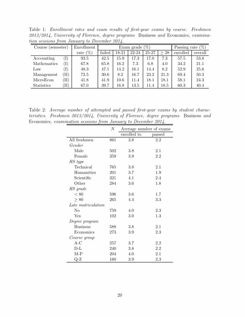
Table 1: Enrollment rates and exam results of first-year exams by course. Freshmen2013/2014, University of Florence, degree programs Business and Economics, examina-tion sessions from January to December 2014.

Course (semester) Enrollment Exam grade (%) Passing rate (%)rate (%) failed 18-21 22-24 25-27 ≥ 28 enrolled overall

Accounting (I) 93.5 42.5 15.9 17.3 17.0 7.3 57.5 53.8Mathematics (I) 67.8 65.8 16.2 7.3 6.8 4.0 34.2 21.1Law (I) 48.3 47.1 14.2 16.1 14.4 8.2 52.9 25.6Management (II) 72.5 30.6 8.2 16.7 23.2 21.3 69.4 50.3MicroEcon (II) 41.8 41.9 10.6 11.4 18.1 18.1 58.1 24.3Statistics (II) 67.0 39.7 16.8 13.5 11.4 18.5 60.3 40.4

Table 2: Average number of attempted and passed first-year exams by student charac-teristics. Freshmen 2013/2014, University of Florence, degree programs Business andEconomics, examination sessions from January to December 2014.

N Average number of examsenrolled to passed

All freshmen 861 3.8 2.2Gender

Male 502 3.8 2.1Female 359 3.9 2.2

HS type

Technical 765 3.8 2.1Humanities 201 3.7 1.9Scientific 321 4.1 2.4Other 284 3.6 1.8

HS grade

< 80 596 3.6 1.7≥ 80 265 4.4 3.3

Late matriculation

No 759 4.0 2.3Yes 102 3.0 1.3

Degree program

Business 588 3.8 2.1Economics 273 3.9 2.3

Course group

A-C 257 3.7 2.2D-L 240 3.8 2.2M-P 204 4.0 2.1Q-Z 160 3.9 2.3

20

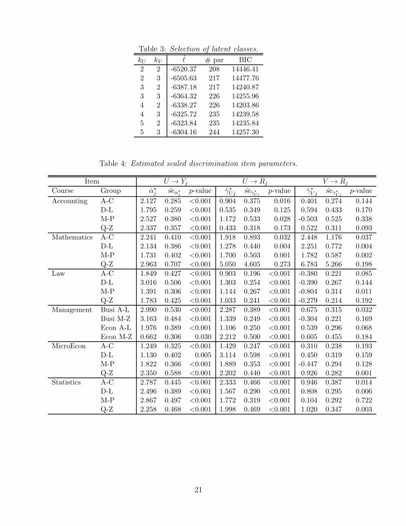
Table 3: Selection of latent classes.

kU kV ℓ # par BIC

2 2 -6520.37 208 14446.412 3 -6505.63 217 14477.763 2 -6387.18 217 14240.873 3 -6364.32 226 14255.964 2 -6338.27 226 14203.864 3 -6325.72 235 14239.585 2 -6323.84 235 14235.845 3 -6304.16 244 14257.30

Table 4: Estimated scaled discrimination item parameters.

Item U → Yj U → Rj V → Rj

Course Group α∗j seα∗

jp-value γ∗Uj seγ∗

Ujp-value γ∗V j seγ∗

V jp-value

Accounting A-C 2.127 0.285 <0.001 0.904 0.375 0.016 0.401 0.274 0.144D-L 1.795 0.259 <0.001 0.535 0.349 0.125 0.594 0.433 0.170M-P 2.527 0.380 <0.001 1.172 0.533 0.028 -0.503 0.525 0.338Q-Z 2.337 0.357 <0.001 0.433 0.318 0.173 0.522 0.311 0.093

Mathematics A-C 2.241 0.410 <0.001 1.918 0.893 0.032 2.448 1.176 0.037D-L 2.134 0.386 <0.001 1.278 0.440 0.004 2.251 0.772 0.004M-P 1.731 0.402 <0.001 1.700 0.503 0.001 1.782 0.587 0.002Q-Z 2.963 0.707 <0.001 5.050 4.605 0.273 6.783 5.266 0.198

Law A-C 1.849 0.427 <0.001 0.903 0.196 <0.001 -0.380 0.221 0.085D-L 3.016 0.506 <0.001 1.303 0.254 <0.001 -0.390 0.267 0.144M-P 1.391 0.306 <0.001 1.144 0.267 <0.001 -0.804 0.314 0.011Q-Z 1.783 0.425 <0.001 1.033 0.241 <0.001 -0.279 0.214 0.192

Management Busi A-L 2.990 0.530 <0.001 2.287 0.389 <0.001 0.675 0.315 0.032Busi M-Z 3.163 0.484 <0.001 1.339 0.249 <0.001 -0.304 0.221 0.169Econ A-L 1.976 0.389 <0.001 1.106 0.250 <0.001 0.539 0.296 0.068Econ M-Z 0.662 0.306 0.030 2.212 0.500 <0.001 0.605 0.455 0.184

MicroEcon A-C 1.249 0.325 <0.001 1.429 0.247 <0.001 0.310 0.238 0.193D-L 1.130 0.402 0.005 3.114 0.598 <0.001 0.450 0.319 0.159M-P 1.822 0.366 <0.001 1.889 0.353 <0.001 -0.447 0.294 0.128Q-Z 2.350 0.588 <0.001 2.202 0.440 <0.001 0.926 0.282 0.001

Statistics A-C 2.787 0.445 <0.001 2.333 0.466 <0.001 0.946 0.387 0.014D-L 2.496 0.389 <0.001 1.567 0.290 <0.001 0.808 0.295 0.006M-P 2.867 0.497 <0.001 1.772 0.319 <0.001 0.104 0.292 0.722Q-Z 2.258 0.468 <0.001 1.998 0.469 <0.001 1.020 0.347 0.003

21

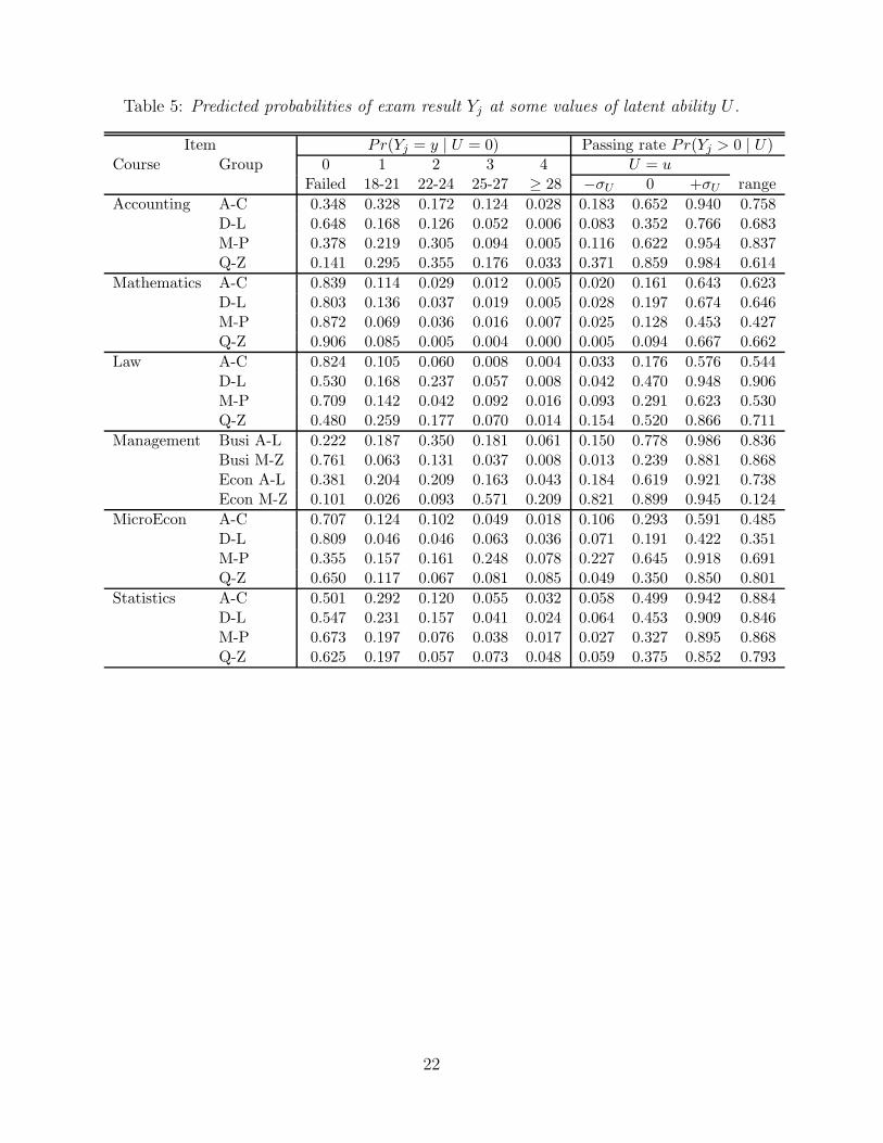
Table 5: Predicted probabilities of exam result Yj at some values of latent ability U .

Item Pr(Yj = y | U = 0) Passing rate Pr(Yj > 0 | U)Course Group 0 1 2 3 4 U = u

Failed 18-21 22-24 25-27 ≥ 28 −σU 0 +σU range

Accounting A-C 0.348 0.328 0.172 0.124 0.028 0.183 0.652 0.940 0.758D-L 0.648 0.168 0.126 0.052 0.006 0.083 0.352 0.766 0.683M-P 0.378 0.219 0.305 0.094 0.005 0.116 0.622 0.954 0.837Q-Z 0.141 0.295 0.355 0.176 0.033 0.371 0.859 0.984 0.614

Mathematics A-C 0.839 0.114 0.029 0.012 0.005 0.020 0.161 0.643 0.623D-L 0.803 0.136 0.037 0.019 0.005 0.028 0.197 0.674 0.646M-P 0.872 0.069 0.036 0.016 0.007 0.025 0.128 0.453 0.427Q-Z 0.906 0.085 0.005 0.004 0.000 0.005 0.094 0.667 0.662

Law A-C 0.824 0.105 0.060 0.008 0.004 0.033 0.176 0.576 0.544D-L 0.530 0.168 0.237 0.057 0.008 0.042 0.470 0.948 0.906M-P 0.709 0.142 0.042 0.092 0.016 0.093 0.291 0.623 0.530Q-Z 0.480 0.259 0.177 0.070 0.014 0.154 0.520 0.866 0.711

Management Busi A-L 0.222 0.187 0.350 0.181 0.061 0.150 0.778 0.986 0.836Busi M-Z 0.761 0.063 0.131 0.037 0.008 0.013 0.239 0.881 0.868Econ A-L 0.381 0.204 0.209 0.163 0.043 0.184 0.619 0.921 0.738Econ M-Z 0.101 0.026 0.093 0.571 0.209 0.821 0.899 0.945 0.124

MicroEcon A-C 0.707 0.124 0.102 0.049 0.018 0.106 0.293 0.591 0.485D-L 0.809 0.046 0.046 0.063 0.036 0.071 0.191 0.422 0.351M-P 0.355 0.157 0.161 0.248 0.078 0.227 0.645 0.918 0.691Q-Z 0.650 0.117 0.067 0.081 0.085 0.049 0.350 0.850 0.801

Statistics A-C 0.501 0.292 0.120 0.055 0.032 0.058 0.499 0.942 0.884D-L 0.547 0.231 0.157 0.041 0.024 0.064 0.453 0.909 0.846M-P 0.673 0.197 0.076 0.038 0.017 0.027 0.327 0.895 0.868Q-Z 0.625 0.197 0.057 0.073 0.048 0.059 0.375 0.852 0.793

22

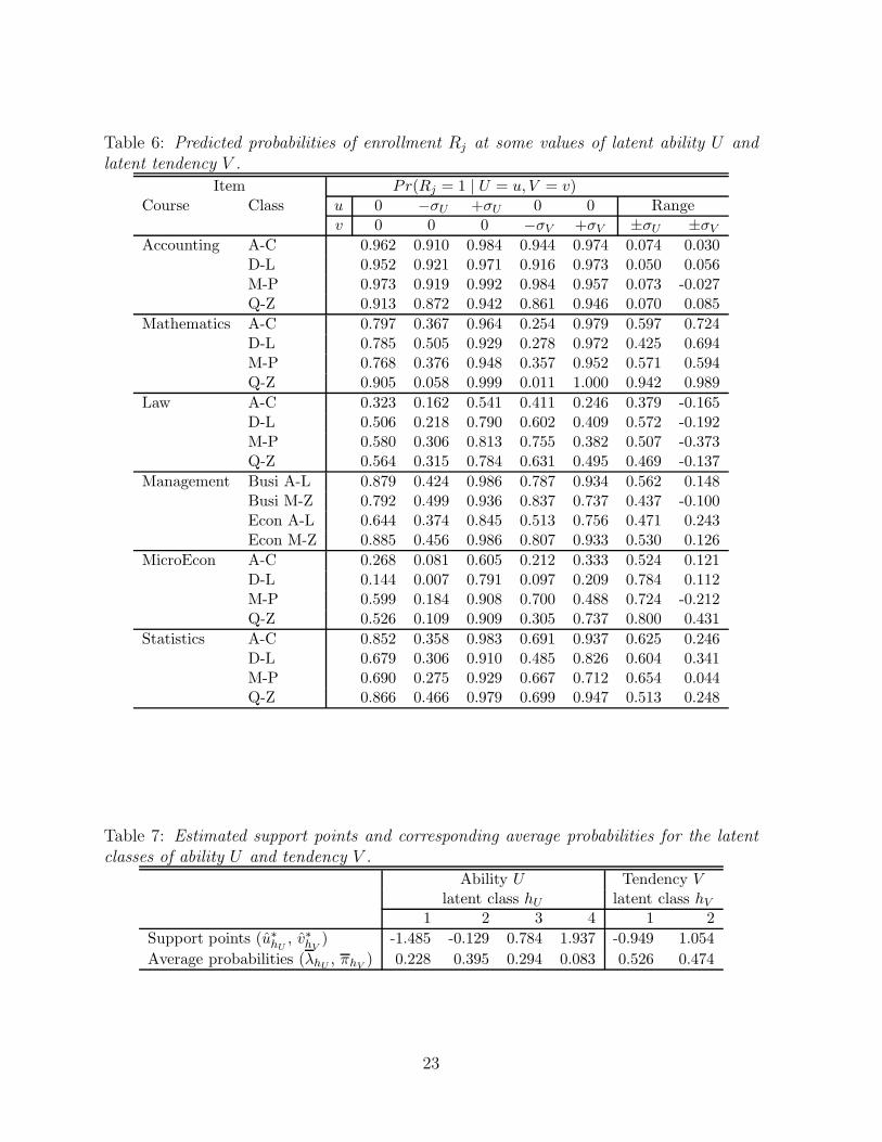
Table 6: Predicted probabilities of enrollment Rj at some values of latent ability U andlatent tendency V .

Item Pr(Rj = 1 | U = u, V = v)Course Class u 0 −σU +σU 0 0 Range

v 0 0 0 −σV +σV ±σU ±σVAccounting A-C 0.962 0.910 0.984 0.944 0.974 0.074 0.030

D-L 0.952 0.921 0.971 0.916 0.973 0.050 0.056M-P 0.973 0.919 0.992 0.984 0.957 0.073 -0.027Q-Z 0.913 0.872 0.942 0.861 0.946 0.070 0.085

Mathematics A-C 0.797 0.367 0.964 0.254 0.979 0.597 0.724D-L 0.785 0.505 0.929 0.278 0.972 0.425 0.694M-P 0.768 0.376 0.948 0.357 0.952 0.571 0.594Q-Z 0.905 0.058 0.999 0.011 1.000 0.942 0.989

Law A-C 0.323 0.162 0.541 0.411 0.246 0.379 -0.165D-L 0.506 0.218 0.790 0.602 0.409 0.572 -0.192M-P 0.580 0.306 0.813 0.755 0.382 0.507 -0.373Q-Z 0.564 0.315 0.784 0.631 0.495 0.469 -0.137

Management Busi A-L 0.879 0.424 0.986 0.787 0.934 0.562 0.148Busi M-Z 0.792 0.499 0.936 0.837 0.737 0.437 -0.100Econ A-L 0.644 0.374 0.845 0.513 0.756 0.471 0.243Econ M-Z 0.885 0.456 0.986 0.807 0.933 0.530 0.126

MicroEcon A-C 0.268 0.081 0.605 0.212 0.333 0.524 0.121D-L 0.144 0.007 0.791 0.097 0.209 0.784 0.112M-P 0.599 0.184 0.908 0.700 0.488 0.724 -0.212Q-Z 0.526 0.109 0.909 0.305 0.737 0.800 0.431

Statistics A-C 0.852 0.358 0.983 0.691 0.937 0.625 0.246D-L 0.679 0.306 0.910 0.485 0.826 0.604 0.341M-P 0.690 0.275 0.929 0.667 0.712 0.654 0.044Q-Z 0.866 0.466 0.979 0.699 0.947 0.513 0.248

Table 7: Estimated support points and corresponding average probabilities for the latentclasses of ability U and tendency V .

Ability U Tendency Vlatent class hU latent class hV

1 2 3 4 1 2

Support points (u∗hU, v∗hV

) -1.485 -0.129 0.784 1.937 -0.949 1.054

Average probabilities (λhU, πhV

) 0.228 0.395 0.294 0.083 0.526 0.474

23

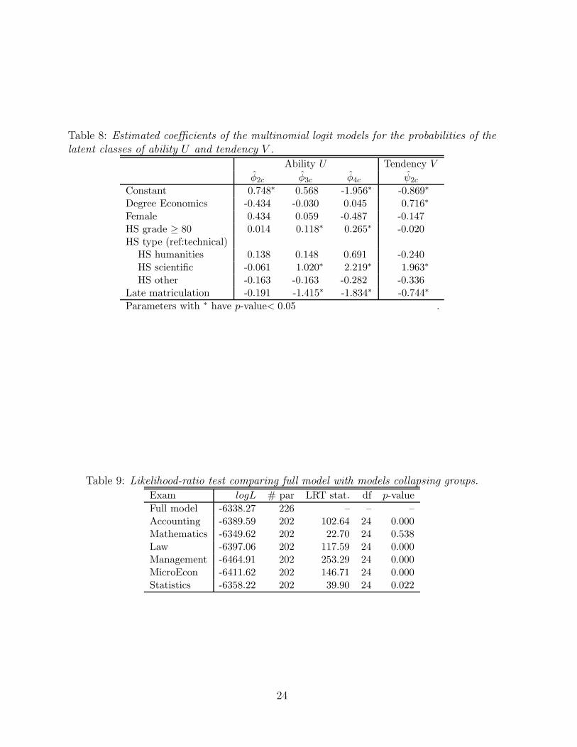
Table 8: Estimated coefficients of the multinomial logit models for the probabilities of thelatent classes of ability U and tendency V .

Ability U Tendency V

φ2c φ3c φ4c ψ2c

Constant 0.748∗ 0.568 -1.956∗ -0.869∗

Degree Economics -0.434 -0.030 0.045 0.716∗

Female 0.434 0.059 -0.487 -0.147HS grade ≥ 80 0.014 0.118∗ 0.265∗ -0.020HS type (ref:technical)

HS humanities 0.138 0.148 0.691 -0.240HS scientific -0.061 1.020∗ 2.219∗ 1.963∗

HS other -0.163 -0.163 -0.282 -0.336Late matriculation -0.191 -1.415∗ -1.834∗ -0.744∗

Parameters with ∗ have p-value< 0.05 .

Table 9: Likelihood-ratio test comparing full model with models collapsing groups.

Exam logL # par LRT stat. df p-value

Full model -6338.27 226 – – –Accounting -6389.59 202 102.64 24 0.000Mathematics -6349.62 202 22.70 24 0.538Law -6397.06 202 117.59 24 0.000Management -6464.91 202 253.29 24 0.000MicroEcon -6411.62 202 146.71 24 0.000Statistics -6358.22 202 39.90 24 0.022

24