Evaluation of Sampling Methods in Constructing Response Surface ...

1

American Institute of Aeronautics and Astronautics

Evaluation of Sampling Methods in Constructing Response

Surface Approximations

L. P. Swiler*, R. Slepoy, A. A. Giunta

Sandia National Laboratories†, Albuquerque, NM 87185-0828 USA

Response surface approximations (RSA) are often used as inexpensive replacements for

computationally expensive computer simulations. Once a RSA has been computed, it is

cheap to evaluate this “meta-model” or surrogate, and thus the RSA is often used in a

variety of contexts, including optimization and uncertainty quantification. Usually, some

method of sampling points over the input domain is used to generate samples of the input

variables. These samples are run through the computer simulation. A response surface

approximation is then generated based on the sample points. This report presents a study

investigating the dependency of the response surface method on the sampling type. The

purpose of this study was to address the question: Does a particular RSA type perform

better (in terms of a better fit) if a particular sampling method is used? The RSA types

examined were kriging, polynomial regression, and multivariate adaptive regression splines

(MARS). The sampling types examined were Latin Hypercube, Halton, Hammersley,

Centroidal Voronoi Tesselation (CVT), and standard Monte Carlo sampling. The example

problems were a 5-dimensional version of Rosenbrock’s function and the Paviani function.

RSA of the three response surface types were developed based on the five sampling methods.

Performance was compared using ANOVA techniques.

* Corresponding Author: US Postal Address: Sandia National Laboratories, P.O. Box 5800, Mail Stop 0370,

Albuquerque, NM 87185-0370, USA; Email: [email protected]; Telephone: 505-844-8093 † Sandia is a multiprogram laboratory operated by Sandia Corporation, a Lockheed Martin Company, for the United

States Department of Energy’s National Nuclear Security Administration under Contract DE-AC04-94AL85000.

This material is declared a work of the U.S. Government and is not subject to copyright protection in the United

States.

2


I. Introduction

Response surface approximations (RSA) are often used as inexpensive replacements for computationally

expensive computer simulations. Once a RSA has been computed, it is cheap to evaluate this “meta-model” or

surrogate, and thus the RSA is often used in a variety of contexts, including optimization and uncertainty

quantification. Usually, some method of sampling points over the input domain is used to generate samples of the

input variables. These samples are run through the computer simulation. A response surface approximation is then

generated based on the sample points. 8

This report presents a study investigating the dependency of the response surface method on the sampling type.

The purpose of this study was to address the question: Does a given RSA type perform better (in terms of a better

fit) if a particular sampling method is used? There is some evidence to suggest that quasi-Monte Carlo methods

perform better than Latin Hypercube when sampling over a small number of input variables17. There is also some

evidence that kriging does not perform well when the points are highly collinear1. Thus, we wanted to investigate

these issues in more detail and provide some guidance within the context of the DAKOTA software framework on

which sampling methods work best for various RSA types.

The RSA types examined were kriging, polynomial regression, and multivariate adaptive regression splines

(MARS). The sampling types examines were Latin Hypercube, Halton, Hammersley, Centroidal Voronoi

Tesselation (CVT), and standard Monte Carlo sampling. The example problems were a 5-dimensional version of

Rosenbrock’s function and a 10-dimension version of Paviani’s function. RSA of the three response surface types

were developed based on the five sampling methods.

II. Sampling Methods

The sampling methods presented in sections 2.1-2.5 below all can be used in uncertainty quantification, where

one wants to understand the effect of input uncertainties on the distribution of outputs. As an example, consider a

variable Y that is a function of other variables X1, X2, …, Xk. This function may be very complicated, for example, a

computer model. A question to be investigated is “How does Y vary when the Xs vary according to some assumed

joint probability distribution?” Related questions are “What is the expected value of Y?” and “What is the 99th

percentile of Y?” The sampling methods can all generate a number of samples of the random variables. It is

convenient to think of the samples as forming an (n × k) matrix of input where the ith row contains specific values of

each of the k input variables to be used on the ith run of the computer model.

A. Latin Hypercube Latin hypercube sampling (LHS) is a stratified sampling method developed to address the need for more

efficient uncertainty assessment. LHS partitions the parameter space into bins of equal probability, with the goal of

attaining a more even distribution of sample points in the parameter space than typically occurs with pure Monte

Carlo sampling.

Latin hypercube sampling, developed by McKay, Conover, and Beckman15, is a constrained sampling method

which selects n different values from each of k variables X1, … Xk in the following manner. The range of each

variable is divided into n non-overlapping intervals on the basis of equal probability. One value from each interval

is selected at random with respect to the probability density in the interval. The n values thus obtained for X1 are

paired in a random manner (equally likely combinations) with the n values of X2. These n pairs are combined in a

random manner with the n values of X3 to form n triplets, and so on, until n k-tuplets are formed. This is the Latin

hypercube sample.

The Latin hypercube sampling technique has been applied to many different computer models over the past

thirty years. A tutorial on Latin hypercube sampling may be found in Iman and Conover12. A recent comparison of

Latin hypercube sampling with other techniques is given in Helton and Davis11. A method for inducing correlations

among the input variables is given in Iman and Conover13. Swiler and Wyss

21 provide a User’s manual for the

current LHS implementation in the DAKOTA software framework.

3


B. Halton Sampling Halton sampling is a type of sampling known as quasi-Monte Carlo sampling. The goal of quasi-Monte Carlo

methods is to produce sequences which have low discrepancy. Discrepancy refers to the nonuniformity of the

sample points within the hypercube. Discrepancy is defined as the difference between the actual number and the

expected number of points one would expect in a particular set B (such as a hyper-rectangle within the unit

hypercube), maximized over all such sets. Low discrepancy sequences tend to cover the unit hypercube reasonably

uniformly. Quasi-Monte Carlo methods produce low discrepancy sequences, especially if one is interested in the

uniformity of projections of the point sets onto lower dimensional faces of the hypercube (usually 1-D: how well do

the marginal distributions approximate a uniform?)

The quasi-Monte Carlo Halton sequence is a deterministic sequence determined by a set of prime bases. The

Halton sequence in base 2 starts with points 0.5, 0.25, 0.75, 0.125, 0.625, etc. The first few points in a Halton base 3

sequence are 0.33333, 0.66667, 0.11111, 0.44444, 0.77777, etc. Notice that the Halton sequence tends to alternate

back and forth, generating a point closer to zero then a point closer to one. An individual sequence is based on a

radix inverse function defined on a prime base. The prime base determines how quickly the [0,1] interval is filled in.

Generally, the lowest primes are recommended.

For more information about the Halton sequence, see References 9, 10, and 14. In cases where a large number

of input variables are sampled, Robinson and Atcitty17 recommend using a leaped sequence, where the user does not

use every term in the Halton sequence but sets a “leap value” to the next prime number larger than the largest prime

base. Using the leaped values in the sequence can help maintain uniformity when generating sample sets for high

dimensions.

C. Hammersley Sampling The Hammersley sequence is the same as the Halton sequence, except the values for the first random variable are

equal to 1/N, where N is the number of samples. Thus, if one wants to generate a sample set of 100 samples for 3

random variables, the first random variable has values 1/100, 2/100, 3/100, etc. and the second and third variables

are generated according to a Halton sequence with bases 2 and 3, respectively. Hammersley sequences can also be

improved but shifting points3. Since we are using a relatively low number of dimensions for this study (five), we

did not use a shifted or leaped version of either the Halton or Hammersley sequences.

D. Centroidal Voronoi Tesselation Centroidal Voronoi Tesselation (CVT) sampling produces a set of sample points that are (approximately) a

Centroidal Voronoi Tessellation. The primary feature of such a set of points is that they have good volumetric

spacing; the points tend to arrange themselves in a pattern of cells that are roughly the same shape. To produce this

set of points, an almost arbitrary set of initial points is chosen, and then an internal set of iterations is carried out.

These iterations repeatedly replace the current set of sample points by an estimate of the centroids of the

corresponding Voronoi subregions. 4

CVT does very well volumetrically: it spaces the points fairly equally throughout the space, so that the points

cover the region and are isotropically distributed with no directional bias in the point placement. There are various

measures of volumetric uniformity which take into account the distances between pairs of points, regularity

measures, etc. Note that CVT does not produce low-discrepancy sequences in lower dimensions, however: the

lower-dimension (such as 1-D) projections of CVT can have high discrepancy. 18

E. Monte Carlo

What we are referring to as “pure” or “plain” Monte Carlo16 involves using a random number generator to

generate random number sequences, with no effort to stratify the samples or construct explicit correlations between

sample values for multiple input dimensions.

F. DAKOTA Implementation This study employs DAKOTA

5 version 3.3 on a 32-bit Intel microprocessor-based computer workstation

running the Fedora Core 3 version of the Red Hat Linux operating system. This version of DAKOTA is available to

the public, under the restrictions of the GNU General Public License, from http://endo.sandia.gov/DAKOTA.

http://endo.sandia.gov/DAKOTA

4


III. Response Surface Approximation Methods

A. Kriging Kriging interpolation techniques were originally developed in the geostatistics and spatial statistics communities

to produce maps of underground geologic deposits based on samples obtained at widely and irregularly spaced

borehole sites2. The basic notion that underpins kriging is that the sample response values exhibit spatial correlation,

with response values modeled via a Gaussian process around each sample location (i.e., samples taken close together

are likely to have highly correlated response values, whereas samples taken far apart are unlikely to have highly

correlated response values). Kriging methods have found wide utility due to their ability to accommodate irregularly

spaced data, their ability to model general surfaces that have many peaks and valleys, and their exact interpolation of

the given sample response values.

The specific form of the kriging model used in this study is described in Giunta and Watson7 and Romero et al.

19

The form of the kriging model is

( ) ( ) 1ˆ ( {1})T

f x r x R fβ β−= + − , (1)

where β is the generalized least squares estimate of the mean response; r(x) is an N x 1 vector of correlations

between the current point x, and all N sample sites in parameter space; R is the N x N correlation matrix of all N

sample sites; f is the vector of N sample site response values; and {1} is an N x 1 vector with all values set to unity.

The terms in the correlation vector and matrix are computed using a Gaussian correlation function. The ith term in

r(x) is given by

2

( )

1exp

n i

i t t ttr x xθ

=

= − − ∑ , (2)

and, similarly, the i,jth term in R is given by

2

( ) ( )

, 1exp

n i j

i j t t ttR x xθ

=

= − − ∑ , (3)

where n is the dimension of the parameter space; t is the index on the dimension of the parameter space; i =

1,…,N; j = 1,…,N; and θ is the n x 1 vector of correlation parameters. In this study, all values of θ are set to unity,

although in general, the values of θ can be estimated from the N sample response values via maximum likelihood

estimation.

However, there are drawbacks to kriging. The form of the kriging model requires the inversion of a potentially

dense N x N matrix, where N is the number of sample points. Thus, the basic kriging method does not scale well for

large N. In addition, if two or more of the sample points are close together, the N x N matrix becomes ill-

conditioned. Thus, while kriging tends to work well for sparse sets of samples, this method tends to break down as

the number of samples increases. Note that the kriging interpolation method is prone to ill-conditioning in the

correlation matrix R as the number of sample points increases. This occurs because of the distance measure that is

computed in Equation (3). As the distance between any two sample points i and j decreases, then the ith and j

th rows

in matrix R become linearly dependent, and in the limit where the points are the same, the matrix R becomes

singular. Thus, this basic kriging method works well for a sparse set of sample points in an n-dimensional parameter

space, but as the number of samples increases (and the inter-point distances decrease), the kriging method becomes

unstable.

B. Polynomial Regression Polynomial regression methods are commonly used to create RSA from a set of data samples. Regression is

popular since the calculations are simple and the resulting function is a closed-form algebraic expression. For

example, a quadratic polynomial has the form:

j

k

i

k

j

ijii

k

i

i XXCXCCXY ∑∑∑= ==

++=1 1

,

1

0)(ˆ (4)

Where )(ˆ XY is the estimate of target function at X and the C0, Ci, Ci,j, are constant coefficients. To calculate

the values of the coefficients, a system of linear equations is formed by applying the above polynomial model at

each of N sampling points. The number of sampling points must be greater than or equal to the number of

5


ascending terms in the polynomial. If equal, then the system of equations is exactly determined and the coefficients

of the saturated polynomial can be immediately solved for and the resulting RSA exactly matches the target values

at all of the sampling points. When more sampling points than terms in the polynomial exist, then the system of

equations is overdetermined, and a regression procedure is invoked to solve for the coefficients. Because the

regression polynomial does not have as many terms as there are data samples to fit, it is over-constrained and cannot

in general match the true Y values at the sample points. Most commonly, the method of least squares is used.

C. Multivariate Adaptive Regression Splines

The multivariate adaptive regression splines (MARS) function approximation method6 is based on a complex,

recursive partitioning algorithm involving truncated power spline basis functions. The form of the MARS model is:

( ) ( ) ( )1 2

1 1

ˆ , ...M M

o m m i m m i j

m m

f x a a B x a B x x= =

= + + +∑ ∑ (5)

where the Bm terms are the basis functions, the am terms are the coefficients of the basis functions, M1 is the

number of one-parameter basis functions, and M2 is the number of two-parameter basis functions. The MARS

software allows the user to select either linear or cubic spline basis functions. Cubic spline basis functions are used

for this study. The regression aspect of the MARS algorithm involves a forward/backward stepping process to

adaptively add/remove spline basis functions from the model. It is this regression process that generates the ao and

am terms in Equation (5). The resulting MARS model is a C2-continuous function of piecewise cubic splines, but it

will not exactly interpolate the data points that were used in calculating the coefficients. Thus, like polynomial

regression, MARS has the ability to create smooth approximations to noisy data. Unlike kriging, MARS appears to

have no upper limit on the number of samples that can be used in the function approximation process.

IV. Results

A. Analysis Approach We used Analysis of Variance (ANOVA) methods to determine if the means of various statistics of interest

(such as root mean square error) were significantly different when using one sampling method vs. another, for a

given response surface type. Analysis of variance is used to examine the correlation between a response variable (in

our case, measures of response surface goodness-of-fit) and the independent variables (in our case, sampling

method). ANOVA extends the two-sample t-test for testing the equality of two population means to a more general

null hypothesis of comparing the equality of more than two means.

We used two goodness-of-fit measures to evaluate the accuracy of a response surface constructed from a

particular set of sample values: root mean squared error (RMSE) and mean absolute error (MAE). The definition of

these terms is given below, where yi = actual or observed value and iy is the value predicted by the response

surface.

∑

∑

=

=

−=

−=

n

i i

ii

i

n

i

i

y

yy

n

yyn

1

2

1

ˆ1MAE

)ˆ(1

RMSE

Note that to evaluate each of these sampling methods, we generated 50 sample sets. Each particular sample set

had 100 sample points in 5 dimensions. We evaluated a 5-dimensional version of the Rosenbrock function at these

100 points. The function is:

∑=

+ −+−=4

1

222

1 ])1()(100[)(i

iii xxxxf

After evaluating the function at the 100 points, we constructed a response surface based on these points, then

used the response surface to predict the values of the Rosenbrock function on a grid. The grid had 9 “levels” of each

6


of the 5 input variables, so the grid had 59049 points. We then constructed error metrics for each of the 50 sample

sets (e.g., each sample set has one value for RMSE and MAE). The ANOVA tests are looking across the 50

samples, to see if the mean RMSE according to LHS sampling (for example) is different from the mean RMSE

according to Halton sampling, etc.

To illustrate the process, each sampling method was used to generate fifty sample sets, each with 100 samples in

5-d. For example, one of the LHS input sets was:

X1 X2 X3 X4 X5 Rosenbrock Fn.

-0.849 1.593 -0.983 -1.417 -0.676 2617.739

-1.752 1.978 -0.293 0.710 0.591 1937.145

0.987 -1.172 -1.301 -0.848 1.945 1986.069

-0.476 -1.833 -1.623 -1.133 1.252 4346.873

-1.522 -0.217 1.781 1.698 0.693 1649.052

-0.425 -1.216 1.296 -1.083 -0.316 1194.997

0.590 0.839 -1.261 -1.732 -0.873 3024.397

0.653 1.712 -1.990 -1.452 0.936 5672.056

1.277 -1.284 0.514 -0.188 -1.565 1262.108

-1.347 -0.844 -0.816 0.461 0.326 957.117 …

Note that the input variables are all bounded between -2 and 2. The predictions were constructed on a 5-d grid

as follows (this example shows a prediction based on a kriging response surface constructed over the input samples):

X1 X2 X3 X4 X5 Rosenbrock Fn. Kriging Prediction

-2.00 1.50 2.00 2.00 1.50 1667.50 1186.91

-1.50 1.50 2.00 2.00 1.50 1096.00 1186.22

-1.00 1.50 2.00 2.00 1.50 1062.50 1185.58

-0.50 1.50 2.00 2.00 1.50 1192.00 1184.99

0.00 1.50 2.00 2.00 1.50 1259.50 1184.46

0.50 1.50 2.00 2.00 1.50 1190.00 1183.99

1.00 1.50 2.00 2.00 1.50 1058.50 1183.58

1.50 1.50 2.00 2.00 1.50 1090.00 1183.22

2.00 1.50 2.00 2.00 1.50 1659.50 1182.92

-2.00 2.00 2.00 2.00 1.50 1837.00 1241.43

-1.50 2.00 2.00 2.00 1.50 1440.50 1241.05

-1.00 2.00 2.00 2.00 1.50 1532.00 1240.69

-0.50 2.00 2.00 2.00 1.50 1736.50 1240.37

0.00 2.00 2.00 2.00 1.50 1829.00 1240.07

-2.00 1.50 2.00 2.00 1.50 1667.50 1186.91

The difference between the actual Rosenbrock function value and the predicted function value was used in to

construct an RMSE and MAE metric for each sample set. Then, we used ANOVA to understand the spread of these

metrics over the 50 sample sets, and to determine if the means were the same. Below we present box plots and

ANOVA results for each response surface type.

7


B. Results for Kriging RSA

cvt=1 lhs=2 halt=3 hamm=4 MC=5

Kriging RMSE

54321

2250

2000

1750

1500

1250

1000

750

500

Boxplot of Kriging RMSE by cvt=1 lhs=2 halt=3 hamm=4 MC=5

Figure 1. Kriging RMSE vs. Sample Type: Rosenbrock Function


Kriging M

AE

54321

0.6

0.5

0.4

0.3

0.2

Boxplot of Kriging MAE by cvt=1 lhs=2 halt=3 hamm=4 MC=5

Figure 2. Kriging MAE vs. Sample Type: Rosenbrock Function

8


Based on the results in Figures 1 and 2, we can see that the mean values of RMSE and MAE are significantly

greater for CVT than for the other sampling methods when using a kriging response surface. For example, more

detailed results for RMSE show that that the mean RMSE for CVT samples is 1251.9, while the mean RMSE for the

other sampling methods is approximately 750. The performance of the other sampling methods was

indistinguishable in terms of comparing the means using a Tukey or Fisher pairwise comparison.

Individual 95% CIs For Mean Based on Pooled StDev

Level N Mean StDev -------+---------+---------+---------+--

1 50 1251.9 260.8 (-*--)

2 50 747.1 88.2 (--*-)

3 50 748.4 77.5 (--*-)

4 50 730.0 77.7 (--*-)

5 50 773.1 109.7 (-*--)

-------+---------+---------+---------+--

800 960 1120 1280

Finally, we looked at the residuals from one “prediction” sample set for each of the sampling methods. This is

shown in Figure 3 below. One can visually see that the residuals from a CVT sample set are higher than those from

the other sample types.

Data

12500100007500500025000-2500

CVT

LHS

Halton

Hammersley

MC

59K Residuals from a Kriging modelbased on various sample types: CVT, LHS, Halton, Hammersley, and MC

Each symbol represents up to 2614 observations.

Figure 3. Kriging Model Residuals from one response surface, evaluated on a grid of 59049 points,

for the 5-D Rosenbrock function.

9


C. Results for Polynomial Regression RSA Figure 4 shows a similar pattern for the various sample types when a polynomial regression response surface is

constructed based on these sample types. We see that the mean value of RMSE is statistically significantly greater

for CVT than for the other sampling methods when using a polynomial regression response surface.


Regression RMSE

54321

1500

1400

1300

1200

1100

1000

900

Boxplot of Regression RMSE by cvt=1 lhs=2 halt=3 hamm=4 MC=5

Figure 4. Polynomial Regression RMSE vs. Sample Type: 5-D Rosenbrock

However, the MAE for CVT is not greater than the other sampling methods when a polynomial regression model

is used, in fact the reverse is true, as shown in Figure 5. The MAE for CVT is the smallest of all the sampling

methods and the mean MAE based on these 50 samples is statistically significantly smaller than the mean MAEs

from the other sampling methods. Also, Hammersley and Halton performed somewhat better than LHS and MC for

MAE:


Level N Mean StDev -+---------+---------+---------+--------

1 50 0.38903 0.00565 (---*---)

2 50 0.43180 0.02692 (---*---)

3 50 0.41749 0.01787 (---*---)

4 50 0.41194 0.01569 (--*---)

5 50 0.43662 0.03466 (---*---)

-+---------+---------+---------+--------

0.384 0.400 0.416 0.432

.

10



Regression M

AE

54321

0.55

0.50

0.45

0.40

Boxplot of Regression MAE by cvt=1 lhs=2 halt=3 hamm=4 MC=5

Figure 5. Polynomial Regression MAE vs. Sample Type: 5-D Rosenbrock

Although the “good” performance of CVT with respect to the mean absolute error metric may seem

contradictory to the “poor” performance of CVT with respect to the root mean squared error metric, one needs to

remember that these metrics track different behavior. The Rosenbrock function is fairly flat in the middle of the

domain chosen for this study, but its value increases sharply at the edges of the domain. All of the response surface

methods did poorly at predicting the 5-D Rosenbrock function at the edges of the domain. Significant errors in

“edge” fitting can lead to large RMSE, while average error is not affected much by lack of fit near the edges

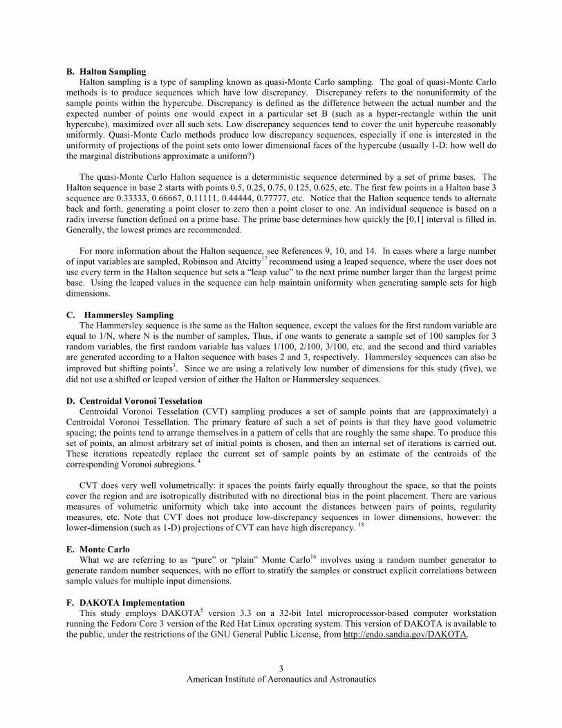
(remember that we are taking average error over 59049 points). Also, it is instructive to look at the placement of

the sample points upon which the regression surface is based. If one looks at a plot of the CVT points in two

dimensions, for example inputs X1 and X2, one can see they are “clustered” as shown in Figure 6. Plotting any of

the other inputs relative to each other (e.g., X3 vs. X5) shows a similar pattern. This clustering may contribute to

the method performing relatively well over all the space but poorly at the edges, which the RMSE metric

emphasizes. Note that there is an approach which “latinizes” or stratifies the CVT samples to give them better 1-D

marginal densities, which may improve their potential use in response surface modeling. This is described in

Reference 18 and is implemented in the DAKOTA software. However, we did not latinize the CVT samples for the

purposes of this study.

11


Placement of X1, X2 in one CVT sample

-2

-1.5

-1

-0.5

0

0.5

1

1.5

2

-2 -1.5 -1 -0.5 0 0.5 1 1.5 2

X1

X2

Figure 6. Placement of X1, X2 in a 100 point CVT sample set

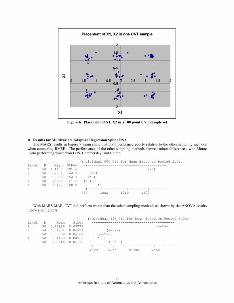
D. Results for Multivariate Adaptive Regression Spline RSA

The MARS results in Figure 7 again show that CVT performed poorly relative to the other sampling methods

when comparing RMSE. The performance of the other sampling methods showed minor differences, with Monte

Carlo performing worse than LHS, Hammersley, and Halton.


Level N Mean StDev -+---------+---------+---------+--------

1 50 1541.7 101.6 (-*)

2 50 826.4 144.7 (*-)

3 50 806.8 154.7 (*-)

4 50 756.8 121.6 (*-)

5 50 891.7 158.9 (-*)

-+---------+---------+---------+--------

750 1000 1250 1500

With MARS MAE, CVT did perform worse than the other sampling methods as shown by the ANOVA results

below and Figure 8:


Level N Mean StDev +---------+---------+---------+---------

1 50 0.46926 0.03771 (--*--)

2 50 0.34834 0.06711 (--*--)

3 50 0.33059 0.06189 (--*--)

4 50 0.31438 0.04752 (--*--)

5 50 0.35646 0.05639 (--*--)

+---------+---------+---------+---------

0.300 0.350 0.400 0.450

12



MARS RMSE

54321

2000

1750

1500

1250

1000

750

500

Boxplot of MARS RMSE by cvt=1 lhs=2 halt=3 hamm=4 MC=5

Figure 7. MARS RMSE vs. Sample Type: 5-D Rosenbrock


MARS M

AE

54321

0.6

0.5

0.4

0.3

0.2

Boxplot of MARS MAE by cvt=1 lhs=2 halt=3 hamm=4 MC=5

Figure 8. MARS MAE vs. Sample Type: 5-D Rosenbrock

13


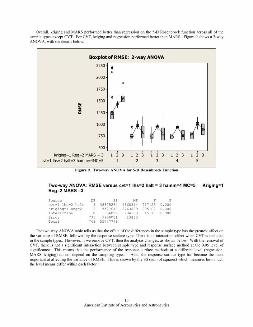
Overall, kriging and MARS performed better than regression on the 5-D Rosenbrock function across all of the

sample types except CVT. For CVT, kriging and regression performed better than MARS. Figure 9 shows a 2-way

ANOVA, with the details below.

RMSE

cvt=1 lhs=2 halt=3 hamm=4MC=5

Kriging=1 Reg=2 MARS = 3

54321

321321321321321

2250

2000

1750

1500

1250

1000

750

500

Boxplot of RMSE: 2-way ANOVA

Figure 9. Two-way ANOVA for 5-D Rosenbrock Function

Two-way ANOVA: RMSE versus cvt=1 lhs=2 halt = 3 hamm=4 MC=5, Kriging=1 Reg=2 MARS =3 Source DF SS MS F P

cvt=1 lhs=2 halt 4 38675254 9668814 717.25 0.000

Kriging=1 Reg=2 2 5527618 2763809 205.02 0.000

Interaction 8 1636826 204603 15.18 0.000

Error 735 9908081 13480

Total 749 55747779

The two-way ANOVA table tells us that the effect of the differences in the sample type has the greatest effect on

the variance of RMSE, followed by the response surface type. There is an interaction effect when CVT is included

in the sample types. However, if we remove CVT, then the analysis changes, as shown below. With the removal of

CVT, there is not a significant interaction between sample type and response surface method at the 0.05 level of

significance. This means that the performance of the response surface methods at a different level (regression,

MARS, kriging) do not depend on the sampling types. Also, the response surface type has become the most

important at affecting the variance of RMSE. This is shown by the SS (sum of squares) which measures how much

the level means differ within each factor.

14


Two-way ANOVA: RMSE versus lhs=2 halt=3 hamm=4 MC=5, Kriging=1 Reg=2 MARS = 3 Source DF SS MS F P

lhs=2 halt=3 ham 3 549074 183025 17.83 0.000

Kriging=1 Reg=2 2 4895728 2447864 238.44 0.000

Interaction 6 122194 20366 1.98 0.066

Error 588 6036389 10266

Total 599 11603386

S = 101.3 R-Sq = 47.98% R-Sq(adj) = 47.00%

Two-way analysis of MAE leads to the same result when CVT is removed: there is no significant interaction

between sampling type and response surface type:

Two-way ANOVA: MAE versus lhs=2 halt=3 hamm=4MC=5, Kriging=1 Reg=2 MARS = 3 Source DF SS MS F P

lhs=2 halt=3 ham 3 0.07291 0.02430 14.93 0.000

Kriging=1 Reg=2 2 3.28768 1.64384 1010.19 0.000

Interaction 6 0.01010 0.00168 1.03 0.402

Error 588 0.95683 0.00163

Total 599 4.32751

S = 0.04034 R-Sq = 77.89% R-Sq(adj) = 77.48%

An important point to note with the 5-D Rosenbrock function is that none of the response surface methods

performed very well with respect to either RMSE or MAE. The values of this function range from 0 to 14436 over

the input domain [-2,2]5. The histogram is shown in Figure 10.

5-D Rosenbrock Function

Frequency

1330011400950076005700380019000

1800

1600

1400

1200

1000

800

600

400

200

0

Histogram of 5-D Rosenbrock Function

Figure 10. Histogram of 5-D Rosenbrock Function

Because the function values vary so widely over a fairly small input domain, these response surface methods are not

very accurate. A root mean square error of 700, for example, or a mean absolute error of 40% which were

demonstrated across sampling methods and response surface approximation types, shows the inaccuracy of these

15


response surfaces. We chose this function to mimic a nonlinear response and to provide an extreme test case. The

next function we chose, the Paviani function, is better behaved in terms of the output not varying widely over the

input domain.

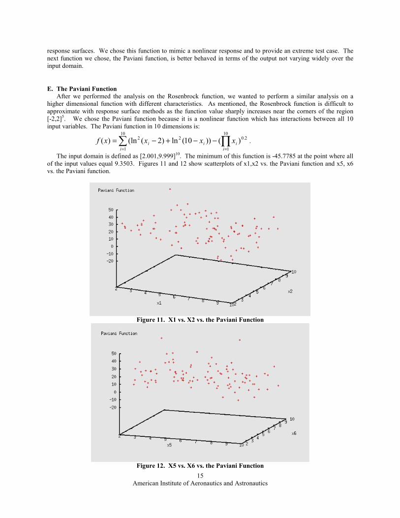
E. The Paviani Function After we performed the analysis on the Rosenbrock function, we wanted to perform a similar analysis on a

higher dimensional function with different characteristics. As mentioned, the Rosenbrock function is difficult to

approximate with response surface methods as the function value sharply increases near the corners of the region

[-2,2]5. We chose the Paviani function because it is a nonlinear function which has interactions between all 10

input variables. The Paviani function in 10 dimensions is:

∑ ∏= =

−−+−=10

1

10

1

2.022 )())10(ln)2((ln)(i i

iii xxxxf .

The input domain is defined as [2.001,9.999]10. The minimum of this function is -45.7785 at the point where all

of the input values equal 9.3503. Figures 11 and 12 show scatterplots of x1,x2 vs. the Paviani function and x5, x6

vs. the Paviani function.

Figure 11. X1 vs. X2 vs. the Paviani Function

Figure 12. X5 vs. X6 vs. the Paviani Function

16


We used a similar procedure as the Rosenbrock function for performing the analysis: We generated 50 sample

sets, where each sample set had 100 samples in the 10-dimensional input space. With each of the 100 samples, we

evaluated the Paviani function, and used those 100 values to construct kriging, regression, and adaptive spline

response surfaces. Then we used the response surfaces to evaluate the function at a grid. The grid was constructed

at three levels for each of the 10 inputs: 3, 5.5, and 8. There were 59049 gridpoints which were used to construct

the metrics such as RMSE and MAE. Note that for the Paviani study, we chose some of the gridpoints to be

slightly on the interior of the domain, whereas for the Rosenbrock function, some of the gridpoints were at the outer

boundaries of the domain.

The results are shown in Sections 4.6-4.8 below. The most striking result is the reversal of CVT. In the

Rosenbrock studies, CVT did not perform well as a sampling method, especially in terms of the RMSE metric. In

the Paviani studies, CVT often outperformed the other sampling methods significantly.

F. Results of Kriging RSA on the Paviani function Figures 13 and 14 below shows the results of the RMSE and the MAE for the kriging RSA of the Paviani

function. The important thing to note is that CVT does not perform well with respect to RMSE, but it performs very

well if the goal is to minimize the mean absolute error of the response surface over the grid. The CVT results are

statistically significantly different than the rest of the sampling methods both for RMSE and for MAE.


Kriging RMSE

54321

16

14

12

10

8

6

4

2

Boxplot of Kriging RMSE by cvt=1 lhs=2 halt=3 hamm=4 MC=5

Figure 13. Kriging RMSE vs. Sample Type: Paviani function

17



Kriging M

AE

54321

5

4

3

2

1

0

Boxplot of Kriging MAE by cvt=1 lhs=2 halt=3 hamm=4 MC=5

Figure 14. Kriging MAE vs. Sample Type: Paviani function

G. Results of Polynomial Regression RSA on the Paviani function Figure 15 shows the results of the RMSE for the kriging RSA of the Paviani function. The Hammersley function

performed horribly, with several values of RMSE on the order of 109.


Reg RMSE

54321

1.8000E+10

1.6000E+10

1.4000E+10

1.2000E+10

1.0000E+10

8000000000

6000000000

4000000000

2000000000

0

Boxplot of Reg RMSE by cvt=1 lhs=2 halt=3 hamm=4 MC=5

Figure 15. Polynomial Regression RMSE vs. Sample Type: Paviani function

18


The likely reason for this is that all 10 variables are important in the Paviani function. In Hammersley sampling,

the first variable is sampled according to a 1/N scheme, where N is the number of samples. For example, if you are

sampling 2 random variables between 0 and 1, with 100 samples, the first variable would have values of 1/100,

2/100, etc. This method of sampling causes the matrix (X’X) to become nearly singular, where X is the matrix of

sample values. Since one needs to invert the (X’X) matrix to obtain the regression coefficients, we see numerical

problems when the condition number of this matrix is very high, for example, around 30. In addition, both

Hammersley and Halton sampling can lead to highly correlated values between input variables. For example, the

correlation between input dimensions X1 and X2 looks very good as shown in Figure 16, but the correlation

between X1 and X4 shows high correlation as shown in Figure 17:

Placement of X1 vs. X2 in one Hammersley

Sample

-2

-1.5

-1

-0.5

0

0.5

1

1.5

2

-2 -1 0 1 2

X1

X2

Figure 16. One 100-point sample set showing X1 vs. X2 in a Hammersley Sample

Placement of X1 vs. X4 in one Hammersley

Sample

-2

-1.5

-1

-0.5

0

0.5

1

1.5

2

-2 -1 0 1 2

X1

X2

Figure 17. One 100-point sample set showing X1 vs. X4 in a Hammersley Sample

19


We were aware of the possibility of the correlations3,17

but we expected it to happen for much larger prime bases

than the ones being used to generate these 5-d or 10-d input sets. To avoid correlations amongst inputs in both

Halton and Hammersley sequences, it is possible to implement a “fix” which involves skipping values of the

sequence when generating data. This is implemented in DAKOTA and is described in the DAKOTA reference

manual, however we did not use it in this study.

For the purposes of comparing the other sampling methods, we left the Hammersley sampling out and performed

the ANOVA on the regression surfaces for the Paviani function. One can see that CVT does very well with respect

to both the RMSE and MAE metrics as shown in Figures 18 and 19.

cvt=1 lhs=2 halton=3 MC=5

Reg RMSE less Hamm

5321

30

25

20

15

10

5

0

Boxplot of Reg RMSE less Hamm by cvt=1 lhs=2 halton=3 MC=5

Figure 18. Polynomial Regression RMSE vs. Sample Type omitting Hammersley: Paviani function

cvt=1 lhs=2 halton=3 MC=5

Reg M

AE less Hamm

5321

8

7

6

5

4

3

2

1

0

Boxplot of Reg MAE less Hamm by cvt=1 lhs=2 halton=3 MC=5

Figure 19. Polynomial Regression MAE vs. Sample Type omitting Hammersley: Paviani function

20


H. Results of Multivariate Adaptive Regression Spline (MARS) RSA on the Paviani function

Figures 20 and 21 show the results of the RMSE and the MAE for the MARS RSA of the Paviani function.

MARS performed very well on this function.


MARS RMSE

54321

14

12

10

8

6

4

2

Boxplot of MARS RMSE by cvt=1 lhs=2 halt=3 hamm=4 MC=5

Figure 20. MARS RMSE vs. Sample Type : Paviani function


MARS M

AE

54321

3.5

3.0

2.5

2.0

1.5

1.0

Boxplot of MARS MAE by cvt=1 lhs=2 halt=3 hamm=4 MC=5

Figure 21. MARS MAE vs. Sample Type : Paviani function

The two-way ANOVA results are shown in Figure 22 for RMSE. Note that we removed Hammersley sampling

from this analysis because of the very ill-fitting in the regression case. In general, MARS and kriging were better

21


response surface approximations than polynomial regression because the Paviani function varies highly in a local

region, and the local fitting techniques tend to work better than global methods. CVT again produces a different

type of interaction than the other sampling methods. It is interesting to note that regression performs better with

CVT than the kriging or MARS.

RMSE

cvt=1 lhs=2 halt=3 MC=5


5321

321321321321

30

25

20

15

10

5

0

Boxplot of RMSE on Paviani function

Figure 22. Two-way ANOVA for Paviani Function RMSE

Two-way ANOVA: RMSE versus cvt=1 lhs=2 halt=3 MC=5, Krig=1 Reg=2 MARS = 3 Source DF SS MS F P

cvt=1 lhs=2 halt 3 1115.66 371.887 77.47 0.000

Kriging=1 Reg=2 2 470.48 235.242 49.00 0.000

Interaction 6 2653.71 442.285 92.13 0.000

Error 588 2822.78 4.801

Total 599 7062.64

cvt=1

lhs=2 Individual 95% CIs For Mean Based on

halt=3 Pooled StDev

MC=5 Mean -+---------+---------+---------+--------

1 5.00638 (--*--)

2 7.55194 (--*--)

3 8.77014 (--*--)

5 7.39510 (--*--)

-+---------+---------+---------+--------

4.8 6.0 7.2 8.4

Kriging=1 Individual 95% CIs For Mean Based on

Reg=2 Pooled StDev

MARS = 3 Mean +---------+---------+---------+---------

1 7.71176 (---*----)

2 7.89772 (----*---)

3 5.93319 (----*---)

+---------+---------+---------+---------

5.60 6.30 7.00 7.70

22


When we look at the performance of the sampling methods and response surface types on minimizing MAE, we

see different behavior, as shown in Figure 23. In this figure, regression and MARS tended to perform better than

kriging in producing lower mean absolute error metrics.

MAE

cvt=1 lhs=2 halt=3 MC=5


5321

321321321321

8

7

6

5

4

3

2

1

0

Boxplot of MAE on Paviani Function

Figure 23. Two-way ANOVA for Paviani Function MAE

Two-way ANOVA: MAE versus cvt=1 lhs=2 halt=3 MC=5, Krig=1 Reg=2 MARS = 3 Source DF SS MS F P

cvt=1 lhs=2 halt 3 315.789 105.263 277.64 0.000

Kriging=1 Reg=2 2 142.149 71.074 187.47 0.000

Interaction 6 43.601 7.267 19.17 0.000

Error 588 222.929 0.379

Total 599 724.469

cvt=1

lhs=2 Individual 95% CIs For Mean Based on

halt=3 Pooled StDev

MC=5 Mean ------+---------+---------+---------+---

1 0.93474 (-*)

2 2.20777 (-*)

3 2.93707 (-*-)

5 2.28814 (-*-)

------+---------+---------+---------+---

1.20 1.80 2.40 3.00

Kriging=1 Individual 95% CIs For Mean Based on

Reg=2 Pooled StDev

MARS = 3 Mean ----+---------+---------+---------+-----

1 2.77839 (-*--)

2 1.79290 (-*--)

3 1.70451 (--*-)

----+---------+---------+---------+-----

1.75 2.10 2.45 2.80

23


The overall trends are that CVT does best and Halton worst for both MAE and RMSE on the Paviani function.

Kriging produced significantly higher (worse) MAE metrics than the MARS or regression, and MARS did much

better at producing good RMSE metrics than regression or kriging. Note that for both RMSE and MAE with the

Paviani function, there are some interaction effects between the sampling type and response surface type. The

interaction was most significant with CVT, since the CVT results per response surface type had different trends than

the other sampling types.

V. Summary

Many studies have been done examining the efficacy of sampling methods with respect to various metrics such

as uniformity and point placement. However, we have not found many studies which look at the sampling methods

and how they perform with various response surface methods. This study has attempted to do that. We examined

two problems with 5 input variables (the 5-D version of the Rosenbrock function) and 10 input variables (the

Paviani function) respectively. While these may not seem like high dimensional problems, many of the studies in

the literature only use 2 or 3 input variables. This work extends our understanding to larger problems. Note that we

did not include sample size as a factor under analysis. We fixed the sample size at 100, based on what we have seen

done in real applications with approximately the same number of input variables. We did perform extensive tests, in

that we generated 50 replicates of the 100 size sample for each sample type, and used those replicates to generate

kriging, regression, and MARS response surfaces. The response surface accuracy was then evaluated over a grid

with 59049 points to calculate RMSE and MAE, and ANOVA studies were used to look at mean differences in

factor levels.

We had hoped to find some clear trends or interactions between sample type and response surface method. We

did not. We did see some interesting behavior. CVT produced some unusual results. It was the worst performing

sampling method on the Rosenbrock function in terms of RMSE and MAE, but it was the best sampling method on

the Paviani function. We feel that CVT warrants further investigation. When we removed CVT from the analysis

of the Rosenbrock function, the performance of the other sampling methods (LHS, Halton, Hammersley, and MC)

was indistinguishable. This is an important result, saying that the sample type essentially doesn’t matter, at least for

the Rosenbrock function. Overall, MARS and kriging appeared to produce the best overall fits to the 5-D

Rosenbrock function.

With the Paviani function, we found that CVT performed significantly better than the other sampling methods in

terms of RMSE and MAE. Halton sampling did not perform well. Hammersley sampling also did not perform

well, especially when used with polynomial regression surface approximations. Regression was not able to produce

reasonable response surface models with Hammersley samples because of the correlations in inputs. This

emphasizes that one needs to be cautious in the choice of sampling method used with response surface type. In the

Paviani results, MARS did very well at producing low RMSE and MAE. However, regression did well only on one

metric: regression did well minimizing MAE but not RMSE. Kriging did not do particularly well on either. This

demonstrates the fact that different response surface approximations have characteristics that will produce different

results depending on one’s metric of interest: overall scaled accuracy as measured by a mean absolute error,

extreme errors which are emphasized in RMSE, overall min or max error, etc.

We did compare our results with those of Simpson, Lin, and Chen20. They also did a comparison of sampling

methods and response surface type on two problems, one with 3 input variables and one with 14 input variables.

Both problems exhibited nonlinear behavior. Simpson et al. showed some general trends in their paper. For

example, the Hammersley sequence gave low results for RMSE, but often was quite high when measuring

maximum absolute deviation. Overall, they found that orthogonal arrays and quasi-uniform designs tended to do

better than pure random or Latin Hypercube designs. We did not find that in our study. They did mention that

Hammersley sampling was not able to be used with regression modeling on their 14 variable problem because of the

singular matrix (X’X), which agrees with our results. Finally, many of their results had a similar interpretation as

ours: certain response surface types worked well on one function but not another, certain sampling types worked

well with respect to RMSE but not MAE or vice-versa, etc. Based on our study and Simpson, Lin, and Chen’s

study, we feel there is no “silver bullet” approach. When using sampling methods to construct response surface

approximations, the analyst must be aware of various pitfalls, and ideally use at least two types of sampling and

24


response surface approximations to understand the characteristics of his or her problem to model it reasonably

accurately with a response surface model.

VI. References

1. Booker, Andrew. “Well-conditioned Kriging Models for Optimization of Computer Simulations.” Technical Document

Series, M&CT-TECH-002, Phantom Works, Mathematics and Computing Technology, The Boeing Company, Seattle, WA,

2000.

2. Cressie, N. (1991), Statistics of Spatial Data, John Wiley and Sons, New York, NY.

3. Diwekar U. M. and J. R. Kalagnanam (1997). "An Efficient Sampling Technique for

Optimization Under Uncertainty", AIChE Journal, 43, 440.

4. Du, Q., V. Faber, and M. Gunzburger,1999. "Centroidal Voronoi Tessellations: Applications and Algorithms," SIAM

Review, Volume 41, 1999, pages 637-676.

5. Eldred, M.S., Giunta, A.A., van Bloemen Waanders, B.G., Wojtkiewicz, S.F., Jr., Hart, W.E. and Alleva, M.P. (2001),

DAKOTA Users Manual: Version 3.1, Sandia Technical Report SAND2001-3796, Sandia National Laboratories, Albuquerque,

NM. (see: http://endo.sandia.gov/DAKOTA/software.html)

6. Friedman, J.H. (1991), ‘‘Multivariate Adaptive Regression Splines,’’ Annals of Statistics, Vol. 19, No. 1, pp. 1-141.

7. Giunta, A. A., and Watson, L. T., “A Comparison of Approximation Modeling Techniques: Polynomial Versus

Interpolating Models,” AIAA Paper 98-4758 in Proceedings of the 7th AIAA/USAF/NASA/ISSMO Symposium on

Multidisciplinary Analysis and Optimization, St. Louis, MO, Sept. 1998, pp. 392-404.

8. Giunta, A. A., Wojtkiewicz, S. F., Jr., and Eldred, M. S. (2003), ''Overview of Modern Design of Experiments Methods for

Computational Simulations,'' paper AIAA-2003-0649 in Proceedings of the 41st AIAA Aerospace Sciences Meeting and Exhibit,

Reno, NV.

9. Halton, J. H. "On the efficiency of certain quasi-random sequences of points in evaluating multi-dimensional integrals,

Numerische Mathematik,Volume 2 pages 84-90.

10. Halton, J. H. and G. B. Smith, 1964. Algorithm 247: Radical-Inverse Quasi-Random Point Sequence, Communications

of the ACM, Volume 7, pages 701-702.

11. Helton, J. C. and Davis, F. J. (2001). “Latin Hypercube Sampling and the Propagation of Uncertainty in Analyses of

Complex Systems.” Technical Report SAND2001-0417, Sandia National Laboratories, Albuquerque, NM.

12. Iman, R.L., and Conover, W.J. (1982a). “Sensitivity Analysis Techniques: Self-Teaching Curriculum,” Nuclear

Regulatory Commission Report, NUREG/CR-2350, Technical Report SAND81-1978, Sandia National Laboratories,

Albuquerque, NM.

13. Iman, R.L., and Conover, W.J. (1982b). “A Distribution-Free Approach to Inducing Rank Correlation Among Input

Variables,” Communications in Statistics, B11(3), 311-334.

14. Kocis, L. and W. Whiten, 1997. "Computational Investigations of Low-Discrepancy Sequences," ACM Transactions on

Mathematical Software, Volume 23, Number 2, 1997, pages 266-294.

15. McKay, M.D., Beckman, R.J., and Conover, W.J. (1979), “A Comparison of Three Methods for Selecting Values of

Input Variables in the Analysis of Output from a Computer Code,” Technometrics, Vol. 21, No. 2, pp. 239-245.

16. Metropolis N. and Ulam, S., “The Monte Carlo Method,” Journal of the American Statistical Association, Vol. 44, No.

247, 1949, pp. 335-341.

17. Robinson, D.G. and C. Atcitty, 1999. "Comparison of Quasi- and Pseudo-Monte Carlo Sampling for Reliability and

Uncertainty Analysis." Proceedings of the AIAA Probabilistic Methods Conference, St. Louis MO, AIAA99-1589.

18. Romero, V.J., Burkardt, J.V., Gunzburger, M.D., and J.S. Peterson (2003). “Initial Evaluation of Pure and “Latinized”

Centroidal Voronoi Tesselation for Non-Uniform Statistical Sampling.” SAMO Conference Paper, 2003.

19. Romero, V. J., Swiler, L. P., and Giunta, A. A., ''Construction of Response Surfaces Based on Progressive-Lattice-

Sampling Experimental,'' Structural Safety, Vol. 26, No. 2, 2004, pp. 201-219.

20. Simpson, T., Dennis, L., and Chen, W. (2002). “Sampling Strategies for Computer Experiments: Design and Analysis”

Journal of International Journal of Reliability and Application, 2(3), 209-240.

21. Swiler, L. P. and Wyss, G. D., “A User’s Guide to Sandia’s Latin Hypercube Sampling Software: LHS UNIX

Library/Standalone Version,” Sandia Technical Report SAND2004-2439, Sandia National Laboratories, Albuquerque, NM,

2004.

Evaluation of Sampling Methods in Constructing Response Surface ...

Documents

Transcript of Evaluation of Sampling Methods in Constructing Response Surface ...