ORIGINAL PAPER

Evaluation of Rock Slope Stability Conditions ThroughDiscriminant Analysis

Allan Erlikhman Medeiros Santos . Milene Sabino Lana . Ivo Eyer Cabral .

Tiago Martins Pereira . Masoud Zare Naghadehi . Denise de Fatima Santos da Silva .

Tatiana Barreto dos Santos

Received: 23 October 2017 /Accepted: 26 July 2018

� Springer Nature Switzerland AG 2018

Abstract A methodology to predict the stability

status of mine rock slopes is proposed. Two techniques

of multivariate statistics are used: principal compo-

nent analysis and discriminant analysis. Firstly, prin-

cipal component analysis was applied in order to

change the original qualitative variables into quanti-

tative ones, as well as to reduce data dimensionality.

Then, a boosting procedure was used to optimize the

resulting function by the application of discriminant

analysis in the principal components. In this research

two analyses were performed. In the first analysis two

conditions of slope stability were considered:

stable and unstable. In the second analysis three

conditions of slope stability were considered: stable,

overall failure and failure in set of benches. A

comprehensive geotechnical database consisting of

18 variables measured in 84 pit-walls all over the

world was used to validate the methodology. The

discriminant function was validated by two different

procedures, internal and external validations. Internal

A. E. M. Santos � M. S. Lana (&) �I. E. Cabral � T. B. dos SantosGraduate Program in Mineral Engineering – PPGEM,

Federal University of Ouro Preto – UFOP, Campi Morro

do Cruzeiro, Bauxita, Ouro Preto,

Minas Gerais CEP: 35400000, Brazil

e-mail: milene@ufop.edu.br

A. E. M. Santos

e-mail: allanboni@hotmail.com

I. E. Cabral

e-mail: cabralmg@oul.com.br

T. B. dos Santos

e-mail: tati.barreto12@gmail.com

T. M. Pereira

Department of Statistics, Federal University of Ouro Preto

– UFOP, Campi Morro do Cruzeiro, Bauxita, Ouro Preto,

Minas Gerais CEP: 35400000, Brazil

e-mail: tiago.martin@gmail.com

M. Zare Naghadehi

Department of Mining Engineering, Hamedan University

of Technology, Hamedan, Iran

e-mail: masoud.zare@hotmail.com

D. de Fatima Santos da Silva

Graduate Geotechnical Center School of Mines,

Geotechnical Nucleus, Federal University of Ouro Preto –

UFOP, Campi Morro do Cruzeiro, Bauxita, Ouro Preto,

Minas Gerais CEP: 35400000, Brazil

e-mail: denisefss@yahoo.com.br

123

Geotech Geol Eng

https://doi.org/10.1007/s10706-018-0649-x(0123456789().,-volV)(0123456789().,-volV)

validation presented an overall probability of success

of 94.73% in the first analysis and 68.42% in the

second analysis. In the second analysis the main

source of errors was due to failure in set of benches. In

external validation, the discriminant function was able

to classify all slopes correctly, in analysis with two

conditions of slope stability. In the external validation

in the analysis with three conditions of slope stability,

the discriminant function was able to classify six

slopes correctly of a total of nine slopes. The proposed

methodology provides a powerful tool for rock slope

hazard assessment in open-pit mines.

Keywords Multivariate statistics � Rock slope

stability � Principal component analysis � Boostingtechnique � Discriminant analysis

1 Introduction

Slope failures are recurring in many situations, leading

to serious hazards and consequences. Landslides in

urban environments, for instance, can be of great

proportions, affecting large inhabited areas. In road

cuts slope failures can cause accidents and traffic

disruption. In open-pit mines steeper slopes are highly

desired on account of their positive economic impact

on cash flow of large projects. Steeper slope angles,

however, result in an increased risk of failure.

Traditionally, the slope failure evaluation is assessed

by stability analyses such as limit equilibriummethods

and 2D/3D numerical modelling (see e.g. Wyllie and

Mah 2004; Read and Stacey 2009). Among the limit

equilibrium methods there are deterministic and

probabilistic approaches. Probabilistic methods are

based on a quantitative analysis of the probability of

failure, considering many different scenarios of

strength parameters and loading conditions. Deter-

ministic methods are based on the safety factor

calculation of a slope in an established scenario of

unchanged strength parameters and loading condi-

tions. In many situations the discrimination of the

slopes according to their stability condition might help

to find out those slopes which can present serious

hazards. When many slopes must be evaluated tech-

niques of multivariate statistics are powerful tools to

detect hazardous situations which require proper and

detailed stability analyses.

Multivariate statistics have been used in the liter-

ature for different purposes as well as the boosting

procedure. The boosting technique has been imple-

mented in algorithms in order to optimize functions

such as in Lin (2011) and Wu et al. (2015). Another

example is the research developed by Massumi and

Gholami (2016). They use principal component anal-

ysis for investigation of structural damage caused by

seismic events. Multivariate statistical methods have

also been applied in geology and in engineering

geology for a variety of problems. A typical problem

extensively studied is landslide susceptibility map-

ping. Multiple regression models, such as logistic

regression, were used to improve susceptibility map-

ping accuracy. Researches with this focus were

presented by Yilmaz (2009), Erener et al. (2017) and

Ahmed and Dewan (2017). In mining, discriminant

analysis was also used to develop a criterion for

stability of underground excavations (Nickson 1992).

Another interesting application of multivariate

analysis in mining industry was presented by Kulati-

lake et al. (2012). These authors used multivariate

models to predict mean particle size in rock blast

fragmentation. A cluster analysis was done to separate

a database composed of 97 blasting data into two

groups based on rock stiffness, which were confirmed

by the application of discriminant analysis. Finally a

neural network model was applied to predict mean

particle size resulting from blasting fragmentation.

In problems involving rock slope failures, there has

been few applications in the literature. This research

proposes a methodology for the assessment of the rock

slope stability status condition based on the applica-

tion of multivariate statistical techniques. The multi-

variate statistical techniques used in this research are

the principal component analysis (PCA) and the

boosting analysis through Fisher’s linear discriminant

analysis.

The methodology was applied in the database built

and organized by Zare Naghadehi et al. (2013). The

geotechnical database presents eighteen parameters,

which are ratings, related to geomechanical parame-

ters surveyed at open pit mines around the world.

Besides the 18 variables, the stability condition of the

slopes (stable or unstable) is known. Zare Naghadehi

et al. (2013) used this database to propose an

instability index for open-pit mine slopes, defined in

their research as Mine Slope Instability Index (MSII).

The authors proposed the use of these eighteen

123

Geotech Geol Eng

parameters, based on the fact that they can be easily

obtained at the field and they are important parameters

related to rock slope stability.

The model proposed in this research can be used to

know the slope stability condition of an untested slope.

The model is also capable of predicting the most

hazardous situations in a group of rock slopes.

2 Theoretical Basis

2.1 Principal Component Analysis

The principal component analysis technique (PCA)

was proposed by Pearson (1901) and developed later

by Hottelling (1933). Principal components can

replace the original variables, besides reducing the

number of variables of the model.

In principal component analysis technique the

principal axes of the multi-dimensional configuration

of the studied data are determined as well as the

coordinates of each sample on these new axes.

Therefore, the principal component analysis technique

consists of a rotation of the original coordinate axes in

the direction of the principal axes. The new variables

(principal components) are linear combinations of the

p original variables of the data set. If the database has

p variables, the PCA can change the system into

k components, where k B p.

The principal components are given by Eq. (1).

Yj ¼ ej1X1 þ ej2X2 þ . . .þ ejpXp ð1Þ

where X1;X2; . . .;Xp are the original variables;

eij are the eigenvectors of the covariance or

correlation matrix of the original data.

The database represented by the matrix X is

constituted by n rows of individuals and p columns

of variables. Table 1 shows the matrix X where n are

the samples and p are the variables.

In this research the correlation matrix was used.

The number of principal components was defined

using the criterion proposed by Kaiser (1958). The

Kaiser’s criterion uses the eigenvalues greater than

one, i.e., it keeps the linear combinations that explain

at least the amount of variance of an original standard

variable, see Johnson and Wichern (1998). This

criterion can be envisaged in the scree plot showed

in Fig. 1. Another way to select the number of the

principal components also uses the scree plot, as

proposed by Cattell (1966). In this graph, it is possible

to see from which principal component the eigenval-

ues are stabilized, meaning that from this point, the

eigenvalues approach zero.

This research used the principal component anal-

ysis not only to reduce database dimensions, but also

to change original qualitative variables into new

quantitative ones (the scores).

2.2 Discriminant Analysis

The discriminant analysis is a technique used for

classifying the elements of a sample in different

populations. The classification rule is built using a

function able to distinguish between two or more

groups through original features that must be known

for all the groups. Fisher (1936) presented a solution

for the problem based on a linear combination of these

original features.

Fisher’s discriminant function is given by Eq. (2).

D Xð Þ ¼ L0 � X ¼ l1 � l2½ �0X�1�X ð2Þ

where D Xð Þ is the discriminant function; L0 is the

discriminant vector; X is the random vector X

containing the variables of the populations; l01 is the

multivariate average vector of the population 1; l02 isthe multivariate average vector of the population 2;

P

is the population common covariance matrix.

The Eq. (3) shows the value of the discriminant

function for a particular observation xo.

D x0ð Þ ¼ l1 � l2½ �0X�1�x0 ð3Þ

The classification rules based on the Fisher’s

discriminant function for the case of two populations

are given by Eqs. (4) and (5).

Table 1 Matrix X of original variables

Sample Variables

X1 X2 … Xp

1 x11 x12 … x1p

: : : : :

N xn1 xn2 … xnp

123

Geotech Geol Eng

D x0ð Þ ¼ l1 � l2½ �0X�1�x0�

1

2D l1ð Þ þ D l2ð Þ½ �; to

x0 ! p1

ð4Þ

D x0ð Þ ¼ l1 � l2½ �0X�1�x0\

1

2D l1ð Þ þ D l2ð Þ½ �; to

x0 ! p2

ð5Þ

A common covariance matrixP

can be estimated

through the estimation of the covariance matrix of the

populations p1 and p2. The common covariance matrixPis calculated through Eq. (6), according to Ander-

son (1984), replacingP

by the known covariance

matrix of the samples S. This equation can only be

used when there is homocedasticity between the

populations p1 and p2.

Sc ¼n1 � 1

n1 � 1ð Þ þ n2 � 1ð Þ

� �� S1

þ n2 � 1

n1 � 1ð Þ þ n2 � 1ð Þ

� �� S2 ð6Þ

where Sc is the sample common covariance matrix; n1is the number of observations in p1; n2 is the number of

observations in p2; S1 is the covariance matrix of p1; S2is the covariance matrix of p2.

As l1, l2 are also unknown the Fisher’s discrim-

inant function is obtained replacing them by the

respective sample quantities, as shown in the Eq. (7).

D xð Þ ¼ L0 � x ¼ x1 � x2½ �0S�1c � x ð7Þ

where D xð Þ is the Fisher’s discriminant function; L0 isthe estimated discriminant vector; x is the random

vector containing the variables of the samples; x1 is the

multivariate average vector of the sample 1; x2 is the

multivariate average vector of the sample 2; Sc is the

common covariance matrix.

Johnson and Wichern (1998) explained that there

are two types of errors in the classification of two

populations. The error 1 is defined when the sample

element belongs to the population 1 but the classifi-

cation rule allocates it in the population 2. The error 2

is defined when the sample element belongs to the

population 2 but the classification rule allocates it in

the population 1. The Eqs. (8) and (9) show the

probability of these two types of errors.

Prob Error1ð Þ ¼ p 2j1ð Þ ð8Þ

Prob Error2ð Þ ¼ p 1j2ð Þ ð9Þ

The overall probability of success (OPS) is shown

in Eq. (10). The apparent error rate (AER) is show in

Eq. (11).

OPS ¼ n11 þ n22

n1 þ n2ð10Þ

AER ¼ 1:0� OPS ð11Þ

where n11 is the number of sample elements of the

population 1 which were correctly allocated in pop-

ulation 1; n22 is the number of sample elements of the

population 2 which were correctly allocated in pop-

ulation 2; n1 is the number of samples of the

population 1; n2 is the number of samples of the

population 2.

This research used the discriminant analysis to

obtain a classifier that is the starting classifier of the

boosting procedure. This technique is referred as the

boosting algorithm via discriminant analysis. The

boosting procedure improves this classifier, expanding

its discrimination power and reducing the errors 1 and

2.

2.3 Boosting Procedure

As pointed up by Schapire (1990) the boosting

procedure has the purpose of improving the perfor-

mance of classifiers. According to Skurichina and

Duin (2000), the boosting algorithm is flexible and

Fig. 1 Example of scree plot

123

Geotech Geol Eng

simple to implement in various scenarios, presenting

high potential of classification.

Okada et al. (2010) explained that the boosting

algorithm consists of applying sequentially a classifi-

cation rule called basic classifier. The application of

this classification rule is made iteratively in the

training sample. On each iteration, the algorithm

recognizes the incorrectly classified observations and

attributes to them higher weights. The final strong

classifier is obtained by a linear combination of the

updating classifiers on each iteration.

Among the versions of the boosting procedure the

AdaBoost algorithm (Adaptive Boosting) stands out in

the literature. When the problem comprises two

populations, the algorithm is named Discrete Ada-

Boost. Two binary classifier values were yielded by

this algorithm.

Adhikari et al. (2011) described the AdaBoost

algorithm procedure in the following way: suppose a

training set L ¼ x1; y1ð Þ; . . .; xN ; yNð Þ, where the

classes are labeled {- 1,1}, i.e., C ¼ �1; 1f g. F xð Þ ¼

PM

1

cmfm xð Þ can be defined, where fm is a basic classifier

that returns values between - 1 and 1, the cm values

are constants and the corresponding prediction is the

signal of F xð Þ, i.e., sign F xð Þð Þ. The AdaBoost algo-

rithm adjusts basic classifiers fm to the weighted

samples of the training set, assigning greater weights

to the cases that they were wrongly classified. The

weights are adjusted at each iteration and the final

classifier is a linear combination of the classifiers fm.

Adhikari et al. (2011) presented the steps of the

AdaBoost algorithm:

1. Entering the weights wi ¼ 1=N; i ¼ 1; 2; . . .;N;2. Repeat for m ¼ 1; 2; . . .;M :

(a) Adjust the classifier fm xð Þ 2 �1; 1f g usingthe weights wi of the training data;

(b) Calculate em ¼ Ew Iy 6¼fm xð Þð Þ

h i; cm ¼ log

1� emð Þ=emð Þ;(c) Do wi wiexp cmI y 6¼fm xð Þð Þ

� �; i ¼ 1; 2; . . .;

Nand update forPi

wi ¼ 1;

3. Obtain the final classifier sign F xð Þð Þ ¼

signPM

m¼1cmfm xð Þ.

Adhikari et al. (2011) explained that in the algo-

rithm, Ew represents the mathematical expectation of

database training set with weights w ¼ wi; . . .;wNð Þ.M is the number of iterations required for stabilization

of the classifier, i.e., for the classifier becomes a strong

classifier.

In this research, the starting basic classifier was

obtained by Fisher’s linear discriminant analysis.

3 Methodology

The script developed for both statistical techniques,

principal component analysis and boosting technique

via discriminant analysis was implemented in the

freeware R (2006). The methodology was applied to

the database compiled and organized by Zare

Naghadehi et al. (2013).

The first part of the methodology is the application

of principal component analysis, see Fig. 2. The

database was randomly partitioned into two parts,

the training sample 1 and the test sample. The training

sample 1 contains 90% of the original database and

consequently the test sample contains 10% of the

database. This partition was necessary to carry out the

model external validation; therefore the test sample

has not been used to create the model. This sample can

be considered a new set of slopes to be tested by the

model.

The results of principal component analysis

allowed the selection of the most significant principal

components creating the data training sample 2 and the

data validation sample (Fig. 2).

The second part of methodology is the application

of the boosting procedure via discriminant analysis,

see Fig. 3. The procedure was applied to training

sample 2, which is a partition containing 75% of

training sample 1. Boosting procedure via discrimi-

nant analysis yields a function able to classify the

slopes according to their stability status condition.

Figure 4 presents the procedure used for validating

the results of the function obtained by the boosting via

discriminant analysis. There are two validations, the

internal validation and the external validation. The

internal validation was done in the validation sample

(Fig. 2), which corresponds to 25% of the training

sample 1. The external validation was done in the test

sample, which corresponds to 10% of the original

database.

123

Geotech Geol Eng

Confidence intervals for the apparent error rate,

overall probability of success and errors were esti-

mated using the bootstrap technique in the validation

sample (Fig. 4). Figure 5 presents this part of

methodology.

4 Results and Discussions

4.1 Geotechnical Database

The database used in this research was presented by

Zare Naghadehi et al. (2013). The authors have used

published articles and books which encompass many

worldwide open pit slope stability case histories to

build an extensive database. Zare Naghadehi et al.

(2013) pointed out that the selection of the collected

information was based on Hudson (1992), which had

proposed an atlas of the parameters that directly

influence the stability of rock slopes. The selection of

the parameters among those proposed by Hudson

(1992) was made based on recommendations from the

literature and on the experience of the authors in open-

pit mine slope stability. The authors also reported that

the selection of the parameters took into account the

facility of surveying them at the field.

The database organized by Zare Naghadehi et al.

(2013) contains 84 slopes located in different mines

around the world. Table 2 presents information of the

number of slopes collected in each mine listing the

names of every mine and their respective countries.

A total of eighteen variables comprise the database

organized by Zare Naghadehi et al. (2013). These

variables are: rock type (lithology), intact rock

strength, rock quality designation (%), weathering,

tectonic regime, groundwater condition, number of

major discontinuity sets, discontinuity persistence,

discontinuity spacing, discontinuity orientation, dis-

continuity aperture, discontinuity roughness, discon-

tinuity filling, slope (pit-wall) angle, slope (pit-wall)

height, blasting method, precipitation, previous insta-

bility. Besides the eighteen variables, the stability

condition is known. Zare Naghadehi et al. (2013) use

three types of stability conditions; stable slopes,

unstable inter-ramp slopes and unstable global slopes.

Fig. 4 Validation of function

Fig. 5 Confidence intervals for estimate rates

Fig. 2 First part of methodology, the application of principal

component analysis

Fig. 3 Second part of methodology, the application of boosting

via discriminant analysis

123

Geotech Geol Eng

Table 3 shows the geotechnical parameters of the

database and their classifications according to the

nature, typology and units.

Different failure mechanisms are found in this

database. Overall failures are landslides and wedges.

There is only one bi-planar and one combined

mechanism toppling/circular failure. Wedge, planar

and toppling are failure types in set of benches. Thus

most of failure mechanisms occurred along disconti-

nuity planes, even in case of overall failures. It assures

a direct relation between the variables used in the

analyses and the failure mechanisms.

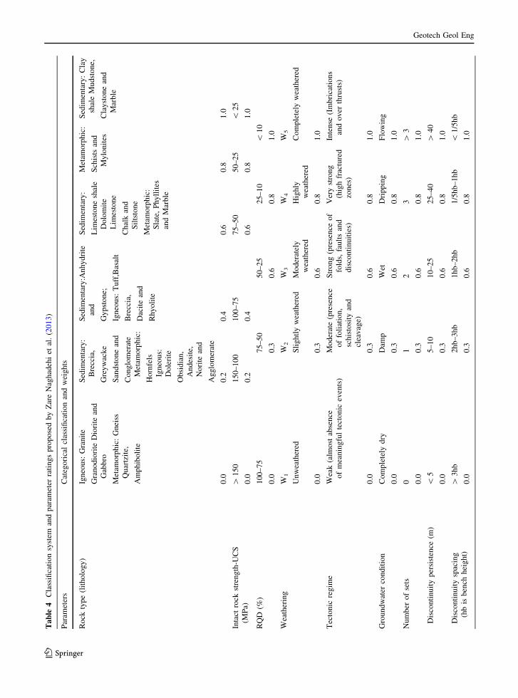
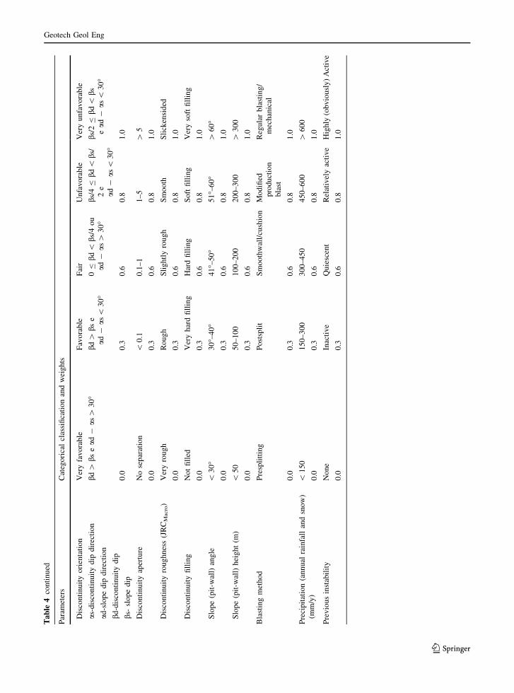
Zare Naghadehi et al. (2013) used a rating system to

classify the collected information into classes. This

rating system is presented in Table 4. The rating of

each variable varies between 0 and 1 and it is directly

related to the slope instability. In other words, higher

weights are assigned to values that lead to a higher

degree of slope instability than lower ones.

Table 2 Information of studied slopes, according to Zare Naghadehi et al. (2013)

Number of slopes Country Mine Number of slopes Country Mine

4 Iran Angooran 5 Australia Cadia-Hill

5 Iran Chadormalou 6 Sweden Aitik

5 Iran Choghart 7 Chile Escondida

4 Iran Golegohar 5 Spain Aznalcollar

4 Iran Sarcheshmeh 5 USA Betze-Post, Goldstrike

4 Iran Sungun 2 Spain La Yesa

7 South Africa Venetia 1 Chile Ujina, Collahuasi

5 Brazil Aguas Claras 1 Canada Panda, Ekati

5 Chile Chuquicamata 1 USA Esperanza, Phelps-Dosge

6 South Africa Sandsloot 2 Papua New Guine Ok-Tedi

Table 3 Database

geotechnical parameters,

according to Zare

Naghadehi et al. (2013)

Variable Name Nature Type Unit

V1 Rock type Overall environment Qualitative Lithology

V2 Intact rock strength Rock quality Quantitative MPa

V3 RQD Rock mass properties Quantitative %

V4 Weathering Qualitative Classification

V5 Tectonic Regime In-situ rock stress Qualitative Classification

V6 Groundwater Hydraulic conditions Qualitative Classification

V7 Number of sets Discontinuity properties Qualitative Unit

V8 Persistence Quantitative Meters

V9 Spacing Quantitative Meters

V10 Orientation Quantitative Degrees

V11 Aperture Quantitative Millimeters

V12 Roughness Qualitative Classification JRC

V13 Filling Qualitative Classification

V14 Overall Angle Pit-wall geometry Quantitative Degrees

V15 Overall Height Quantitative Meters

V16 Blasting method Construction Qualitative Type

V17 Precipitation Overall environment Qualitative Millimeters/year

V18 Previous Instability History Qualitative Classification

123

Geotech Geol Eng

Table

4Classificationsystem

andparam

eter

ratingsproposedbyZareNaghadehiet

al.(2013)

Param

eters

Categoricalclassificationandweights

Rock

type(lithology)

Igneous:

Granite

Granodiorite

Diorite

and

Gabbro

Metam

orphic:Gneiss

Quartzite,

Amphibolite

Sedim

entary:

Breccia,

Greywacke

Sandstoneand

Conglomerate

Metam

orphic:

Hornfels

Igneous:

Dolerite

Obsidian,

Andesite,

Norite

and

Agglomerate

Sedim

entary:Anhydrite

and

Gypstone;

Igneous:

Tuff,Basalt

Breccia,

Daciteand

Rhyolite

Sedim

entary:

Lim

estoneshale

Dolomite

Lim

estone

Chalkand

Siltstone

Metam

orphic:

Slate,Phyllites

andMarble

Metam

orphic:

Schists

and

Mylonites

Sedim

entary:Clay

shaleMudstone,

Claystoneand

Marble

0.0

0.2

0.4

0.6

0.8

1.0

Intact

rock

strength-U

CS

(MPa)

[150

150–100

100–75

75–50

50–25

\25

0.0

0.2

0.4

0.6

0.8

1.0

RQD

(%)

100–75

75–50

50–25

25–10

\10

0.0

0.3

0.6

0.8

1.0

Weathering

W1

W2

W3

W4

W5

Unweathered

Slightlyweathered

Moderately

weathered

Highly

weathered

Completely

weathered

0.0

0.3

0.6

0.8

1.0

Tectonic

regim

eWeak(alm

ostabsence

ofmeaningfultectonic

events)

Moderate(presence

offoliation,

schistosity

and

cleavage)

Strong(presence

of

folds,faultsand

discontinuities)

Verystrong

(highfractured

zones)

Intense

(Imbrications

andover

thrusts)

0.0

0.3

0.6

0.8

1.0

Groundwater

condition

Completely

dry

Dam

pWet

Dripping

Flowing

0.0

0.3

0.6

0.8

1.0

Number

ofsets

01

23

[3

0.0

0.3

0.6

0.8

1.0

Discontinuitypersistence

(m)

\5

5–10

10–25

25–40

[40

0.0

0.3

0.6

0.8

1.0

Discontinuityspacing

(hbisbench

height)

[3hb

2hb–3hb

1hb–2hb

1/5hb–1hb

\1/5hb

0.0

0.3

0.6

0.8

1.0

123

Geotech Geol Eng

Table

4continued

Param

eters

Categoricalclassificationandweights

Discontinuityorientation

as-discontinuitydip

direction

ad-slopedip

direction

bd-discontinuitydip

bs-

slopedip

Veryfavorable

Favorable

Fair

Unfavorable

Veryunfavorable

bd[

bsead

-as[

30�

bd[

bse

ad-

as\

30�

0B

bd\

bs/4

ou

ad-

as[

30�

bs/4

Bbd

\bs/

2e

ad-

as\

30�

bs/2

Bbd\

bsead

-as

\30�

0.0

0.3

0.6

0.8

1.0

Discontinuityaperture

Noseparation

\0.1

0.1–1

1–5

[5

0.0

0.3

0.6

0.8

1.0

Discontinuityroughness(JRCMacro)

Veryrough

Rough

Slightlyrough

Smooth

Slickensided

0.0

0.3

0.6

0.8

1.0

Discontinuityfilling

Notfilled

Veryhardfilling

Hardfilling

Softfilling

Verysoftfilling

0.0

0.3

0.6

0.8

1.0

Slope(pit-w

all)angle

\30�

30�–40�

41�–50�

51�–60�

[60�

0.0

0.3

0.6

0.8

1.0

Slope(pit-w

all)height(m

)\

50

50–100

100–200

200–300

[300

0.0

0.3

0.6

0.8

1.0

Blastingmethod

Presplitting

Postsplit

Smoothwall/cushion

Modified

production

blast

Regularblasting/

mechanical

0.0

0.3

0.6

0.8

1.0

Precipitation(annual

rainfallandsnow)

(mm/y)

\150

150–300

300–450

450–600

[600

0.0

0.3

0.6

0.8

1.0

Previousinstability

None

Inactive

Quiescent

Relativelyactive

Highly

(obviously)Active

0.0

0.3

0.6

0.8

1.0

123

Geotech Geol Eng

4.2 Application of Multivariate Statistics

4.2.1 Principal Component Analysis

The first part of the methodology was the application

of the principal component analysis in training sample

1. This technique allowed the transformation of

original qualitative variables into quantitative ones;

the scores of the principal components. This transfor-

mation was necessary because the boosting procedure

via discriminant analysis can only be accomplished in

a quantitative database. Table 5 presents the signifi-

cance of the 18 estimated components.

The first component explained 22.9% of the total

variance of the database; the second principal com-

ponent explained 13.2% of the total variance and so

forth. It is important to highlight that approximately

70% of the total variance of the database is explained

by the first six principal components.

Kaiser’s criterion (1958) was used to reduce the

database dimension. The principal components that

presented eigenvalues greater than one were selected,

i.e., the linear combinations that explained at least the

amount of variance of one original standardized vari-

able. Figure 6 presents the scree-plot for the first ten

principal components. According to Kaiser’s criterion

the first six principal components should be kept.

Figure 7 shows the relation between the first two

principal components which accounted for 36.0% of

the total database variability. Different symbols for

stable and unstable slopes were used in Fig. 7. It is

evident by observing Fig. 7 that the first principal

component was directly related to the stability status

condition of each slope. Slopes with positive scores in

the first principal component have a stable status and

slopes with negative scores have an unstable status. It

was correct for 71 slopes of the 75 analyzed,

representing an accuracy of 94.67%, so an error of

5.33%.

The set of variables with higher weights in the first

component are the slope height, blasting method,

previous instability, precipitation, weathering grade of

the rock and orientation of discontinuities. This is in a

good accordance with the results of systems analyzed

by Zare Naghadehi et al. (2013) in which most of the

selected parameters of current research have shown

high interaction intensity values and hence high

importance in the subject of slope stability.

Table 5 Significance of

the components and

proportion of explained

variance

Components Standard deviation Proportion of explained variance

By component Accumulated

Comp. 1 2.029 0.229 0.229

Comp. 2 1.54 0.132 0.360

Comp. 3 1.378 0.105 0.466

Comp. 4 1.253 0.087 0.553

Comp. 5 1.107 0.068 0.621

Comp. 6 1.006 0.056 0.677

Comp. 7 0.964 0.052 0.729

Comp. 8 0.958 0.051 0.780

Comp. 9 0.854 0.040 0.820

Comp. 10 0.779 0.034 0.854

Comp. 11 0.702 0.027 0.881

Comp. 12 0.674 0.025 0.907

Comp. 13 0.624 0.022 0.928

Comp. 14 0.595 0.020 0.948

Comp. 15 0.573 0.018 0.966

Comp. 16 0.497 0.014 0.980

Comp. 17 0.457 0.012 0.992

Comp. 18 0.388 0.008 1.000

123

Geotech Geol Eng

In the second component the variables with higher

weights are: the rock type, slope angle and the tectonic

regime.

The first two components account for 36.0% of the

total variability of the database. The meaning of the

other four selected principal component was not

straightforwardly interpreted.

4.2.2 Boosting Procedure via Discriminant Analysis

for Two Classes: Stable and Unstable

The discriminant analysis was used to determine the

starting basic classifier for the boosting procedure. A

number of 100 iterations for the stabilization of the

classifier were defined in the boosting procedure. The

procedure stabilized the classifiers in the seventh

iteration. Figure 8 shows the iterations and classifier

values.

The analysis of Fig. 8 allows observing the relation

between the values of the classifiers in each iteration.

The value of the classifier for coefficient 1 is greater

than the values of classifiers for the other coefficients

because of the variance explained by the first compo-

nent is 0.229 (see Table 5). This variance is high

comparing to the variance of other components; so the

first component explains significant part of the original

Fig. 6 Scree-plot of the first ten principal components

-4

-3

-2

-1

0

1

2

3

4

-6 -4 -2 0 2 4 6

2ª p

rinci

pal c

ompo

nent

- PC

2

1ª principal component - PC1

Graph of the principal component scores PC1 x PC2

OF OF - Unstable slope

Fig. 7 Scores of the first

two principal components

123

Geotech Geol Eng

data set variability, which reflects on a greater weight

of its classifier. As the values of the variances

explained by the other components are close, the

classifiers presented a slight variation.

Figure 9 presents the values of the constant cm for

each iteration of the boosting procedure. It is observed

that nearby the sixth iteration the constant value

became null, demonstrating the stabilization of

classifiers.

Once classifiers are stabilized, the final classifier is

defined by its result after six iterations. It is given by

the linear combination of classifiers fm, Eq. (12), i.e.

sign F xð Þð Þ ¼ signPM

m¼1cmfm xð Þ.

sign F xð Þð Þ ¼ 745:97 Comp1ð Þ þ 118:40 Comp2ð Þþ 78:14 Comp3ð Þ þ 46:31 Comp4ð Þ� 70:55 Comp5ð Þ � 54:85 Comp6ð Þ

ð12Þ

The sign of the function in Eq. (12), negative or

positive, indicates the classification status of the slope.

When the sign is negative, the slope is stable and when

the sign is positive, the slope is unstable. Figure 10

presents the errors related to the classification in each

iteration. It is possible to see that the larger error is

equal to 0.14 in the third iteration. The error stabilized

at the fifth iteration.

By observing Eq. (12) it is possible to see that the

largest classifiers are related to the first two compo-

nents. This result demonstrated that the classifiers of

the components 1 and 2 define the slope stability

condition status, confirming the results yielded by

principal component analysis.

4.2.3 Validation Results of the Function Obtained

by the Boosting via Discriminant Analysis

for Two Classes:

Stable and Unstable Conditions

The validation sample (Fig. 2) was used to perform the

internal validation. Table 6 presents the results of this

internal validation. The point estimates of the apparent

error rate, the overall probability of success, error 1

(probability of an unstable slope be classified as

stable) and error 2 (probability of a stable slope be

classified as unstable) are shown.

The overall probability of success is 94.73% in the

database used for internal validation. Consequently,

the apparent error rate is 5.26%. The errors 1 and 2 are

0 and 10.0%, respectively. This result, once again,

demonstrated the reliability of the method.

For this research, the two errors are important but

the error 1 is more serious. The error 1 occurs when an

unstable slope is classified as a stable slope. This error

Fig. 8 Relationship between iterations and classifier values

Fig. 9 Relationship between constant cm and each iteration

Fig. 10 Error rate of the boosting procedure

123

Geotech Geol Eng

could lead to safety problems in open pit slopes. The

error 2 occurs when a stable slope is classified as an

unstable slope. This error denotes a conservative

estimation of the slope stability status.

The error 1 is close to zero, which is in favor of

security. The error 2 is equal to 10.0%. Therefore, the

function obtained by boosting procedure via discrim-

inant analysis proved to be little conservative, once

error 2 comprised the total error rate of the function.

The bootstrap technique was used to estimate the

confidence intervals for the apparent error rate, the

overall probability of success, the error 1 and the error

2, Efron and Tibshirani (1993). In this technique

10,000 samples were randomly picked from the

validation sample (Fig. 4).

The confidence interval results provided the esti-

mation of the lower and upper limits of the apparent

error rate, the overall probability of success and the

errors 1 and 2. Table 7 shows the results of the

confidence intervals.

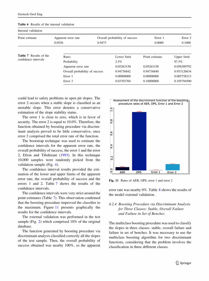
The confidence intervals were very strict around the

point estimates (Table 7). This observation confirmed

that the boosting procedure improved the classifier to

the maximum. Figure 11 presents graphically the

results for the confidence intervals.

The external validation was performed in the test

sample (Fig. 2) which comprised 10% of the original

database.

The function generated by boosting procedure via

discriminant analysis classified correctly all the slopes

of the test sample. Then, the overall probability of

success obtained was nearby 100%, so the apparent

error rate was nearby 0%. Table 8 shows the results of

the model external validation.

4.2.4 Boosting Procedure via Discriminant Analysis

for Three Classes: Stable, Overall Failure

and Failure in Set of Benches

Themulticlass boosting procedure was used to classify

the slopes in three classes: stable, overall failure and

failure in set of benches. It was necessary to use the

multiclass boosting algorithm for two discriminant

functions, considering that the problem involves the

classification in three different classes.

Table 6 Results of the internal validation

Internal validation

Point estimate Apparent error rate Overall probability of success Error 1 Error 2

0.0526 0.9473 0.0000 0.1000

Table 7 Results of the

confidence intervalsRates Lower limit Point estimate Upper limit

Probability 2.5% 97.5%

Apparent error rate 0.05263158 0.05263158 0.058389792

Overall probability of success 0.94736842 0.94736840 0.953126634

Error 1 0.00000000 0.00000000 0.005758213

Error 2 0.03703704 0.10000000 0.105794500

Fig. 11 Rates of AER, OPS, error 1 and error 2

123

Geotech Geol Eng

The multiclass boosting procedure was performed

with a number of 1000 iterations, but in the second

iteration the strongest classifiers were achieved. Thus,

after the second iteration classifiers do not change

anymore. The Eqs. 13 and 14 were obtained in the

second iteration:

FLD1 xð Þ ¼ �63:56 Comp1ð Þ þ 14:65 Comp2ð Þþ 14:71 Comp3ð Þ � 4:83 Comp4ð Þ� 5:44 Comp5ð Þ � 1:56 Comp6ð Þ ð13Þ

FLD2 xð Þ ¼ �3:74 Comp1ð Þ � 14:66 Comp2ð Þ� 13:49 Comp3ð Þ � 17:20 Comp4ð Þ� 18:98 Comp5ð Þ � 32:66 Comp6ð Þ ð14Þ

4.2.5 Validation Results of the Function Obtained

by the Boosting via Discriminant Analysis

for Three Classes: Stable, Overall Failure

and Failure in Set of Benches

The validation sample (Fig. 2) was used to perform the

internal validation. In this validation, there are six

types of errors:

1. Error 1: probability of a failure in set of benches

be classified as an overall failure

2. Error 2: probability of a failure in set of benches

be classified as a stable slope

3. Error 3: probability of an overall failure be

classified as a failure in set of benches

4. Error 4: probability of an overall failure be

classified as a stable slope

5. Error 5: probability of a stable slope be classified

as a failure in set of benches

6. Error 6: probability of a stable slope be classified

as an overall failure slope

Table 9 presents the results of the internal valida-

tion. The point estimates of the apparent error rate, the

overall probability of success and the six types of

errors are shown.

The overall probability of success is 68.45%. This

value is less than the value for the boosting with two

classes, probably due to the inclusion of one more

class. Figure 12 shows the comparison between

apparent error rate and overall probability of success

for the two analyses, with two classes and three

classes.

The apparent error rate is 31.57%. This value is

large comparing to the one obtained by boosting

procedure with two classes.

It is important to note that errors 1, 2 and 5 are

relative, and these probabilities are calculated accord-

ing to the number of slopes that are randomly selected

for the internal validation sample. In this validation the

algorithm selected 5 slopes of the class Failure in set of

benches and 4 of these slopes were classified by the

algorithm as Overall failure class and 1 slope as

Stable class. Therefore, Error 1 has a value of 80% and

Error 2 has a value of 20%, which reflects a lack of

accuracy of the boosting multiclass to distinguish the

failure in set of benches.

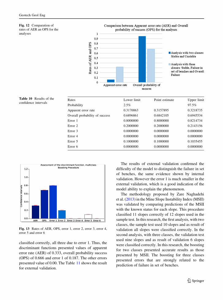
The confidence interval results provided the esti-

mation of the lower and upper limits of the apparent

error rate, the overall probability of success and the

errors 1, 2, 3, 4, 5 and 6. The range of values of the

confidence intervals is low; hence the point estimate is

significant. Table 10 shows the results of the confi-

dence intervals, and Fig. 13 presents the results for the

confidence intervals.

In the external validation, nine slopes of the sample

test (Fig. 2) were used, and three slopes were not

Table 8 Results of the model external validation

External validation

Point estimate Apparent error rate Overall probability of success Error 1 Error 2

0.0000 1.0000 0.0000 0.0000

Table 9 Results of the internal validation

Internal Validation for the analysis with three classes

Point estimate Apparent error rate Overall probability of success Error1 Error 2 Error 3 Error 4 Error 5 Error 6

0.3157 0.6842 0.8000 0.2000 0.0000 0.0000 0.1000 0.0000

123

Geotech Geol Eng

classified correctly, all three due to error 1. Thus, the

discriminant functions presented values of apparent

error rate (AER) of 0.333, overall probability success

(OPS) of 0.666 and error 1 of 0.187. The other errors

presented value of 0.00. The Table 11 shows the result

for external validation.

The results of external validation confirmed the

difficulty of the model to distinguish the failure in set

of benches, the same evidence shown by internal

validation. However the error 1 is much smaller in the

external validation, which is a good indication of the

model ability to explain the phenomenon.

The methodology proposed by Zare Naghadehi

et al. (2013) in theMine Slope Instability Index (MSII)

was validated by comparing predictions of the MSII

with the known status for each slope. This procedure

classified 11 slopes correctly of 12 slopes used in the

sample test. In this research, the first analysis, with two

classes, the sample test used 10 slopes and as result of

validation all slopes were classified correctly. In the

second analysis, with three classes, the validation test

used nine slopes and as result of validation 6 slopes

were classified correctly. In this research, the boosting

for two classes presented accurate results as those

presented by MSII. The boosting for three classes

presented errors that are strongly related to the

prediction of failure in set of benches.

Table 10 Results of the

confidence intervalsRates Lower limit Point estimate Upper limit

Probability 2.5% 97.5%

Apparent error rate 0.3170063 0.3157895 0.3218735

Overall probability of success 0.6896861 0.6842105 0.6945534

Error 1 0.8000000 0.8000000 0.8214734

Error 2 0.2000000 0.2000000 0.2143156

Error 3 0.0000000 0.0000000 0.0000000

Error 4 0.0000000 0.0000000 0.0000000

Error 5 0.1000000 0.1000000 0.1035455

Error 6 0.0000000 0.0000000 0.0000000

Fig. 12 Comparation of

rates of AER an OPS for the

analyses

Fig. 13 Rates of AER, OPS, error 1, error 2, error 3, error 4,

error 5 and error 6

123

Geotech Geol Eng

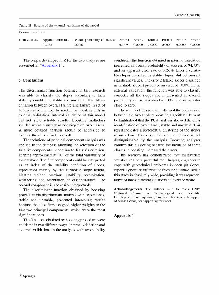
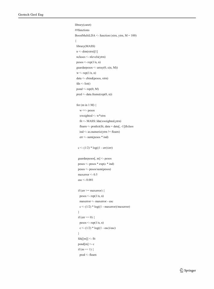
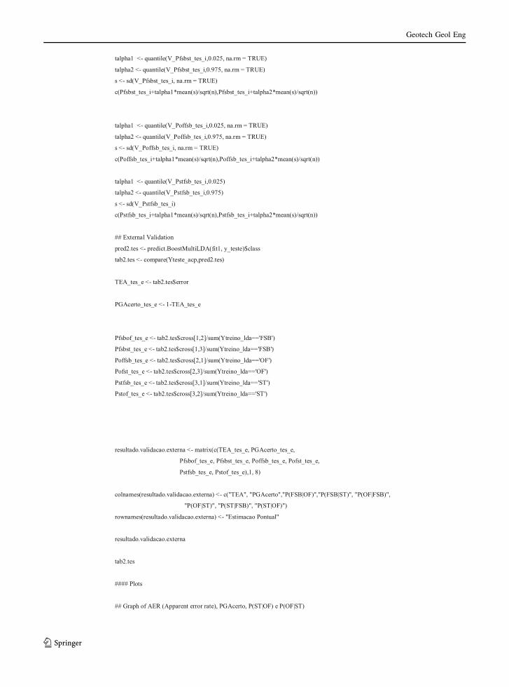
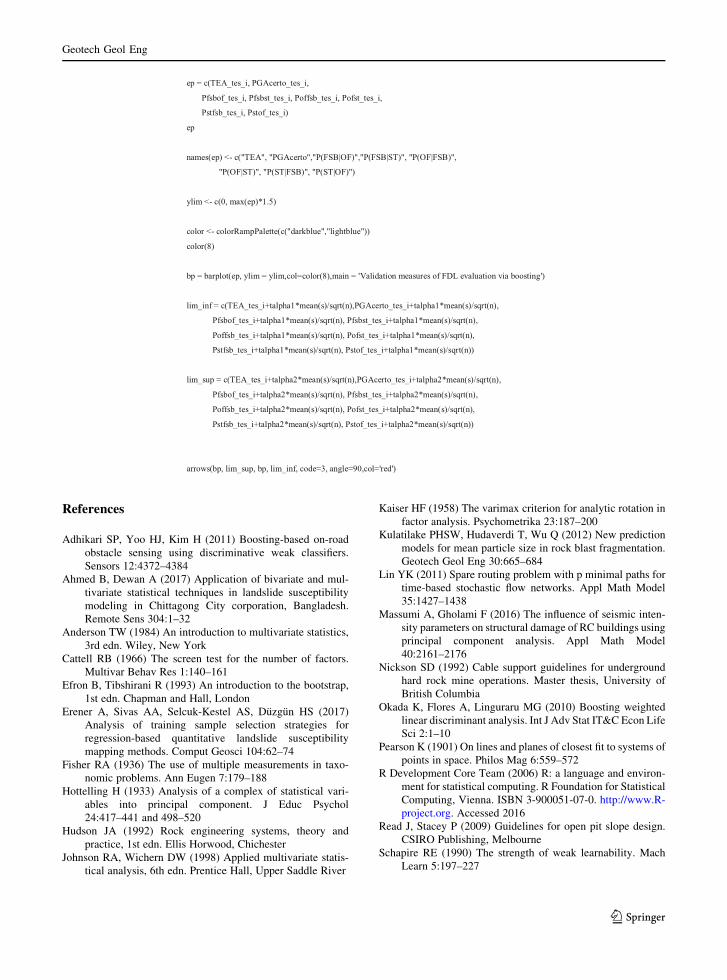
The scripts developed in R for the two analyses are

presented in ‘‘Appendix 1’’.

5 Conclusions

The discriminant function obtained in this research

was able to classify the slopes according to their

stability conditions, stable and unstable. The differ-

entiation between overall failure and failure in set of

benches is perceptible by multiclass boosting only in

external validation. Internal validation of this model

did not yield reliable results. Boosting multiclass

yielded worse results than boosting with two classes.

A more detailed analysis should be addressed to

explore the causes for this result.

The technique of principal component analysis was

applied to the database allowing the selection of the

first six components, according to Kaiser’s criterion,

keeping approximately 70% of the total variability of

the database. The first component could be interpreted

as an index of the stability condition of slopes,

represented mainly by the variables: slope height,

blasting method, previous instability, precipitation,

weathering and orientation of discontinuities. The

second component is not easily interpretable.

The discriminant function obtained by boosting

procedure via discriminant analysis with two classes,

stable and unstable, presented interesting results

because the classifiers assigned higher weights to the

first two principal components, which were the most

significant ones.

The functions obtained by boosting procedure were

validated in two different ways: internal validation and

external validation. In the analysis with two stability

conditions the function obtained in internal validation

presented an overall probability of success of 94.73%

and an apparent error rate of 5.26%. Error 1 (unsta-

ble slopes classified as stable slopes) did not present

significant values. The error 2 (stable slopes classified

as unstable slopes) presented an error of 10.0%. In the

external validation, the function was able to classify

correctly all the slopes and it presented an overall

probability of success nearby 100% and error rates

close to zero.

The results of this research allowed the comparison

between the two applied boosting algorithms. It must

be highlighted that the PCA analysis allowed the clear

identification of two classes, stable and unstable. This

result indicates a preferential clustering of the slopes

in only two classes, i.e. the scale of failure is not

distinguishable by the analysis. Boosting analyses

confirm this clustering because the inclusion of three

classes in boosting increased the errors.

This research has demonstrated that multivariate

statistics can be a powerful tool, helping engineers to

cope with geotechnical problems in open pit slopes,

especially because information fromthedatabaseused in

this study is absolutely wide, providing it was represen-

tative of many different situations all over the world.

Acknowledgements The authors wish to thank CNPq

(National Counsel of Technological and Scientific

Development) and Fapemig (Foundation for Research Support

of Minas Gerais) for supporting this work.

Appendix 1

Table 11 Results of the external validation of the model

External validation

Point estimate Apparent error rate Overall probability of success Error 1 Error 2 Error 3 Error 4 Error 5 Error 6

0.3333 0.6666 0.1875 0.0000 0.0000 0.0000 0.0000 0.0000

123

Geotech Geol Eng

SCRIPT FOR TWO CLASSES, STABLE AND UNSTABLE

## Algorithm Boosting via Discriminant Analysis ## install.packages('ks',dependencies=TRUE) library('ks')

## Discriminant function flda <- function(xtrain, group) { train <- cbind(xtrain, group) x1 <- as.matrix(train[group==-1, 1:(dim(train)[2]-1)]) x2 <- as.matrix(train[group==1, 1:(dim(train)[2]-1)]) mean_x1 <- apply(x1, 2, mean) mean_x2 <- apply(x2, 2, mean) S1 <- cov(x1)S2 <- cov(x2) Sc <- (((dim(x1)[1]-1)*S1)+((dim(x2)[1]-1)*S2))/(dim(x1)[1]+dim(x2)[1]-2)l_hat <- t(mean_x1 - mean_x2) %*% solve(Sc)m_hat <- .5 * t(mean_x1 - mean_x2) %*% solve(Sc) %*% (mean_x1 + mean_x2) means <- rbind(mean_x1, mean_x2) rownames(means) <- list("group 1 ", "group 2 ") result <- list(means, S1, S2, Sc, l_hat, m_hat) names(result) <- list("means", "s1", "s2", "sc", "coef", "threshold") result

}

## Discriminant function prediction predict.lda <- function(fit, newdata) { x <- newdata n <- dim(x)[1] coef <- fit$coefthreshold <- fit$threshold y_hat <- numeric(n) class <- numeric(n) for(t in 1:n) {

y_hat[t] <- coef%*%x[t,] if(y_hat[t]>=threshold)

class[t] <- -1 else

class[t] <- 1 } class

}

## Boosting via discriminant linear Fisher function BoostLDA <- function(xtrn, ytrn, M) { N <- dim(xtrn)[1] p <- dim(xtrn)[2] w <- rep((1/N),N) f.trn <- matrix(0,N,M) F.trn <- numeric(N) I <- matrix(0,N,M) error <- numeric(M) c <- numeric(M)coefs <- matrix(0,M,p) thresholds <- numeric(M) for (m in 1:M) { xweighted <- w*xtrn classifier <- flda(xweighted,ytrn) coefs[m,] <- classifier$coef thresholds[m] <- classifier$threshold f.trn[,m] <- predict.lda(classifier,xtrn) I[,m] <- (f.trn[,m] != ytrn) error[m] <- w%*%I[,m] c[m] <- .5*log((1-error[m])/error[m]) w <- w*exp(-c[m]*ytrn*f.trn[,m]) w <- pmax(w/sum(w),1e-24)

123

Geotech Geol Eng

F.trn <- F.trn+(c[m]*f.trn[,m]) } class.trn <- sign(F.trn) result <- list(coefs, thresholds, error, w, c, class.trn, error.trn = apply(I, 2, mean)) names(result) <- list("coefs", "thresholds", "error","weights", "const", "class.trn", "error.trn") result

}

## boosting to predict discriminant function predict.boostlda <- function(fit, newdata) { x <- newdata n <- dim(x)[1] p <- dim(x)[2]coefs <- fit$coefs thresholds <- fit$thresholds boost.weights <- fit$const M <- length(thresholds) y_hat <- matrix(0,n,M) class <- matrix(0,n,M) for (i in 1:M) { for (j in 1:n) {

y_hat[j,i] <- coefs[i, ]%*%x[j, ] if (y_hat[j,i] >= thresholds[i]) class[j,i] <- -1 else class[j,i] <- 1

} } class.final <- sign(t(t(boost.weights)%*%t(class))) result <- list(class, class.final) names(result) <- list("class", "class.final") result

}

########## Boosting estimation start

dados = read.table("dados_allan.txt",header=TRUE,row.names=1) head(dados)

n = dim(dados)[1]

## PCA analysis with 90% of data; 10% to test FDA prop = 0.9

## Sample to estimate PCA set.seed(1234) trind_acp = sample(1:n, floor(prop*n),replace = FALSE) Xtreino_acp = dados[trind_acp,-19]Ytreino_acp = dados[trind_acp,19]

## Sample for external validation teind_acp = setdiff(1:n,trind_acp) Xteste_acp = dados[teind_acp,-19]Yteste_acp = dados[teind_acp,19] Yteste_acp_cod = ifelse(Yteste_acp=='ST',-1,1)

## Estimation of PCA components acp = princomp(Xtreino_acp, cor = TRUE, scores=TRUE) y_acp = acp$scores[,1:6] y_acp

## Sample to external validation y_teste = predict(acp,Xteste_acp)[,1:6] y_teste

## Boosting function estiomation via discriminant analysis

## Training sample m = dim(y_acp)[1] prop_lda = 0.75

set.seed(432100) trind_lda = sample(1:m, floor(prop_lda*m),replace = FALSE) Xtreino_lda = y_acp[trind_lda,]

123

Geotech Geol Eng

Ytreino_lda = Ytreino_acp[trind_lda] Ytreino_lda_cod = ifelse(Ytreino_lda=='ST',-1,1)

## Sample to test FDA, internal cross validation teind_lda = setdiff(1:m,trind_lda) Xteste_lda = y_acp[teind_lda,] Yteste_lda = Ytreino_acp[teind_lda] Yteste_lda_cod = ifelse(Yteste_lda=='ST',-1,1)

## Boosting model estimation via discrimant function M <- 100fit1 <- BoostLDA(Xtreino_lda, Ytreino_lda_cod,M)

## AER estimation: Sample for punctual validation pred1.tes <- predict.boostlda(fit1, Xteste_lda)$class.final tab1.tes <- compare(pred1.tes, Yteste_lda_cod)

TEA_tes_i <- tab1.tes$error PGAcerto_tes_i <- 1-TEA_tes_i Pstof_tes_i <- tab1.tes$cross[2,1]/sum(Ytreino_lda_cod==1) Pofst_tes_i <- tab1.tes$cross[1,2]/sum(Ytreino_lda_cod==-1)

resultado.validacao.interna <- matrix(c(TEA_tes_i, PGAcerto_tes_i, Pstof_tes_i, Pofst_tes_i),1, 4)

colnames(resultado.validacao.interna) <- c("TEA", "PGAcerto","P(ST|OF)","P(OF|ST)") rownames(resultado.validacao.interna) <- "Estimacao Pontual"

resultado.validacao.interna

### Confidence interval estimation - bootstrap

B = 10000

V_TEA_tes_i = matrix(NA,B,1) V_PGAcerto_tes_i = matrix(NA,B,1) V_Pstof_tes_i = matrix(NA,B,1) V_Pofst_tes_i = matrix(NA,B,1)

for(i in 1:B){

## CI for boosting, internal validation teind_lda_boot = sample(teind_lda, length(teind_lda),replace = TRUE) Xteste_lda_boot = y_acp[teind_lda_boot,] Yteste_lda_boot = Ytreino_acp[teind_lda_boot]Yteste_lda_boot_cod = ifelse(Yteste_lda_boot=='ST',-1,1)

pred1.tes <- predict.boostlda(fit1, Xteste_lda_boot)$class.final tab1.tes <- compare(pred1.tes, Yteste_lda_boot_cod) V_TEA_tes_i[i] <- tab1.tes$errorV_PGAcerto_tes_i[i] <- 1-V_TEA_tes_i[i] V_Pstof_tes_i[i] <- tab1.tes$cross[2,1]/sum(Yteste_lda_boot_cod==1)V_Pofst_tes_i[i] <- tab1.tes$cross[1,2]/sum(Yteste_lda_boot_cod==-1)

}

## confidence interval via resampling

talpha1 <- quantile(V_TEA_tes_i,0.025) talpha2 <- quantile(V_TEA_tes_i,0.975) s <- sd(V_TEA_tes_i) c(TEA_tes_i+talpha1*mean(s)/sqrt(n),TEA_tes_i+talpha2*mean(s)/sqrt(n))

talpha1 <- quantile(V_PGAcerto_tes_i,0.025) talpha2 <- quantile(V_PGAcerto_tes_i,0.975) s <- sd(V_PGAcerto_tes_i) c(PGAcerto_tes_i+talpha1*mean(s)/sqrt(n),PGAcerto_tes_i+talpha2*mean(s)/sqrt(n))

talpha1 <- quantile(V_Pstof_tes_i,0.025) talpha2 <- quantile(V_Pstof_tes_i,0.975) s <- sd(V_Pstof_tes_i)

123

Geotech Geol Eng

c(Pstof_tes_i+talpha1*mean(s)/sqrt(n),Pstof_tes_i+talpha2*mean(s)/sqrt(n))

talpha1 <- quantile(V_Pofst_tes_i,0.025) talpha2 <- quantile(V_Pofst_tes_i,0.975) s <- sd(V_Pofst_tes_i) c(Pofst_tes_i+talpha1*mean(s)/sqrt(n),Pofst_tes_i+talpha2*mean(s)/sqrt(n))

## External validation: test sampling pred2.tes <- predict.boostlda(fit1, y_teste)$class.final tab2.tes <- compare(pred2.tes, Yteste_acp_cod)

TEA_tes_e <- tab2.tes$error

PGAcerto_tes_e <- 1-TEA_tes_e

Pstof_tes_e <- tab2.tes$cross[2,1]/sum(Ytreino_lda_cod==1) Pofst_tes_e <- tab2.tes$cross[1,2]/sum(Ytreino_lda_cod==-1)

resultado.validacao.externa <- matrix(c(TEA_tes_e, PGAcerto_tes_e, Pstof_tes_e, Pofst_tes_e),1, 4)

colnames(resultado.validacao.externa) <- c("TEA", "PGAcerto","P(ST|OF)","P(OF|ST)") rownames(resultado.validacao.externa) <- "Estimacao Pontual"

resultado.validacao.externa

#### Drawing graphs with CI

## Graph of AER (Apparent error rate), PGAcerto, P(ST|OF) e P(OF|ST)

ep = c(TEA_tes_i, PGAcerto_tes_i, Pstof_tes_i, Pofst_tes_i) ep

names(ep) <- c('TEA', 'PGAcerto', 'P(ST|OF)','P(OF|ST)')

ylim <- c(0, max(ep)*1.5)

color <- colorRampPalette(c("darkblue","lightblue")) color(4)

bp = barplot(ep, ylim = ylim,col=color(4),main = 'Medidas de Avaliação da FDLF via Boosting')

lim_inf = c(TEA_tes_i+talpha1*mean(s)/sqrt(n),PGAcerto_tes_i+talpha1*mean(s)/sqrt(n), Pstof_tes_i+talpha1*mean(s)/sqrt(n),Pofst_tes_i+talpha1*mean(s)/sqrt(n))

lim_sup = c(TEA_tes_i+talpha2*mean(s)/sqrt(n),PGAcerto_tes_i+talpha2*mean(s)/sqrt(n), Pstof_tes_i+talpha2*mean(s)/sqrt(n),Pofst_tes_i+talpha2*mean(s)/sqrt(n))

arrows(bp, lim_sup, bp, lim_inf, code=3, angle=90,col='red')

SCRIPT FOR BOOSTING MULTICLASS

##final boosting multiclass##

########################

##packages##

library(ks)

library(MASS)

123

Geotech Geol Eng

library(caret)

##functions

BoostMultiLDA <- function (xtrn, ytrn, M = 100)

{

library(MASS)

n <- dim(xtrn)[1]

nclases <- nlevels(ytrn)

pesos <- rep(1/n, n)

guardarpesos <- array(0, c(n, M))

w <- rep(1/n, n)

data <- cbind(pesos, xtrn)

fds <- list()

pond <- rep(0, M)

pred <- data.frame(rep(0, n))

for (m in 1:M) {

w <<- pesos

xweighted <- w*xtrn

fit <- MASS::lda(xweighted,ytrn)

flearn <- predict(fit, data = data[, -1])$class

ind <- as.numeric(ytrn != flearn)

err <- sum(pesos * ind)

c <- (1/2) * log((1 - err)/err)

guardarpesos[, m] <- pesos

pesos <- pesos * exp(c * ind)

pesos <- pesos/sum(pesos)

maxerror <- 0.5

eac <- 0.001

if (err >= maxerror) {

pesos <- rep(1/n, n)

maxerror <- maxerror - eac

c <- (1/2) * log((1 - maxerror)/maxerror)

}

if (err == 0) {

pesos <- rep(1/n, n)

c <- (1/2) * log((1 - eac)/eac)

}

fds[[m]] <- fit

pond[m] <- c

if (m == 1) {

pred <- flearn

123

Geotech Geol Eng

}else {

pred <- data.frame(pred, flearn)

}

}

classfinal <- array(0, c(n, nlevels(ytrn)))

for (i in 1:nlevels(ytrn)) {

classfinal[, i] <- matrix(as.numeric(pred == levels(ytrn)[i]),

nrow = n) %*% as.vector(pond)

}

predclass <- rep("O", n)

predclass <- factor(apply(classfinal,1,which.max), labels=c(levels(ytrn)[1],levels(ytrn)[2],levels(ytrn)[3]),

levels=c(1,2,3))

probabilidades <- classfinal/apply(classfinal, 1, sum)

ans <- list(FD = fds, Importancia_cl = pond,

votos = classfinal, prob = probabilidades, class = predclass)

attr(ans, "Ytreino.summary") <- summary(ytrn, maxsum = 700)

ans$call <- match.call()

class(ans) <- "boosting"

ans

}

predict.BoostMultiLDA <- function (fit, newdata)

{

x <- newdata

n <- dim(x)[1]

p <- dim(x)[2]

ytrn.summary <- attributes(fit1)$Ytreino.summary

nclasses <- length(ytrn.summary)

pesos <- rep(1/n, n)

pond <- fit$Importancia_cl

M = length(fit$FD)

for (i in 1:M) {

prd <- predict(fit$FD[[i]],x)$class

if (i == 1) {

pred <- prd

}else {

pred <- data.frame(pred, prd)

}

}

classfinal <- array(0, c(n, nclasses))

for (i in 1:nclasses) {

classfinal[, i] <- matrix(as.numeric(pred == names(ytrn.summary)[i]),

nrow = n) %*% pond

}

predclass <- rep("O", n)

predclass <- factor(apply(classfinal,1,which.max), labels=c(names(ytrn.summary)[1],names(ytrn.summary)[2]

,names(ytrn.summary)[3]),

levels=c(1,2,3))

123

Geotech Geol Eng

prob <- classfinal/apply(classfinal, 1, sum)

output <- list( votos = classfinal, prob = prob, class = predclass)

}

Script

#########################################

########## Starting boosting estimation########

##########################################

dados = read.table("dados_allan_tres.txt",header=TRUE,row.names=1)

head(dados)

str(dados)

n = dim(dados)[1]

## Sample with 90%##

prop = 0.9

## Sample to estimate PCA

set.seed(1234)

trind_acp = sample(1:n, floor(prop*n),replace = FALSE)

Xtreino_acp = dados[trind_acp,-19]

Ytreino_acp = dados[trind_acp,19]

## Sample to test FDA: external validation

teind_acp = setdiff(1:n,trind_acp)

Xteste_acp = dados[teind_acp,-19]

Yteste_acp = dados[teind_acp,19]

#Yteste_acp_cod = ifelse(Yteste_acp=='ST',-1,1)

## Estimating PCA

acp = princomp(Xtreino_acp, cor = TRUE, scores=TRUE)

y_acp = acp$scores[,1:6]

y_acp

## Sample to external validation

y_teste = predict(acp,Xteste_acp)[,1:6]

y_teste

## Estimate boosting function with function discriminant

## Sample trainning

m = dim(y_acp)[1]

prop_lda = 0.75

set.seed(432100)

trind_lda = sample(1:m, floor(prop_lda*m),replace = FALSE)

Xtreino_lda = y_acp[trind_lda,]

123

Geotech Geol Eng

Ytreino_lda = Ytreino_acp[trind_lda]

#Ytreino_lda_cod = ifelse(Ytreino_lda=='ST',-1,1)

## Sample to internal validation

teind_lda = setdiff(1:m,trind_lda)

Xteste_lda = y_acp[teind_lda,]

Yteste_lda = Ytreino_acp[teind_lda]

#Yteste_lda_cod = ifelse(Yteste_lda=='ST',-1,1)

## Estimating boosting with discriminantfunction

M <- 1000

fit1 <- BoostMultiLDA(Xtreino_lda, Ytreino_lda,M)

## Estimating AER

pred1.tes <- predict.BoostMultiLDA(fit1, Xteste_lda)$class

tab1.tes <- compare(Yteste_lda, pred1.tes)

TEA_tes_i = tab1.tes$error

PGAcerto_tes_i <- 1-TEA_tes_i

Pfsbof_tes_i <- tab1.tes$cross[1,2]/sum(Yteste_lda=='FSB')

Pfsbst_tes_i <- tab1.tes$cross[1,3]/sum(Yteste_lda=='FSB')

Poffsb_tes_i <- tab1.tes$cross[2,1]/sum(Yteste_lda=='OF')

Pofst_tes_i <- tab1.tes$cross[2,3]/sum(Yteste_lda=='OF')

Pstfsb_tes_i <- tab1.tes$cross[3,1]/sum(Yteste_lda=='ST')

Pstof_tes_i <- tab1.tes$cross[3,2]/sum(Yteste_lda=='ST')

library(caret)

confusionMatrix(table(Yteste_lda,pred1.tes))

fit1$Importancia_cl

### Confidence interval

B = 10000

V_TEA_tes_i = matrix(NA,B,1)

V_PGAcerto_tes_i = matrix(NA,B,1)

V_Pfsbof_tes_i = matrix(NA,B,1)

V_Pfsbst_tes_i = matrix(NA,B,1)

V_Poffsb_tes_i = matrix(NA,B,1)

V_Pofst_tes_i = matrix(NA,B,1)

V_Pstfsb_tes_i = matrix(NA,B,1)

V_Pstof_tes_i = matrix(NA,B,1)

for(i in 1:B){

## IC bootstrap for boosting using internal validation

teind_lda_boot = sample(teind_lda, length(teind_lda),replace = TRUE)

123

Geotech Geol Eng

Xteste_lda_boot = y_acp[teind_lda_boot,]

Yteste_lda_boot = Ytreino_acp[teind_lda_boot]

# Yteste_lda_boot_cod = ifelse(Yteste_lda_boot=='ST',-1,1)

pred1.tes <- predict.BoostMultiLDA(fit1, Xteste_lda_boot)$class

tab1.tes <- compare(Yteste_lda_boot,pred1.tes)

V_TEA_tes_i[i] <- tab1.tes$error

V_PGAcerto_tes_i[i] <- 1-V_TEA_tes_i[i]

V_Pfsbof_tes_i[i] <- tab1.tes$cross[1,2]/sum(Yteste_lda_boot=='FSB')

V_Pfsbst_tes_i[i] <- tab1.tes$cross[1,3]/sum(Yteste_lda_boot=='FSB')

V_Poffsb_tes_i[i] <- tab1.tes$cross[2,1]/sum(Yteste_lda_boot=='OF')

V_Pofst_tes_i[i] <- tab1.tes$cross[2,3]/sum(Yteste_lda_boot=='OF')

V_Pstfsb_tes_i[i] <- tab1.tes$cross[3,1]/sum(Yteste_lda_boot=='ST')

V_Pstof_tes_i[i] <- tab1.tes$cross[3,2]/sum(Yteste_lda_boot=='ST')

print(i)

}

## confidence interval via resampling

talpha1 <- quantile(V_TEA_tes_i,0.025)

talpha2 <- quantile(V_TEA_tes_i,0.975)

s <- sd(V_TEA_tes_i)

c(TEA_tes_i+talpha1*s/sqrt(n),TEA_tes_i+talpha2*s/sqrt(n))

talpha1 <- quantile(V_PGAcerto_tes_i,0.025)

talpha2 <- quantile(V_PGAcerto_tes_i,0.975)

s <- sd(V_PGAcerto_tes_i)

c(PGAcerto_tes_i+talpha1*mean(s)/sqrt(n),PGAcerto_tes_i+talpha2*mean(s)/sqrt(n))

talpha1 <- quantile(V_Pstof_tes_i,0.025)

talpha2 <- quantile(V_Pstof_tes_i,0.975)

s <- sd(V_Pstof_tes_i)

c(Pstof_tes_i+talpha1*mean(s)/sqrt(n),Pstof_tes_i+talpha2*mean(s)/sqrt(n))

talpha1 <- quantile(V_Pofst_tes_i,0.025, na.rm = TRUE)

talpha2 <- quantile(V_Pofst_tes_i,0.975, na.rm = TRUE)

s <- sd(V_Pofst_tes_i, na.rm = TRUE)

c(Pofst_tes_i+talpha1*mean(s)/sqrt(n),Pofst_tes_i+talpha2*mean(s)/sqrt(n))

talpha1 <- quantile(V_Pfsbof_tes_i,0.025, na.rm = TRUE)

talpha2 <- quantile(V_Pfsbof_tes_i,0.975, na.rm = TRUE)

s <- sd(V_Pfsbof_tes_i, na.rm = TRUE)

c(Pfsbof_tes_i+talpha1*mean(s)/sqrt(n),Pfsbof_tes_i+talpha2*mean(s)/sqrt(n))

123

Geotech Geol Eng

talpha1 <- quantile(V_Pfsbst_tes_i,0.025, na.rm = TRUE)

talpha2 <- quantile(V_Pfsbst_tes_i,0.975, na.rm = TRUE)

s <- sd(V_Pfsbst_tes_i, na.rm = TRUE)

c(Pfsbst_tes_i+talpha1*mean(s)/sqrt(n),Pfsbst_tes_i+talpha2*mean(s)/sqrt(n))

talpha1 <- quantile(V_Poffsb_tes_i,0.025, na.rm = TRUE)

talpha2 <- quantile(V_Poffsb_tes_i,0.975, na.rm = TRUE)

s <- sd(V_Poffsb_tes_i, na.rm = TRUE)

c(Poffsb_tes_i+talpha1*mean(s)/sqrt(n),Poffsb_tes_i+talpha2*mean(s)/sqrt(n))

talpha1 <- quantile(V_Pstfsb_tes_i,0.025)

talpha2 <- quantile(V_Pstfsb_tes_i,0.975)

s <- sd(V_Pstfsb_tes_i)

c(Pstfsb_tes_i+talpha1*mean(s)/sqrt(n),Pstfsb_tes_i+talpha2*mean(s)/sqrt(n))

## External Validation

pred2.tes <- predict.BoostMultiLDA(fit1, y_teste)$class

tab2.tes <- compare(Yteste_acp,pred2.tes)

TEA_tes_e <- tab2.tes$error

PGAcerto_tes_e <- 1-TEA_tes_e

Pfsbof_tes_e <- tab2.tes$cross[1,2]/sum(Ytreino_lda=='FSB')

Pfsbst_tes_e <- tab2.tes$cross[1,3]/sum(Ytreino_lda=='FSB')

Poffsb_tes_e <- tab2.tes$cross[2,1]/sum(Ytreino_lda=='OF')

Pofst_tes_e <- tab2.tes$cross[2,3]/sum(Ytreino_lda=='OF')

Pstfsb_tes_e <- tab2.tes$cross[3,1]/sum(Ytreino_lda=='ST')

Pstof_tes_e <- tab2.tes$cross[3,2]/sum(Ytreino_lda=='ST')

resultado.validacao.externa <- matrix(c(TEA_tes_e, PGAcerto_tes_e,

Pfsbof_tes_e, Pfsbst_tes_e, Poffsb_tes_e, Pofst_tes_e,

Pstfsb_tes_e, Pstof_tes_e),1, 8)

colnames(resultado.validacao.externa) <- c("TEA", "PGAcerto","P(FSB|OF)","P(FSB|ST)", "P(OF|FSB)",

"P(OF|ST)", "P(ST|FSB)", "P(ST|OF)")

rownames(resultado.validacao.externa) <- "Estimacao Pontual"

resultado.validacao.externa

tab2.tes

#### Plots

## Graph of AER (Apparent error rate), PGAcerto, P(ST|OF) e P(OF|ST)

123

Geotech Geol Eng

References

Adhikari SP, Yoo HJ, Kim H (2011) Boosting-based on-road

obstacle sensing using discriminative weak classifiers.

Sensors 12:4372–4384

Ahmed B, Dewan A (2017) Application of bivariate and mul-

tivariate statistical techniques in landslide susceptibility

modeling in Chittagong City corporation, Bangladesh.

Remote Sens 304:1–32

Anderson TW (1984) An introduction to multivariate statistics,

3rd edn. Wiley, New York

Cattell RB (1966) The screen test for the number of factors.

Multivar Behav Res 1:140–161

Efron B, Tibshirani R (1993) An introduction to the bootstrap,

1st edn. Chapman and Hall, London

Erener A, Sivas AA, Selcuk-Kestel AS, Duzgun HS (2017)

Analysis of training sample selection strategies for

regression-based quantitative landslide susceptibility

mapping methods. Comput Geosci 104:62–74

Fisher RA (1936) The use of multiple measurements in taxo-

nomic problems. Ann Eugen 7:179–188

Hottelling H (1933) Analysis of a complex of statistical vari-

ables into principal component. J Educ Psychol

24:417–441 and 498–520

Hudson JA (1992) Rock engineering systems, theory and

practice, 1st edn. Ellis Horwood, Chichester

Johnson RA, Wichern DW (1998) Applied multivariate statis-

tical analysis, 6th edn. Prentice Hall, Upper Saddle River

Kaiser HF (1958) The varimax criterion for analytic rotation in

factor analysis. Psychometrika 23:187–200

Kulatilake PHSW, Hudaverdi T, Wu Q (2012) New prediction

models for mean particle size in rock blast fragmentation.

Geotech Geol Eng 30:665–684

Lin YK (2011) Spare routing problem with p minimal paths for

time-based stochastic flow networks. Appl Math Model

35:1427–1438

Massumi A, Gholami F (2016) The influence of seismic inten-

sity parameters on structural damage of RC buildings using

principal component analysis. Appl Math Model

40:2161–2176

Nickson SD (1992) Cable support guidelines for underground

hard rock mine operations. Master thesis, University of

British Columbia

Okada K, Flores A, Linguraru MG (2010) Boosting weighted

linear discriminant analysis. Int J Adv Stat IT&C Econ Life

Sci 2:1–10

Pearson K (1901) On lines and planes of closest fit to systems of

points in space. Philos Mag 6:559–572

R Development Core Team (2006) R: a language and environ-

ment for statistical computing. R Foundation for Statistical

Computing, Vienna. ISBN 3-900051-07-0. http://www.R-

project.org. Accessed 2016

Read J, Stacey P (2009) Guidelines for open pit slope design.

CSIRO Publishing, Melbourne

Schapire RE (1990) The strength of weak learnability. Mach

Learn 5:197–227

ep = c(TEA_tes_i, PGAcerto_tes_i,

Pfsbof_tes_i, Pfsbst_tes_i, Poffsb_tes_i, Pofst_tes_i,

Pstfsb_tes_i, Pstof_tes_i)

ep

names(ep) <- c("TEA", "PGAcerto","P(FSB|OF)","P(FSB|ST)", "P(OF|FSB)",

"P(OF|ST)", "P(ST|FSB)", "P(ST|OF)")

ylim <- c(0, max(ep)*1.5)

color <- colorRampPalette(c("darkblue","lightblue"))

color(8)

bp = barplot(ep, ylim = ylim,col=color(8),main = 'Validation measures of FDL evaluation via boosting')

lim_inf = c(TEA_tes_i+talpha1*mean(s)/sqrt(n),PGAcerto_tes_i+talpha1*mean(s)/sqrt(n),

Pfsbof_tes_i+talpha1*mean(s)/sqrt(n), Pfsbst_tes_i+talpha1*mean(s)/sqrt(n),

Poffsb_tes_i+talpha1*mean(s)/sqrt(n), Pofst_tes_i+talpha1*mean(s)/sqrt(n),

Pstfsb_tes_i+talpha1*mean(s)/sqrt(n), Pstof_tes_i+talpha1*mean(s)/sqrt(n))

lim_sup = c(TEA_tes_i+talpha2*mean(s)/sqrt(n),PGAcerto_tes_i+talpha2*mean(s)/sqrt(n),

Pfsbof_tes_i+talpha2*mean(s)/sqrt(n), Pfsbst_tes_i+talpha2*mean(s)/sqrt(n),

Poffsb_tes_i+talpha2*mean(s)/sqrt(n), Pofst_tes_i+talpha2*mean(s)/sqrt(n),

Pstfsb_tes_i+talpha2*mean(s)/sqrt(n), Pstof_tes_i+talpha2*mean(s)/sqrt(n))

arrows(bp, lim_sup, bp, lim_inf, code=3, angle=90,col='red')

123

Geotech Geol Eng

Skurichina M, Duin RPW (2000) Boosting in linear discrimi-

nant analysis. In: First international workshop on multiple

classifier systems, Cagliari

Wu X, Wu B, Sun J, Qiu S, Li X (2015) A hybrid fuzzy

K-harmonic means clustering algorithm. Appl MathModel

39:3398–3409

Wyllie DC, Mah CW (2004) Rock slope engineering, civil and

mining, 4th edn. Spon Press, Taylor & Francis Group,

London

Yilmaz Is-ık (2009) Landslide susceptibility mapping using

frequency ratio, logistic regression, artificial neural net-

works and their comparison: case study from Kat land-

slides (Tokat-Turkey). Comput Geosci 35:1125–1138

Zare Naghadehi M, Jimenez R, Khalokakaie R, Jalali SME

(2013) A new open-pit mine slope instability index defined

using the improved rock engineering systems approach. Int

J Rock Mech Min Sci 61:1–14

123

Geotech Geol Eng