EVALUATION OF QUALITY CONTROL PARAMETERS

FOR SUPERPAVE HOT MIX ASPHALT

John P. Zaniewski, Ph.D., P.E.

Thomas Adams

Asphalt Technology Program

Department of Civil and Environmental Engineering

Morgantown, West Virginia

April 2005

ii

NOTICE

The contents of this report reflect the views of the authors who are responsible for

the facts and the accuracy of the data presented herein. The contents do not necessarily

reflect the official views or policies of the State or the Federal Highway Administration.

This report does not constitute a standard, specification, or regulation. Trade or

manufacturer names which may appear herein are cited only because they are considered

essential to the objectives of this report. The United States Government and the State of

West Virginia do not endorse products or manufacturers. This report is prepared for the

West Virginia Department of Transportation, Division of Highways, in cooperation with

the US Department of Transportation, Federal Highway Administration.

iii

Technical Report Documentation Page

1. Report No. 2. Government

Association No.

3. Recipient's catalog No.

4. Title and Subtitle

Evaluation of Quality Control Parameters for

Superpave Hot Mix Asphalt

5. Report Date April, 2005

6. Performing Organization Code

7. Author(s)

John P. Zaniewski, Thomas Adams 8. Performing Organization Report No.

9. Performing Organization Name and Address

Asphalt Technology Program

Department of Civil and Environmental

Engineering

West Virginia University

P.O. Box 6103

Morgantown, WV 26506-6103

10. Work Unit No. (TRAIS)

11. Contract or Grant No.

12. Sponsoring Agency Name and Address

West Virginia Division of Highways

1900 Washington St. East

Charleston, WV 25305

13. Type of Report and Period Covered

14. Sponsoring Agency Code

15. Supplementary Notes

Performed in Cooperation with the U.S. Department of Transportation - Federal Highway

Administration

16. Abstract

Quality control tests used for the WVDOH QC/QA process are standard tests

published by both AASHTO and ASTM) By policy, each of these organizations includes

precision and bias statements as part of each test method. The variability associated with the

testing methodology should not influence the decision to accept or reject a material in the

QC/QA process.

The current QC/QA requirements used by the WVDOH for Superpave projects have

not been statistically evaluated to establish the risk to the agency and constructor for either

accepting an unsatisfactory material or rejecting a satisfactory material respectively. A

rigorous evaluation of these risks is difficult due to the interdependence of some of the quality

control parameters. However, a simulation method is available that can be used to identify

these risks.

This research evaluated the risk levels associated with the current methods of quality

control and acceptance used by the WVDOH for Superpave construction projects. Risk was

defined as the probability of the WVDOH accepting a substandard product or rejecting an

acceptable product. Through Monte Carlo simulation it was demonstrated that the QC/QA

procedures used by the state are acceptable with respect to the risk associated with acceptance

and rejection of materials. 17. Key Words

Asphalt construction, quality control, quality

assurance, Monte Carlo simulation

18. Distribution Statement

19. Security Classif. (of this

report)

Unclassified

20. Security Classif. (of

this page)

Unclassified

21. No. Of Pages 65

22. Price

Form DOT F 1700.7 (8-72) Reproduction of completed page authorized

iv

TABLE OF CONTENTS

Chapter 1 Introduction .........................................................................................................1

1.1 Problem Statement .........................................................................................................2

1.2 Research Objective ........................................................................................................2

1.3 Scope and Limitations....................................................................................................2

1.4 Overview of Report........................................................................................................3

Chapter 2 Literature Review ................................................................................................4

2.1 Introduction ....................................................................................................................4

2.2 Quality Control for Superpave .......................................................................................5

2.3 Quality Assurance for Superpave ..................................................................................8

2.4 Standard Test Methods For Superpave Mixes .............................................................10

2.5 Precision Statements ....................................................................................................13

2.6 Monte Carlo Simulation ...............................................................................................16

2.7 Summary ......................................................................................................................21

Chapter 3 Research Methodology ......................................................................................22

3.1 Introduction ..................................................................................................................22

3.2 Research Approach ......................................................................................................22

3.3 Quality Control Model .................................................................................................23

3.3.1 Standard Deviation of Sample of Means ........................................................... 26

3.3.2 Percent Within Limits ........................................................................................ 27

3.3.3 Aggregate Bulk Specific Gravity ....................................................................... 28

3.3.4 Effects of Varying Asphalt Content ................................................................... 29

3.4 Quality Assurance Model ............................................................................................30

Chapter 4 Methodology Application and Results ..............................................................33

4.1 Introduction ..................................................................................................................33

4.2 Mix Design Input and Output Values ..........................................................................33

4.3 Probability Distributions of Output Variables .............................................................37

4.3.1 Quality Control Analysis ................................................................................... 37

4.3.2 Effect of Varying Asphalt Content .................................................................... 39

4.3.3 Quality Assurance Analysis ............................................................................... 43

Chapter 5 Conclusions and Recommendations ..................................................................46

5.1 Summary ......................................................................................................................46

v

5.2 Conclusions ..................................................................................................................47

5.3 Recommendations ........................................................................................................48

REFERENCES ..................................................................................................................49

Appendix 1 Monte Carlo Simulation results .....................................................................52

Appendix 2 Visual Basic Program Used for Quality Assurance .......................................57

List of Tables

Table 2.1: WVDOH Quality Control Mix Property Tolerances ......................................... 6

Table 2.2: Guide for Quality Control Plans for Superpave Designed Hot-Mix Asphalt .... 7

Table 2.3: Volumetric Quality Control Parameters .......................................................... 11

Table 2.4: AASHTO and ASTM Test Methods Affecting Quality Control ..................... 12

Table 2.5: Standard Deviations for Standard Test Methods ............................................. 14

Table 2.6: Standard Deviations for AASHTO T-27 ......................................................... 15

Table 2.7: Standard Deviations for 300-g and 500-g Test Samples for AASHTO T-27.. 16

Table 4.1: Input Variables for Monte Carlo Simulation ................................................... 34

Table 4.2: Results of Within Laboratory Data .................................................................. 35

Table 4.3: Results of Between Laboratory Data ............................................................... 36

Table 4.4: 9.5 mm mix with PG 64-22 Statistics .............................................................. 38

Table 4.5: Within Laboratory PWL Results ..................................................................... 38

Table 4.6: Quality Assurance Results .............................................................................. 45

Table A-1: Within Laboratory Calculations ..................................................................... 53

List of Figures

Figure 2.1: General Monte Carlo Simulation Approach ................................................... 18

Figure 3.1: Flowchart of Quality Control Model ............................................................. 25

Figure 3.2: Flowchart of Quality Assurance Model ........................................................ 32

Figure 4.1: Percent Within Limits with Varying Percent Binder ..................................... 40

1

CHAPTER 1 INTRODUCTION

Quality control of Superpave hot mix asphalt has profound consequences for both

the West Virginia Division of Highways (WVDOH) and the constructor who has placed

the asphalt. The quality control procedure includes taking samples from the job site, and

performing various tests so that certain volumetric parameters can be evaluated against a

standard set of tolerances. These tolerances are determined by the WVDOH based on

mix designs prepared by the constructor and approved by the agency. WVDOH currently

uses a statistically based quality control - quality assurance method, QC/QA. Under this

system, the constructor has primary responsibility for the quality control. This requires

that the constructor submit a quality control plan prior to the start of each project. This

plan identifies the type and frequency of tests conducted during the construction. It also

identifies corrective actions, if needed, in the event that the quality control parameters are

outside the allowable tolerances. To ensure that the constructor is performing the quality

control function in the required manner, the WVDOH performs independent quality

assurance tests on a subset of the samples tested by the contractor.

The QC/QA process requires that the constructor collect samples of the asphalt

concrete. A random sampling process is used to ensure the material is representative of

the total amount of material placed during the project. Each sample consists of enough

material to complete tests on both individual components of the mix and the mix itself.

In addition, some samples are large enough to split into portions for the constructor's QC

tests and the Department's QA tests.

The test methods used for the WVDOH QC/QA process are standard tests

published by both the American Association of State Highway and Transportation

Officials (AASHTO) and the American Society for Testing and Materials (ASTM). By

policy, each of these organizations includes precision and bias statements as part of each

test method. The precision statement identifies the amount of variation that is inherent to

the test method. This recognizes that even if a single technician, trained and certified in

performing the test, conducts a test using one set of equipment, that there will be

differences in the results produced for replicate samples. The variability associated with

2

the testing methodology should not influence the decision to accept or reject a material in

the QC/QA process.

1.1 PROBLEM STATEMENT

The current QC/QA requirements used by the WVDOH for Superpave projects

have not been statistically evaluated to establish the risk to the agency and constructor for

either accepting an unsatisfactory material or rejecting a satisfactory material,

respectively. A rigorous evaluation of these risks is difficult due to the interdependence

of some of the quality control parameters. However, a simulation method is available

that can be used to identify these risks.

1.2 RESEARCH OBJECTIVE

The objective of this research was to evaluate the risk levels associated with the

current methods of quality control and acceptance used by the WVDOH for Superpave

construction projects. Risk was defined as the probability of the WVDOH accepting a

substandard product or rejecting an acceptable product.

1.3 SCOPE AND LIMITATIONS

The scope of this paper was to evaluate all Superpave mix types and asphalt

binders common to West Virginia. The mixes included various combinations of 37.5 mm,

19 mm, 12.5 mm, and 9.5 mm gradations with Performance Grade binders of 64-22, and

76-22.

The limitations of this research result from the analytical approach that was used

in completing the research. The standard deviations used in the calculations were

obtained from the AASHTO and ASTM standard test procedure precision statements.

There were no lab verifications of these standard deviations. It was assumed that the

results of tests on replicate samples are normally distributed. The mean values used in all

calculations were taken from mix designs developed by the constructors and approved by

the WVDOH as recorded in the job mix formula submissions. These values were also

not verified during this research. It was assumed that these are acceptable since they are

used by the WVDOH in assessing quality control. The last limitation was that no

fieldwork was completed and no review of particular construction jobs was performed.

3

All quality control procedures assume that the samples tested are representative of

the population being evaluated. It was assumed that the sampling requirements in the

QC/QA plans comply with this requirement. Evaluation of sampling methods was

outside the scope of this research.

In recognition that small quantities of materials are more difficult to control than

large quantities, the WVDOH has provisions for QC/QA that apply to small quantities.

These procedures were not evaluated during this research. Only the procedures that

apply to normal quantities of production were considered.

1.4 OVERVIEW OF REPORT

Chapter 2 presents a literature review. The current quality control specifications

and procedures are expressed. The standard test methods from AASHTO and ASTM for

volumetric quality control are described. These include precision and bias statements

which define the expected variability of each test method. Finally, a review of published

papers on evaluating asphalt mix design using Monte Carlo simulation is included.

Chapter 3 lays out the research methodology for this report. Monte Carlo

simulation was used to evaluate the current quality control specifications of the

WVDOH. The results of the simulations were presented as probability distributions for

the volumetric properties used in quality control.

Chapter 4 shows the methodology application and results. The analytical method

was applied to multiple variations of asphalt mix gradation types and asphalt binders to

represent the common Superpave mixes used in West Virginia. The resulting probability

distribution functions are analyzed and compared to the specifications used in quality

control by the WVDOH.

Chapter 5 presents the conclusions and recommendations of the research.

Included in this chapter are the general findings from the applied methodology results.

Also stated are some recommendations of where further research could be performed to

address the findings of the research.

4

CHAPTER 2 LITERATURE REVIEW

2.1 INTRODUCTION

Specifications are used to express the quality of a product which the buyer

expects from the seller. They are used as a basis for competitive bidding; as well as,

being used to measure compliance to contracts during the construction phase. Statistics

have been used as a basis for establishing these specification limits through means of

standard test methods. Each test method has a precision and bias statement which

quantifies the expected variability of the test results. The precision and bias statements

quantify within laboratory and between laboratory variability. Other sources of

variability include instrumental or machine variability, variability among materials, and

variability from the sampling of materials. Once the statistical features of desired

characteristics are known, then these statistics can be analyzed to determine the

probability that material can be produced without substantial penalties or rejection of the

material.

Risk analysis pertains to the buyer’s and seller’s potential “risk” of buying a

product of unacceptable quality or selling an acceptable product that is rejected on the

basis of the set specifications. Risk analysis is typically based on Operating Characteristic

Curves (OC) which is explained in AASHTO Standard Recommended Practice for

Acceptance Sampling Plans for Highway Construction, Designation: R 9. Operational

Characteristic Curves establish an acceptable quality level (AQL) and a rejectable quality

level (RQL). Using the AQL and RQL, a curve is plotted using either z-values for

normal distributions or t-values for non-central t-distributions. “The OC curve is a

graphical method of representing the capabilities of a statistically based specification for

all quality levels within the zone being considered.” (AASHTO, 2000) This method has

been used as a method of risk analysis; however, Operating Characteristic Curves have

their limitations. The construction of OC curves can only be used for characteristics that

are independent of each other. For instance, asphalt content and layer thickness would be

independent of each other and separate OC curves could be drawn for each. However, air

voids and voids in mineral aggregate (VMA) are interdependent qualities since air voids

5

are used in the calculation of VMA, and so the development of OC curves as described

by AASHTO R 9 is not appropriate (Newcomb, and Epps, 2001a).

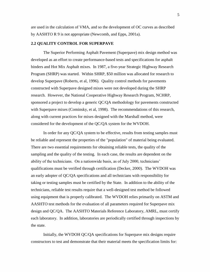
2.2 QUALITY CONTROL FOR SUPERPAVE

The Superior Performing Asphalt Pavement (Superpave) mix design method was

developed as an effort to create performance-based tests and specifications for asphalt

binders and Hot Mix Asphalt mixes. In 1987, a five-year Strategic Highway Research

Program (SHRP) was started. Within SHRP, $50 million was allocated for research to

develop Superpave (Roberts, et al, 1996). Quality control methods for pavements

constructed with Superpave designed mixes were not developed during the SHRP

research. However, the National Cooperative Highway Research Program, NCHRP,

sponsored a project to develop a generic QC/QA methodology for pavements constructed

with Superpave mixes (Cominsky, et al, 1998). The recommendations of this research,

along with current practices for mixes designed with the Marshall method, were

considered for the development of the QC/QA system for the WVDOH.

In order for any QC/QA system to be effective, results from testing samples must

be reliable and represent the properties of the "population" of material being evaluated.

There are two essential requirements for obtaining reliable tests, the quality of the

sampling and the quality of the testing. In each case, the results are dependent on the

ability of the technicians. On a nationwide basis, as of July 2000, technicians’

qualifications must be verified through certification (Decker, 2000). The WVDOH was

an early adopter of QC/QA specifications and all technicians with responsibility for

taking or testing samples must be certified by the State. In addition to the ability of the

technicians, reliable test results require that a well-designed test method be followed

using equipment that is properly calibrated. The WVDOH relies primarily on ASTM and

AASHTO test methods for the evaluation of all parameters required for Superpave mix

design and QC/QA. The AASHTO Materials Reference Laboratory, AMRL, must certify

each laboratory. In addition, laboratories are periodically certified through inspections by

the state.

Initially, the WVDOH QC/QA specifications for Superpave mix designs require

constructors to test and demonstrate that their material meets the specification limits for:

6

Asphalt Content, Pb

Voids in Total Mix, VTM

Voids in Mineral Aggregate, VMA

Voids Filled with Asphalt, VFA, and

Dust to Effective Binder, D/B.

Specification limits of the above characteristics are presented in Table 2.1 (Material

Procedure 401.02.29). All test results, with the exception of VFA, are recorded to one

tenth percent. VFA is recorded as a whole percent. The WVDOH subsequently dropped

the VFA requirement from the QC/QA specifications (Epperly, 2003).

Table 2.1: WVDOH Quality Control Mix Property Tolerances

Since these properties are dependent upon a combination of aggregates and

asphalt cement, the other factors that could change the quality of the Hot Mix Asphalt

(HMA) also need to be checked for quality control. For instance, temperature, moisture,

and fractured faces must also be checked. A complete list of the properties checked by

the WVDOH is provided in Table 2.2 (Material Procedure 401.03.50). Table 2.2 shows

the test or action being checked, the frequency with which it is checked, the standard test

method used, and the method of documenting the results.

7

Table 2.2: Guide for Quality Control Plans for Superpave Designed Hot-Mix

Asphalt

At the start of a construction project, constructors are required to verify that the

mix produced at the plant faithfully replicates the volumetric parameters from the mix

design. During verification, the constructor randomly collects a sample during each three

hours of production, with no more than three samples per day. The volumetric and

gradation parameters of the samples are evaluated and compared to the specification

criteria for the mix design. If all the samples are within the requirements, the mix

production is verified and the constructor proceeds with the construction. If the test

parameters are outside of the specification limits, production adjustments are made and

8

the constructor collects three additional samples. If the results from these samples are

acceptable, production continues. Otherwise, the constructor must halt production until

the plant or mix proportions are adjusted and verified.

Once a mix is verified, the normal QC/QA process is followed. The number of

samples required is based on the following schedule:

Production time Sampling schedule

Less than six hours One sample

More than six hours but less

than twelve hours

One sample for each half of the production period

More than twelve hours One sample for first six hour period

One sample for the second six hour period

One sample for the remaining time

All samples are tested for the volumetric parameters, asphalt content and gradation. The

results are evaluated for specification compliance based on a four-test moving average.

Control charts are maintained and made available to the WVDOH for inspection. If the

moving average of a test result, or three consecutive gradation results, falls outside of the

specification limits, the production shall be halted until the constructor takes the

necessary steps to bring the production under control. The quantity of material falling

outside of the limits is computed and a price adjustment is applied.

2.3 QUALITY ASSURANCE FOR SUPERPAVE

While the constructor has responsibility for quality control, the WVDOH has the

responsibility for verification of the quality control, or quality assurance. Three methods

are allowed in the Division's MP 401.02.29 for quality verification:

By conducting independent sampling and testing

By witnessing or reviewing the constructor's sampling and testing or

By a combination of 1 and 2.

When independent sampling and testing is conducted, the Division samples

approximately 10% of the sampling rate specified in the constructor's quality control

plan. Samples are tested in district offices by WVDOH technicians. The parameters

9

evaluated for quality assurance are the same as the quality control parameters with the

exception of the dust to binder ratio. This parameter is not evaluated during quality

assurance. The procedures for evaluating the results of the QA tests are specified in

WVDOH MP 700.00.54.

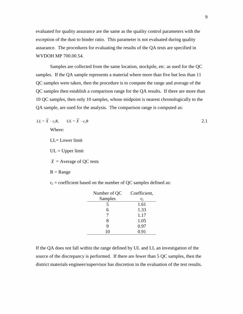
Samples are collected from the same location, stockpile, etc. as used for the QC

samples. If the QA sample represents a material where more than five but less than 11

QC samples were taken, then the procedure is to compute the range and average of the

QC samples then establish a comparison range for the QA results. If there are more than

10 QC samples, then only 10 samples, whose midpoint is nearest chronologically to the

QA sample, are used for the analysis. The comparison range is computed as:

RcXULRcXLL ii , 2.1

Where:

LL= Lower limit

UL = Upper limit

X = Average of QC tests

R = Range

ci = coefficient based on the number of QC samples defined as:

Number of QC

Samples

Coefficient,

ci

5 1.61

6 1.33

7 1.17

8 1.05

9 0.97

10 0.91

If the QA does not fall within the range defined by UL and LL an investigation of the

source of the discrepancy is performed. If there are fewer than 5 QC samples, then the

district materials engineer/supervisor has discretion in the evaluation of the test results.

10

2.4 STANDARD TEST METHODS FOR SUPERPAVE MIXES

AASHTO and ASTM provide standard-testing procedures used in the evaluation

of hot mix asphalt (HMA). Each organization publishes books stating a standard

procedure by which tests should be carried out to obtain the least variable results. These

tests may be identical in procedure and statistical variation of results, but are simply

designated by a different test number. For example, the test for Sieve Analysis of Fine

and Coarse Aggregates is designated as T 27-99 by AASHTO and C 136-96 by ASTM.

Other tests have minor differences in the method or instrumentation used, which will vary

the resulting precision and variability of the tests on the same material property test.

Table 2.3 provides a list of the volumetric quality control parameters, the

equations used to calculate the parameters and the AASHTO and ASTM tests used to

obtain the parameters. Table 2.4 provides a list of AASHTO and ASTM standard test

methods that impact the quality control parameters of a HMA once the parameters are

disaggregated to identify the individual tests and equations needed to determine the

QC/QA parameters.

In calculating the P0.075 for D/B, two methods are available. The first method

included the percent passing the 0.075 mm sieve of each stockpile being subject to a

standard deviation from AASHTO T27. This method would then add the resulting

percent passing the 0.075 mm sieve amounts and this value would be used in the D/B

calculation. The second method involved adding the percent passing each stockpile

together first. Then the standard deviation for a 500 g sample for passing the 0.075 mm

sieve was used as the standard deviation. This standard deviation can also be found in

AASHTO T27.

11

mm

mb

G

GVTM 1

Table 2.3: Volumetric Quality Control Parameters

Volumetric Parameter Equation AASHTO & ASTM Tests Required

Air Voids (VTM)

AASHTO T 166, T 209

Voids in Mineral

Aggregate

(VMA)

AASHTO T 27, T 84, T 85, T 209

ASTM D 70

Voids Filled with

Asphalt

(VFA)

AASHTO T 27, T 84, T 85, T 166, T 209

ASTM D 70

Dust to Binder Ratio b

b

mm

b

se

G

P

G

PG

100

100 b

sesb

sbse

ba PGG

GGP

)*(

)(100

s

ba

bbe PP

PP100

AASHTO T 11, T 27, T 84, T 85, T 209

ASTM D 70

VMA

VTMVMAVFA

sb

bmb

G

PGVMA

)1(1

bePBD 075.0P

/

12

Table 2.4: AASHTO and ASTM Test Methods Affecting Quality Control

Test Number Test Name

AASHTO PP-28

AASHTO TP 4

AASHTO T 11 Materials Finer Than No. 200 Sieve in Mineral Aggregates by Washing

AASHTO T 19/T 19M-00 Bulk Density and Voids in Aggregate

AASHTO T 27 Sieve Analysis of Fine and Coarse Aggregates

AASHTO T 30 Mechanical Analysis of Extracted Aggregate

AASHTO T 84 Specific Gravity and Absorption of Fine Aggregate

AASHTO T 85 Specific Gravity and Absorption of Coarse Aggregate

AASHTO T 164 Quantitative Extraction of Bituminous Paving Mixtures

AASHTO T 166 Bulk Specific Gravity of Compacted Asphalt Mixtures Using Saturated Surface-Dry Specimens

AASHTO T 195 Determining Degree of Particle Coating of Bituminous-Aggregate Mixtures

AASHTO T 209 Theoretical Maximum Specific Gravity and Density of Bituminous Paving Mixtures

AASHTO T 240 Effect of Heat and Air on a Moving Film of Asphalt (Rolling Thin Film Oven)

AASHTO T 269 Percent Air Voids in Compacted Dense and Open Bituminous Paving Mixtures

AASHTO T304 Uncompacted Void Content of Fine Aggregate

AASHTO T308 (METHOD A) Determining the Asphalt Binder Content of Hot-Mix Asphalt by Ignition Method

ASTM D70-82 Specific Gravity and Density of Semi-Solid Bituminous Materials

ASTM D5821 Determining the Percentage of Fractured Faces in Coarse Aggregate

13

2.5 PRECISION STATEMENTS

Precision statements are provided in the AASHTO and ASTM test methods used

in evaluating asphalt mixture properties. These precision statements provide either the

standard deviation or the coefficient of variation values for each test as well as an

acceptable range between results. The coefficient of variation equals the standard

deviation of a test method divided by the mean value of a set of tests, expressed in

percent. The acceptable range for the difference between two tests equals the standard

deviation or the percent coefficient of variation multiplied by 2.83 (2 2). This allowable

range is termed the two-sigma limit, d2s, when the standard deviation is provided or the

d2s in percent when the coefficient of variation is given. The two-sigma limit was

selected to provide a 95% degree of confidence when making a comparative statement

about the test results:

The d2s index is the difference between two individual test

results that would be equaled or exceeded in the long run

in only 1 case in 20 in the normal and correct operation of

the method. (ASTM, 2000)

The precision statements include values for test results for within laboratory and

between laboratory tests. The precision statement for the within laboratory is defined for

a single technician testing samples using a single set of equipment in one laboratory. The

between laboratory statement is for replicate samples tested in two different laboratories

by different technicians, using similar equipment and conditions. Tables 2.5, 2.6, and 2.7

provide information from the precision statements for each test method used for quality

control for both within and between laboratory results. Table 2.5 was compiled from the

different test methods. Tables 2.6 and 2.7 were obtained from AASHTO test method

T-27.

14

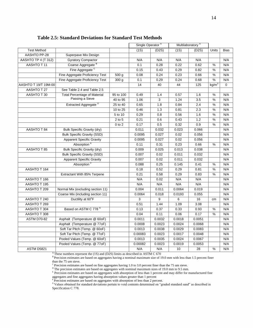
Table 2.5: Standard Deviations for Standard Test Methods

Single Operator A Multilaboratory

A

Test Method (1S) (D2S) (1S) (D2S) Units Bias

AASHTO PP-28 Superpave Mix Design

AASHTO TP 4 (T 312) Gyratory Compactor N/A N/A N/A N/A N/A

AASHTO T 11 Coarse Aggregate B 0.1 0.28 0.22 0.62 % N/A

Fine Aggregate C 0.15 0.43 0.29 0.82 % N/A

Fine Aggregate Proficiency Test 500 g 0.08 0.24 0.23 0.66 % N/A

Fine Aggregate Proficiency Test 300 g 0.1 0.29 0.24 0.68 % N/A

AASHTO T 19/T 19M-00 14 40 44 125 kg/m3 0

AASHTO T 27 See Table 2.4 and Table 2.5

AASHTO T 30 Total Percentage of Material Passing a Sieve

95 to 100 0.49 1.4 0.57 1.6 % N/A

40 to 95 1.06 3 1.24 3.5 % N/A

Extracted Aggregate D 25 to 40 0.65 1.8 0.84 2.4 % N/A

10 to 25 0.46 1.3 0.81 2.3 % N/A

5 to 10 0.29 0.8 0.56 1.6 % N/A

2 to 5 0.21 0.6 0.43 1.2 % N/A

0 to 2 0.17 0.5 0.32 0.9 % N/A

AASHTO T 84 Bulk Specific Gravity (dry) 0.011 0.032 0.023 0.066 N/A

Bulk Specific Gravity (SSD) 0.0095 0.027 0.02 0.056 N/A

Apparent Specific Gravity 0.0095 0.027 0.02 0.056 N/A

Absorption E 0.11 0.31 0.23 0.66 % N/A

AASHTO T 85 Bulk Specific Gravity (dry) 0.009 0.025 0.013 0.038 N/A

Bulk Specific Gravity (SSD) 0.007 0.02 0.011 0.032 N/A

Apparent Specific Gravity 0.007 0.02 0.011 0.032 N/A

Absorption F 0.088 0.25 0.145 0.41 % N/A

AASHTO T 164 0.18 0.52 0.29 0.81 % N/A

Extractant With 85% Terpene 0.21 0.58 0.29 0.83 % N/A

AASHTO T 166 N/A 0.02 N/A N/A N/A

AASHTO T 195 N/A N/A N/A N/A N/A

AASHTO T 209 Normal Mix (excluding section 11) 0.004 0.011 0.0064 0.019 N/A

Coarse Mix (including section 11) 0.0064 0.018 0.0193 0.055 N/A

AASHTO T 240 Ductility at 60oF 3 9 6 16 cm N/A

AASHTO T 269 0.51 1.44 1.09 3.08 N/A

AASHTO T 304 Based on ASTM C 778 G 0.13 0.37 0.33 0.93 % N/A

AASHTO T 308 0.04 0.11 0.06 0.17 % N/A

ASTM D70-82 Asphalt (Temperature @ 60oF) 0.0011 0.0032 0.0018 0.0051 N/A

Asphalt (Temperature @ 77oF) 0.0008 0.0023 0.0024 0.0068 N/A

Soft Tar Pitch (Temp. @ 60oF) 0.0013 0.0038 0.0029 0.0083 N/A

Soft Tar Pitch (Temp. @ 77oF) 0.00083 0.0023 0.0017 0.0048 N/A

Pooled Values (Temp. @ 60oF) 0.0013 0.0035 0.0024 0.0067 N/A

Pooled Values (Temp. @ 77oF) 0.00082 0.0023 0.0019 0.0053 N/A

ASTM D5821 N/A N/A 10 28 % N/A A These numbers represent the (1S) and (D2S) limits as described in ASTM C 670 B Precision estimates are based on aggregates having a nominal maximum size of 19.0 mm with less than 1.5 percent finer

than the 75 um sieve. C Precision estimates are based on fine aggregates having 1.0 to 3.0 percent finer than the 75 um sieve. D The precision estimates are based on aggregates with nominal maximum sizes of 19.0 mm to 9.5 mm. E Precision estimates are based on aggregates with absorption of less than 1 percent and may differ for manufactured fine

aggregates and fine aggregates having absorption values greater than 1 percent F Precision estimates are based on aggregates with absorption of less than 2 percent. G Values obtained for standard deviations pertain to void contents determined on “graded standard sand” as described in

Specification C 778.

15

Table 2.6: Standard Deviations for AASHTO T-27

Total

Percent of

Material

Passing

Single Operator A Multilaboratory A

(1S) (D2S) (1S) (D2S)

Coarse

AggregateB

95 to 100 0.32 0.9 0.35 1

85 to 95 0.81 2.3 1.37 3.9

80 to 85 1.34 3.8 1.92 5.4

60 to 80 2.25 6.4 2.82 8

20 to 60 1.32 3.7 1.97 5.6

15 to 20 0.95 2.7 1.6 4.5

10 to 15 1 2.8 1.43 4.2

5 to 10 0.75 2.1 1.22 3.4

2 to 5 0.53 1.5 1.04 3

0 to 2 0.27 0.8 0.45 1.3

Fine

Aggregate

95 to 100 0.25 0.7 0.23 0.6

60 to 95 0.55 1.6 0.77 2.2

20 to 60 0.83 2.4 1.41 4

15 to 20 0.54 1.5 1.1 3.1

10 to 15 0.36 1 0.73 2.1

2 to 10 0.37 1.1 0.65 1.8

0 to 2 0.14 0.4 0.31 0.9

A These numbers represent, respectively, the (1sS) and (d2s) limits as described in

ASTM C 670

B The precision estimates are based on aggregates with nominal maximum size of

19.0 mm.

16

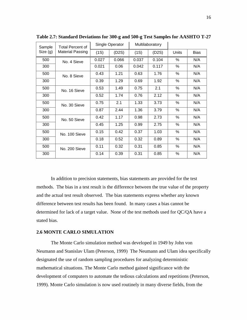
Table 2.7: Standard Deviations for 300-g and 500-g Test Samples for AASHTO T-27

Sample Size (g)

Total Percent of Material Passing

Single Operator Multilaboratory

(1S) (D2S) (1S) (D2S) Units Bias

500 No. 4 Sieve

0.027 0.066 0.037 0.104 % N/A

300 0.021 0.06 0.042 0.117 % N/A

500 No. 8 Sieve

0.43 1.21 0.63 1.76 % N/A

300 0.39 1.29 0.69 1.92 % N/A

500 No. 16 Sieve

0.53 1.49 0.75 2.1 % N/A

300 0.52 1.74 0.76 2.12 % N/A

500 No. 30 Sieve

0.75 2.1 1.33 3.73 % N/A

300 0.87 2.44 1.36 3.79 % N/A

500 No. 50 Sieve

0.42 1.17 0.98 2.73 % N/A

300 0.45 1.25 0.99 2.75 % N/A

500 No. 100 Sieve

0.15 0.42 0.37 1.03 % N/A

300 0.18 0.52 0.32 0.89 % N/A

500 No. 200 Sieve

0.11 0.32 0.31 0.85 % N/A

300 0.14 0.39 0.31 0.85 % N/A

In addition to precision statements, bias statements are provided for the test

methods. The bias in a test result is the difference between the true value of the property

and the actual test result observed. The bias statements express whether any known

difference between test results has been found. In many cases a bias cannot be

determined for lack of a target value. None of the test methods used for QC/QA have a

stated bias.

2.6 MONTE CARLO SIMULATION

The Monte Carlo simulation method was developed in 1949 by John von

Neumann and Stanislav Ulam (Peterson, 1999) The Neumann and Ulam idea specifically

designated the use of random sampling procedures for analyzing deterministic

mathematical situations. The Monte Carlo method gained significance with the

development of computers to automate the tedious calculations and repetitions (Peterson,

1999). Monte Carlo simulation is now used routinely in many diverse fields, from the

17

simulation of complex physical phenomena such as radiation transport in the earth's

atmosphere to the simulation of a Bingo game (USDOE, 2003). The simulation process

allows the user to include the inherent uncertainty associated with each input parameter

into the analysis. The output of a Monte Carlo simulation is a probability distribution

describing the probability associated with each possible outcome.

The major components of a Monte Carlo simulation include the following:

Probability distribution functions (pdf's) - the physical (or mathematical) system

must be described by a set of pdf's.

Random number generator - a source of random numbers uniformly distributed

on the unit interval must be available.

Sampling rule - a prescription for sampling from the specified pdf's, assuming the

availability of random numbers on the unit interval, must be given.

Scoring (or tallying) - the outcomes must be accumulated into overall tallies or

scores for the quantities of interest.

Error estimation - an estimate of the statistical error (variance) as a function of

the number of trials and other quantities must be determined.

Variance reduction techniques - methods for reducing the variance in the

estimated solution to reduce the computational time for Monte Carlo simulation

Parallelization and vectorization - algorithms to allow Monte Carlo methods to

be implemented efficiently on advanced computer architectures. (USDOE, 2003)

Figure 2.1 illustrates a general schematic for a Monte Carlo simulation

(Hutchinson and Bandalos, 1997). The first step of a Monte Carlo simulation is to

identify a deterministic model where multiple input variables are used to estimate a single

value outcome. The next step requires that all variables or parameters be identified.

Then, the type of probability distribution for each independent variable is established for

the simulation model, (e.g. normal, beta, log normal, etc). Next, a random trial process is

initiated to establish a probability distribution function for the deterministic situation

being modeled. During each pass, a random value from the distribution function for each

parameter is selected and used into the calculation. Multiple solutions are obtained by

making a large number of passes through the program obtaining a solution for each pass.

The appropriate number of passes for an analysis is a function of the number of input

parameters, the complexity of the modeled situation, and the desired precision of the

18

output. The final result of a Monte Carlo simulation is a probability distribution of the

output parameter (Peterson, 1999).

Trials

N Times

Monte

Carlo

Simulation

PDF for Deterministic Situation

Probability Distribution Function

Established

Random Trial of Parameters

for Deterministic Situation

Distribution Analysis

Independent Parameters or Variables

Deterministic Situation

Figure 2.1: General Monte Carlo Simulation Approach

The Monte Carlo method requires numerous repetitive calculations and sampling

of the distribution of the independent variables in the analysis. Even with modern

computers, it is tedious to program a Monte Carlo simulation procedure. However,

commercial tools are available to reduce the burden on the analysis for developing a

Monte Carlo simulation. The @Risk software is an add-in extension for Microsoft's

Excel (Palisade Corporation, 1997). @Risk allows the user to select from a variety of

distributions, perform the simulation, and then display the results of the simulation.

@Risk has been successfully used at WVU for the simulation of slope stability and

evaluation of preventive maintenance strategies (Peterson, 1999 and Reigle, 2000)

One of the advantages of using the @Risk software is the ability to readily define

the type of distribution and sampling method used for the MCS. The Latin Hypercubic

sampling procedure, available in @Risk is designed to accurately recreate an input

distribution through sampling in fewer iterations by stratification of the input probability

distributions. Stratification divides a probability distribution cumulative curve into equal

intervals on the cumulative probability scale (0 to 1.0) from each interval or

“stratification” of the input distribution (Palisade Corporation, 1997). The simulation

19

begins with a randomly selected sample or value for each of the independent variables

and the deterministic equations are exercised to compute independent variables in the

analysis. A new set of values for the independent variables is established for the next

step in the simulation. The simulation continues until the termination criteria are met.

@Risk allows termination of the simulation when either a fixed number of iterations are

completed or when the mean and standard deviations changed by less than a user-

specified amount. In the latter case, changes in the mean and standard deviations are

tested after a user specified number of iterations.

Hand and Epps (2000) used Monte Carlo Simulation to assess the effects of

variability in materials and mixture property measurements on volumetric properties and

optimum asphalt content selection for the mix design of hot mix asphalt. Superpave and

Marshall volumetric parameters were considered in this paper. The volumetric

parameters of interest were VTM, VMA, VFA, percent compaction at initial (%Gmm,ini)

and maximum (%Gmm,max) number of gyrations, and the dust to binder ratio. In order to

calculate the volumetric parameters, the following properties were required:

Asphalt content (AC)

Combined aggregate bulk specific gravity (Gsb)

Asphalt cement specific gravity (Gb)

Bulk specific gravity of compacted specimens (Gmb)

Theoretical maximum specific gravity of the mix (Gmm)

The amount of material passing the 0.075 mm sieve (P0.075mm)

The values of AC and P0.075mm are controlled in the laboratory for mix designs.

The other properties are found experimentally. Therefore each property, Gb, Gsb, Gmb,

and Gmm, have variability associated with its test method. Both AASHTO and ASTM

test methods were researched to obtain precision statements. The Gsb, used in volumetric

calculations, is the weighted average of the coarse and fine aggregate Gsb values and thus

has two individual standardized tests. The standard deviation for this property was also a

weighted average of the standard deviations of the Gsb test for coarse and fine aggregates.

All other standard deviations are found from one test method.

20

The Monte Carlo Simulation was run using convergence of three parameters as

the basis for the number of iterations performed. The standard deviation, mean, and

percentiles (0 percent to 100 percent in 5 percent increments) for each output parameter

were used as the convergence parameters. The convergence threshold of 0.75 percent was

used for the termination point of the simulation. The simulation was evaluated every 100

iterations to check for the convergence threshold. The simulation was run using both

within laboratory precision and between laboratory precisions. The results were then

tabulated and discussed.

The results of the simulation presented the following distribution statistics for

each volumetric property:

Standard deviation

Minimum observation

Maximum observation

Volumetric property values at plus and minus one standard deviation from

the mean (+1 Std Dev and -1 Std Dev)

Volumetric property values at plus and minus two standard deviation from

the mean (+2 Std Dev and -2 Std Dev)

5th

, 10th

, 25th

, 50th

, 75th

, 90th

, and 95th

percentiles.

Through the Monte Carlo simulation Hand and Epps (2000) demonstrated there

was "tremendous" variability in the expected volumetric and mix design parameters as a

result of the level of precision afforded by the testing methods. This research

demonstrated that for a Superpave mix design where the optimum asphalt content for the

"average" condition was 5.75 percent, the range in asphalt contents that is embraced

within the 5 to 95 percentiles is 5.33 to more than 6.75 percent. This analysis was based

on within lab variability. Larger ranges of results were obtained when the between lab

precision statements were considered. Hand and Epps (2000) concluded:

The effects of what is currently considered acceptable test

variability on volumetrics and AC selection are unacceptable in

light of the new types of specifications being implemented. These

specifications place mix design responsibility on the contractor and

21

mix design verification responsibility with the owner or agency.

Verifying agencies are going to have to recognize the fact that

variability exists and has a large potential impact to result in

differences in mix design. This statement is also true for field

management operations. This will ultimately drive the

development of much needed mix design verification criteria and

specifications.

2.7 SUMMARY

The specifications used by WVDOH represent the state-of-the-practice method

for specifying and controlling the quality of HMA construction. While the design of the

end product specification method is sound, the ability of these specifications is dependent

on the precision of the test methods used to measure the control parameters. AASHTO

and ASTM both include precision statements in all test methods used for HMA

construction quality control and acceptance. Some of the parameters used for quality

control and assurance are derived through a combination of test procedures making the

determination of the variability of the parameter problematic. Monte Carlo simulation

provides a technique for determining the overall variability of a process when that

process is the result of several individual processes, each with its own variability. Hand

and Epps (2000) performed a Monte Carlo simulation of the Marshall and Superpave mix

design processes and concluded that the lack of precision in test methods and

subsequently mix design parameters was unacceptable. They speculated that "field

management", i.e. QC/QA, also suffers from a lack of precision in the testing method, but

did not perform research to support this statement.

22

CHAPTER 3 RESEARCH METHODOLOGY

3.1 INTRODUCTION

The literature review established the QC/QA method used by WVDOH, required

test methods, and the fact that there are potential problems with the risks associated with

the purchase decisions. The risk lies in accepting an unacceptable mix or accepting a

substandard mix. Monte Carlo simulation was identified as a tool that could assist with

determining the distribution of the QC/QA parameters as a function of the testing

protocol with appropriate consideration of the variability of the test methods. The

methodology was exercised for several mix designs that are typical of those constructed

in West Virginia.

3.2 RESEARCH APPROACH

The evaluation of the QC/QA process involved several steps:

1. Review the WVDOH QC/QA methods

2. Identify QC/QA parameters

3. Identify tests required to quantify QC/QA parameters

4. Determine test method variability from the precision statement for each test

method

5. Identify equations for computing QC/QA parameters from test results

6. Select method to quantify total variability in QC/QA parameter when multiple

test methods are required.

7. Develop and verify models for quantifying parameter variability.

8. Exercise models for multiple mix types typically used by WVDOH.

9. Interpret results.

The first four steps of this research approach were accomplished during the

literature review as presented in Chapter 2. The equations needed for the analysis were

also identified during the literature review. However, the structure for implementing

23

these equations to determine the PDF for the QC/QA parameters is more explicitly set

forth in the following.

Monte Carlo simulation was used for the sixth step in the procedure. Palisade's

@Risk add-in program for Excel was used for the quality control analysis. However, for

the quality assurance analysis, additional parameter testing was required in a manner that

is not convenient to capture in an @Risk analysis. Therefore, a Visual Basic for

Applications, VBA, program was developed to execute the quality assurance analysis.

Exercising the models over simple data sets where the output could be predetermined

validated both the @Risk and VBA models.

Once the Monte Carlo models were developed and the associated variability of

the test methods was identified, the models were exercised over a range of mix types used

throughout the state. It was necessary to evaluate different mixes because:

The mean values of the mix design parameters change, establishing different

acceptance ranges,

Some of the precision statements are expressed in percent coefficient of variation.

In these cases, the variability of the test increases as the mean value for the

test changes, and

The WVDOH quality control parameters are a function of the nominal maximum

aggregate size for the mix.

The experiment was run using three mix designs of different classifications. The first mix

design was a 37.5 mm Superpave mix followed by a 19 mm mix and a 9.5 mm mix. The

basic procedure used to test each mix type was similar; however, each mix type had

different values for each property that had to be taken into consideration. To

accommodate the changing variable values, a master file for using the @Risk software

and Excel was first created. The @Risk software is the program that ran the Monte Carlo

simulations for each of the test parameters that affects quality control.

3.3 QUALITY CONTROL MODEL

Figure 3.1 shows how the Monte Carlo structure of Figure 2.1 was applied to this

research. The MCS was applied to several mixes used in West Virginia, varying the

24

nominal maximum aggregate size and the type of binder, as summarized in Table 3.1.

First, the volumetric parameters evaluated during the analysis, and their associated

equations are defined. These are represented as yk in Figure 3.1. The equations used in

the MCS are presented in Table 2.3. This allows identification of the independent

variables, represented as xj in Figure 3.1. For this analysis, four dependent variables used

for quality control were evaluated, i.e. xj represents VTM, VMA, VFA, and D/B from

Table 2.3. VMA and D/B are dependent on the bulk specific gravity of the aggregate,

Gsb. The calculation of Gsb is somewhat convoluted so the discussion of this parameter is

deferred to a later section.

Table 3.1: Mix Design Types Evaluated with MCS

Binder Type

NMAS* PG 64-22 PG 70-22 PG 76-22

9.5 mm X X

12.5 mm X

19 mm X X

37.5 mm X X

* Nominal Maximum Aggregate Size

In a deterministic analysis, a single value, typically the mean, is assigned to each

independent variable. For this analysis, mean values from WVDOH T400 mix design

sheets were used for each of the independent variables. Next, the parameter defining the

distribution of each independent variable is determined. For this analysis, it was assumed

by AASHTO and ASTM that all independent variables have a normal distribution, so

their probability distribution function is completely defined by the mean and standard

deviation. The standard deviation for each independent variable is defined as j on

Figure 3.1 and is equal to the standard deviation determined from the precision statement

for each test method. During the quality control process, constructor personnel perform

all the testing in the constructor's laboratory. It was assumed that the precision statement

for the within laboratory test condition applies to this situation. Note VFA is computed

from VTM and VMA; this calculation was performed for each iteration during the

simulation to determine the PDF for VFA.

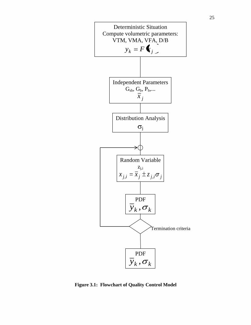
25

Figure 3.1: Flowchart of Quality Control Model

Distribution Analysis

j

Random Variable

zj,i

jijjij zxx ,,

PDF

kky ,

Termination criteria

PDF

kky ,

Deterministic Situation

Compute volumetric parameters:

VTM, VMA, VFA, D/B

jk xFy

Independent Parameters

Gsb, Gb, Pb,...

jx

26

With the equations and dependent variables defined, the Monte Carlo simulation

was performed. Within @Risk, a random variable was generated and used to "sample"

the distribution for each of the independent variables and the deterministic equations are

evaluated to determine a value for each dependent variable. For this analysis, a Latin

Hypercubic sampling method was used. The statistics for the probability distribution

function of the dependent variables are accumulated for each step in the simulation,

followed by evaluation of the termination criteria. The simulation is terminated when the

termination criteria are met. For this analysis, the simulation was terminated when there

was less than a 0.75 percent difference between the means or standard deviations

computed in increments of 100 simulation steps or when 10,000 simulation steps were

completed.

The asphalt content of a mix, expressed as percent binder, Pb, is a quality control

parameter. Pb is measured directly using the ignition oven method, AASHTO T308.

Since the expected value is known from the mix design and the standard deviation is

known from the test method, it is not necessary or meaningful to determine the

distribution of this parameter with MCS.

As shown on Figure 3.1, the output from the MCS is a probability distribution

function for each of the dependent variables. Since the independent variables were

normally distributed, all relationships in the simulation are linear functions, the resulting

PDF is also normally distributed (Differences, 2005) . Hence, the output probability

distribution is completely defined by the mean and standard deviation.

3.3.1 Standard Deviation of Sample of Means

In performing the simulation, each iteration is a simulation of an individual test.

The WVDOH QC/QA procedures are based on averaging four consecutive tests to

determine the percent of the material that is within limits. In order to use the output from

the MCS for evaluation of the WVDOH QC/QA specifications, it is necessary to adjust

the standard deviation. The standard deviation of a sample of means is computed as

(Cominsky, et al., 1998):

nx , 3.1

27

Where:

x = standard deviation of sample means of sample size n

= standard deviation

n = number of samples averaged to obtain one result (n = 4; for WVDOH QC)

This equation resulted in all the standard deviations being divided by the square

root of four, or simply dividing by two. The resulting value is termed the standard

deviation of sample means.

3.3.2 Percent Within Limits

Once the PDF for each quality control parameter was determined from the MCS,

the percent of test results either within or outside of the WVDOH control limits was

calculated. The control limits are established using the parameters in Table 2.1. The Z

value is a statistical value denoting the number of standard deviations that the upper or

lower limits are from the mean value. The Z value was calculated as (Darlington and

Carlson, 1975):

x

xCLZ 3.2

Where:

CL = control limit, may be upper or lower control limit

x = mean

x = standard deviation of sample means

This equation used the WVDOH upper and lower control limits for QC and the

mean and standard deviation of means to establish two Z values. One value represents the

upper limit and the other represents the lower limit. The Excel function

NORMSDIST(Z) was used to determine the percent outside the limit for a one -tailed

test. The percent outside the limit is then subtracted from 100 to obtain the percent

within either the upper or lower limits.

28

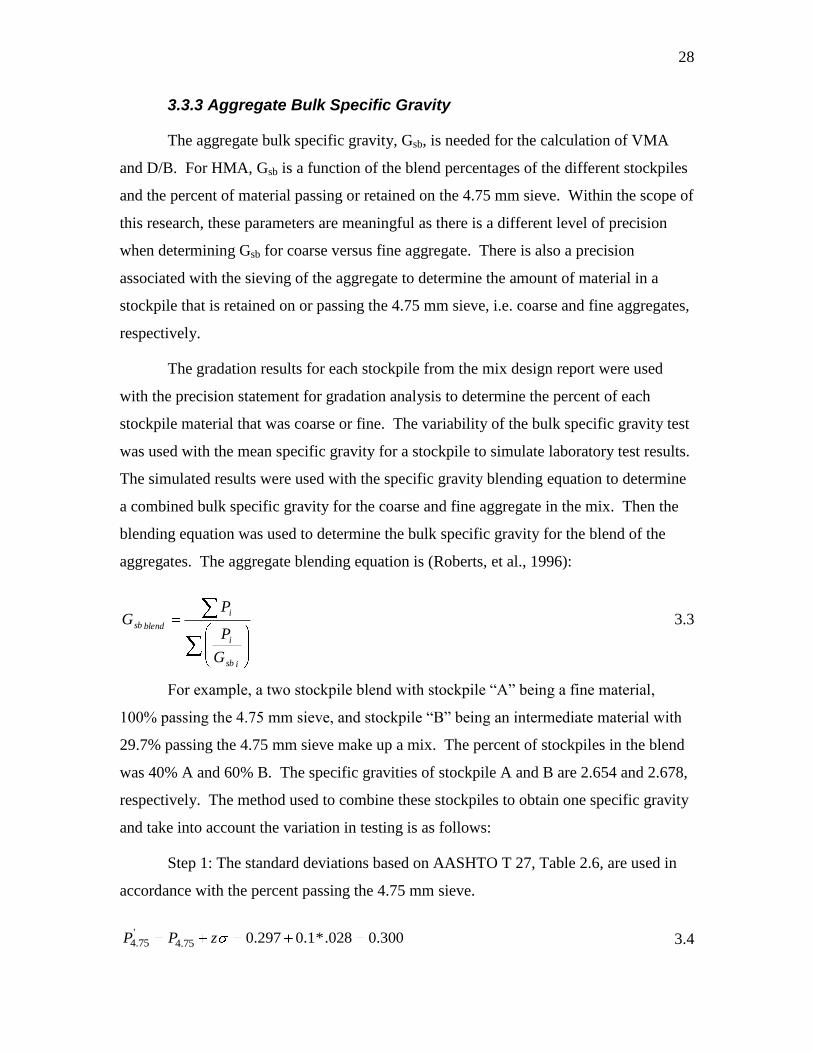
3.3.3 Aggregate Bulk Specific Gravity

The aggregate bulk specific gravity, Gsb, is needed for the calculation of VMA

and D/B. For HMA, Gsb is a function of the blend percentages of the different stockpiles

and the percent of material passing or retained on the 4.75 mm sieve. Within the scope of

this research, these parameters are meaningful as there is a different level of precision

when determining Gsb for coarse versus fine aggregate. There is also a precision

associated with the sieving of the aggregate to determine the amount of material in a

stockpile that is retained on or passing the 4.75 mm sieve, i.e. coarse and fine aggregates,

respectively.

The gradation results for each stockpile from the mix design report were used

with the precision statement for gradation analysis to determine the percent of each

stockpile material that was coarse or fine. The variability of the bulk specific gravity test

was used with the mean specific gravity for a stockpile to simulate laboratory test results.

The simulated results were used with the specific gravity blending equation to determine

a combined bulk specific gravity for the coarse and fine aggregate in the mix. Then the

blending equation was used to determine the bulk specific gravity for the blend of the

aggregates. The aggregate blending equation is (Roberts, et al., 1996):

isb

i

i

blendsb

G

P

PG 3.3

For example, a two stockpile blend with stockpile “A” being a fine material,

100% passing the 4.75 mm sieve, and stockpile “B” being an intermediate material with

29.7% passing the 4.75 mm sieve make up a mix. The percent of stockpiles in the blend

was 40% A and 60% B. The specific gravities of stockpile A and B are 2.654 and 2.678,

respectively. The method used to combine these stockpiles to obtain one specific gravity

and take into account the variation in testing is as follows:

Step 1: The standard deviations based on AASHTO T 27, Table 2.6, are used in

accordance with the percent passing the 4.75 mm sieve.

300.0028.*1.0297.075.4'75.4 zPP 3.4

29

At this point, the coarse and fine specific gravity values are subject to standard

deviation based on AASHTO tests T85 and T84, respectively. These standard deviations

are found in Table 2.5. A calculated specific gravity for both coarse and fine aggregate

from each stockpile are found and used in the blend equation along with the calculated

P4.75 mm value.

Coarse Fine

678.2

678.2

7.0*60

7.0*60blendsbG 661.2

654.2

1*40

678.2

3.0*60

1*403.0*60blendsbG

Step 2: The blend equation is completed a second time to blend the coarse and

fine aggregate specific gravity values. The example calculation is:

Blend

668.2

661.2

58

678.2

42

5842blendsbG

This blend specific gravity is the specific gravity used in the VMA equation and

in calculating D/B. The value for the bulk specific gravity of the stone varies for each

iteration of the simulation since it is based on standard deviations of the gradation and

specific gravity tests.

The above procedure for considering the variation in gradation was also used to

adjust the percent material passing the 0.075 mm sieve for the dust to binder ratio

calculations. The adjusted bulk specific gravity is also used in determining the percent

binder absorbed.

3.3.4 Effects of Varying Asphalt Content

The target asphalt content suggested by the results of the mix design is sometimes

adjusted during plant production. The percent binder has an allowable range of plus or

minus 0.4 percent from the accepted job mix formula, JMF. The addition or deduction of

binder to a mix affects the volumetric parameters tested during quality control. By

varying the percent binder in increments of tenths of a percent throughout the accepted

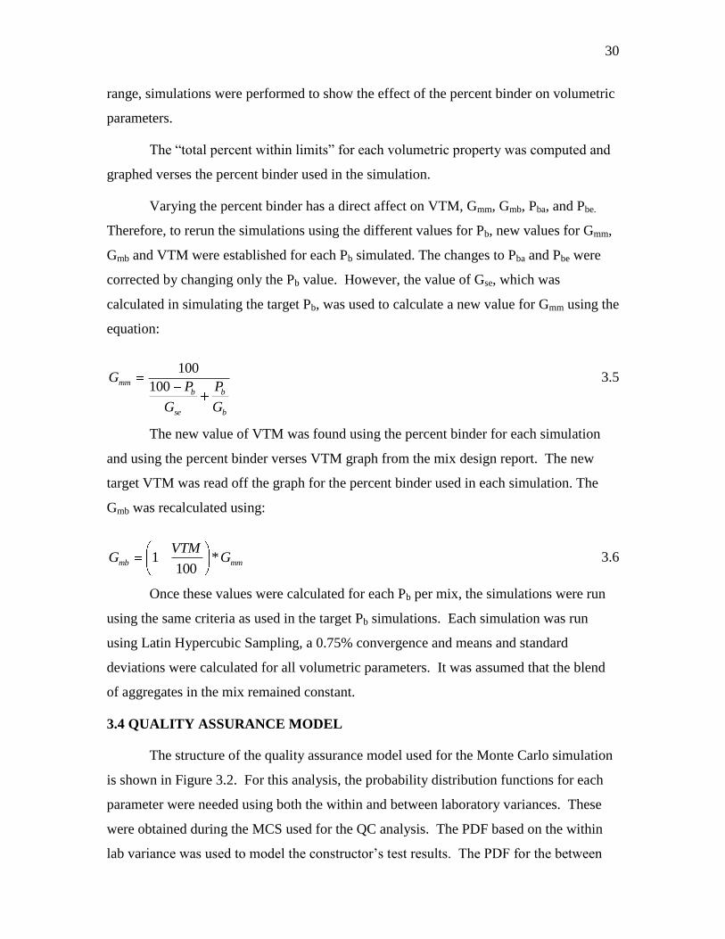
30

range, simulations were performed to show the effect of the percent binder on volumetric

parameters.

The “total percent within limits” for each volumetric property was computed and

graphed verses the percent binder used in the simulation.

Varying the percent binder has a direct affect on VTM, Gmm, Gmb, Pba, and Pbe.

Therefore, to rerun the simulations using the different values for Pb, new values for Gmm,

Gmb and VTM were established for each Pb simulated. The changes to Pba and Pbe were

corrected by changing only the Pb value. However, the value of Gse, which was

calculated in simulating the target Pb, was used to calculate a new value for Gmm using the

equation:

b

b

se

bmm

G

P

G

PG

100

100 3.5

The new value of VTM was found using the percent binder for each simulation

and using the percent binder verses VTM graph from the mix design report. The new

target VTM was read off the graph for the percent binder used in each simulation. The

Gmb was recalculated using:

mmmb GVTM

G *100

1 3.6

Once these values were calculated for each Pb per mix, the simulations were run

using the same criteria as used in the target Pb simulations. Each simulation was run

using Latin Hypercubic Sampling, a 0.75% convergence and means and standard

deviations were calculated for all volumetric parameters. It was assumed that the blend

of aggregates in the mix remained constant.

3.4 QUALITY ASSURANCE MODEL

The structure of the quality assurance model used for the Monte Carlo simulation

is shown in Figure 3.2. For this analysis, the probability distribution functions for each

parameter were needed using both the within and between laboratory variances. These

were obtained during the MCS used for the QC analysis. The PDF based on the within

lab variance was used to model the constructor’s test results. The PDF for the between

31

lab results were used to model the QA results of the WVDOH, due to the fact that the QA

tests are performed by a different technician in a different lab.

The quality assurance procedure requires that the WVDOH collect and test

independent samples to compare to the quality control results obtained by the constructor.

Generally, the WVDOH tests one sample for each 10 samples tested by the constructor,

but in some situations, a QA sample may be obtained for as few as 5 samples. Thus, the

MCS was set up to simulate the effect of varying the number of constructor samples from

5 to 10 used in comparison to the QA sample. Following the requirements of Materials

Procedure 700.00.54, the mean and range of QC test results were determined and the

allowable range for the QA results was determined using the factors presented in Chapter

2. The results of the QA test were then simulated using the PDF for between

laboratories. The simulated QA result was compared to the allowable range. If the QA

result was outside the allowable range, a counter was incremented. This process was

repeated for 1000 iterations and the percent of times the QA results was outside the

allowable range was determined for each QC parameter. The simulation was repeated for

each mix type evaluated during the QC analysis.

Due to the nature of the QA analysis, it was more convenient to write a simple

Visual Basic for Applications program to perform this simulation rather than using

@Risk. The code for this program is presented in Appendix 2.

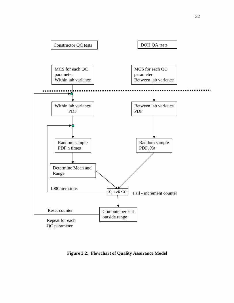
32

Figure 3.2: Flowchart of Quality Assurance Model

Constructor QC tests DOH QA tests

MCS for each QC

parameter

Within lab variance

MCS for each QC

parameter

Between lab variance

Within lab variance

PDF

Between lab variance

PDF

Random sample

PDF n times

Random sample

PDF, Xa

Determine Mean and

Range

Fail - increment counter ac XcRX :1000 iterations

Compute percent

outside range

Reset counter

Repeat for each

QC parameter

33

CHAPTER 4 METHODOLOGY APPLICATION AND RESULTS

4.1 INTRODUCTION

The methodology presented in Chapter 3 was completed using 7 mix designs for

both within laboratory and between laboratory situations. The mix designs were

composed of different gradations and different asphalt binder grades. The various

gradations were 9.5 mm, 12.5 mm, 19 mm, and 37.5 mm. The various asphalt binders

consisted of PG 64-22, PG 70-22, and PG 76-22. The seven mix designs that were

simulated can be found in Table 3.1. The probability distribution function of each

volumetric quality control parameter was evaluated and compared based on the current

WVDOH quality control specifications.

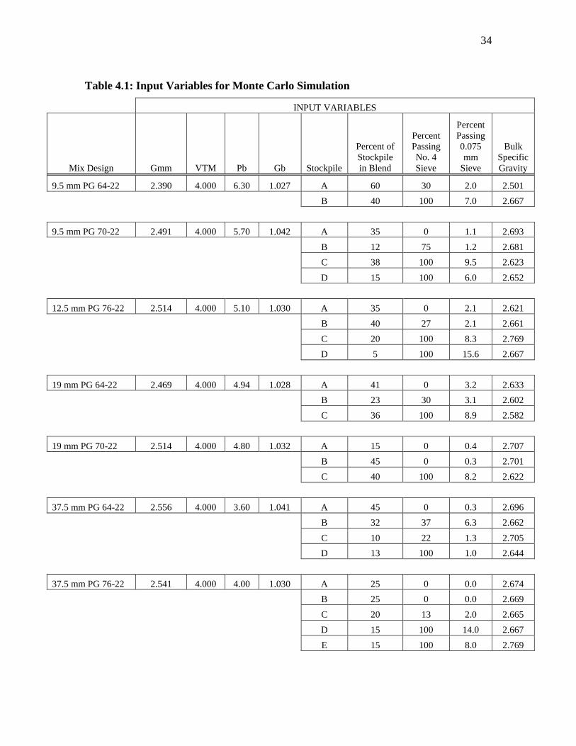
4.2 MIX DESIGN INPUT AND OUTPUT VALUES

To simulate each mix design, a number of input values must be entered in the

spreadsheet for calculations. These inputs, which are discussed in Chapter 3, vary from

one mix design to another. A summary of the required inputs and the values used for the

input variables in each mix design can be found in Table 4.1. The input variables are used

in the simulation to calculate the output variables specified by the user.

The outputs of interest for volumetric specifications are percent binder, VTM,

VMA, VFA, and Dust to Binder Ratio (D/B). The needed statistical outputs for each

volumetric parameter included the mean and the standard deviation calculated during the

simulation. The mean and standard deviation values obtained for each output variable for

each mix design can be found in Table 4.2 and Table 4.3 for the within and between

laboratory variations, respectively. The within variations were used for the evaluation of

the Quality Control parameters and the between variations were used to simulate the

Quality Assurance analysis.

34

Table 4.1: Input Variables for Monte Carlo Simulation

INPUT VARIABLES

Mix Design Gmm VTM Pb Gb Stockpile

Percent of

Stockpile

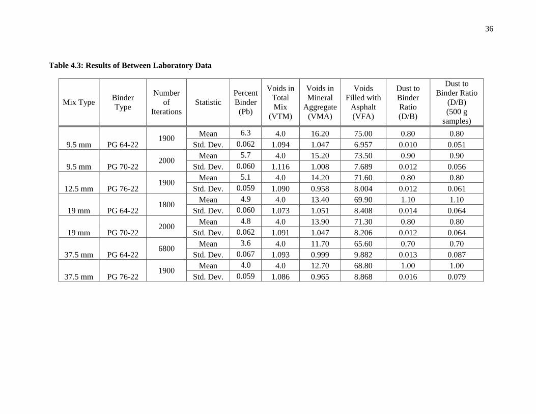
in Blend

Percent

Passing

No. 4

Sieve

Percent

Passing

0.075

mm

Sieve

Bulk

Specific

Gravity

9.5 mm PG 64-22 2.390 4.000 6.30 1.027 A 60 30 2.0 2.501

B 40 100 7.0 2.667

9.5 mm PG 70-22 2.491 4.000 5.70 1.042 A 35 0 1.1 2.693

B 12 75 1.2 2.681

C 38 100 9.5 2.623

D 15 100 6.0 2.652

12.5 mm PG 76-22 2.514 4.000 5.10 1.030 A 35 0 2.1 2.621

B 40 27 2.1 2.661

C 20 100 8.3 2.769

D 5 100 15.6 2.667

19 mm PG 64-22 2.469 4.000 4.94 1.028 A 41 0 3.2 2.633

B 23 30 3.1 2.602

C 36 100 8.9 2.582

19 mm PG 70-22 2.514 4.000 4.80 1.032 A 15 0 0.4 2.707

B 45 0 0.3 2.701

C 40 100 8.2 2.622

37.5 mm PG 64-22 2.556 4.000 3.60 1.041 A 45 0 0.3 2.696

B 32 37 6.3 2.662

C 10 22 1.3 2.705

D 13 100 1.0 2.644

37.5 mm PG 76-22 2.541 4.000 4.00 1.030 A 25 0 0.0 2.674

B 25 0 0.0 2.669

C 20 13 2.0 2.665

D 15 100 14.0 2.667

E 15 100 8.0 2.769

35

Table 4.2: Results of Within Laboratory Data

* Standard Deviation of Means

Mix Type Binder

Type

Number

of

Iterations

Statistic

Percent

Binder

(Pb)

Voids in

Total

Mix

(VTM)

Voids in

Mineral

Aggregate

(VMA)

Voids

Filled with

Asphalt

(VFA)

Dust to

Binder

Ratio

(D/B)

Dust to Binder

Ratio (D/B)

(500 g samples)

9.5 mm PG 64-22 1900

Mean 6.3 4.0 16.20 75.30 0.80 0.80

Std. Dev.* 0.021 0.259 0.250 1.631 0.004 0.010

9.5 mm PG 70-22 2000

Mean 5.7 4.0 15.20 73.50 0.90 0.90

Std. Dev.* 0.020 0.256 0.240 1.742 0.005 0.011

12.5 mm PG 76-22 1900

Mean 5.1 4.0 14.10 71.80 0.80 0.80

Std. Dev.* 0.020 0.252 0.231 1.844 0.005 0.012

19 mm PG 64-22 1800

Mean 4.9 4.0 13.50 70.20 1.10 1.10

Std. Dev.* 0.020 0.257 0.248 1.996 0.005 0.013

19 mm PG 70-22 2000

Mean 4.8 4.0 13.90 71.30 0.80 0.80

Std. Dev.* 0.020 0.263 0.242 1.973 0.004 0.013

37.5 mm PG 64-22 6800

Mean 3.6 4.0 11.70 65.80 0.70 0.70

Std. Dev.* 0.023 0.254 0.239 2.292 0.005 0.016

37.5 mm PG 76-22 1900

Mean 4.0 4.0 12.70 68.60 1.00 1.00

Std. Dev.* 0.021 0.250 0.235 2.072 0.005 0.015

36

Table 4.3: Results of Between Laboratory Data

Mix Type Binder

Type

Number

of

Iterations

Statistic

Percent

Binder

(Pb)

Voids in

Total

Mix

(VTM)

Voids in

Mineral

Aggregate

(VMA)

Voids

Filled with

Asphalt

(VFA)

Dust to

Binder

Ratio

(D/B)

Dust to

Binder Ratio

(D/B)

(500 g

samples)

9.5 mm PG 64-22 1900

Mean 6.3 4.0 16.20 75.00 0.80 0.80

Std. Dev. 0.062 1.094 1.047 6.957 0.010 0.051

9.5 mm PG 70-22 2000

Mean 5.7 4.0 15.20 73.50 0.90 0.90

Std. Dev. 0.060 1.116 1.008 7.689 0.012 0.056

12.5 mm PG 76-22 1900

Mean 5.1 4.0 14.20 71.60 0.80 0.80

Std. Dev. 0.059 1.090 0.958 8.004 0.012 0.061

19 mm PG 64-22 1800

Mean 4.9 4.0 13.40 69.90 1.10 1.10

Std. Dev. 0.060 1.073 1.051 8.408 0.014 0.064

19 mm PG 70-22 2000

Mean 4.8 4.0 13.90 71.30 0.80 0.80

Std. Dev. 0.062 1.091 1.047 8.206 0.012 0.064

37.5 mm PG 64-22 6800

Mean 3.6 4.0 11.70 65.60 0.70 0.70

Std. Dev. 0.067 1.093 0.999 9.882 0.013 0.087

37.5 mm PG 76-22 1900

Mean 4.0 4.0 12.70 68.80 1.00 1.00

Std. Dev. 0.059 1.086 0.965 8.868 0.016 0.079

37

4.3 PROBABILITY DISTRIBUTIONS OF OUTPUT VARIABLES

The mean and standard deviations found during the Monte Carlo Simulation

relate to a probability distribution for each output. The simulation creates the probability

distribution through statistically associating the results of multiple iterations. The means

and standard deviations are the only parameters needed to define the probability

distribution functions since all distributions evaluated during this research were normally

distributed.

4.3.1 Quality Control Analysis

The mean and standard deviation of each output variable were compared to the

WVDOH specifications for probability of passing each quality control parameter for

within laboratory variation. The method used to evaluate these parameters is shown using

the 9.5 mm mix with PG 64-22 binder as an example.

The results from the 9.5 mm mix with PG 64-22 binder was compared to the

WVDOH specifications for probability of passing each quality control parameter. The

basic statistical method used was the percent within limits. The area under the curve is

the percent chance that the output variable will meet the WVDOH specifications. Table

4.4 shows the Z values and percent within limits obtained for each output parameter for

the 9.5 mm mix with PG 64-22 binder.

The table shows, for example, that VTM will be within the WVDOH specification

limits 98.98 percent of the time. This value was obtained from the upper and lower

control limits being 5.2 and 2.8, respectively. These values represent the tolerance of

plus or minus 1.2% of the mean or 4% air voids. The standard deviation of means was

0.259. Using the Equation 3.2, Z is found to be 2.32 for both the upper and lower limits.

This value when found in a statistical Z-value table will represent 1.02 percent outside

the limit for a one tailed test. The percent within limit would be 100 minus this percent.

The result of 99.06 percent represents half the curve. Since both Z values are equivalent

in this instance, the other half of the curve has 98.98 percent within limits also. The total

percent within limits is 97.96 percent.

A summary of the percent within limits of each output parameter for each mix

design is presented in Table 4.5, and the details presented in Appendix 1. The results in

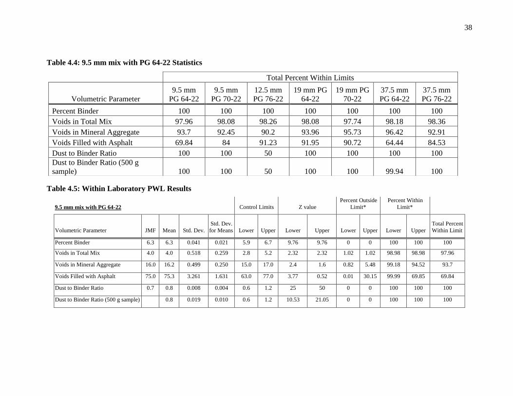
38

Table 4.4: 9.5 mm mix with PG 64-22 Statistics

Table 4.5: Within Laboratory PWL Results

9.5 mm mix with PG 64-22 Control Limits Z value

Percent Outside

Limit*

Percent Within

Limit*

Volumetric Parameter JMF Mean Std. Dev.

Std. Dev.

for Means Lower Upper Lower Upper Lower Upper Lower Upper

Total Percent

Within Limit

Percent Binder 6.3 6.3 0.041 0.021 5.9 6.7 9.76 9.76 0 0 100 100 100

Voids in Total Mix 4.0 4.0 0.518 0.259 2.8 5.2 2.32 2.32 1.02 1.02 98.98 98.98 97.96

Voids in Mineral Aggregate 16.0 16.2 0.499 0.250 15.0 17.0 2.4 1.6 0.82 5.48 99.18 94.52 93.7

Voids Filled with Asphalt 75.0 75.3 3.261 1.631 63.0 77.0 3.77 0.52 0.01 30.15 99.99 69.85 69.84

Dust to Binder Ratio 0.7 0.8 0.008 0.004 0.6 1.2 25 50 0 0 100 100 100

Dust to Binder Ratio (500 g sample) 0.8 0.019 0.010 0.6 1.2 10.53 21.05 0 0 100 100 100

Total Percent Within Limits

Volumetric Parameter

9.5 mm

PG 64-22

9.5 mm

PG 70-22

12.5 mm

PG 76-22

19 mm PG

64-22

19 mm PG

70-22

37.5 mm

PG 64-22

37.5 mm

PG 76-22

Percent Binder 100 100 100 100 100 100 100

Voids in Total Mix 97.96 98.08 98.26 98.08 97.74 98.18 98.36

Voids in Mineral Aggregate 93.7 92.45 90.2 93.96 95.73 96.42 92.91

Voids Filled with Asphalt 69.84 84 91.23 91.95 90.72 64.44 84.53

Dust to Binder Ratio 100 100 50 100 100 100 100

Dust to Binder Ratio (500 g

sample) 100 100 50 100 100 99.94 100

39

Table 4.5 show that percent binder, voids in the total mix, voids in the mineral aggregate,

and dust to binder ratio are not likely to fall outside the acceptable range set by the

WVDOH due to variations associated with the test method. Both Pb, VMA, and D/B

have a very high percent falling within the limits. The only exception is for the dust to

binder criteria for the 12.5 mm mix. The results show that the property only passes 50

percent of the time. This is due to the mix design showing the limits as 0.8 to 1.6, and the

mean being at 0.78. There is potentially a mistake in the mix design documents. In some

cases, the D/B criteria have a range of 0.6 to 1.2. If this is the case, the percent within

limits is 100%.

The questionable criteria limits occur for voids filled with asphalt. The range of

acceptable limits is 65 to 92 for VFA. These percent within limits are quite variable and

indicate that, in some cases, the variability due to the testing methods would cause

rejection of an acceptable material. These results support the decision by the WVDOH to

remove VFA from the quality control requirements (Epperly, 2003).

4.3.2 Effect of Varying Asphalt Content

The results of the simulations for varying the percent binder in a mix are

presented in Figure 4.1. In general, VMA is not affected enough by changes in Pb to

cause any chance of rejection based on the variation in the test methods alone. The D/B

is not dramatically affected in 5 of the 7 mix designs when the Pb is varied within

tolerance limits. However, it is clear that percent binder has a large impact on the VFA

results. VTM is also affected, but not as significantly as the VFA parameter.

The D/B results for the 37.5 mm with PG 64-22 binder in Figure 4.1(f) shows that

after an increase in Pb of more than one-tenth percent, there is not enough dust in the mix

to keep the dust to binder ratio above the lower limit. The other D/B exception is the

12.5-mm mix with PG 76-22 binder, Figure 4.1(c). As discussed above, the reason for

this high percent outside of the limits is likely due to an error in the mix design report.

The changing Pb does not show a change in acceptance of the D/B criteria, but instead the

results were only within limits fifty percent of the time.

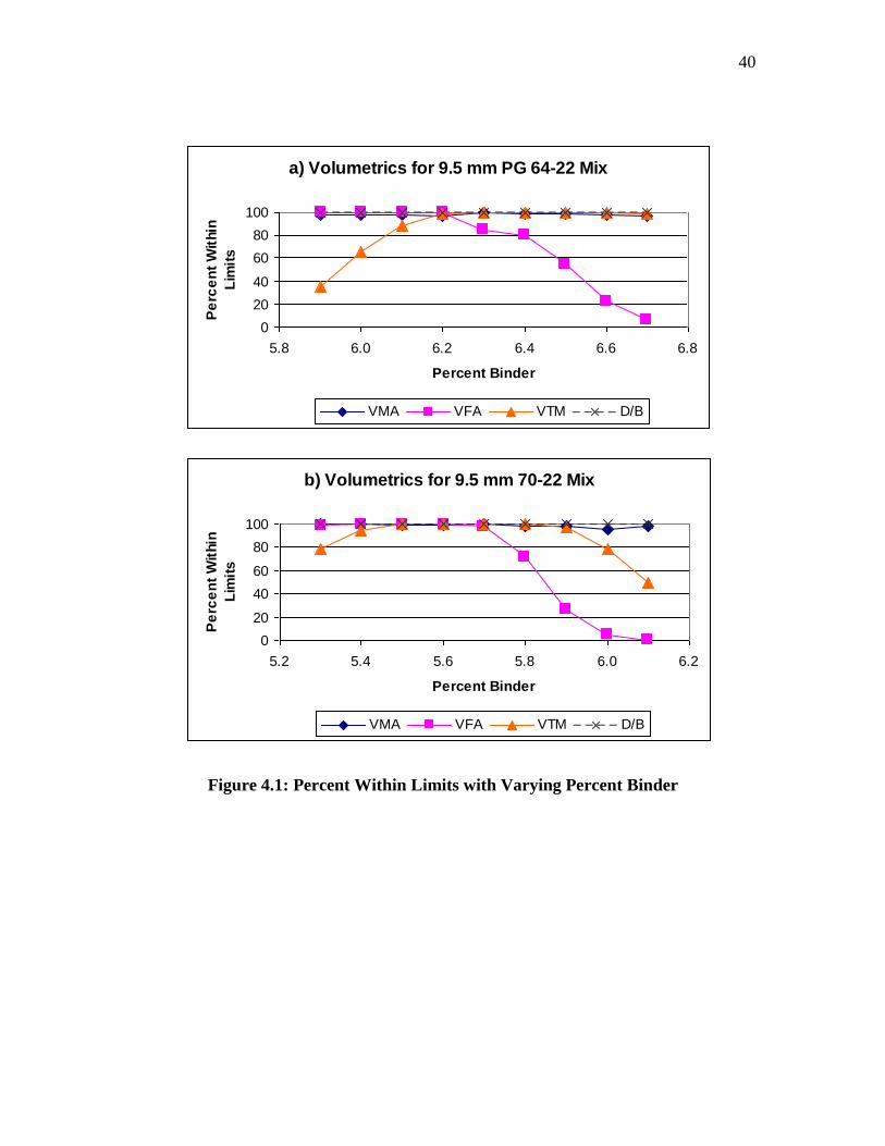
40

a) Volumetrics for 9.5 mm PG 64-22 Mix

0

20

40

60

80

100

5.8 6.0 6.2 6.4 6.6 6.8

Percent Binder

Pe

rce

nt

Wit

hin

Lim

its

VMA VFA VTM D/B

b) Volumetrics for 9.5 mm 70-22 Mix

0

20

40

60

80

100

5.2 5.4 5.6 5.8 6.0 6.2

Percent Binder

Pe

rce

nt

Wit

hin

Lim

its

VMA VFA VTM D/B

Figure 4.1: Percent Within Limits with Varying Percent Binder

41

c) Volumetrics for 12.5 mm 76-22 Mix

0

20

40

60

80

100

4.6 4.8 5.0 5.2 5.4 5.6

Percent Binder

Pe

rce

nt

Wit

hin

Lim

its

VMA VFA VTM D/B

d) Volumetrics for 19 mm 64-22 Mix

0

20

40

60

80

100

4.4 4.6 4.8 5.0 5.2 5.4

Percent Binder

Pe

rce

nt

Wit

hin

Lim

its

VMA VFA VTM D/B

e) Volumetrics for 19 mm 70-22 Mix

0

20

40

60

80

100

4.2 4.4 4.6 4.8 5.0 5.2 5.4

Percent Binder

Pe

rce

nt W

ithin

Lim

its

VMA VFA VTM D/B

Figure 4.1: Continued

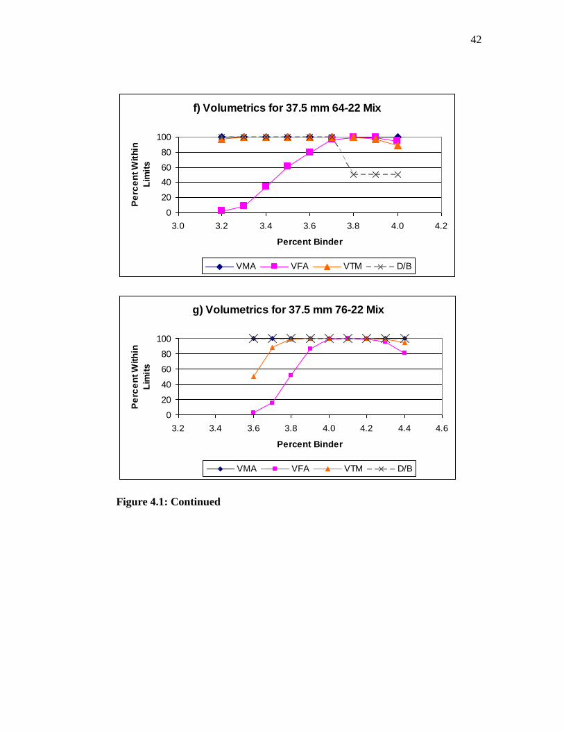
42

f) Volumetrics for 37.5 mm 64-22 Mix

0

20

40

60

80

100

3.0 3.2 3.4 3.6 3.8 4.0 4.2

Percent Binder

Pe

rce

nt W

ithin

Lim

its

VMA VFA VTM D/B

g) Volumetrics for 37.5 mm 76-22 Mix

0

20

40

60

80

100

3.2 3.4 3.6 3.8 4.0 4.2 4.4 4.6

Percent Binder

Pe

rce

nt W

ith

in

Lim

its

VMA VFA VTM D/B

Figure 4.1: Continued

43

The VFA showed the most variability in being accepted or rejected based on the

change in Pb. In most of the mixes, the VFA results would be likely to be rejected, as the

percent binder was varied from the accepted target value from the JMF. The figures also

show that the percent VFA within limits is sometimes higher for asphalt contents other

than the approved JMF value. In some cases, increasing or decreasing the percent binder

by one-tenth percent will increase the probability that tests will indicate the mix is within

the VFA specification limits. It appears that the percent within limits decreases as the

asphalt content is increased above the JMF value for the 9.5 mm mixes. The percent

within limits for VFA decreases with either an increase or decrease in asphalt content for

the 19 mm mixes. For the 37.5 mm mixes, the percent VFA within limits decreases for

asphalt contents less than the JMF target.

The results for VTM verses percent binder show somewhat of an umbrella-shape

effect. The acceptance of VTM remains high for the mixes as long as the Pb stays within

about two-tenths of the target Pb. However, if the change Pb exceeds two-tenths, then the

percent within limits of the VTM results decreases rapidly.

4.3.3 Quality Assurance Analysis

The results of the quality assurance analysis are presented in Table 4.6. The

statistics used for the development of the quality assurance analysis were based on a 1 in

20 chance that a test result would fail the criteria due to variability associated with

sampling and testing. The percent binder results in Table 4.6 demonstrate that, for this

parameter, the failure rate is reasonable if there are 10 quality control tests. If there are

fewer tests, the percent of tests that fall outside the acceptable range is reduced. This is

associated with the increase in the multiplier for the range used in Equation 2.1. For

fewer tests, the allowable range is increased. For the other quality control parameters, the

rate of rejection is much higher than expected. In general, when there are 10 quality

control tests the rate of rejection is as high as 20 percent or four times greater than

expected. It may be noted that the percent binder is determined directly from the ignition

oven test, so the development of criteria for the limits is fairly straightforward. The other

parameters, which show a higher rejection rates, are the result of multiple tests and,

therefore, the development of criteria is much more difficult. Table 4.6 also shows a

considerable difference in the rate of rejection for the D/B criteria based on the sample

44

size used to determine the gradation and, hence, the percent of aggregate passing the

0.075 mm sieve. The rejection rate of D/B is much greater when the P0.075 is determined

based on a 500 g sample.

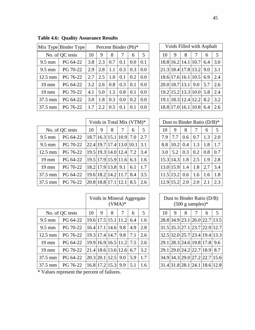
45

Table 4.6: Quality Assurance Results

Mix Type Binder Type Percent Binder (Pb)* Voids Filled with Asphalt

(VFA)* No. of QC tests 10 9 8 7 6 5 10 9 8 7 6 5

9.5 mm PG 64-22 3.8 2.3 0.7 0.1 0.0 0.1 18.8 16.2 14.1 10.7 6.4 3.0

9.5 mm PG 70-22 2.9 2.8 1.1 0.3 0.3 0.0 21.3 18.4 17.8 13.2 9.0 3.1

12.5 mm PG 76-22 2.7 2.5 1.0 0.1 0.2 0.0 18.6 17.6 16.1 10.5 6.9 2.4

19 mm PG 64-22 3.2 2.6 0.8 0.3 0.1 0.0 20.0 18.7 13.1 9.0 5.7 2.6

19 mm PG 70-22 4.1 5.0 1.5 0.8 0.1 0.0 19.2 15.2 13.3 10.0 5.8 2.4

37.5 mm PG 64-22 3.0 1.8 0.3 0.0 0.2 0.0 19.1 18.3 12.4 12.2 8.2 3.2

37.5 mm PG 76-22 1.7 2.2 0.5 0.1 0.1 0.0 18.8 17.0 16.1 10.8 6.4 2.6

Voids in Total Mix (VTM)* Dust to Binder Ratio (D/B)*

No. of QC tests 10 9 8 7 6 5 10 9 8 7 6 5

9.5 mm PG 64-22 18.7 16.3 15.1 10.9 7.0 2.7 7.9 7.7 0.6 0.7 1.3 2.0

9.5 mm PG 70-22 22.4 19.7 17.4 13.0 10.1 3.1 8.8 10.2 0.4 1.3 1.8 1.7

12.5 mm PG 76-22 19.5 19.3 14.0 12.4 7.2 3.4 3.0 5.2 0.3 0.2 0.8 0.7

19 mm PG 64-22 19.5 17.9 15.9 11.6 6.3 1.6 15.3 14.3 1.8 2.5 1.9 2.8

19 mm PG 70-22 18.2 17.9 13.8 9.1 6.1 1.7 13.0 15.9 1.4 1.8 2.7 3.4

37.5 mm PG 64-22 19.6 18.2 14.2 11.7 8.4 3.5 11.5 13.2 0.6 1.6 1.6 1.8

37.5 mm PG 76-22 20.8 18.8 17.1 12.1 8.5 2.6 12.9 15.2 2.0 2.0 2.1 2.3

Voids in Mineral Aggregate

(VMA)*

Dust to Binder Ratio (D/B)

(500 g samples)*

No. of QC tests 10 9 8 7 6 5 10 9 8 7 6 5

9.5 mm PG 64-22 19.6 17.5 15.1 11.2 6.4 1.6 28.8 34.9 23.1 26.0 22.7 13.5

9.5 mm PG 70-22 16.4 17.1 14.6 9.8 4.9 2.8 31.5 35.3 27.1 23.7 22.9 12.7

12.5 mm PG 76-22 19.3 17.4 14.7 9.8 7.1 2.6 32.5 32.0 25.7 23.4 19.4 13.3

19 mm PG 64-22 19.9 16.9 16.5 11.2 7.5 2.6 29.1 28.3 24.6 19.8 17.8 9.6

19 mm PG 70-22 21.4 18.6 13.6 12.6 6.7 3.2 29.1 29.0 24.2 22.7 18.9 8.7

37.5 mm PG 64-22 20.3 20.1 12.5 9.0 5.9 1.7 34.9 34.3 29.0 27.2 22.7 15.6

37.5 mm PG 76-22 16.8 17.2 15.3 9.9 5.1 1.6 31.4 31.8 28.1 24.1 18.6 12.8

* Values represent the percent of failures.

46

CHAPTER 5 CONCLUSIONS AND RECOMMENDATIONS

5.1 SUMMARY

Current practice of quality control for Superpave hot mix asphalt by WVDOH has

caused concern over the fairness of the specifications. The current specifications focus

on volumetric parameters as a means to evaluate the quality of hot mix asphalt concrete.

The research presented herein uses Monte Carlo simulation to determine the

probability that a quality control result will fall outside the acceptance limits based due to

the variability of the test methods. The quality control parameters used by the WVDOH

for Superpave mixes are the percent binder, voids in total mix, voids in mineral aggregate

and dust to binder ratio. When Superpave was introduced, voids filled with asphalt was

also a quality control parameter, so it was included in the research even though the

WVDOH has removed this requirement. Other states may still be using this parameter

and may benefit from the results produced during this analysis. The percent binder is the

only quality control parameter that is directly measured by testing. All of the other

parameters require multiple tests to determine their values. This complicates the

determination of the probability distribution function for the QC parameter in a

deterministic manner. Hence, the need to use a simulation tool was necessary. Monte

Carlo simulation has been used for evaluating the mix design process, but no citations

were found in the literature on using this tool to evaluate the QC/QA process.

MCS requires quantification of the probability distribution function for each of

the parameters included in the simulated result. AASHTO and ASTM test methods

include precision statements, which essentially define the standard deviation of the test

method. This implies that the test results are normally distributed. Assuming this is the

case, the probability distribution function for each test is defined by a mean and a

standard deviation. For this research, mean values for the tests were determined as the

target values for the parameter based on WVDOH approved mix designs. The precision

statement for each test method was used as the estimate of the standard deviation for a

test result. For the quality control parameters, which required multiple test procedures,

standard volumetric formulas were used to compute the resultant quality control

47

parameter. These functions were programmed into an Excel worksheet for performing

the Monte Carlo simulation. For the analysis of the quality control procedures, the

@Risk add-in program for Excel was used to simplify the development of the Monte

Carlo simulation. However, for the analysis of the quality assurance procedure it was

more expedient to develop a small Visual Basic for Applications program to perform the

Monte Carlo simulation.

Using the MCS, the quality control parameters were evaluated for seven different

combinations of mix types and binder grades. Each mix was evaluated separately for the

five quality control parameters.

5.2 CONCLUSIONS

The MCS of the quality control procedure demonstrated that variability in the test

methods and subsequent calculation of the quality control parameters does not overly

influence the determination of whether or not a mix has acceptable properties. If hot mix

asphalt is being produced with an asphalt content near the target value from the mix

design, there is less than a two percent chance that the test results will be outside of the

specification limits due to the variability in the testing methods. The voids filled with

asphalt parameter is an exception to this statement. In one case, there was a 35 percent

chance that a mix would fail the VFA criteria due to test method variability. However, if

there is a "drift" in the asphalt content by more than two-tenths percent, the potential for

rejecting the mix due to voids in the total mix being outside the specification limits

increases.

The MCS of the quality assurance process demonstrated it is not as robust as the

quality control process. The QC parameters, other than percent binder, can have a 20

percent or greater probability of rejection due to the variability in the test method,

especially if the QA result is tested against a range established from 10 QC tests. When a

QA test falls outside of the acceptable range, the WVDOH procedure is to investigate the

testing to determine if there was a flaw in either the QC or QA test methods or analysis.

This is a rather benign consequence and, hence, a high rejection rate may be acceptable.

In fact a periodic review of testing equipment, techniques and procedures is probably

beneficial to the overall quality control and assurance program.

48

The MCS of the quality control program indicates that the variability associated

with the Superpave quality control program is not causing undue errors of either

accepting bad mixes nor rejecting acceptable mixes. However, the quality assurance

process may be resulting in more reviews of the testing process than was intended when

the procedures were developed.

5.3 RECOMMENDATIONS

Based on the results of the Monte Carlo simulation of the WVDOH Monte Carlo

simulation it is recommended that the division continue with current quality control and

quality assurance practices. The quality control practices should not produce

unacceptable risk for accepting bad products or rejecting good products. The quality

assurance method can trigger an investigation into the quality control testing with a

greater frequency than would be reasonable for a quality control procedure. However,

since the consequence of finding differences between the contractors' quality control

results and the divisions quality assurance results is only to trigger a review of the test

methods, it is not unreasonable to use a "tight" criteria for this decision.

The WVDOH specifications allow a variation of 0.4% in the asphalt content

during construction. However, if the contractor allows the variance in asphalt content to

exceed 0.2% there is a risk that other volumetric parameters will trigger rejection of the

material due to the variability in the test methods.

This research did not examine the mix design process. Research by Hand and

Epps (2000) indicates there is an unacceptable variation in the design binder content

determined with the Superpave method due to the variability in the test methods. This

problem should be further investigated.

49

REFERENCES

1. ASTM Annual Book of ASTM Standards. Volume 4.02. West Conshohocken,

PA. (2000)

2. AASHTO Standard Specifications for Transportation Materials and Methods of

Sampling and Testing. Part I and Part II. Washington, D.C. (2000)

3. Cominsky, R.J. B.M. Killingsworth, R.M. Anderson, and D.A. Anderson,

"Quality Control and Acceptance of Superpave-Designed Hot Mix Asphalt",

Report 409, National Cooperative Highway Research Program, Washington D.C.

1998

4. Darlington, R. and Carlson, P., Behavior Statistics, The Free Press, 1975.

5. Decker, D.S. “How is Superpave Impacting the Contractor?” 2nd Eurasphalt &

Eurobitume Congress Barcelona 2000. Book I, 172-178.

http://www.eecongress.org/2000/pdfbook3/session1/proc0286uk.pdf (11/10/03)

6. Epperly, R., Letter to the West Virginia Contractors, July 23, 2003

7. Hand, A. and Epps, A. “Effects of Test Variability on Mixture Volumetrics and

Mix Design Verification”, Journal of the Association of Asphalt Paving

Technologists,Proceedings, Vol. 69, 2000, pp. 635-674, Washington, USA

8. Hutchinson, S. and Bandalos, D. A Guide to Monte Carlo Simulation Research

for Applied Researchers. Journal of Vocational Education Research, 22, 233-245.

(1997).

9. Newcomb, D.E., and Epps, J.A., January/February. “Statistical Specifications for

Hot Mix Asphalt: What Do We Need to Know” Hot Mix Asphalt Technology, 54-

59. (2001a)

10. Newcomb, D.E., and Epps, J.A., March/April. “Statistical Specifications for Hot

Mix Asphalt: What Do We Need to Know” Hot Mix Asphalt Technology, 37-40.

(2001b)

11. Palisade Corporation. @RISK Manual. (1997). Newfield, NY:

12. Peterson, J., Probability Analysis of Slope Stability, Master Thesis, West Virginia

University, Morgantown, WV 1999

13. Riegle, J., Development of an Integrated Project Level Pavement Management

Model Using Risk Analysis, Ph.D. Dissertation, West Virginia University,

Morgantown, WV, 2000

14. Roberts, F., Kandhal, P., Brown, E., Lee, D., and Kennedy, T. Hot Mix Asphalt

Materials, Mixture Design, and Construction. Second Edition, NAPA Research

and Education Foundation, 1996.

15. USDOE, “Introduction to Monte Carlo Methods”. U.S. Department of Energy.

Computational Science Education Project. http://csep1.phy.ornl.gov/mc/mc.html

(10/25/03)

50

16.

TEST METHODS AND MATERIAL PROCEDURES

AASHTO Test Methods

AASHTO PP-28

AASHTO R 9-97: Acceptance Sampling Plans for Highway Construction

AASHTO T 11-91: Materials Finer Than No. 200 Sieve in Mineral

Aggregates by Washing

AASHTO T 19/T 19M-00: Bulk Density and Voids in Aggregate

AASHTO T 27-99: Sieve Analysis of Fine and Coarse Aggregates

AASHTO T 30-98: Mechanical Analysis of Extracted Aggregate

AASHTO T 84-00: Specific Gravity and Absorption of Fine Aggregate

AASHTO T 85-96: Specific Gravity and Absorption of Coarse Aggregate

AASHTO T 164-97: Quantitative Extraction of Bituminous Paving Mixtures

AASHTO T 166-00: Bulk Specific Gravity of Compacted Asphalt Mixtures

Using Saturated Surface-Dry Specimens

AASHTO T 195: Determining Degree of Particle Coating of Bituminous-

Aggregate Mixtures

AASHTO T 209-99: Theoretical Maximum Specific Gravity and Density of

Bituminous Paving Mixtures

AASHTO T 240-97: Effect of Heat and Air on a Moving Film of Asphalt

(Rolling Thin Film Oven)

AASHTO T 269-97: Percent Air Voids in Compacted Dense and Open

Bituminous Paving Mixtures

AASHTO T304-00: Uncompacted Void Content of Fine Aggregate

AASHTO T308-99 (METHOD A): Determining the Asphalt Binder Content

of Hot-Mix Asphalt by Ignition Method

51

AASHTO T312: Preparing and Determining the Density of Hot-Mix Asphalt

Specimens by Means of the Superpave Gyratory Compactor

ASTM Test Methods

ASTM C 670-96: Preparing Precision and Bias Statements for Test Methods

for Construction Materials

ASTM D5821-95: Determining the Percentage of Fractured Faces in Coarse

Aggregate

ASTM D70-90: Specific Gravity and Density of Semi-Solid Bituminous

Materials

WVDOH Material Procedures

Material Procedures. West Virginia Division of Transportation.

http://www.wvdot.com/10_contractors/10f7_procedures.htm (10/20/03)

401.02.29: Guideline for Quality Control and Acceptance Requirements

for Superpave Hot-Mix Asphalt

401.03.50: Guide for Contractor's Quality Control of Bituminous Concrete

700.00.54: Procedure for Evaluating Quality Control Sample Test Results

with Verification Sample Test Results

52

APPENDIX 1 MONTE CARLO SIMULATION RESULTS

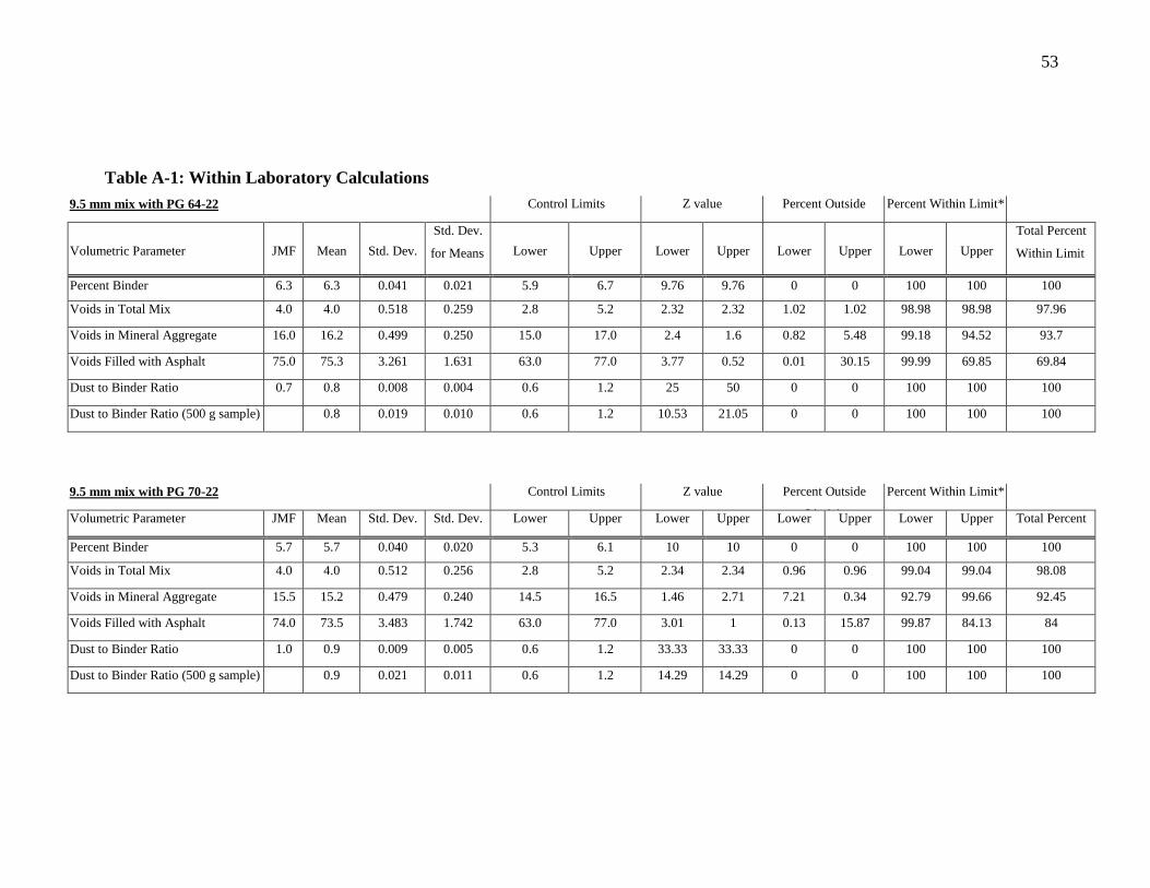
53

Table A-1: Within Laboratory Calculations

9.5 mm mix with PG 64-22 Control Limits Z value Percent Outside

Limit*

Percent Within Limit*

Volumetric Parameter JMF Mean Std. Dev.

Std. Dev.

for Means Lower Upper Lower Upper Lower Upper Lower Upper

Total Percent

Within Limit

Percent Binder 6.3 6.3 0.041 0.021 5.9 6.7 9.76 9.76 0 0 100 100 100

Voids in Total Mix 4.0 4.0 0.518 0.259 2.8 5.2 2.32 2.32 1.02 1.02 98.98 98.98 97.96

Voids in Mineral Aggregate 16.0 16.2 0.499 0.250 15.0 17.0 2.4 1.6 0.82 5.48 99.18 94.52 93.7

Voids Filled with Asphalt 75.0 75.3 3.261 1.631 63.0 77.0 3.77 0.52 0.01 30.15 99.99 69.85 69.84

Dust to Binder Ratio 0.7 0.8 0.008 0.004 0.6 1.2 25 50 0 0 100 100 100

Dust to Binder Ratio (500 g sample) 0.8 0.019 0.010 0.6 1.2 10.53 21.05 0 0 100 100 100

9.5 mm mix with PG 70-22 Control Limits Z value Percent Outside

Limit*

Percent Within Limit*

Volumetric Parameter JMF Mean Std. Dev. Std. Dev.

for Means

Lower Upper Lower Upper Lower Upper Lower Upper Total Percent

Within Limit Percent Binder 5.7 5.7 0.040 0.020 5.3 6.1 10 10 0 0 100 100 100

Voids in Total Mix 4.0 4.0 0.512 0.256 2.8 5.2 2.34 2.34 0.96 0.96 99.04 99.04 98.08

Voids in Mineral Aggregate 15.5 15.2 0.479 0.240 14.5 16.5 1.46 2.71 7.21 0.34 92.79 99.66 92.45

Voids Filled with Asphalt 74.0 73.5 3.483 1.742 63.0 77.0 3.01 1 0.13 15.87 99.87 84.13 84

Dust to Binder Ratio 1.0 0.9 0.009 0.005 0.6 1.2 33.33 33.33 0 0 100 100 100

Dust to Binder Ratio (500 g sample) 0.9 0.021 0.011 0.6 1.2 14.29 14.29 0 0 100 100 100

54

12.5 mm mix with PG 76-22 Control Limits Z value Percent Outside

Limit*

Percent Within Limit*

Volumetric Parameter JMF Mean Std. Dev. Std. Dev.

for Means

Lower Upper Lower Upper Lower Upper Lower Upper Total Percent

Within Limit Percent Binder 5.1 5.1 0.040 0.020 4.7 5.5 10 10 0 0 100 100 100

Voids in Total Mix 4.0 4.0 0.504 0.252 2.8 5.2 2.38 2.38 0.87 0.87 99.13 99.13 98.26

Voids in Mineral Aggregate 14.5 14.1 0.462 0.231 13.5 15.5 1.3 3.03 9.68 0.12 90.32 99.88 90.2

Voids Filled with Asphalt 70.0 71.8 3.688 1.844 63.0 77.0 2.39 1.41 0.84 7.93 99.16 92.07 91.23

Dust to Binder Ratio 1.0 0.8 0.010 0.005 0.8 1.6 0 80 50 0 50 100 50

Dust to Binder Ratio (500 g sample) 0.8 0.023 0.012 0.8 1.6 0 34.78 50 0 50 100 50

19 mm mix with PG 64-22 Control Limits Z value Percent Outside

Limit*

Percent Within Limit*

Volumetric Parameter JMF Mean Std. Dev. Std. Dev.

for Means

Lower Upper Lower Upper Lower Upper Lower Upper Total Percent

Within Limit Percent Binder 4.9 4.9 0.040 0.020 4.5 5.3 10 10 0 0 100 100 100

Voids in Total Mix 4.0 4.0 0.513 0.257 2.8 5.2 2.34 2.34 0.96 0.96 99.04 99.04 98.08

Voids in Mineral Aggregate 13.7 13.5 0.495 0.248 12.7 14.7 1.62 2.42 5.26 0.78 94.74 99.22 93.96

Voids Filled with Asphalt 71.0 70.2 3.992 1.996 63.0 77.0 1.8 1.7 3.59 4.46 96.41 95.54 91.95

Dust to Binder Ratio 1.3 1.1 0.009 0.005 0.6 1.2 55.56 11.11 0 0 100 100 100

Dust to Binder Ratio (500 g sample) 1.1 0.025 0.013 0.6 1.2 20 4 0 0 100 100 100

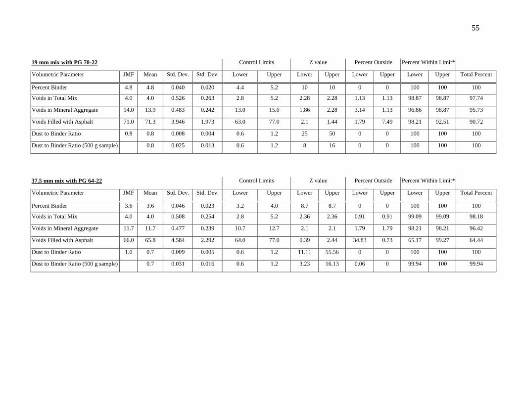
55

19 mm mix with PG 70-22 Control Limits Z value Percent Outside

Limit*

Percent Within Limit*

Volumetric Parameter JMF Mean Std. Dev. Std. Dev.

for Means

Lower Upper Lower Upper Lower Upper Lower Upper Total Percent

Within Limit Percent Binder 4.8 4.8 0.040 0.020 4.4 5.2 10 10 0 0 100 100 100

Voids in Total Mix 4.0 4.0 0.526 0.263 2.8 5.2 2.28 2.28 1.13 1.13 98.87 98.87 97.74

Voids in Mineral Aggregate 14.0 13.9 0.483 0.242 13.0 15.0 1.86 2.28 3.14 1.13 96.86 98.87 95.73

Voids Filled with Asphalt 71.0 71.3 3.946 1.973 63.0 77.0 2.1 1.44 1.79 7.49 98.21 92.51 90.72

Dust to Binder Ratio 0.8 0.8 0.008 0.004 0.6 1.2 25 50 0 0 100 100 100

Dust to Binder Ratio (500 g sample) 0.8 0.025 0.013 0.6 1.2 8 16 0 0 100 100 100

37.5 mm mix with PG 64-22 Control Limits Z value Percent Outside

Limit*

Percent Within Limit*

Volumetric Parameter JMF Mean Std. Dev. Std. Dev.

for Means

Lower Upper Lower Upper Lower Upper Lower Upper Total Percent

Within Limit Percent Binder 3.6 3.6 0.046 0.023 3.2 4.0 8.7 8.7 0 0 100 100 100

Voids in Total Mix 4.0 4.0 0.508 0.254 2.8 5.2 2.36 2.36 0.91 0.91 99.09 99.09 98.18

Voids in Mineral Aggregate 11.7 11.7 0.477 0.239 10.7 12.7 2.1 2.1 1.79 1.79 98.21 98.21 96.42

Voids Filled with Asphalt 66.0 65.8 4.584 2.292 64.0 77.0 0.39 2.44 34.83 0.73 65.17 99.27 64.44

Dust to Binder Ratio 1.0 0.7 0.009 0.005 0.6 1.2 11.11 55.56 0 0 100 100 100

Dust to Binder Ratio (500 g sample) 0.7 0.031 0.016 0.6 1.2 3.23 16.13 0.06 0 99.94 100 99.94

56

37.5 mm mix with PG 76-22 Control Limits Z value Percent Outside

Limit*

Percent Within Limit*

Volumetric Parameter JMF Mean Std. Dev. Std. Dev.

for Means

Lower Upper Lower Upper Lower Upper Lower Upper Total Percent

Within Limit Percent Binder 4.0 4.0 0.041 0.021 3.6 4.4 9.76 9.76 0 0 100 100 100

Voids in Total Mix 4.0 4.0 0.500 0.250 2.8 5.2 2.4 2.4 0.82 0.82 99.18 99.18 98.36

Voids in Mineral Aggregate 13.0 12.7 0.470 0.235 12.0 14.0 1.49 2.77 6.81 0.28 93.19 99.72 92.91

Voids Filled with Asphalt 68.0 68.6 4.144 2.072 64.0 77.0 1.11 2.03 13.35 2.12 86.65 97.88 84.53

Dust to Binder Ratio 1.0 1.0 0.010 0.005 0.8 1.6 20 60 0 0 100 100 100

Dust to Binder Ratio (500 g sample) 1.0 0.030 0.015 0.8 1.6 6.67 20 0 0 100 100 100

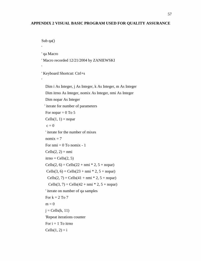
57

APPENDIX 2 VISUAL BASIC PROGRAM USED FOR QUALITY ASSURANCE

Sub qa()

'

' qa Macro

' Macro recorded 12/21/2004 by ZANIEWSKI

'

' Keyboard Shortcut: Ctrl+s

'

Dim i As Integer, j As Integer, k As Integer, m As Integer

Dim itrno As Integer, nomix As Integer, nmi As Integer

Dim nopar As Integer

' iterate for number of parameters

For nopar = 0 To 5

Cells(1, 1) = nopar

c = 0

' iterate for the number of mixes

nomix = 7

For nmi = 0 To nomix - 1

Cells(2, 2) = nmi

itrno = Cells(2, 5)

Cells(2, 6) = Cells(22 + nmi * 2, 5 + nopar)

Cells(3, 6) = Cells(23 + nmi * 2, 5 + nopar)

Cells(2, 7) = Cells(41 + nmi * 2, 5 + nopar)

Cells(3, 7) = Cells(42 + nmi * 2, 5 + nopar)

' iterate on number of qa samples

For k = 2 To 7

m = 0

j = Cells(k, 11)

'Repeat iterations counter

For i = 1 To itrno

Cells(1, 2) = i

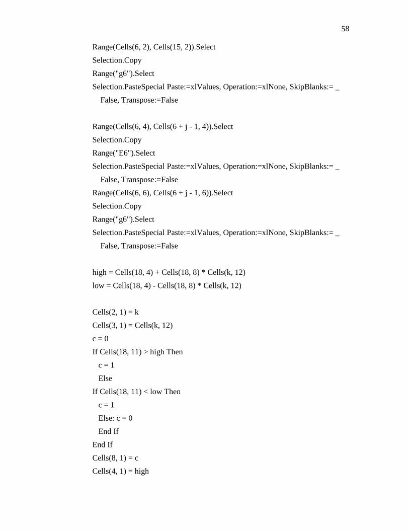
58

Range(Cells(6, 2), Cells(15, 2)).Select

Selection.Copy

Range("g6").Select

Selection.PasteSpecial Paste:=xlValues, Operation:=xlNone, SkipBlanks:= _

False, Transpose:=False

Range(Cells(6, 4), Cells(6 + j - 1, 4)).Select

Selection.Copy

Range("E6").Select

Selection.PasteSpecial Paste:=xlValues, Operation:=xlNone, SkipBlanks:= _

False, Transpose:=False

Range(Cells(6, 6), Cells(6 + j - 1, 6)).Select

Selection.Copy

Range("g6").Select

Selection.PasteSpecial Paste:=xlValues, Operation:=xlNone, SkipBlanks:= _

False, Transpose:=False

high = Cells(18, 4) + Cells(18, 8) * Cells(k, 12)

low = Cells(18, 4) - Cells(18, 8) * Cells(k, 12)

Cells(2, 1) = k

Cells(3, 1) = Cells(k, 12)

c = 0

If Cells(18, 11) > high Then

c = 1

Else

If Cells(18, 11) < low Then

c = 1

Else: c = 0

End If

End If

Cells(8, 1) = c

Cells(4, 1) = high

59

Cells(5, 1) = low

Cells(6, 1) = Cells(18, 11)

m = m + c

Cells(7, 1) = m

Next i

Cells(22 + nmi * 2, 13 + k - 2 + nopar * 6) = m

Cells(1, 13) = i - 1

Next k

Next nmi

Next nopar

End Sub