EVALUATION OF PARALLEL IMPLEMENTATION OF DENSE AND SPARSE

MATRIX FOR SCLATION LIBRARY

by

YUNG LONG LI

(Under the Direction of John A. Miller)

ABSTRACT

Many simulation and scientific programs frequently use basic linear algebra

operations, such as vector dot product and matrix multiplication. For instance, the Quasi

Newton method and Markov clustering algorithms make use of vector and matrices in

their code. Many of these problems require substantial amounts of processing time. One

possible way to save time is to execute the computations in parallel. In the early of 1970s,

MIMD multiprocessors (e.g., C.mmp) were introduced to speed up the execution of

programs, while later in that decade, cluster computing (e.g., ARCnet) also started to be

used to speed up the execution of programs. Today, mainstream parallel computing is

beginning to focus on utilizing multi-core processors. However, it is not easy for a

programmer to achieve acceptable performance both at the core level and at the cluster

level.

This report presents the design and implementation of two parallel structures,

MatrixD and SparseMatrixD, for the library of ScalaTion, which can be efficiently

executed in parallel at the core level. MatrixD and SparseMatrixD utilize Scala’s parallel

collection framework to achieve good performance at the core level. They can be used as

a regular matrix structure without any modification in the code and can result in

considerable speedup. An implementation that explores parallelism at the cluster level

utilizing the remote actor capabilities of Akka was shown to further improve performance.

The message passing model used by Akka provides programmers with an easy means to

implement parallelism in distributed systems. In this report, we study and implement a

Markov Clustering application. Testing the application on a large collaboration network

resulted in substantial speedup both at the core and cluster levels.

INDEX WORDS: Parallel Computing, Scala, Akka, ScalaTion, Matrix Multiplication,

Dense Matrix, Sparse Matrix, multiple cores, cluster.

EVALUATION OF PARALLEL IMPLEMENTATION OF DENSE AND SPARSE

MATRIX FOR SCLATION LIBRARY

by

YUNG LONG LI

MS, National Chung Hsing University, Taiwan, 2000

A Technical Report Submitted to the Computer Science for the Degree

MASTER OF SCIENCE

ATHENS, GEORGIA

2012

© 2012

YUNG LONG LI

All Rights Reserved

EVALUATION OF PARALLEL IMPLEMENTATION OF DENSE AND SPARSE

MATRIX FOR SCLATION LIBRARY

by

YUNG LONG LI

Major Professor: John A. Miller

Committee: Thiab Taha Krzysztof J. Kochut Electronic Version Approved: Maureen Grasso Dean of the Graduate School The University of Georgia "[May, August, or December]" "[Year of Graduation]"

iv

DEDICATION

To my family and friends.

v

ACKNOWLEDGEMENTS

I am greatly thankful to my major professor, Dr. Miller for his continuous support

and guidance during my study at UGA. He is a wonderful professor and always

encourages his students. I would also like to thank Dr. Thiab Taha and Dr. Kochut, for

their valuable suggestions and support. Finally, I would like to thank my colleagues and

friends who have helped me on this report.

vi

TABLE OF CONTENTS

Page

ACKNOWLEDGEMENTS .................................................................................................v

LIST OF TABLES ........................................................................................................... viii

LIST OF FIGURES ........................................................................................................... ix

CHAPTER

1 INTRODUCTION .............................................................................................1

2 OVERVIEW OF PARALLEL COMPUTING ..................................................5

2.1 BACKGROUND .....................................................................................5

2.2 PARALLEL COLLECTION IN SCALA .................................................7

2.3 AKKA TOOLKIT API FOR DISTRIBUTED SYSTEM .......................17

3 RELATED WORK ..........................................................................................21

3.1 GOOGLE MAPREDUCE ON MATRIX MULTIPLICATION .........21

3.2 PSBLAS ..............................................................................................22

4 EVALUATION IN PARALLEL COMPUTING ............................................23

4.1 ENVIRONMENT ................................................................................23

4-2 VECTOR DOT FOR PARALLEL ......................................................23

4-3 DENSE MATRIX OPERATION IN PARALLEL COMPUTING ....25

4-4 SPARSE MATRIX OPERATION IN PARALLEL COMPUTING ...32

4-5 DISTRIBUTED MATRIX MULTIPLICATION IN PARALLEL

COMPUTING ............................................................................................34

4.6 PERFORMANCE OF THE APPLICATIONS ....................................38

vii

5 CONCLUSIONS AND THE FUTURE WORK .............................................42

REFERENCES ..................................................................................................................44

APPENDIX ....................................................................................................................46

viii

LIST OF TABLES

Page

Table 1: overview of common data structure in sparse matrix ..........................................15

Table 2: test environment of every machine ......................................................................23

Table 3: dense matrix addition running time in different dimension and core number .....39

Table 4: dense matrix multiplication running time in different dimension and core

number .................................................................................................................39

Table 5: dense matrix inversion in different dimension and core number ........................39

Table 6: dense matrix LU decomposition in different dimension and core number .........40

Table 7: sparse matrix addition in different dimension and core number .........................40

Table 8: sparse matrix multiplication in different dimension and core number ................40

Table 9: dense matrix multiplication in different dimension in cluster .............................41

ix

LIST OF FIGURES

Page

Figure 1: exponential splitting process ................................................................................9

Figure 2: computation time of matrix multiplication with different dimension ................18

Figure 3: computation time of vector dot with different granularity .................................24

Figure 4: matrix parallel addition operation in different dimension ..................................26

Figure 5: matrix parallel multiplication in different dimension .........................................27

Figure 6: matrix parallel transpose & multiplication in different dimension ....................28

Figure 7: matrix parallel multiplication speedup in different dimension ..........................29

Figure 8: matrix parallel Strassen multiplication speedup in different dimension ............30

Figure 9: matrix parallel inversion in different dimension ................................................31

Figure 10: matrix parallel LU decomposition in different dimension ...............................32

Figure 11: sparse matrix parallel addition operation in different dimension .....................32

Figure 12: sparse matrix parallel multiplication in different dimension............................33

Figure 13: process of the data passing in cluster level .......................................................36

Figure 14: dense matrix parallel multiplication of cluster in different dimension ............37

Figure 15: sparse matrix parallel multiplication of cluster in different dimension............37

1

CHAPTER 1

INTRODUCTION

In computer science [01], serious interest of parallel computing started at the 1960.

Typically, the parallel machines of that era had multiple processors working on shared

memory. In the next years, there were some objections and cautionary statements which

slowed the progress in parallel computing. The most famous one is Amdahl’s law. It

states that a small fraction f of sequential computation was limited by the following rule.

Speed-up ≦ 1/[f + (1-f)/p]

Where, p is the number of processor and f is fraction of a program that cannot be

parallelized. It means that the speed-up will never exceed 1/f. Starting in the late 80’s,

cluster systems came to attract with more attention and were applied on many

applications. A cluster is a kind of parallel computer built with a numbers of computers

connected by a network. Today, cluster systems are popular in most scientific computing

area and are the dominant architecture in the data centers. Now, the trend starts to move

to multi-core processors. This is because increasing microprocessor will be more cost-

efficient than increasing clock frequencies. Today most desktop and laptop systems are

built with multi-core microprocessors. The manufacturers start to increase overall

performance by adding additional CPU cores. Therefore, parallel computing has to

consider utilizing the power of computing at the core level as well as at the cluster level.

These requirements make writing an efficient parallel program challenging for regular

programmer.

2

In order to overcome these challenging, many algorithm and techniques are

invented to ease the burden of a programmer. In sequential programming, there are many

collection frameworks have been implemented in order to provide optimal procedures for

sorting, filtering, and finding elements. In general, software is written for serial

computation, where only one instruction may execute at time. These frameworks usually

traverse the entire collection and process the elements sequentially using iterators. There

are many applications and data structure is used in the collection frameworks. The basic

structure linear algebra data structure, including vectors or matrice may use a collection

framework. Therefore, these linear algebra data structures can have a better performance

by using the parallel collection framework. Parallel computing techniques are designed

to utilize multiple compute resources to traverse different parts of data simultaneously,

resulting in a speed up. There are several reasons to use parallel computing such as

saving time and money, solving larger problems or using of the resources in a distributed

system. However, parallel programming is generally difficult and complicated. Therefore,

there is a need for a simple way to express the parallel computing problems that yields for

the non-expert scientist. The speed up is now becoming more and more important as the

larger data sets are used and stored in different sites. For example, BGI [02], which is the

world's largest genomics research laboratory, finds more that 2000 human genomes per

day. This data deluge is placing unprecedented demands on the data storage and data

processing infrastructures of bio-informatics research facilities around the world. To ease

the process of writing software that deals with big data, an efficient and simple way to

express parallel programming tasks is essential.

3

Recent research shows that faster networks, distributed systems and multi-

processor computer architectures are showing that wide use of parallelism is the possible

solution in the future of computing. There are several methods to implement parallel

computing. In this paper, we will focus on using a parallel collection framework and

distributed memory / message passing model approach where a set of tasks with their

own local memory are executed in parallel. Multiple tasks can reside on the same

physical machine and/or across an arbitrary number of machines. To alleviate the

programmer burden, an efficient parallel collection library could be used. The modern

programming language, Scala [03], contains a parallel collection framework that can

facilitate parallel computing without the need to manage the complexity of multiple

threads and the load balance problem. However, parallel computation may result in

unacceptable or incorrect outcome if these are used inappropriately. Most of time,

inappropriate use is because the programmers are continuing to think of the parallel

computing program as a sequential program. This can lead to inefficient performance,

and even an incorrect answer. In this paper, parallel frameworks will be implemented to

create in several different data structures, and explore an easy way to get optimal

performance. The vector and matrix structures are data structures which are often used in

other applications. If computation using these data structure can be executed in parallel,

then the process time can be saved. The basic linear algebra data structures, MatrixD and

SparseMatrixD, in the ScalaTion library, are implemented to use the parallel collection

framework to obtain improved performance. These two data structures take advantage of

the parallel collection framework so that the user can easily use them without the need of

writing extra code. Moreover, they can be used as the building block for other application

4

or software in a distributed system. In order to show the capability of these two data

structures, powerful toolkit, Akka [04], that is written in Scala and used for building

highly concurrent and distributed system without considering the low level task, such as

domain or specify the information in data structure, in message passing is an ideal

solution for building distributed systems. Scala is a cross-platform language; therefore,

Akka can be implemented in a networked cluster with different platforms. In this paper, a

networked cluster node system is implemented with Akka and the ScalaTion [05] library

to test dense matrix and sparse matrix multiplication speedup in cluster level.

The rest of the technical report is organized as follows. Chapter 2 gives an

overview of parallel computation and introduces the Scala language. Chapter 3 discusses

the related work. Chapter 4 compares the results of sequential and parallel computing in

dense matrices and sparse matrices and chapter 5 discusses relevant high level program

language features in Scala. Chapter 6 covers the conclusions and future work.

5

CHAPTER 2

OVERVIEW OF PARALLEL COMPUTING

2.1 BACKGROUND

For a long time, parallel programming was considered as a professional skill,

relevant only to high-performance applications. Now that big data and intensive

computation are more and more common in applications, parallel computation is

becoming a promising solution. In the future, future multi-core/many-core hardware will

not be slightly parallel, like today’s dual-core and quad-core processor architectures, but

will be massively parallel [06]. However, there are still many challenges in parallel

programming for a regular programmer who is only familiar with traditional sequential

programming.

It is not enough simply to permit parallelism in programs and expect a speedup to

be obtained. Programmers must think about parallelism as a fundamental part of their

program structure, just as they do with loops, conditionals in a sequential language. In the

report [06] which discusses about parallel computing issue, the key challenges or

problems include:

a. Decomposition and combination: the parallel tasks within the program must be

identified. If there is a return value, then a join operation is needed.

b. Race conditions: the order in which expressions are evaluated and/or the order of

communications may affect the outcome of the parallel program.

c. Locking: Shared memory locations must be locked to avoid conflicts that could

give inconsistent results; this locking is often expensive and very error-prone.

6

d. Granularity: Granularity is the extent to which a system is broken down into

small parts. It is necessary to achieve the correct level of granularity. Too fine-

grained or too coarse-grained system all lead to an inefficient performance.

Unfortunately, there is no general fixed choice to fit all situations.

e. Scalability: programs should scale to take advantage of increased numbers of

parallel processors.

f. Load balancing: work may be unevenly distributed among the available

processing resources, especially where tasks have irregular granularity. It may be

necessary to rebalance the work allocation.

All of these challenges need consideration when developing an efficient parallel

program. In [07], the advent of multi-core technology leads to a trend that indicates that

high-end parallel machine architectures which include a networked cluster of nodes, each

having a number of processor cores. It is known as distributed memory passing model.

In a distributed memory system, the above problems should be considered at two levels,

the core level and cluster level. At the core level, it is not necessary for the processes

distributed among the cores to consider the time of message passing, as this time is

usually very small. The most important challenge is to avoid conflicts which may lead to

an incorrect result. However, as the data size grows, this too large data problem is nearly

impossible to handle in a single machine. Parallel computing is necessary to solve this

problem in a distributed system. At the cluster level, the tasks are divided into many

small subtasks and each subtask is solved by a single machine. Today’s modern

programming languages have developed some useful frameworks to help programmers to

develop an efficient parallel application. In Brightwell and Heroux [6], they present

7

Parallel Phase Model(PPM), a unified high-level programming abstraction is presented,

and that facilitates the design and implementation of parallel algorithms to exploit both

parallelism of the many cores and the parallelism at the cluster level. In the past,

developing applications for these machines was more difficult than it is today, because

programmers needed to simultaneously exploit core-level parallelism (many cores and

shared memory) and cluster-level parallelism (distributed memory) to achieve good

application performance. However, even though program can be written to execute in

parallel and avoid conflicts in computation, they do not always to achieve an acceptable

performance, sometimes performing worse than their sequential implementation. This is

because inappropriate parallel implementation can cause problems in decomposition,

granularity and load balancing. Fortunately, today it is possible to utilize modern

programming languages and their parallel collections frameworks to solve such issues

more easily. In the next section, the modern programming language, Scala, and its

parallel collection feature, ParRange, are introduced, which can be used to make

efficient parallel implementations. The processes of how to develop efficient parallel

computation will be introduced and parallel design issue will be explored.

2.2 PARALLEL COLLECTION IN SCALA

In Prokopec report [08], it states “Scala is a modern general purpose statically typed

programming language which fuses object-oriented and functional programming”.

Operations are performed using the collection framework so dividing work can be done

by partitioning the collection into subsets. To perform parallel computing, it requires

dividing work to many small pieces and assigning subsets of elements to different

8

processors. However, creating and initializing a thread system is not free and it may

cause the extra cost by several orders of magnitude. Therefore, it is necessary to use pool

of worker threads in sleeping state to avoid creation each time as a parallel operation is

invoked. The parallel collection frameworks were introduced to ease the complication in

program. In Scala, it has implemented in ParRange. The most important algorithm

inside the ParRange is the Java Fork/Join Framework [9].

The general design in Fork/Join algorithm is a variant of the Work−Stealing [10]

algorithm. Fork/join algorithms are parallel versions of divide and conquer algorithms.

The Fork operation starts a new parallel subtask. The Join operation causes the current

task not to proceed until all its subtasks are completed. Like other divide-and-conquer

algorithms, it is recursive. It recursively divides the task until it is small enough to solve,

and then solve it sequentially. This framework manages a pool of worker threads, each

being assigned a queue of fork/join tasks. Normally, there are as many worker threads as

there are cores on a system [11]. Every subtask is executed by a thread in this pool. The

Work-Steal Algorithm plays an important role on Fork/Join Algorithm. Each worker

thread maintains runnable tasks in its own scheduling queue. When a worker thread has

no local tasks to run, it attempts to take ("steal") a task from another randomly chosen

worker, using a First In, First Out (oldest first) rule. The Work−Stealing algorithm helps

to deal with the load balance issue. In practice, fewer tasks usually lead to significant

performance improvement if subtask size is equal and every processor’s capabilities are

equal. However, if it is not, fewer tasks may lead to poorer load-balancing problem. In

[7], these issues are solved via exponential task splitting, inspired by [12]. The idea is the

following:

9

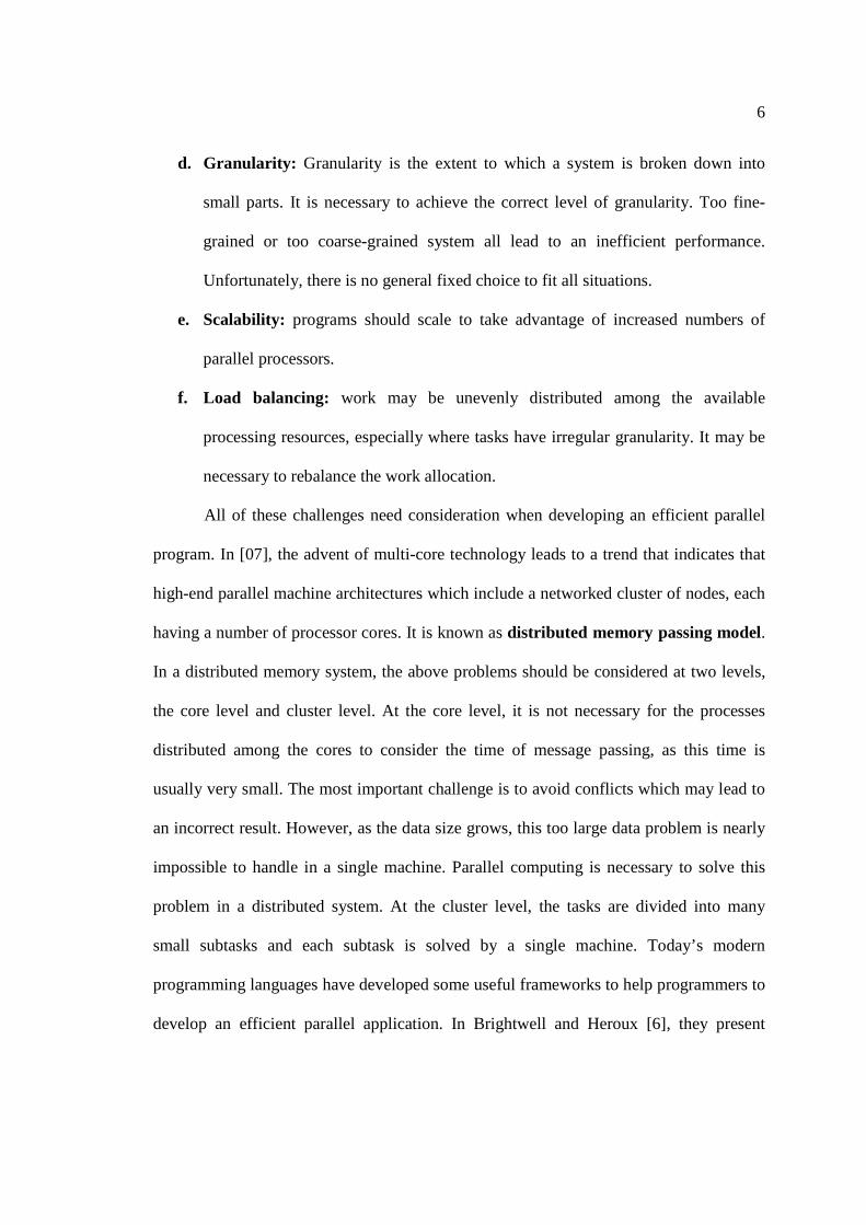
If a worker thread finished its work with more tasks in its queue, then it means that other

thread are busy with their own work, so the worker thread will do more tasks. The

heuristic is to double the amount of work. There are two advantages of this approach.

First, it allows only the oldest tasks on the queue to be stolen. Second, stealing tasks is

generally more expensive than just assigning them to the queue. The figure 1 shows the

exponential splitting process.

Figure 1 exponential task splitting process

The Scala parallel collections framework uses this process to efficiently schedule

tasks between cores/processors. ParRange, a parallel collection data structure in Scala,

is implemented by using Fork/Join framework of Java. ParRange is developed with

these algorithms and parallelizes well. The following code gives a simple example,

demonstrating how to use the ParRange.

3. Double size

Queue

1. Finish one task 2. Too many tasks remaining

10

for (i <- 0 until 100) process(i) -- regular range

for (i <- (0 until 100).par) process(i) -- parallel range

With ParRange, a programmer can easily implement a parallel process without

thinking about the low level tasks, such as creation of threads or the management of

threads. It can be an ideal solution for parallelization at the core level, because

programmers can be free from developing a complicated thread pool and handling the

load balancing issues.

Although Fork/Join can help us to deal with most of problems, we still need to

face some critical issues. An efficient and correct execution schedule may depend on

some factors which may include the number of processors, data size or processor

availability. In order to get a clear view on these problems, we use the vector dot product

operator as an example in order to demonstrate a parallel programming problem and how

to solve it.

The dot product is a binary operation that takes two equal-length sequences of

vectors and produces a single number by multiplying corresponding entries in each input

vector and summing those products. This function can be easily implemented by a for-

loop which adapts a normal for-loop. A naïve way to produce a parallel implementation

is to replace the normal Range by ParRange, see the following code.

11

def dot (b: VectorD): Double =

{

var s = 0.0

for (i <- (0 until dim).par) s += v(i) * b(i)

s // return

} // dot

After the execution of the dot method, in a 4-cores machine, the measurement of

parallel performance shows only 40 percent faster than previous measurement and it

generates an incorrect result. The example demonstrates how the parallel collect

framework can be misused. The incorrect response is due to shared memory not being

locked as every thread writes the value in variable “s” value. This case demonstrates a

critical issue about the kind of functional language used in parallel programming. In pure

functional programming languages, a programmer is prevented from using mutable

variable in their program. An important reason for using functional language is because

there are no side effects, so it is always safe to execute computations in parallel due to

this referential transparency. Without mutable variables, the program can be decomposed

and run in order safely. Scala encourages users not to use mutable variables and supports

many functional programming paradigms that can be used to avoid using mutable

variable. To solve this problem, we assign a simple array to make our parallel

“ParRange” to write the same value concurrently. The code is then modified as

following

12

def dot (b: VectorD): Double =

{

val arr = new Array[Double](dim)

for (i <- (0 until dim).par) arr(i) = v(i) * b(i)

arr.sum

} // dot

Using the modification code above, we obtain correct result response. However,

we still do not get acceptable performance. If we have a vector with 10 million numbers,

then the vector dot product operation performance is 3 time slower than the sequential

implementation. The main reason for this problem is the fine-granularity. It means that

there are too many subtasks running concurrently. The Fork/Join algorithm is similar

divide-and-conquer algorithm. Although the Fork/Join implementation used by scala is

able to prevent the too fine-granularity problem by using exponential splitting algorithm,

the result still shows the poor performance in this case. The main reason is that the whole

process is too short for the exponential task splitting algorithm to get the optimal

performance. Hence, the smallest subtasks may be processed too many times. To prove

this assumption, suppose the total computation cost is linear and the splitting and

communication cost is constant. If there are too many small subtasks executed before the

system doubles the size these subtask to an optimal size, then the total additional cost in

splitting will be significant. It means that the additional cost is too large to be ignored

compared to the total cost. The system, therefore, may suffer from the fine-granularity

problem. A naïve way to solve this problem is to make ParRange to split just the core

number parts, and then measure its performance again. The resulting performance is

much better than the previous example. It is now about 2.5 times faster than sequential

implementation. However, the core number is not an optimal granularity value for a

13

multi-core machine. This value can potentially lead to a coarse-granularity problem. It

means that if one thread is much slower than other threads, then Join operation has to

waste some more time to wait until it finishes. Therefore, it is necessary to find an

optimal coarse-granularity value which can lead to an acceptable performance without

sacrificing the load balance problem. In the chapter 4, we will discuss how to find an

appropriate coarse-granularity value when we use the ParRange parallel framework.

The program of vector dot product example has only one loop. However, many

programs have more than one loop. So, our next test case is matrix multiplication which

includes three nested loops. Matrix product is a time-consuming process that takes much

more time than vector product. Suppose the two matrices are square and their dimensions

are n. The code for the matrix product operation is shown as follows:

def * (b: MatrixD): MatrixD =

{

val c = new MatrixD (dim1, b.dim2)

for (i <- range1; j <- c.range2) {

var sum = 0.

for (k <- range2) sum += v(i)(k) * b.v(k)(j)

c.v(i)(j) = sum

}

c

} // *

The code has three loops. Each loop has n operations. So, the complexity of

matrix product is cubic. Based on previous experience, it may yield the poor performance

when replacing all Range objects with ParRange objects. So, a naïve way is to replace

the first Range with ParRange. The modified code is shown as following.

14

def * (b: MatrixD): MatrixD =

{

val c = new MatrixD (dim1, b.dim2)

for (i <- range1.par; j <- c.range2) {

var sum = 0.

for (k <- range2) sum += v(i)(k) * b.v(k)(j) c.v(i)(j) = sum

c

}

} // *

The performance in this experiment is surprising. It is almost 3.6 times faster than

when using the normal range object in a 4-core machine. In this case, the splitting and

combining cost is linear and the complexity of computation is cubic. The splitting and

combining cost is linear, however, it is relatively small compared to the running time.

During the matrix multiplication process, we do not pass any value inside the subtask,

therefore the answer is still correct. This case demonstrated an excellent example for the

parallel computation in a multiple iterative program.

The next issue is load balancing. So far, the last two experiments all yielded

positive results, in parallel implementation. However, the matrix data in the real world

may not always be distributed evenly nor dense enough such that we can ignore the load

balance problem. Another issue is the performance with different data structures, like List,

Set or Map. Hence, the SparseMatrixD data structure in the ScalaTion library is

introduced to test the performance. The SparseMatrixD is used to represent a sparse

matrix which contains a very high-ratio of zero elements in a matrix. There are many

different types of data structures to store the values in a sparse matrix. However, they

have their own weaknesses and strengths. The sparse matrix will be used for many

15

purposes so that we will require a general solution to store the value and retrieve the

value efficiently. In order to have general functions in SparseMatrixD class, we

develop a new data structure called “SortedLinkedHashMap”.

SortedLinkedHashMap is the data structure which contains HashMap and Sorted

Linked Entry data structure. The HashMap is used to get a value for a particular key.

Although HashMap offer a constant time to retrieve a value, it is not efficient to iterate

through the values in a sparse matrix. So, we create the Sorted Linked Entry to give a

more efficient way to iterate through the values in sparse matrix. The following table

shows the features of common data structures used for sparse matrices.

Table 1 Overview of common sparse matrix data structures

name description strength and weakness Dictionary of keys (DOK)

Dictionary mapping (row, column)-tuples to values

1. good for incrementally constructing

2.poor for iterating List of lists (LIL)

Stores one list per row 1. good for incrementally constructing

2. less efficient for insert or update value

Coordinate list (COO)

Stores a list of (row, column, value) tuples.

1. good for incrementally constructing

2. poor for insert or update value Compressed sparse row (CSR)

Puts the subsequent nonzeros of the matrix rows in contiguous memory locations

1. good for incrementally constructing and arithmetic operations, row slicing, and matrix products

2. less efficient for other function SortedLinkedHashMap Store in HashMap and

Sorted Linked Entry for each row

1.good for incrementally constructing and insert value and update value and most of operations

2.need more memory resource

The SparseMatrixD class is implemented by an array of

SortedLinkedHashMap. Every row in the sparse matrix is represented by a

16

SortedLinkedHashMap. The SortedLinkedHashMap stores the key and value

which represent column index and matrix element value, respectively in the sparse matrix.

The sparse matrix is an ideal example for us to test the unevenly distributed data case and

how SortedLinkedHashMap performs using ParRange construct. The source code

for SparseMatrixD Multiplication is shown the Appendix A:

The first Range object in sparse matrix is replaced with the ParRange object.

The performance is not as good as with dense matrix, but it is still acceptable. In a 4-core

machine, parallel computation is almost 2.6 times faster than sequential computation in a

4-core machine. It shows that ParRange performs with different data structure, such as

HashMap and LinkedEntry. The next test case is the irregularly distributed data in a

sparse matrix. In order to simulate the irregularly distributed data, we assign a different

number of elements in each SortedLinkedHashMap so that every processor will

have a different size of SortedLinkedHashMap. In this case, the load balancing may

be a problem because some processor may take more time to execute its subtask,

therefore the Work-Steal algorithm will start to work and some processor may “steal”

subtasks from other processor. The result shows the performance is still as good as the

evenly-distributed sparse matrix. The parallel implementation in this case is still 2.5 times

faster than the sequential implementation in a 4-core machine. The above experiments

show that Fork/Join algorithm can prevent coarse-granularity and load balance problem

in uneven distributed data and still yields acceptable performance using different data

structures.

17

2.3 AKKA TOOLKIT API FOR DISTRIBUTED SYSTEM

In the previous section, all implementations with the ParRange object are done

on a single machine, so all of the subtasks are done at core level. Parallel computing can

be applied both at the core level and at the cluster level. It means that a large task can be

divided into many subtasks then sent to different machine to be executed. The more

machines you have the more power you get. The goal for this report is to develop an

efficient parallel program which can run in parallel both at the core and the cluster level.

There is also another important reason to implement the parallel program in cluster level.

Sometimes the data sets of a problem are too large to execute in a single machine. To

solve this problem requires a huge amount of memory resource. Even it could be solved

in a single machine; the performance will drop down as the machine runs a program with

a huge memory. This usually happens when we face a big-data problem. The following

experiment will give us a view of this problem. If we measure a matrix multiplication

with different dimensions from 500 to 2000, the running time is much larger as the

growth of dimension. According to the matrix multiplication complexity, if we double the

dimension, then we will need 8 times the processing time to run. However, in real

experiment the power is n3.38. Figure 2 shows that the performance dramatically

decreases as the dimension of the matrix increases.

18

Figure 2 computation time of matrix multiplication with different dimension

The problem is likely to involve the by CPU memory cache [13]. A CPU memory

cache holds the recently accessed data to save time reading data from the main memory.

However, if the matrix dimension is big enough then the CPU start to suffer from cache

misses. So, the running time is also increased because of cache effect.

If the task is divided into several subtasks and every subtask is assigned to a

machine, then every machine will only handle the appropriate size subtask rather than a

huge size task improve the performance. To achieve this purpose, an interface is needed

to handle the message passing. There are several models for parallel computation at the

cluster level. Distributed memory cluster architectures consisting of networked cluster

have successfully been shown to handle parallel computing well. In distributed memory /

message passing model, the problem is different with the core level. The message passing

at the cluster level plays a significant role in performance. If message passing is not fast

enough, then the system may suffer due to conflicts or idle time among machines in the

y = 1E-06x3.389

0

50000

100000

150000

200000

250000

300000

0 500 1000 1500 2000 2500

running time

milliseconds

dimension

19

cluster. In general, message passing time is also an important factor of parallel

computation of cluster level. It is similar to the granularity issue. Too many small

messages passing could lead the time being wasted on latency. Every message has

latency; even if the data size is almost zero. As the number of subtask increases, the

message passing time also increases, therefore, latency becomes an important factor in

performance.

There are many successful programming models which are used for distribute

computing on clusters of computers. One example is, the MapReduce which is inspired

by the map and reduce functions commonly used in functional programming. The

Apache Hadoop is a popular MapReduce library written in Java. MapReduce is a

framework for processing parallel problems across huge datasets using a large number of

computers. Although it is successful in clustering machine, it pays little attention on the

power of parallel computing at the core level. Users of the framework have to use their

own parallel collections frameworks to implement the parallel computation in single

machine. Since Scala provides a convenient parallel collections framework for users, it

will be convenient to use an application which is written in Scala and is able to provide

scalable performance.

Akka is a library written in Scala and is used for building highly concurrent and

distributed systems. Akka uses the Actor Model to raise the abstraction level and provide

a better platform to build correct concurrent and scalable applications. Another feature is

fault-tolerance [14] which has been used with great success in the telecom industry to

build applications. Actors also provide the abstraction for transparent distribution and the

basis for truly scalable and fault-tolerant applications. Unlike other remote concurrent

20

/distributed system which have to deal with the network communication between local

and remote machine, Akka has made message passing transparent to the programmer. It

allows the user to create a reliable application by creating simple object which includes

the message recognized by other remote machine. Therefore, user can concentrate on the

development of algorithm or code, rather than focus on the network communication

problem. In chapter 4, Akka is used to implement matrix multiplication parallel

computation at both the core level and cluster levels. The speedup of the matrix

multiplication in parallel computing with both core level and cluster level will be

presented in that section.

21

CHAPTER 3

RELATED WORK

3.1 GOOGLE MAPREDUCE ON DIRSTRIBUTED MATRIX MULTIPLICATION

MapReduce[15] is a famous and successful programming model and an

associated implementation for processing and generating large data sets. Users create a

map function to generate a set of intermediate key/value pairs and a reduce function that

merges all values associated with the same key. Apache Hadoop[16] is an open source

software framework that supports data-intensive distributed applications. It enables

applications to work with thousands of computational independent computers and

petabytes of data. The Hadoop Distributed File System (HDFS) is used to store the data

in a distributed system. It is comprised of interconnected clusters of machines where files

and directories store. A typical Hadoop cluster includes a single master and multiple

worker nodes. The master node consists of a JobTracker, TaskTracker, NameNode, and

DataNode. A slave or worker node acts as both a DataNode and TaskTracker. Previous

Work [17] presents a HAMA framework which is dedicated for massive matrix and

graph computations. HAMA has a layered architecture consisting of three components:

HAMA Core for providing many primitives to matrix and graph computations, HAMA

Shell for interactive user console, and HAMA API. The HAMA Core component also

determines the appropriate computation engine. This paper proposes two approaches to

matrix multiplication: iterative approach and block approach. The former is suitable for

sparse matrices, while the latter is appropriate for dense matrices with low

22

communication overhead. Both experiments show HAMA provides compatibility with

Hadoop, and is scalable for the matrix multiplication in large matrices. Although Hadoop

has shown its efficiency in HAMA, this paper does not mention about the performance at

the core level.

3.2 PSBLAS

Parallel Sparse BLAS (PSBLAS) [18] is a library of Basic Linear Algebra

Subroutines for parallel sparse applications that facilitates the porting of complex

computations on multiple computers. The project has been prompted by the appearance

of a proposal for serial sparse BLAS that are flexible and powerful enough to be used as

the building blocks of more complex applications, especially on parallel machines. In

[19], a software framework is presented for enabling easy, efficient, and portable parallel

implementations of sparse matrix computations. The test experiment shows that the

improvement grows as the number of machine increases. However, they did not mention

the parallelism at the core level. The parallel performance test is only at the cluster level.

Our experiments show that we obtain a significant improvement at both core and cluster

levels.

23

CHAPTER 4

EVALUATION IN PARALLEL COMPUTING

4-1 ENVIRONMENT

Before discussing the evaluation, here is the overview of the machines used for

the evaluation. We will test the matrix operation by using ParRange on 2-core, 4-core

and 12-core machines. Every machine specification is in Table 2. Our experiments will

test the operation on dense matrix (MatrixD in ScalaTion library) and sparse matrix

(SparseMatrixD in scalation library). For dense matrix, the addition, multiplication,

inverse and LD decomposition operations will be tested to see the performance. In sparse

matrix, only addition and multiplication operations will be tested, because sparse

matrices cannot usually be inversed.

Table 2 test environment of every machine

Machine quantity CPU type Core number Main memory

1 Intel(R) Core(TM)2 Duo CPU

E7400 @ 2.80GHz 2 4

2 Intel(R) Core(TM) i5-2500 CPU

@ 3.30GHz

4

(2-hyper-threading) 4

1 Intel(R) Core(TM) i7-2600 CPU

@ 3.40GHz

4

(2-hyper-threading) 16

1 Intel(R) Xeon(R) CPU E7- 4870

@ 2.40GHz

12

(2-hyper-threading) 128

4-2 VECTOR DOT PRODUCT FOR PARALLEL COMPUTING

The first experiment was a vector dot product with different number of subtasks.

The test vector dimension size is 10,000,000. The vector dot product does not have an

acceptable performance if we just replace the Range with ParRange. This problem

involved the granularity factor. In order to understand how the value of granularity factor

24

affects the performance, we adjust the coarse-granularity value to see the change in

performance and run in a 4-core and 2-hyper-threading machine. In figure 3, the coarse-

granularity is displayed on the horizontal axis; the time in nanosecond needed is on the

vertical axis. The source code is follows:

def dot (b: VectorD): Double =

{

val arr = new Array [Double] (dim / granularity + 1)

for (i <- (0 until dim by granularity).par) {

var subtotal = 0.0

var end = if (i + granularity >= dim) i + granularity else dim

for (j <- i until end) subtotal += (v(j) * b.v(j))

arr(i / granularity) = subtotal

} // for

arr.sum

} // dot

Figure 3 computation time of vector dot product with different granularity

0

50

100

150

200

250

300

350

400

450

500

1 4 8

16

32

64

12

8

25

6

51

2

10

24

20

48

40

96

81

92

16

38

4

32

76

8

65

53

6

13

10

72

26

21

44

52

42

88

10

48

57

6

20

97

15

2

41

94

30

4

10

00

00

00

running time

milliseconds

granularity

in ParRange

25

This first value in the figure 3 is the sequential running time. It can be easily

identified that the performance is significantly better than performance of sequential

when the subtask number is equal to core number. However, this number does not lead to

optimal performance. As the subtask number increases, the performance is getting better

until division of tasks is too fine. From the graph it shows that the number of subtasks

which locates in the range of 512 to 523288 is almost optimal performance in vector dot

operation. So, the optimal value is the range of n0.37 to n0.80, where n is the dimension of

vector. If the subtask number locates in this range, the parallel computing in core level

can get approximate optimal performance. So, we suggest the n0.5 as a heuristic value.

This value can be used to improve parallel collection framework performance. It can be

used to design a new parallel framework which is capable to automatically determine the

optimal number of coarse-granularity and obtain better performance. If the there is more

than one ParRange in a program, one can replace the Ranges with ParRanges until it

reach this value.

4-3 DENSE MATRIX OPERATION IN PARALLEL COMPUTING

In this section, addition, multiplication, inverse and LU decomposition operations

will be tested to evaluate the performance in dense matrices. All operations will be tested

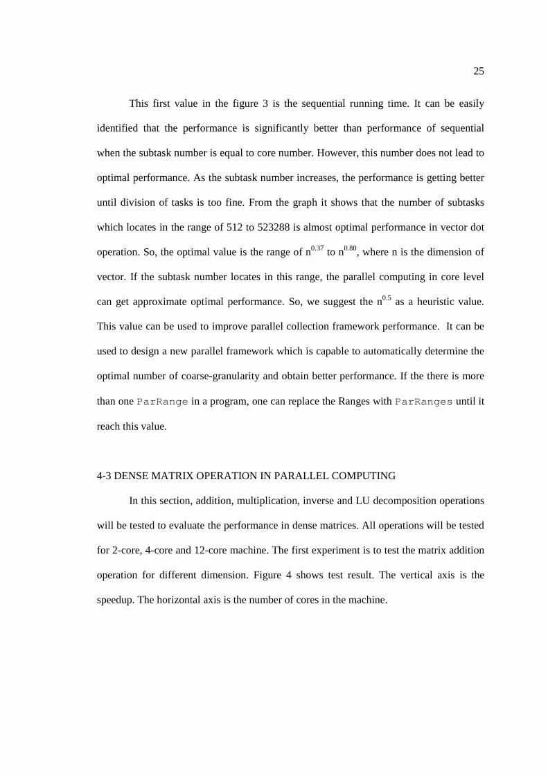
for 2-core, 4-core and 12-core machine. The first experiment is to test the matrix addition

operation for different dimension. Figure 4 shows test result. The vertical axis is the

speedup. The horizontal axis is the number of cores in the machine.

26

Figure 4 dense matrix parallel addition in different dimension

Figure 4 shows that parallel matrix addition is not efficient. It is because the

parallel framework has an overhead cost. If the parallel computing doesn’t save enough

cost, the extra overhead cost will cause it to be less efficient.

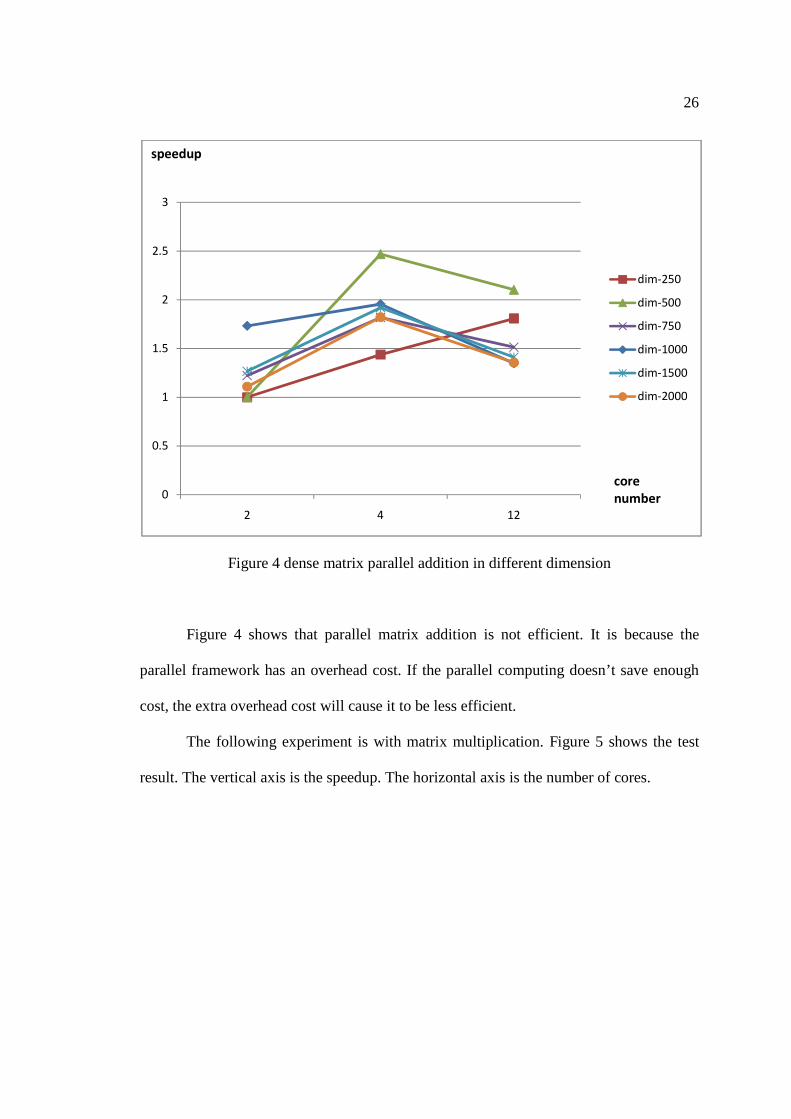
The following experiment is with matrix multiplication. Figure 5 shows the test

result. The vertical axis is the speedup. The horizontal axis is the number of cores.

0

0.5

1

1.5

2

2.5

3

2 4 12

dim-250

dim-500

dim-750

dim-1000

dim-1500

dim-2000

speedup

core

number

27

Figure 5 dense matrix parallel multiplications in different dimension

The result shows that a significant improvement when a parallel framework is

applied. The performance is growing as the number of cores increase. Although

ParRange performs well, there are some other approaches that can be applied that

cause an improvement in matrix multiplication. The first method is to transpose the

second matrix when we do the matrix multiplication. Matrix multiplication causes a

caching problem when performing the matrix multiply as a row is not contiguous in

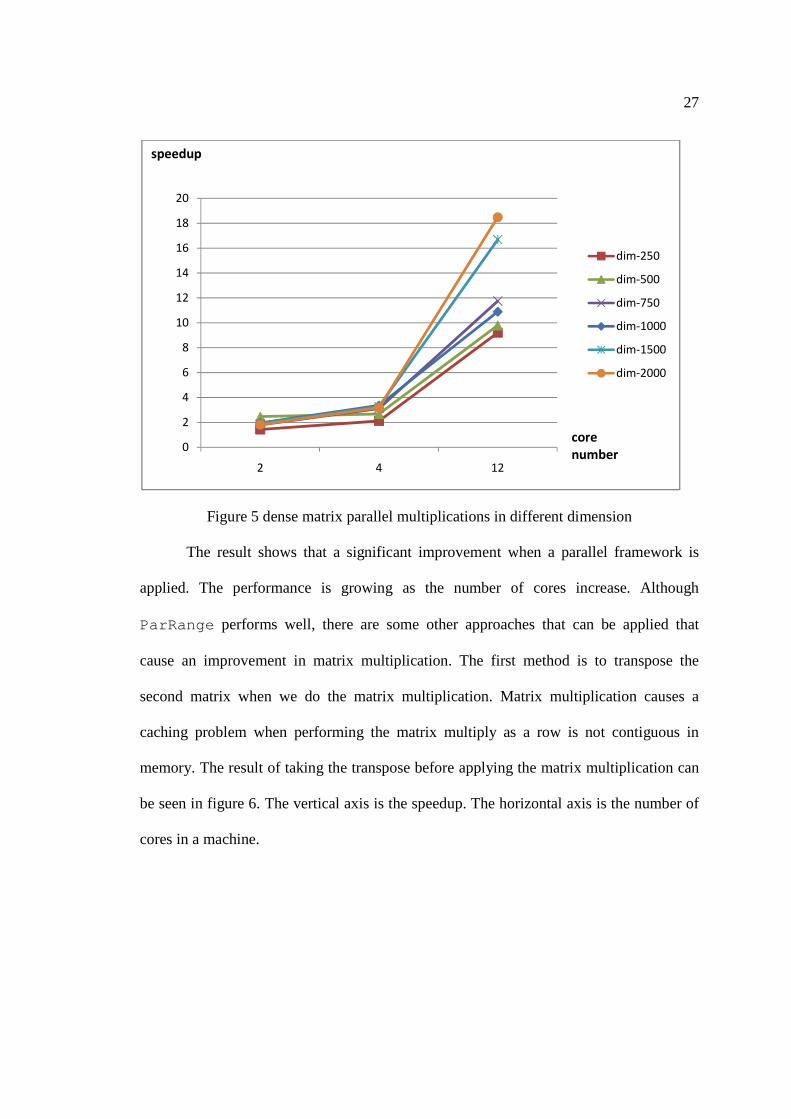
memory. The result of taking the transpose before applying the matrix multiplication can

be seen in figure 6. The vertical axis is the speedup. The horizontal axis is the number of

cores in a machine.

0

2

4

6

8

10

12

14

16

18

20

2 4 12

dim-250

dim-500

dim-750

dim-1000

dim-1500

dim-2000

speedup

core

number

28

Figure 6 dense matrix parallel transpose & multiplication in different dimension

The running time in a 4-core machine is 10 folds improvement. The figure 7

shows the running time required in different dimension. The vertical axis is the time

needed for computation. The horizontal axis is the dimension of matrix.

0

2

4

6

8

10

12

2 4 12

dim-250

dim-500

dim-750

dim-1000

dim-1500

dim-2000

speedup

core

number

29

Figure 7 dense matrix parallel multiplication running time in different dimension

In 1969, Volker Strassen developed an algorithm for performing matrix

multiplication faster than the cubic time. The general idea is to decompose a big square

matrix to 4 smaller sub-matrices. It needs 7 matrix multiplication in these sub matrices

and several addition and minus matrix operations. This will be an ideal test to see the

parallel MatrixD performance when they are applied into other program. The source

code is shown on the Appendix. In this experiment, Strassen fast matrix multiplication

will have only up 6% improvement as the matrix dimension is large. Figure 8 shows

parallel computing speedup result. The vertical axis is the speedup. The horizontal axis is

the dimension of matrix.

1

10

100

1000

10000

100000

1000000

0 500 1000 1500 2000 2500

2-core-seq

4-core-seq

12-core-seq

2-core-par

4-core-par

12-core-par

matrix

dimension

running time

milliseconds

30

Figure 8 matrix parallel strassen multiplication speedup in different dimension

The next two dense matrix operation tests are inverse and LU decomposition.

These two operations require the pivot swap process; therefore fewer parts of these

operations can be parallelized when compared to matrix multiplication. Although the

performance is not as good as matrix multiplication, the trend is still similar to matrix

multiplication. Figures 9 and Figure 10 shows parallel computing results for inversion

and LU decomposition, respectively. The vertical axis is the time needed for computation.

The horizontal axis is the number of cores in the machine.

0

0.2

0.4

0.6

0.8

1

1.2

2 4 12

dim-250

dim-500

dim-750

dim-1000

speedup

core

number

31

Figure 9 dense matrix parallel inversions in different dimension

Figure 10 dense matrix parallel LU decomposition in different dimension

0

1

2

3

4

5

6

7

8

2 4 12

dim-250

dim-500

dim-750

dim-1000

dim-1500

dim-2000

speedup

core

number

0

1

2

3

4

5

6

7

2 4 12

dim-250

dim-500

dim-750

dim-1000

dim-1500

dim-1500

speedup

core

number

32

4-4 SPARSE MATRIX OPERATION IN PARALLEL COMPUTING

A dense matrix is represented as two dimension array which data is distributed

uniformly. In this section, SparseMatrixD in ScalaTion library will be used to see the

performance of unevenly distributed data structure in parallel computing. There are two

sparse matrix operation tests. The first test is sparse matrix addition. Figure 11 show the

results. The vertical axis is the speedup. The horizontal axis is the number of core number

in the machine.

Figure 11 sparse parallel matrix addition in different dimension

The result is similar to the dense matrix addition operation because addition takes

a relatively small amount of time to process.

0

0.5

1

1.5

2

2.5

3

3.5

4

4.5

2 4 12

dim-250

dim-500

dim-750

dim-1000

speedup

core

number

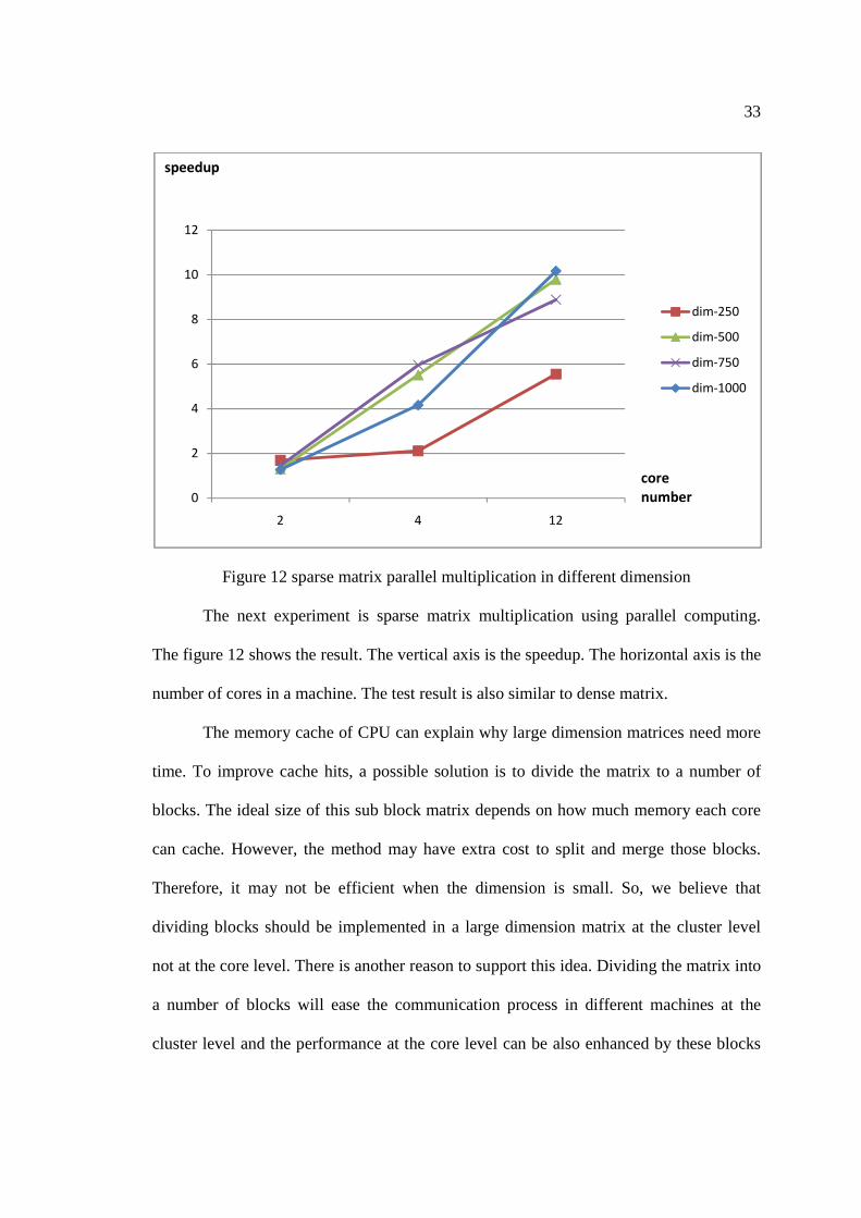
33

Figure 12 sparse matrix parallel multiplication in different dimension

The next experiment is sparse matrix multiplication using parallel computing.

The figure 12 shows the result. The vertical axis is the speedup. The horizontal axis is the

number of cores in a machine. The test result is also similar to dense matrix.

The memory cache of CPU can explain why large dimension matrices need more

time. To improve cache hits, a possible solution is to divide the matrix to a number of

blocks. The ideal size of this sub block matrix depends on how much memory each core

can cache. However, the method may have extra cost to split and merge those blocks.

Therefore, it may not be efficient when the dimension is small. So, we believe that

dividing blocks should be implemented in a large dimension matrix at the cluster level

not at the core level. There is another reason to support this idea. Dividing the matrix into

a number of blocks will ease the communication process in different machines at the

cluster level and the performance at the core level can be also enhanced by these blocks

0

2

4

6

8

10

12

2 4 12

dim-250

dim-500

dim-750

dim-1000

speedup

core

number

34

since every block is still an independent matrix. In next section we will present an

efficient distributed solution for processing the dense and sparse matrix multiplication

operations.

4-5 DISTRIBUTED MATRIX MULTIPLICATION IN PARALLEL COMPUTING

In the previous section, the result of dense parallel matrix and sparse parallel

matrix multiplication shows that the performance is enhanced efficiently by the parallel

framework, ParRange. In this section, an efficient matrix multiplication cluster

program is introduced. There are 4 machines in this cluster and each machine has at least

a 4-cores and 4-gigabyte memory. Although some machine may have more memory, we

will still limit the usage of memory to 4 Gigabytes. There are two goals in this

experiment. The first one is to expand the limitation of the dimension of dense matrix.

The second one is to enhance the performance and be scalable as the dimension of the

matrix increases. To expand the limitation of dense matrix dimension, a good plan to

manage the memory in each machine is required. In order to overcome this limitation, the

big dense matrix should be divided into 4 parts and each machine should hold one part

data of this big dense matrix. In order to reduce the message passing time, each machine

should pass a minimum amount of data during matrix multiplication. In the real world,

there are some applications which require in-place matrix multiplication, such as Markov

Clustering algorithm. So, we will simplify matrix multiplication as in-place matrix

multiplication in this cluster program. In order to enhance the performance at the core

level and ease the communication among machines, the large dense matrix should be

divided into blocks. The size of each block is very important. If too small block size is

35

chosen, it may lead to increased message passing throughout the whole process and waste

too much time on latency. If a too large block size is chosen, the cache memory issue

becomes a factor to slow down the performance. Because of these two reasons, it is hard

to have a general solution that can be applied to every case. The user has to decide the

block size basing on their environment. There are one master machine and 4 worker

machine in this system. The master machine is responsible for synchronizing process and

sending data to each worker machine. The worker machine is responsible for storing and

doing computation during the whole process. Once the block size is determined, the

master machine will start to partition the big dense matrix to several parts. In this

experiment, we will use the column-oriented block partition which means that the large

dense matrix will divide into 4 major column blocks and send to each worker machine to

store in their memory. When a worker machine received all data, it will send a signal to

master machine to notify it has finished. The master machine will wait until all worker

machines receive their data. Then, the master machine will notify every worker machine

to start the matrix multiplication process. Every machine will start to request and receive

the data from other worker machines to compute the first row of block and repeat the

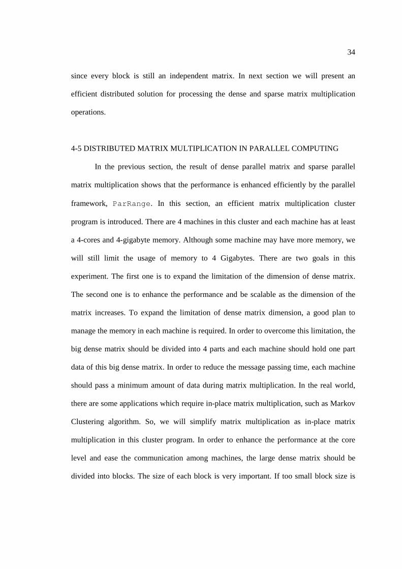
same process on the following rows until all the computation is completed. The figure 14

demonstrates the whole process of the data passing.

36

Figure 13 process of the data passing in cluster level

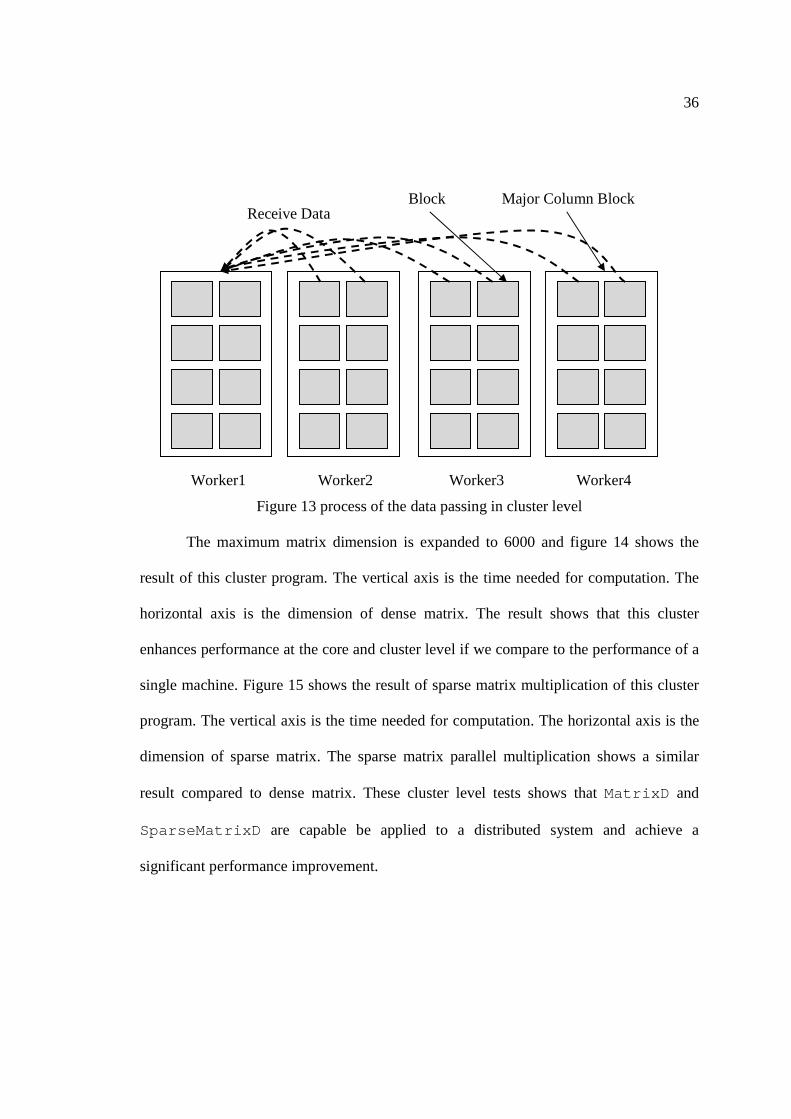
The maximum matrix dimension is expanded to 6000 and figure 14 shows the

result of this cluster program. The vertical axis is the time needed for computation. The

horizontal axis is the dimension of dense matrix. The result shows that this cluster

enhances performance at the core and cluster level if we compare to the performance of a

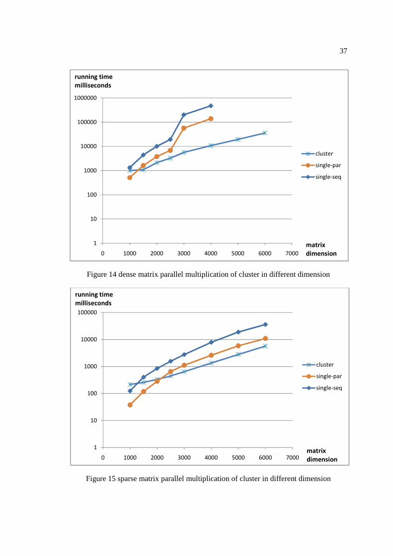
single machine. Figure 15 shows the result of sparse matrix multiplication of this cluster

program. The vertical axis is the time needed for computation. The horizontal axis is the

dimension of sparse matrix. The sparse matrix parallel multiplication shows a similar

result compared to dense matrix. These cluster level tests shows that MatrixD and

SparseMatrixD are capable be applied to a distributed system and achieve a

significant performance improvement.

Major Column Block Block

Worker1 Worker2 Worker3 Worker4

Receive Data

37

Figure 14 dense matrix parallel multiplication of cluster in different dimension

Figure 15 sparse matrix parallel multiplication of cluster in different dimension

1

10

100

1000

10000

100000

1000000

0 1000 2000 3000 4000 5000 6000 7000

cluster

single-par

single-seq

matrix

dimension

running time

milliseconds

1

10

100

1000

10000

100000

0 1000 2000 3000 4000 5000 6000 7000

cluster

single-par

single-seq

matrix

dimension

running time

milliseconds

38

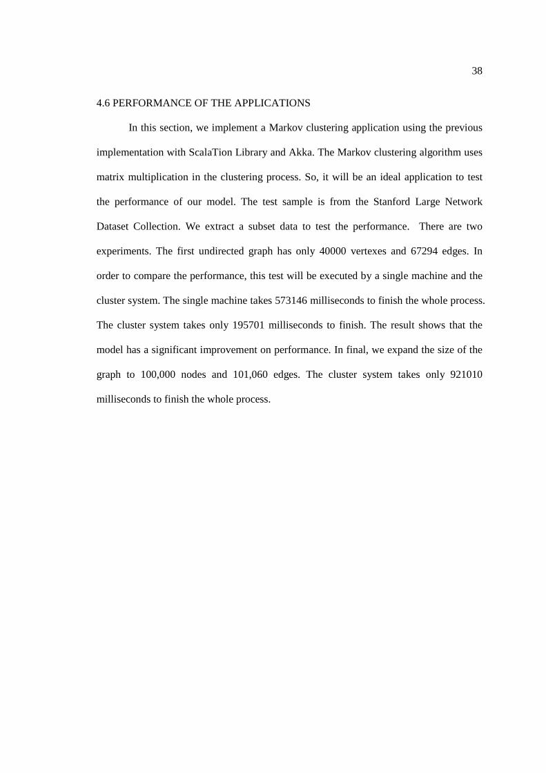
4.6 PERFORMANCE OF THE APPLICATIONS

In this section, we implement a Markov clustering application using the previous

implementation with ScalaTion Library and Akka. The Markov clustering algorithm uses

matrix multiplication in the clustering process. So, it will be an ideal application to test

the performance of our model. The test sample is from the Stanford Large Network

Dataset Collection. We extract a subset data to test the performance. There are two

experiments. The first undirected graph has only 40000 vertexes and 67294 edges. In

order to compare the performance, this test will be executed by a single machine and the

cluster system. The single machine takes 573146 milliseconds to finish the whole process.

The cluster system takes only 195701 milliseconds to finish. The result shows that the

model has a significant improvement on performance. In final, we expand the size of the

graph to 100,000 nodes and 101,060 edges. The cluster system takes only 921010

milliseconds to finish the whole process.

39

Table 3 dense matrix addition running time in different dimension and core number

dimension 2-core 4-core 12-core

Sequential parallel sequential parallel sequential parallel

250 1 4 1 4 1 1 500 5 5 2 4 3 2 750 11 9 9 6 8 3

1000 26 15 10 8 16 5 1500 38 30 20 11 45 23 2000 71 64 30 21 64 22

Time: milliseconds

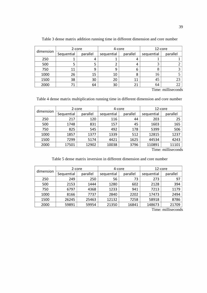
Table 4 dense matrix multiplication running time in different dimension and core number

dimension 2-core 4-core 12-core

Sequential parallel sequential parallel sequential parallel

250 217 120 116 44 203 25

500 1748 831 157 45 1603 165

750 825 545 492 178 5399 506

1000 1857 1377 1339 512 12815 1237

1500 7299 5174 4421 1625 44534 4243

2000 17501 12902 10038 3796 110891 11101

Time: milliseconds

Table 5 dense matrix inversion in different dimension and core number

dimension 2-core 4-core 12-core

Sequential parallel sequential parallel sequential parallel

250 249 250 56 73 273 97

500 2153 1444 1280 602 2128 394

750 6797 4368 1233 941 7213 1179

1000 8166 7737 2840 2202 17473 2494

1500 26245 25463 12132 7258 58918 8786

2000 59891 59954 21350 16841 148673 21709

Time: milliseconds

40

Table 6 dense matrix LU decomposition in different dimension and core number

dimension 2-core 4-core 12-core

Sequential parallel sequential parallel sequential parallel

250 97 99 18 38 103 67

500 773 487 476 369 806 299

750 2481 1672 354 351 2719 726

1000 1836 1713 901 690 6403 1528

1500 6436 6216 3189 1906 21841 4468

2000 15290 14821 7641 4481 69476 10907

Time: milliseconds

Table 7 sparse matrix addition in different dimension and core number

dimension 2-core 4-core 12-core

Sequential parallel sequential parallel sequential parallel

250 13 4 5 2 6 5

500 12 8 9 2 27 18

750 24 16 12 5 58 37

1000 57 25 26 11 110 76

1500 102 146 45 48 202 185

Time: milliseconds

Table 8 sparse matrix multiplication in different dimension and core number

dimension 2-core 4-core 12-core

Sequential parallel sequential parallel sequential parallel

250 81 48 52 21 111 20

500 700 536 434 193 2332 238

750 2718 1873 1582 608 1777 200

1000 6580 5180 3944 1819 4890 481

1500 106019 96471 49379 40850 36469 1957

Time: milliseconds

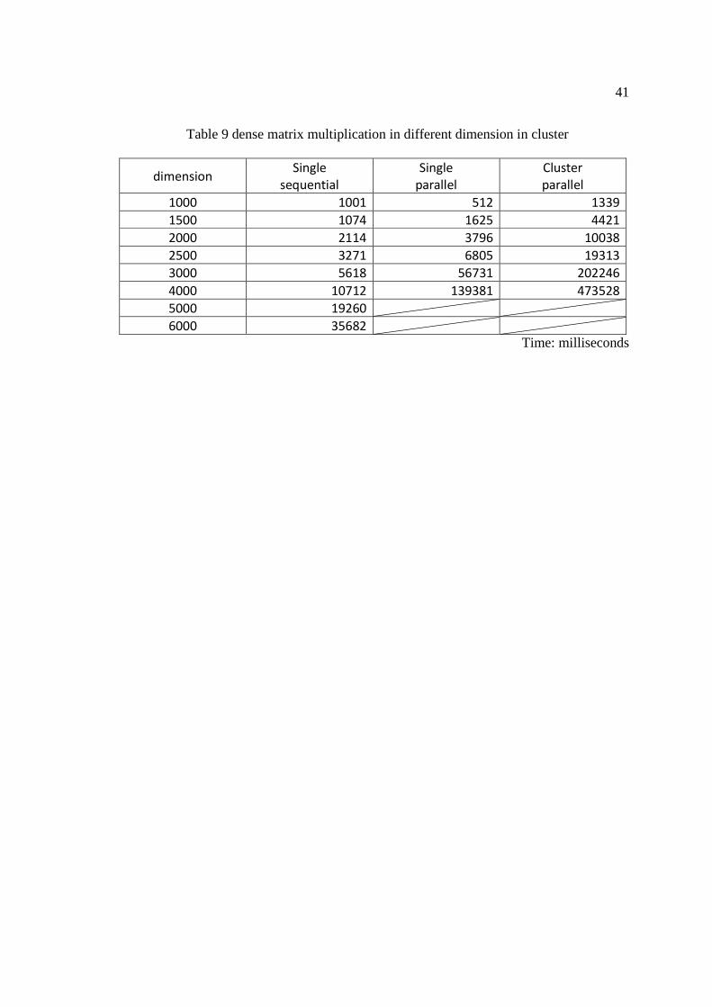
41

Table 9 dense matrix multiplication in different dimension in cluster

dimension Single

sequential

Single

parallel

Cluster

parallel

1000 1001 512 1339 1500 1074 1625 4421 2000 2114 3796 10038 2500 3271 6805 19313 3000 5618 56731 202246 4000 10712 139381 473528 5000 19260

6000 35682

Time: milliseconds

42

CHAPTER 5

COCULDSIONS AND FUTURE WORK

In this report we implemented and tested two parallel matrix structures in the

ScalaTion library. These two structures have shown significantly improved performance

at the core level. At the cluster level, we also present a message passing model built with

Akka which also achieves an improved speedup. These two test results show that by

using a high-level language and a simple message passing model, one can develop

efficient parallel implementations. We also study and test the parallel collection

framework of Scala. We suggest a granularity value which can be used to improve the

performance of the parallel collection framework of Scala. This suggested granularity

value given in chapter 4 shows improvement on programs which suffers from the

granularity issue. We also present a new SortedLinkedHashMap data structure which can

be used for sparse matrices to enhance performance for several operations, not just matrix

multiplication. Moreover, utilizing Scala’s parallel collection framework, our

implementation of sparse matrices can achieve good performance without writing any

complex code.

In the future, we wish to introduce convenient customized parallel control

structures to relieve the burden on programmers who wish to build efficient parallel

programs. With the aid of these control structures, a programmer should be able to easily

convert their sequential programs into parallel programs, thereby improving their

performance.

43

Although many of classes in the parallel linear algebra (linalgebra_par) package

have been made parallel, there are still some classes that are only sequential and need to

be made parallel. Functional programming in general, and Scala particular, may results in

greater memory requirements. Therefore, efforts are needed to streamline the use of

memory as much as possible. The preliminary evaluation given in this report needed to

be replaced with a more comprehensive evaluation on the 12 machines 144-core

computing cluster. This evaluation should also compare the performance with other

related package as well as solution utilizing Map/Reduce or Hadoop solutions. Finally,

we plan to develop further applications for the parallel linear algebra (linalgebra_par)

package in the domain of big data analytics.

44

REFERENCES

[1] Behrooz Parhami, Introduction to Parallel Processing: Algorithms and Architectures

[2] BGI, http://www.bgisequence.com/eu/

[3] Scala, http://www.scala-lang.org/

[4] Akka, http://akka.io/

[5] ScalaTion, http://www.cs.uga.edu/~jam/scalation/README.html

[6] Kevin Hammond, "Why Parallel Functional Programming Matters: Panel Statement"

School of Computer Science, University of St. Andrews, UK

[7] A next-generation parallel file system for Linux cluster: Latham, R.; Miller, N.; Ross,

R.; Carns, P.; Mathematics and Computer Science; Clemson Univ.

[8] Aleksandar Prokopec, Tiark Rompf, Phil Bagwell, Martin Odersky, "A Generic

Parallel Collection Framework", EPFL

[9] Doug Lea, A Java Fork/Join Framework, 2000.

[10] Petra Berenbrink, Tom Friedetzky, and Leslie Ann Goldberg : “The Natural Work-

Stealing Algorithm is Stable”,

[11] Guojing Cong, Sreedhar Kodali, Sriram Krishnamoorthy, Doug Lea, Vijay Saraswat,

Tong Wen, Solving Large, Irregular Graph Problems Using Adaptive Work Stealing,

Proceedings of the 2008 37th International Conference on Parallel Processing, 2008.

[12] Robert A. van de Geijn The University of Texas at Austin : “A Systematic Approach

to Matrix Computations”

[13] B Randell - ACM SIGPLAN Notices: “System Structure for Software Fault

Tolerance:”

45

[14] Jeffrey Dean, Sanjay Ghemawat, “MapReduce: Simplified Data Processing on Large

Clusters”, Google, Inc.

[15] Apache Hadoop, http://hadoop.apache.org/

[16] Sangwon Seo, Edward J. Yoon, Jaehong Kim, Seongwook Jin, Jin-Soo Kim, Seungryoul

Maeng, “HAMA: An Efficient Matrix Computation with the MapReduce

Framework”, KAIST Department of Computer Science, July 06, 2010

[17] "PSBLAS" http://www.ce.uniroma2.it/psblas

[18] Salvatore filippone, IBM Italia and Michele ColaJanni, Università di Modena e

Reggio Emilia (2000). PSBLAS : A Library for Parallel Linear Algebra Computation

on Sparse Matrices

46

APPENDIX

Source code of SparseMatrixD :

def * (b: SparseMatrixD): SparseMatrixD =

{

val c = new SparseMatrixD (dim1, b.dim2)

val bt = b.t

for (i <- c.range1) {

var ea: (Int, Double) = null // element in row of this matrix

var eb: (Int, Double) = null // element in row of bt matrix

for (j <- c.range2) {

val ita = v(i).iterator

val itb = bt.v(j).iterator

var cont = false

var itaNext = true // more elements in row?

var itbNext = true // more elements in row?

var sum = 0.

if (ita.hasNext && itb.hasNext) cont = true

while (cont) {

if (itaNext) ea = ita.next () // (j, v) for this

if (itbNext) eb = itb.next () // (j, v) for bt

if (ea._1 == eb._1) { // matching indexes

sum += ea._2 * eb._2

itaNext = true; itbNext = true

} else if (ea._1 > eb._1) {

itaNext = false; itbNext = true

} else if (ea._1 < eb._1) {

itaNext = true; itbNext = false

47

} // if

if (itaNext && !ita.hasNext) cont = false

if (itbNext && !itb.hasNext) cont = false

} // while

if (sum != 0.) c(i, j) = sum // assign if non-zero

} // for

} // for

c

} // *

48

Source code of Strassen Fast Matrix Multiplication

def strassenMult (b: MatrixD): MatrixD =

{

val c = new MatrixD (dim1, dim1) // allocate result matrix

var d = dim1 / 2 // half dim1

if (d + d < dim1) d += 1 // if not even, increment by 1

val evenDim = d + d

// decompose to blocks (use vslice method if available)

val a11 = slice (0, d, 0, d)

val a12 = slice (0, d, d, evenDim)

val a21 = slice (d, evenDim, 0, d)

val a22 = slice (d, evenDim, d, evenDim)

val b11 = b.slice (0, d, 0, d)

val b12 = b.slice (0, d, d, evenDim)

val b21 = b.slice (d, evenDim, 0, d)

val b22 = b.slice (d, evenDim, d, evenDim)

// compute intermediate sub-matrices

val p1 = (a11 + a22) * (b11 + b22)

val p2 = (a21 + a22) * b11

val p3 = a11 * (b12 - b22)

val p4 = a22 * (b21 - b11)

val p5 = (a11 + a12) * b22

val p6 = (a21 - a11) * (b11 + b12)

val p7 = (a12 - a22) * (b21 + b22)

for (i <- c.range1; j <- c.range2) {

c.v(i)(j) =

if (i < d && j < d) {

p1.v(i)(j) + p4.v(i)(j)- p5.v(i)(j) + p7.v(i)(j)

49

} else if (i < d) {

p3.v(i)(j-d) + p5.v(i)(j-d)

} else if (i >= d && j < d) {

p2.v(i-d)(j) + p4.v(i-d)(j)

} else {

p1.v(i-d)(j-d) - p2.v(i-d)(j-d) +

p3.v(i-d)(j-d) + p6.v(i-d)(j-d)

}

} // for

c // return result matrix

} // strassenMult